The Nonlinear Limit-PointLimit-Circle Problem for Higher Order Equations

合集下载

非线性方程和非线性方程组的迭代解法

则称序列（Ｘ。）至少Ｐ阶收敛．当ｐ＝ｌ，０＜Ｃ＜１时，称序列（ｘ“）至少线性收
敛：ｐ＝２，ｃ＞０称序列至少平方收敛；若ｋ≥ｋ．，时，有Ｘｋ＝ｘ４成立，或
ｌｉｍ堕：。二型＝０
“‘｜｜Ｘ“一Ｘ＋旷则称事列（Ｘ）为超ｐ阶收敛
定义４［１３假定迭代序列（ｘ。｝收敛于ｘ＋，量
！抽婪∑梨，当ｘｔ≠ｘ·对ｋ≥ｋ。。
（１）公式的建立
设ｘ＋是方程ｆ（ｘ）＝ｏ的解，ｆ（ｘ）在ｘ＋的某邻域Ａ＝｛ｘｊｘ—ｘ４≤６｝存在
二阶导数，且ＶＸ∈Ａ，ｆ’（Ｘ）≠０，设ｘ。∈△为ｆ的近似值，将ｆ（ｘ）在Ｘ。处展为一次Ｔａｙｌｏｒ多项式ｆ（Ｘ）＝ｆ（ｘｋ）＋ｆ７（ｘ。）（ｘ—ｘ。），记ｐ（Ｘ）＝ｆ（ｘ．）十ｆ’（Ｘ：）（Ｘ—Ｘ．），显然Ｐ（Ｘ）≈ｆ（ｘ）．令Ｐ（ｘ）＝Ｏ，解得
应用这个方法求解了非线性偏微分方程ｕ．＋“萎生等｝＜如Ｖ＞。Ｑ，ｓ（ｕ）＝。，其中
Ｑ“ｕ）２与竿导，万—ｉｉＦ数值计算中得到的非线性方程组，并通过迭代公
式（４－３）与Ｎｅｗｔｏｎ法的数值实验结果的比较，晚明了在相同精度要求卜Ｉ求解这个问题时，ｆ＝｝｝式ｆ４—３）优于＼ｅｎｔＯｔｌ法的几个方面．
第一章解非线性方程的常用迭代格式
在第三章写出了这几个迭代公式的相应算法设计，并将这些格式的数值实验结果与Ｎｅｗｔｏｎ法、弦截法、Ｍｕｌｌｅｒ法的数值实验结果进行了比较，说明了这几个迭代格式的有效性．
在第四章中将预测式迭代法推广到了求解非线性方程组，分析了它的收敛性、收敛阶，给出了其算法设计并进行了数值实验证明了方法的有效性．特别地，
兰州大学硕士学位论文非线性方程和非线性方程组的迭代解法及姓名：尚秀丽申请学位级别：硕士专业：计算数学指导教师：周宇斌
20041101

20140621文献阅读示例

M. Ishitobi and M. Nishi are with the Department of Mechanical Systems Engineering, Kumamoto University, Kumamoto 860-8555, Japan mishi@kumamoto-u.ac.jp
approximate model may fail to stabilize the exact discretetime model [2]. Recently, Yuz and Goodwin have proposed an accurate sampled-data model [3]. The resulting model includes extra zero dynamics which are called sampling zero dynamics. It has been shown explicitly that they have no counterpart in the underlying continuous-time system and are the same as those for the linear case [4], although an implicit characterization has been given in [5]. It is worth noting here that Yuz and Goodwin’s model has a mode corresponding to the sampling zero dynamics just on the unit circle when the relative degree of a continuous-time nonlinear system is two. This paper shows that a more accurate sampled-data model is required for a controlled Van der Pol system with the relative degree two. The reason is that the closed-loop system becomes unstable when a controller design method based on cancellation of the zero dynamics is applied, and the phenomenon seems related to the instability of the sampling zero dynamics of the more accurate sampled-data model. Further, this paper derives a more accurate model than that of Yuz and Goodwin for continuous-time nonlinear systems with the relative degree two, and shows a condition which assures the stability of the sampling zero dynamics of the obtained model. For linear systems, the properties of the sampling zeros corresponding to the sampling zero dynamics for nonlinear systems are discussed in many papers [4], [6]-[11]. II. SYSTEM DESCRIPTION AND PREVIOUS RESULTS Consider a class of the following single-input singleoutput nth-order nonlinear system ⎧ ˙ = f (x) + g (x)u ⎨ x (1) ⎩ y = h(x) where x is the state evolving on an open subset M ⊂ Rn , and where the vector ﬁelds f (·) and g (·), and the output function h(x) are analytic on M. First, the following assumptions are introduced. Assumption 1: The unique equilibrium point lies on the origin. Assumption 2: The continuous-time nonlinear system (1) has the uniform relative degree r(≤ n) and is minimum phase in the open subset M, where the state x evolves. Then, the system can be expressed in its so-called normal

台湾国立交通大学

台湾国⽴交通⼤学数学视频数学视频Calculus I 台湾国⽴交通⼤学 Michael Fuchs⽼師 36集（点击进⼊我的淘宝店）Calculus II 台湾国⽴交通⼤学 Michael Fuchs⽼師 29集（点击进⼊我的淘宝店）Chapter1　Functions and Model1-5　Exponential Functions1-6　Inverse Functions and LogarithmsChapter2　Limits and Derivatives2-2　The Limit of a Function2-4　The Precise Definition of a Limit2-3　Calculating Limits Using the Limit Laws2-6　Limits at Infinity; Horizontal Asymptotes2-5　Continuity2-8　Derivatives2-9　The Derivative as a FunctionChapter3　Differentiation Rules3-1　Derivatives of Polynomials and Exponential Functions3-2　The Product and Quotient Rules3-4　Derivatives of Trigonometric Functions3-5　The Chain Rule3-6 Implicit Differentiation3-8 Derivatives of Logarithmic Functions3-10　Related Rates3-7 Higher Derivatives3-11　Linear Approximations and DifferentialsChapter4　Applications of Differation4-1　Maximum and Minimum Values4-2　The Mean Value Theorem4-3 How Derivatives Affect the Shape of a Graph4-4 Indeterminate Forms a nd L’Hospital’s Rule4-7　Optimization Problems4-5　Summary of Curve Sketching4-10　AntiderivativesChapter5　Integrals5-1　Areas and Distances5-2　The Definite Integral5-3　The Fundamental Theorem of Calculus5-4　Indefinite Integrals and the Total Change Theorem5-5　The Substitution Rule5-6　The Logarithm Defined as an IntegralChapter6　Applications of Integration6-1　Areas between Curves6-2　Volumes6-3　Volumes be Cylindrical ShellsChapter7　Techniques of Integration7-1　Integration by Parts7-2　Trigonometric Integrals7-3　Trigonometric Substitution7-4　Integration of Rational Functions by Partial Fractions7-8　Improper Integrals7-7　Approximate IntegrationChapter8　Further Applications of Integration8-1　Arc Length8-2　Area of a Surface of RevolutionChapter10　Parametric Equations and Polar Coordinates10-1　Curves Defined by Parametric Equations10-2　Calculus with Parametric Curves10-3　Polar Coordinates10-4　Areas and Lengths in Polar Coordinates微积分(⼀) 台湾国⽴交通⼤学莊重⽼師　24集（点击进⼊我的淘宝店）微积分(⼆)台湾国⽴交通⼤学莊重⽼師 24集（点击进⼊我的淘宝店）課程章節第⼀章Functions and Model第⼆章Limits and derivatives第三章Differentiation Rules第四章The Properties of Gases第五章Integrals第六章Applications of Integration第七章Techniques of Integration第⼋章Further Applications of Integration第⼗章Parametric Equations and Polar Coordinates第⼗⼀章Infinite Sequences and Series第⼗⼆章Vectors and the Geometry of Space第⼗三章Vector Functions第⼗四章Partial Derivatives第⼗五章Multiple Integrals⾼等微积分(⼀)台湾国⽴交通⼤学⽩啟光⽼師　29集（点击进⼊我的淘宝店）⾼等微积分(⼆) 台湾国⽴交通⼤学　⽩啟光⽼師　27集（点击进⼊我的淘宝店）第⼀章The Real and Complex Number SystemsFields Axioms, Order Axioms　Completeness Axioms第⼆章Basic TopologyCardinality of SetsMetric SpacesCompact SetsConnected Sets第三章Numerical Sequences and SeriesConvergent SequencesCauchy SequencesUpper and Lower LimitsSeries of Nonnegative TermsThe Root and Ratio TestAbsolute Convergence, Rearrangements第四章ContinuityLimits of Functions and Continuous FunctionsContinuity and CompactnessContinuity and Connectednessdiscontinuities, Infinite Limits and Limits at Infinity第五章Differentiation　The Derivative of a Real Function, Mean Value TheoremL’Hopital’s RuleTaylor’s TheoremDifferentiation of Vector-valued Functions第六章The Riemann-Stieltjes Integral　Definition and Existence of the IntegralProperties of the IntegralIntegration and DifferentiationIntegration and Differentiation第六章The Riemann-Stieltjes IntegralIntegration and Differentiation第七章Sequence and Series of FunctionsSequence and Series of Functions --- the Main ProblemUniform Convergence and ContinuityUniform Convergence and IntegrationUniform Convergence and DifferentiationEquicontinuous Family of FunctionsThe Stone-Weierstrass Theorem第⼋章Some Special FunctionsPower seriesSome Special FunctionsFourier SeriesThe Gamma Function第九章Functions of several variablesFunction of Several VariablesFunction of Several Variables：DifferentiationFunction of Several Variables：DifferentiationThe Inverse Function TheoremThe Implicit Function TheoremThe Rank TheoremDeterminantsDifferentiation of Integrals偏微分⽅程(⼀) 台湾国⽴交通⼤学林琦焜⽼师 3.8GB （点击进⼊我的淘宝店）偏微分⽅程(⼆) 台湾国⽴交通⼤学林琦焜⽼师 3.4GB （点击进⼊我的淘宝店）内容纲要第⼀章 The Single First-Order Equation1-1 Introduction Partial differential equations occur throughout mathematics. In this part we will give some examples1-2 Examples1-3 Analytic Solution and Approximation methods in a simple example 1-st order linear example1-4 Quasilinear Equation The concept of characteristic1-5 The Cauchy Problem for the Quasilinear-linear Equations1-6 Examples Solved problems1-7 The general first-order equation for a function of two variables characteristic curves, envelope1-8 The Cauchy Problem characteristic curves, envelope1-9 Solutions generated as envelopes第⼆章Second-Order Equations: Hyperbolic Equations for Functions of Two Independent Variables2-1 Characteristics for Linear and Quasilinear Second-Order Equations Characteristic2-2 Propagation of Singularity Characteristic curve and singularity2-3 The Linear Second-Order Equation classification of 2nd order equation2-4 The One-Dimensional Wave Equation dAlembert formula, dimond law, Fourier series2-5 System of First-Order Equations Canonical form, Characteristic polynominal2-6 A Quasi-linear System and Simple Waves Concept of simple wave第三章 Characteristic Manifolds and Cauchy Problem3-1 Natation of Laurent Schwartz Multi-index notation3-2 The Cauchy Problem Characteristic matrix, characteristic form3-3 Real Analytic Functions and the Cauchy-Kowalevski Theorem Local existence of solutions of the non-characteristic 3-4 The Lagrange-Green Identity Gauss divergence theorem3-5 The Uniqueness Theorem of Ho ren Uniqueness of analytic partial differential equations3-6 Distribution Solutions Introdution of Laurent Schwartzs theory of distribution (generalized function)第四章 The Laplace Equation4-1 Greens Identity, Fundamental Solutions, and Poissons Equation Dirichlet problem, Neumann problem, spherical symmetry, mean value theorem, Poisson formula4-2 The Maximal Principle harmonic and subharmonic functions4-3 The Dirichlet Problem, Greens Function, and Poisson Formula Symmetric point, Poisson kernel4-4 Perrons method Existence proof of the Dirichlet problem4-5 Solution of the Dirichlet Problem by Hilbert-Space Methods Functional analysis, Riesz representation theorem, Dirichlet integra第五章 Hyperbolic Equations in Higher Dimensions5-1 The Wave Equation in n-Dimensional Space(1) The method of sphereical means(2) Hadmards method of descent(3) Duhamels principle and the general Cauchy problem(4) mixed problem5-2 Higher-Order Hyperbolic Equations with Constant Coefficients(1) Standard form of the initial-value problem(2) solution by Fourier transform,(3) solution of a mixed problem by Fourier transform5-3 Symmetric Hyperbolic System(1) The basic energy inequality(2)Finite difference method(3) Schauder method第六章 Higher-Order Elliptic Equations with Constant Coefficients6-1 The Fundamental Solution for Odd n Travelling wave6-2 The Dirichlet Problem Lax-Milgram theorem, Garding inequality6-3 Sobolev Space Weak solution and Hibert space第七章 Parabolic Equations7-1 The Heat Equation Self-Similarity, Heat kernel, maximum principle7-2 The Initial-Value Problem for General Second-Order Parabolic Equations(1) Finite difference and maximum principle(2) Existence of Initial Value Problem第⼋章 H. Lewys Example of a Linear Equation without Solutions8-1 Brief introduction of Functional Analysis Hilbert and Banach spaces, projection theorem, Leray-Schauder theorem8-2 Semigroups of linear operator Generation, representation and spectral properties8-3 Perturbations and Approximations The Trotter theorem8-4 The abstract Cauchy Problem Basic theory8-5 Application to linear partial differential equations Parabolic equation, Wave equation and Schrodinger equation8-6 Applications to nonlinear partial differential equations KdV equation, nonlinear heat equation, nonmlinear Schrodinger equation变分学导论应⽤数学系林琦焜⽼师台湾国⽴交通⼤学 2GB （点击进⼊我的淘宝店）内容纲要第⼀章变分学之历史名题1.1 Bernoulli 最速下降曲线1.2 最⼩表⾯积的迴转体1.3 Plateau问题(最⼩曲⾯)1.4 等周长问题1.5 古典⼒学之问题第⼆章 Euler- Lagrange⽅程2.1 变分之原理2.2 折射定律与最速下降曲线2.3 ⼴义座标2.4 Dirichlet 原理与最⼩曲⾯2.5 Lagrange乘⼦与等周问题2.6 Euler-Lagrage ⽅程之不变量2.7 Sturm-Liouville问题2.8 极值(积分)问题第三章 Hamilton系统3.1 Legendre变换3.2 Hamilton⽅程3.3 座标变换与守恒律3.4 Noether定理3.5 Poisson括号第四章数学物理⽅程4.1 波动⽅程4.2 Laplace与Poisson⽅程4.3 Schrodinger ⽅程4.4 Klein-Gordon ⽅程4.5 KdV ⽅程4.6 流体⼒学⽅程　课程书⽬变分学导论 (Lecture note by Chi-Kun Lin).向量分析台湾国⽴交通⼤学林琦焜 3.3GB （点击进⼊我的淘宝店）向量分析主要是要谈”梯度、散度与旋度”这三个重要观念，⽽对应的则是⽅向导数、散度定理、与Stokes定理因此重⼼就在於如何釐清线积分、曲⾯积分以及他们所代表的物理意义。

高维Euler方程组的强松驰极限

高维Euler方程组的强松驰极限徐志琳; 林春进【期刊名称】《《吉林大学学报（理学版）》》【年(卷),期】2019(057)006【总页数】7页(P1292-1298)【关键词】Euler方程; 松弛; 全局光滑解; 非线性扩散方程【作者】徐志琳; 林春进【作者单位】河海大学理学院南京210098【正文语种】中文【中图分类】O175.270 引言考虑如下高维带松弛项的Euler方程组：(1)其初始条件为ρ(x,0)=ρ0(x), u(x,0)=u0(x).(2)这里: x∈n为空间变量;t>0为时间变量;ε>0为松弛常数;ρ(x,t)∈和u∈n分别表示流体在t时刻、x处的密度和速度;P=P(ρ)表示流体的压强,对于任意的ρ>0,满足P′(ρ)>0.对于Euler方程组整体解的研究目前已有很多成果[1-12]：文献[1]研究了一维Euler方程组在Lagrange坐标下解的大时间行为,并证明了当时间t→∞时,方程组(1)的解收敛于非线性扩散方程的解;文献[5]用流函数的方法证明了等温Euler方程组的解在有界变差的初值条件下收敛于热传导方程的解;文献[6]利用熵变量研究了在初值充分小时,等温Euler方程组的光滑解当ε→0时收敛于热传导方程的解;文献[7]利用熵变量,将文献[6]的结论推广到包含等熵Euler方程组在内的一般Euler方程组上；文献[8]将这类方法推广到一般的松弛极限.但该方法对方程对称子关于变量的依赖关系有较高要求.文献[9]通过引入新的变量,利用Euler方程的等价形式得到了有效的能量估计,从而证明了解的整体存在性；文献[10]在能量估计中利用密度关于时间t的偏导数估计,得到了解的整体存在性；文献[11-12]利用该方法得到了类似的结果.但文献[9-12]中只考虑了带阻尼项的Euler方程解的整体存在性(即ε=1情形),由于缺少关于时间的一致先验估计,因此不能直接用来处理松弛极限.文献[13]讨论了相互作用力下带阻尼的Euler方程的极限模型；文献[14-15]讨论了带阻尼的Euler方程强松弛极限在其他物理模型上的推广.本文借助文献[6-8]的方法和文献[9-10]中能量估计的技巧,建立一般的可压缩Euler方程组的解关于ε的一致先验估计,从而获得光滑解的整体存在性.定理1 设为常数,k∈,且k>[n/2]+1,0<ε≤1,则存在两个正常数C和δ,使得对任意的初值(ρ0,u0)满足方程组(1)关于初值(ρ0,u0)都存在唯一的光滑解(ρε,uε),且满足n)),并对任意的t≥0,有这里C和δ与参数ε和初值(ρ0,u0)均无关.定理2 在定理1的条件下,设(ρε,uε)为方程组(1)关于初值(ρ0,u0)的整体光滑解,记其中τ=εt,若n))为如下非线性扩散方程的解:则对于任意的T>0,X>0且按范数C([0,T];Hk(BX))收敛于R,其中BX={x∈n: |x|<X}.与文献[6-7]相比,定理1的估计更精细,这里包含了∂tρε的估计,利用熵变量的框架,∂tρε的估计不能直接获得.定理2讨论了方程组(1)的强松弛极限,借助于文献[5-6],可以证明密度函数在松弛时间变量下,收敛于非线性扩散方程的解.由定理1中解的一致先验估计,可获得新的时间尺度下变量和借助于LP空间的紧性结论,可获得的渐近行为,从而得到解收敛于多孔渗流方程,故本文省略定理2的证明.本文关于松弛极限的结论与文献[6]一致,但获得解的估计比文献[6]更精细,且本文对松弛模型的研究方法可推广至更一般的物理模型中.若无特殊说明,本文中C均表示一个与ε和初值均无关的正常数,但不同之处可表示不同的值.用α∈n表示多重指标,即α=(α1,α2,…,αn),其中αi∈,i=1,2,…,n,用|α|表示其阶数,即|α|=α1+α2+…+αn.∂α表示关于x的|α|阶偏导数,‖·‖L2,‖·‖L∞,‖·‖Hk分别表示n 上的L2范数、L∞范数和Hk范数.1 一致先验估计先对方程(1)在常状态处做线性化,然后利用标准能量积分获得和uε的L∞(Hk)估计,最后结合方程组(1),消去·(ρεuε),对方程组作进一步的能量估计,获得∂tρε和ρε的L2(Hk-1)估计,从而获得解的整体存在性.令这里是一个常数,则方程组(1)变形为(3)其中(4)由式(3)中的质量守恒方程可得速度变量的散度为(5)对于(V,U)∈C([0,T];Hk(n)),定义能量泛函为若Nε(T)≤δ,则根据Nε(T)的定义以及Sobolev嵌入定理,可知(7)由式(7)式,易见(8)下面进行能量估计,首先证明如下的L∞(Hk)估计:命题1 若扰动方程组(3)的解(V,U)∈C([0,T],Hk(n)),且满足Nε(T)≤δ,则存在常数C,使得对于∀t∈[0,T],有证明: 先将式(3)的第一个方程两边同时关于x求α阶导后与相乘,然后将式(3)中的第二个方程两边同时关于x求α阶导后与相乘,|α|≤k,最后将两式相加,并在n×[0,t]上积分,得下面估计式(10)右端的第一个积分,结合式(5),有其中[,]表示交换子,即[A,B]C=A(BC)-B(AC).对于I1,通过分部积分,有由式(7)知则(13)此外,对式(12)右侧第二项分|α|=0和|α|>0进行讨论：当|α|=0时,有‖V‖L∞≤C‖V‖Hk-1,根据式(7)并结合Hölder不等式及带ε的Young不等式,有当|α|>0时,式(12)右侧第二项的估计更简单,则有把式(13)～(15)代入式(12),可得对于I2,利用交换子的Moser类估计,并参考文献[16],可得由复合函数的Moser类估计,并参考文献[16],有(18)利用式(17),(18)及Sobolev嵌入不等式,有(19)与估计I1和I2的方法类似,对于I3和I4,可估计为(20)根据上述估计技巧,I5和I6的估计较容易,有由估计式(16)～(22),可得下面估计式(10)右端第二个积分,首先利用表达式,可写为与前面的估计类似,利用分部积分,J1可化为对于式(25)右侧第一项,根据式(8)及Hölder不等式易得到估计.对于式(25)右侧第二项,利用式(5),与式(11)中前四项的估计方法类似,有同理,对J2,J3,J4的估计,有(27)由式(26),(27),可得将式(23),(28)代入式(10),当δ充分小时关于|α|≤k求和,即得命题1.下面讨论Vt的估计.命题2 在命题1的条件下,有证明: 首先,对式(3)的第一个方程两边同时关于t求导,对式(3)第二个方程两边同时求散度,再将两式相加,并消去(·U)t,得(29)这里(30)然后,对式(29)两边同时关于x求α阶导,|α|≤k-1,再乘以∂α(εV+Vt),并在n×[0,t]上积分,可得下面估计式(31)右端含有∂αR(V,U)的积分项,利用式(30),把ε∂αR(V,U)∂αV的积分拆成四项：其中：与式(24)中的估计类似,I1,I2和I4可估计为对于I3,利用式(3)的第二个方程,将∂tU用U,V和Q(V,U)表示,I3可分解为与I1,I2和I4的估计同理,利用分部积分与交换子的性质,I3可进一步估计为(35)结合式(32)～(35),可得式(31)右端积分项中的∂αR(V,U)∂αVt的积分的估计式(36)类似,于是将式(36),(37)代入式(31),当δ充分小时,关于|α|≤k-1求和,即得命题2的估计.根据一致先验估计,并由质量守恒可知: Vt(0)=-·[(V0+1)U0],从而可得解的一致先验估计,进而获得解的整体存在性[6,9] .参考文献【相关文献】[1] HSIAO L,LIU Taiping.Convergence to Nonlinear Diffusion Waves for Solutions of a System of Hyperbolic Conservation Laws with Damping [J].Comm Math Phy,1992,143(3): 599-605.[2] NISHIHARA K.Convergence Rates to Nonlinear Diffusion Waves for Solutions of System of Hyperbolic Conservation Laws with Damping [J].J DifferentialEquations,1996,131(2): 171-188.[3] WANG Weike,YANG Tong.Pointwise Estimates and Lp Convergence Rates to Diffusion Waves for p-System with Damping [J].J Differential Equations,2003,187(2): 310-336. [4] ZHAO Huijiang.Convergence to Strong Nonlinear Diffusion Waves for Solutions of p-System with Damping [J].J Differential Equations,2001,174(1): 200-236.[5] JUNCA S,RASCLE M.Strong Relaxation of the Isothermal Euler System to the Heat Equation [J].Z Angew Math Phy,2002,53(2): 239-264.[6] COULOMBEL J F,GOUDON T.The Strong Relaxation Limit of the Multidimensional Isothermal Euler Equations [J].Trans Amer Math Soc,2007,359(2): 637-648.[7] LIN Chunjin,COULOMBEL J F.The Strong Relaxation Limit of the Multidimensional Euler Equations [J].Nonlinear Differential Equations Appl,2013,20(3): 447-461.[8] PENG Yuejun,WASIOLEK V.Uniform Global Existence and Parabolic Limit for Partially Dissipative Hyperbolic Systems [J].J Differential Equations,2016,260(9): 7059-7092.[9] SIDERIS T C,THOMASES B,WANG Dehua.Long Time Behavior of Solutions to the 3D Compressible Euler Equations with Damping [J].Comm Partial DifferentialEquations,2003,28(3/4): 795-816.[10] WANG Weike,YANG Tong.The Pointwise Estimates of Solutions for Euler Equations with Damping in Multi-dimensions [J].J Differential Equations,2001,173(2): 410-450. [11] 熊显萍,朱旭生.带阻尼项的欧拉方程初边值问题的经典解 [J].天津师范大学学报(自然科学版),2014,34(1)：16-19.(XIONG Xianping,ZHU Xusheng.Classical Solution of Initial-Boundary Value Problem for Euler Equations with Damping [J].Journal of Tianjin Normal University (Natural Science Edition),2014,34(1)：16-19.)[12] 熊显萍,黄激姗,王美娜.三维空间中带阻尼项的欧拉方程初边值问题的经典解 [J].西南师范大学学报(自然科学版),2017,42(1)：1-6.(XIONG Xianping,HUANG Jishan,WANG Meina.On Solution of Initial-Boundary Value Problem for 3-Dimensional Euler Equations with Nonlinear Damping [J].Journal of Southwest China Normal University (Natural Science Edition),2017,42(1)：1-6.)[13] CARRILLO J A,CHOI Y P,TSE O.Convergence to Equilibrium in Wasserstein Distance for Damped Euler Equations with Interaction Forces [J].Comm Math Phy,2019,365(1): 329-361.[14] PENG Yuejun,WASIOLEK V.Global Quasi-neutral Limit of Euler-Maxwell Systems with Velocity Dissipation [J].J Math Anal Appl,2017,451(1): 146-174.[15] WASIOLEK V.Uniform Global Existence and Convergence of Euler-Maxwell Systems with Small Parameters [J].Commun Pure Appl Anal,2016,15(6): 2007-2021.[16] MAJDA pressible Fluid Flow and Systems of Conservation Laws in Several Space Variables [M].New York: Springer-Verlag,1984.。

Abaqus仿真分析-CONT-L04-Logic

| © Dassault Systèmes
Undeformed shape
P
Deformed shape (Mises stress contours)
3. Compress tip 2. Contact rigid surface
1. Bend beam
Challenging for Newton method!
L4.1
Lesson 4: Contact Logic and Diagnostics Tools
The following topics are covered in this lesson.
Lesson content: Contact Logic and Diagnostics Tools Workshop 3: Bolted Flange Analysis (IA) Workshop 3: Bolted Flange Analysis (KW)
| © Dassault Systèmes
L4.11
The Contact Algorithm (4/5)
4 Has convergence been achieved? By default, Abaqus quantifies the contact incompatibilities associated with SDIs. These incompatibilities must be sufficiently small to achieve convergence with respect to the contact state. Also have to ensure that the force residuals and solution corrections are sufficiently small to achieve equilibrium. If the contact state and equilibrium conditions satisfy their respective convergence criteria, the increment is complete.

Bifurcation+Theory

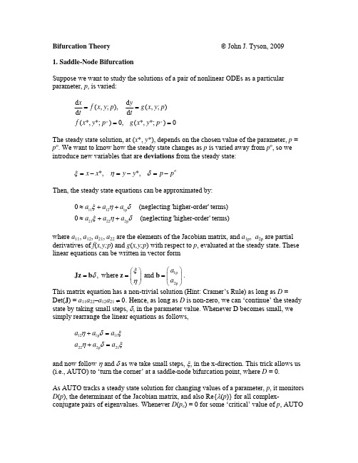
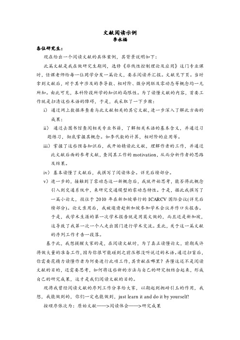
Bifurcation Theory © John J. Tyson, 20091. Saddle-Node BifurcationSuppose we want to study the solutions of a pair of nonlinear ODEs as a particular parameter, p , is varied:d d (,;), (,;)d d (*,*;)0, (*,*;)0o o x y f x y p g x y p t tf x y pg x y p ====The steady state solution, at (x *, y *), depends on the chosen value of the parameter, p = p o . We want to know how the steady state changes as p is varied away from p o , so we introduce new variables that are deviations from the steady state:*, *, o x x y y p p ξηδ=−=−=−Then, the steady state equations can be approximated by:11121p 21222p 0 (neglecting 'higher-order' terms)0 (neglecting 'higher-order' terms)a a a a a a ξηδξηδ≈++≈++where a 11, a 12, a 21, a 22 are the elements of the Jacobian matrix, and a 1p , a 2p are partial derivatives of f (x,y;p ) and g (x,y;p ) with respect to p , evaluated at the steady state. These linear equations can be written in vector form1p 2p , where and a a ξδη⎛⎞⎛⎞===⎜⎟⎜⎟⎝⎠⎝⎠Jz b z b .This matrix equation has a non-trivial solution (Hint: Cramer’s Rule) as long as D =Det(J ) = a 11a 22–a 12a 21 ≠ 0. Hence, as long as D is non-zero, we can ‘continue’ the steady state by taking small steps, δ, in the parameter value. Whenever D becomes small, we simply rearrange the linear equations as follows,121p 11222p 21a a a a a a ηδξηδξ+=+=and now follow η and δ as we take small steps, ξ, in the x-direction. This trick allows us (i.e., AUTO) to ‘turn the corner’ at a saddle-node bifurcation point, where D = 0.As AUTO tracks a steady state solution for changing values of a parameter, p , it monitors D (p ), the determinant of the Jacobian matrix, and also Re{λ(p )} for all complex-conjugate pairs of eigenvalues. Whenever D (p c ) = 0 for some ‘critical’ value of p , AUTOrecords p c as a ‘limit point’ (LP), also known as a saddle-node (SN) bifurcation point. Whenever Re{λ(p c )} = 0, then AUTO records p c as a ‘Hopf bifurcation’ point (HB).A ‘one-parameter’ bifurcation diagram is a plot of the steady state value of a variable, say x *(p 1), as a function of the changing value of a parameter p . A typical bifurcation diagram might look like this:AUTO leaves little ‘labels’ (the circles in the diagram above) at bifurcation points, allowing the user to ‘grab’ a bifurcation point and follow it in a ‘two-parameter’bifurcation diagram. For example, we might grab one of the SN bifurcation points and follow it as two parameters, call them p and q , are varied. In this case, AUTO must solve 3 nonlinear algebraic equations in four unknowns (x *, y *, p and q ):(*,*;,)0, (*,*;,)0, (*,*;,)0f x y p q g x y p q D x y p q ===where D = Determinant of the Jacobian matrix at the steady state. We know that these three equations are satisfied simultaneously at a SN bifurcation point, say at p o and q o . To follow the SN as p and q are varied, AUTO linearizes the algebraic equations around the known solution11121p 1q 21222p 2q 12p q 0 0 0a a a a a a a a D D D D ξηδγξηδγξηδγ=+++=+++=+++where 1/, ..., /q D D x D D q =∂∂=∂∂. We can solve these equations, as before, for ξ, η and γ as functions of δ, and then plot o q q γ=+ as a function of o p p δ=+. A typical two-parameter bifurcation diagram for SN bifurcations looks like thisThe ‘cusp point’ is known as a ‘codimension-2’ bifurcation point because we must choose precise values of two different parameters, p and q , in order to reach the cusp.2. Hopf BifurcationIn 1942, E. Hopf proved a remarkable and powerful theorem about limit cycleoscillations in the vicinity of a critical point, p = p c , where Re{λ(p c )} = 0. (Let us assume that Re{λ(p )} < 0 for p < p c , and Re{λ(p )} > 0 for p > p c . If the opposite is true, then replace p by q = −p , and you have the assumed case.) In informal language, Hopf proved that for p in the vicinity of p c , there exists a one-parameter family of small-amplitudelimit cycle solutions for one of the following three cases: (i) p > p c . (ii) p < p c . (iii) p = p c . For cases (i) and (ii) the limit cycles are parameterized by their distance from thebifurcation point, i.e., | p − p c|. The amplitude and period of each limit cycle scales likec 2 A T b p p πω==+−where a and b are constants. (Case (iii) is rarely encountered, and we will not bother with it.)When the amplitude of the bifurcating limit cycles are plotted on a one-parameter bifurcation diagram, we get the following typical figures:Case (i) is called a super-critical Hopf bifurcation (creating stable limit cycles around an unstable steady state), and case (ii) is called a sub-critical Hopf bifurcation (creating unstable limit cycles around a stable steady state).Hopf bifurcation points can be ‘followed’ in a two-parameter bifurcation diagram, using exactly the same strategy outlined for following a SN bifurcation. In this case, the typical 1case (i), diagrammed above. For q = q 2, the one-parameter bifurcation diagram looks so:bifurcation point, called a ‘degenerate Hopf bifurcation’, where a locus of cyclic folds meets the locus of HB’s tangentially.If one follows a locus of HB’s on a two-parameter bifurcation diagram, then typically the line may (i) ‘run off to infinity’, or (ii) close in a loop, or (iii) end at a codimension-2‘Takens-Bogdanov’ bifurcation. A TB bifurcation point has a complex structure3. Homoclinic BifurcationsThe final sort of bifurcations that we must learn concern the ‘birth’ of limit cycles fromtrajectories that begin and end on saddle-type steady states.3a. Saddle-Loop (SL) BifurcationFirst, consider the sequence of changes to a vector field as a parameter p is changed:As p increases through p c, a limit cycle is born with large amplitude and infinite period.(At p = p c, it takes an infinite amount of time to go around the saddle loop.) Notice thequalitative difference between limit cycle creation by a Hopf bifurcation and by a saddle-loop bifurcation:Period AmplitudeFrequencyHopf Bifurcation infinitesimal finite finiteSaddle-Loop Bif’n finite infinitesimal InfiniteLike HB’s, SL bifurcations may give rise to either stable or unstable limit cycles.SL bifurcations are often found in conjunction with Hopf bifurcations, as in the exampleof a Takens-Bogdanov bifurcation above. If we were to compute a one-parameterbifurcation diagram for q = q1 (a little above the TB point), it would look like this:cnode’ point, and the unique trajectory that proceeds out of the saddle-node loops around to the other side and comes back into the saddle-node, forming an ‘invariant circle’. It takes an infinite amount of time to go around the invariant circle. For p > p c, the saddle-node point disappears and the invariant circle becomes a stable limit cycle, with finite amplitude and very long period, because there is a ‘slow’ part of the vector field in the region where the steady states used to be. As before, SNIC bifurcations can generate either stable or unstable limit cycles.SNIC bifurcations are created at a codimension-2 bifurcation point, when an SL locus merges tangentially into an SN locus. You will find such a bifurcation point in the two-parameter bifurcation diagram I used to illustrate the Takens-Bogdanov bifurcation.As I have said, SL and SNIC bifurcations can create either stable or unstable limit cycles. In the same way that supercritical HB changes to subcritical HB at a degenerate HB point, the stability of SL and SNIC limit cycles may change at a codimension-2 degenerate bifurcation point by throwing off a locus of cyclic fold (CF) bifurcations.4. SummaryAt a bifurcation point the solutions of a set on nonlinear ODEs undergo a dramatic, qualitative change in their characteristics: steady states appear or disappear, and limit cycles appear or disappear. Because the stable attractors of the ODEs determine, in large measure, the temporal behavior of the dynamical system, the bifurcations exhibited by a dynamical system determine, in large measure, the signal-response characteristics of the molecular control system. Because there are only a limited number of ‘generic’ bifurcations exhibited by nonlinear ODEs, there is only a small selection of bifurcations from which nature must build all the complex information processing capabilities of macromolecular reaction networks. We are now familiar with all the fundamental bifurcations of codimension-1 and -2. They are:Codimension-1Saddle-Node SN Coalescence of saddle and node to annihilate bothsteady statesHopf HB Steady state loses stability and gives rise to a small-amplitude limit cycle of finite periodCyclic Fold CF Coalescence of stable and unstable limit cycles toannihilate both oscillatory solutionsSaddle Loop SL Trajectory that loops from a saddle point back to itself,creating a large-amplitude limit cycle of infinite periodSaddle-Node Invariant-Circle SNIC Trajectory that loops from a saddle-node point back to itself, creating a large-amplitude limit cycle of infiniteperiodCodimension-2Cusp C Tangential coalescence of two SN loci; the dynamicalsystem is bistable inside the cuspDegenerateHopf DH Tangentialcoalescence of HB and CF loci, whichchanges the HB from supercritical to subcriticalTakens-Bogdanov TB Tangentialcoalescence of SN, HB and SL loci. Limitcycles exist in the small wedge between HB and SL. Neutral Saddle Loop NSL Tangential coalescence of SL and CF loci, whichchanges the stability of the bifurcating limit cycles Saddle-Node Loop SNL Tangential coalescence of SL and SN loci to create alocus of SNIC bifurcations。

外文翻译---边坡稳定性非线性破坏的判定标准

附录一外文文献Slope Stability Analysis withNonlinear Failure CriterionIntroductionThe determination of the slope stability is a very important issue to geotechnical engineers. Many researchers have attempted to develop and elaborate the methods for slope stability evaluation. The proposed methods in the past for stability analysis may b e classiﬁed into the following four categories: ~1! the limit equilib-rium including the traditional slices method, ~2! the characteristic line method, ~3! the limit analysis method including upper andlower bound approaches, and ~4! the ﬁnite element or ﬁnite difference numerical techniques. Among them, the slices method has almost dominated the geotechnical profession for estimating the stability of soil and rock slopes. This is due to the fact that the slices method is very simple, cumulated on the use of the method, and the method is the mostknown and widely accepted by practicing engineers.Until now, a linear MC failure criterion is commonly used in the limit analysis of stability problems. The reason is probably that a linear MC failure criterion can be expressed as circles. This characteristic makes it possible to approximate the circles by a failure surface, which is a linear function of the stresses in the stress space for plane strain problems. Thus, based on the upperand lower bound theorems, formulations of the stability or bearing capacity problems are linear programming problems.However, experiments have shown that the strength envelope of geomaterials has the nature of nonlinearity ~Hoek 1983; Agaret al. 1985; Santarelli 1987!. When applying an upper bound theorem to estimate the inﬂuences of a nonlinear failure criterion on bearing capacity or stability, the main problem, which many researchers have encountered, is how to calculate the rate of work done by external forces and therate of energy dissipation alongvelocity discontinuities. Suitable methods for solving this problem can be mainly classiﬁed into two types. The ﬁrst type of method is using a variational calculus technique. Baker and Frydman ~1983! applied the variational calculus technique to derive the governing equations for the bearing capacity of a stripfooting resting on the top horizontal surface of a slope. Zhang and Chen ~1987!converted the complex differential equations obtained using the variational calculus technique into an initial value problem and presented an effective numerical procedure, called an inverse method, for solving a plane strain stability problem using a general nonlinear failure criterion. They gave numerical results of stability factors of a simple inﬁnite homogenous slope without surcharge. The second type of method is using a ‘‘tangential’’ technique. Drescher and Christopoulos ~1988! andCollinset al. ~1988! proposed a simpler alternative ‘‘tangent’’ technique to evaluate the stability factors of an i nﬁnite and homogeneous slope without surcharge. They showed that upper bound limit analysis solutions could be obtained by means of a series of linear failure surfaces which are tangent to an exceed the actual nonlinear failure surface, together with utilizing the previously calculated linear stability factors, NL, given by Chen ~1975!.This paper develops an improved method using a ‘‘generalized tangential’’ technique. This method employs the tangential line ~a linear MC failure criterion!, instead of the actual nonlinear failure criterion, to formulate the work and energy dissipation.A ‘‘Generalized Tangential’’ TechniqueA limit load computed from a linear failure surface, which always circumscribes the actual nonlinear failure surface, will be an upper bound value on the actual limit load ~Chen 1975!. This is due to the fact that the strength of the circumscribing the actual nonlinear failure surface is equal to or larger than that of the actual failure surface. In the present analysis, a tangential line to a nonlinear failure criterion at point M is used and shown in Fig.It can be seen that the strength of the tangential line equals or exceeds that of anonlinear failure criterion at the same normal stress. Thus, the linear failure criterion represented by the tangential line will give an upper bound on the actual load for the material, whose failure is governed by a nonlinear failure criterion.In fact, many researchers~Lymser 1970; Sloan 1989; Sloan andKleeman 1995; Yu et al. 1998; Kim et al. 1999, 2002!Have adopted this approach in their limit analyses.Upper Bound Solutions with a Nonlinear Failure CriterionIn an upper bound limit analysis, solutions depend on the choices of kinematically admissible velocity ﬁelds. To obtain better solutions ~lo wer upper bounds!, work has to be done for trial kinematically admissible velocity ﬁelds, as many as possible. Rotational failure mechanisms have been considered when using an upper bound approach ~Chen 1975!. In the stability analysis of a slope, comparing with different translational failure mechanisms,Chen ~1975! concluded that a rotational failure mechanism is the most efﬁcient one and that the rotational failure mechanisms lead to lower critical heights or stability factors than those obtained by using other translational failure mechanisms. The kinematical admissibility condition in the upper bound theorem requires that therotational failure surface for a perfect-plastic body collapse must be a log-spiral surface ~log-spiral line for plane strain problems!.Basic ideas in Chen ~1975! on the rotational log-spiral surfacesare adopted in the method of the paper.ConclusionsAn improved method using a ‘‘generalized tangential’’ technique approximating a nonlinear failure criterion is developed based on the upper bound theorem of plasticity and is used to analyze the stability of slopes in this paper. For a slope as shown in Fig. without surcharge, the values of the stability factor calculated using the proposed upper bound method are almost equal to those obtained by Zhang and Chen ~1987!For a translational failure mechanism of the vertical cut slope identical solutions are obtained using the present upper bound method and a lower bound method.附录二中文文献边坡稳定性非线性破坏的判定标准介绍：边坡稳定对于土质工程来说是一个非常重要的问题。

一类非线性Kirchhoff方程限制极小值点的存在性

一类非线性Kirchhoff方程限制极小值点的存在性郝晓翠;李宇华【摘要】利用Gagliardo-Nirenberg不等式以及证明一个严格的次可加条件来研究限制在L2(R4)范数下的Kirchhoff方程的极小值点的存在性.%We discuss the minimization problems with a prescribed L2 (R4)-norm for Kirchhoff equations,with the Gagliardo-Nirenberg inequality and the proof of the strict subadditivity condition.【期刊名称】《云南师范大学学报（自然科学版）》【年(卷),期】2018(038)001【总页数】5页(P18-22)【关键词】限制极小值;次可加条件;Kirchhoff方程【作者】郝晓翠;李宇华【作者单位】山西大学数学科学学院,山西太原030006;山西大学数学科学学院,山西太原030006【正文语种】中文【中图分类】O175.25;O177本文主要研究如下的Kirchhoff方程(1)其中a,b>0.方程(1)与如下方程(2)的稳态解相关,其中f(x,u)是一般的非线性项.方程(2)描述了横向波引起的绳的长度的改变,模拟了弹性绳的自由振动[1].文献[2]对Kirchhoff方程引进了变分结构，引起了许多学者的关注[3-5].当把λ看作一个未知的Lagrange乘数时,方程(1)就被认为是一个特征值问题.通过研究一些约束变分问题,可得到方程(1)的正规化解.受文献[6-7]的启发,我们考虑下面的极小值问题mc2infu∈ScE(u)(3)其中Sc{u∈H1(R4)∶‖u‖2=c>0}为证明主要结果，需要如下带有最佳常数的Gagliardo-Nirenberg不等式[8](4)当且仅当u=Q时,等式成立.通过平移,Q是下列方程的唯一的基态解(5)本文研究的主要结果如下.定理1 令p∈(2,3],有(ⅰ)存在c*∈[0,+)使得进一步,当2<p<3时, c*=0,当p=3时,c*=a‖Q‖2,Q可由(5)式给出.(ⅱ)对任意的c>c*,经过适当的平移,在H1(R4)中,问题(3)的所有极小化序列都是列紧的,从而mc2是可达的,也就是,方程(1)有一对解(uc,λc)∈H1(R4)×R满足‖u‖2=c,λc<0.(ⅲ)对任意的0<c≤c*,mc2是不可达的,也就是,方程(1)对任意的λc都没有解.1 预备工作为方便,做以下记号A(u)于是E(u)=A(u)+B(u)-C(u)对任意的c>0,u∈Sc,由(4)式可得(6)当且仅当u=Q时,等式成立.进一步,从(5)式可得(7)2 主要引理引理2.1 假设2<p≤3,(1)对每一个c>0,mc2有定义且mc2≤0;(2)对每一个p∈(2,3), 当c>0时，mc2<0.证明 (1)对任意的c>0,u∈Sc,由(6)式可得,存在满足因为2<p≤3,所以E在Sc上有界;也就是说,mc2是有定义的.令ut(x)t2u(tx),t>0,则ut∈Sc且mc2≤E(ut)=t2A(u)+t4B(u)-t2(p-2)C(u)→0,t→0(8)因此,对所有的c>0,mc2∈(-,0].(2)如果p∈(2,3),那么0<2(p-2)<2,于是(8)式表明,当c>0,t充分小时,mc2<0.证毕. 引理2.1表明对每一个p∈(2,3],集合{c∈(0,+)|mc2<0}≠Ø取c*i nf {c∈(0,+)|mc2<0}引理2.2[9] 对每一个2<p≤3,函数cmc2在(0,+)上是连续的.引理2.3(1)如果2<p<3,那么c*=0.(2)如果p=3,那么c*∈(0,+)且进一步,当p=3时,c*=a‖Q‖2.证明(1)由引理2.1(2)易得c*=0.(2)对每一个0<c≤a‖Q‖2c*以及u∈Sc,由(6)式可得上式表明mc2≥0.由引理2.1(1)得,对所有的0<c≤c*有mc2=0.如果c>c*=a‖Q‖2,令Qt(x)于是,Qt∈Sc.因此,由(7)式得f(t)于是有所以,由c*的定义和引理2.1(1)可得,当c>c*时,mc2<0,当0<c<c*时,mc2=0.由mc2的连续性可得,引理2.4 如果2<p≤3,那么,对任意的c>c*,0<α<c有mc2<mα2+mc2-α2证明对任意的c>c*,由引理2.3得,mc2<0.取mc2的一个极小化序列{un}⊂Sc,则存在不依赖于n的两个常数k1,k2,并且0<k1<k2，使得令则进一步有当n→+时,注意到右边第二项是严格负的且不依赖于n,于是有mθ2c2<θ2mc2,θ>1因此,s在(0,c)上是递减的，因而和进一步有引理得证.引理2.5 当2<p≤3时,如果函数E|Sc有限制临界点u∈Sc,那么2A(u)+4B(u)-(p-2)C(u)=0(9)且存在λc<0满足E′(u)-λcu=0.证明因为(E|Sc)′(u)=0,于是,存在λc∈R使得在H-1(R4)中E′(u)-λcu=0.因此2A(u)+4B(u)-pC(u)=λcc2(10)进一步,u满足下面Pohozaev等式[10]A(u)+2B(u)-2C(u)=λcc2上式和(10)式表明(9)式成立.由(9)式和2<p≤3,可得引理2.6 当2<p≤3,c>c*时,经过平移,问题(3)的任意极小化序列在Lq(R4)(2<q<4)中都强收敛.证明取mc2<0的一个极小化序列{un}⊂Sc,于是,很容易得到{un}在H1(R4)中有界.令σ如果σ=0,由消失引理可得,对任意的2<q<4,在Lq(R4)中un→0.因此,0≤limn→+(A(un)+B(un))=mc2<0,而这是不可能的.所以,一定有σ>0,而且,存在一个序列{yn}⊂R4使得(11)记un(·-yn),则,⊂Sc也是mc2的一个极小化序列.对某个假设(12)上式和(11)式表明因此α接下来,证明假设α<c,由(12)式,有(13)这里,当n→+时,o(1)→0.由Brezis-Lieb引理和引理2.2得上式与引理2.4矛盾.因此,于是,由(4)式可得,在Lq(R4)中3 定理1的证明证明取泛函E在Sc上的极小化序列{un},根据引理2.6,在Lq(R4)中,存在{yn}⊂R4,使得un(·-yn)→u.因此,由范数的弱下半连续性,有E(u)≤mc2事实上,{un(·-yn)}在H1(R4)中是强收敛的.由引理2.6有‖u‖2=c,又由(12)式得mc2≤E(u)≤limn→+E(un(x-yn))=mc2所以u∈Sc是mc2的一个极小值点,从而u是E|Sc的一个临界点.因此,由引理2.5知,存在λc<0使得(uc,λc)是方程(1)的一对解.事实上,当p=3时,对所有的0<c<c*,mc2没有极小值点;进一步,也没有极小值.假设对某个c0∈(0,c*],存在uc0∈Sc0满足由(6)式可得上式表明B(uc0)=0.因此,uc0=0,而这是不可能的.定理得证.参考文献:【相关文献】[1] LUO X,WANG Q.Existence and asymptotic behavior of high energy normalized solutions for the Kirchhoff type equations in R3[J].Nonlinear Analysis:Real World Applications,2017,33:19-32.[2] LIONS J L.On some questions in boundary value problems of mathematicalphysics[J].North-Holland Mathematics Studies,1978,30:284-346.[3] DENG Y,PENG S,SHUAI W.Existence and asymptotic behavior of nodal solutions for the Kirchhoff-type problems in R3[J].J. Funct. Anal.,2015,269(11):3 500-3 527.[4] HE Y,LI G,PENG S.Concentrating bound states for Kirchhoff type Problems in R3 involving critical Sobolev exponents[J].Adv. Nonlinear Stud.,2014,14(2):483-510.[5] HE X,ZOU W.Existence and concentration behavior of positive solutions for a Kirchhoff equation in R3[J].J. Differential Equations,2012,252(2):1 813-1 834.[6] BELLAZZINI J,JEANJEAN L,LUO T.Existence and instability of standing waves with prescribed norm for a class of Schrödinger-Poisson equations[J].Proceedings of London Mathematical Society,2013,107(2):303-339.[7] YE H.The sharp existence of constrained minimizers for a class of nonlinear Kirchhoff equations[J].Math. Methods Appl. Sci.,2015,38(13):2 663-2 679.[8] WEINSTEIN M I.Nonlinear Schrödinger equations and sharp interpolation estimates[J].Comm. Math. Phys.,1983,87(4):567-576.[9] BELLAZZINI J,SICILIANO G.Scaling properties of functionals and existence of constrained minimizes[J].J. Funct. Anal.,2011,261(9):2 486-2 507.[10]LI G,YE H.Existence of positive ground state solutions for the nonlinear Kirchhoff type equations in R3[J].J. Differential Equations,2014,257(2):566-600.。

机器人学导论分析解析

Forward kinematics of manipulators (Chapter 3) Kinematics is the science of motion that treats motion without regard to the forces which cause it. e.g. position, velocity, acceleration and all higher order derivatives of the position variables.
Cartesian Spherical
Cylindrical
Articulated
SCARA
Topics： • Lectures: Description of position and orientation (Chapter 2) Forward kinematics of manipulators (Chapter 3) Inverse kinematics of manipulators (Chapter 4) Velocities, static forces, singularities (Chapter 5) Dynamics (Chapter 6) Trajectory generation (Chapter 7) Manipulator design and sensors (Chapter 8) Linear position control (Chapter 9) Nonlinear position control (Chapter 10) • Experiments: Programming robots and Off-line programming and simulation (Chapter 12 & 13)

非线性F-压缩映射的不动点定理及其在两类方程中的应用

非线性F-压缩映射的不动点定理及其在两类方程中的应用非线性F-压缩映射的不动点定理及其在两类方程中的应用Fixed Point Theorems for Nonlinear F-contractions and Applications inTwo Kinds of EquationsAbstractFixed point theory is one of the most active topics of nonlinear analysis,which is widely used not only in other mathematical theories,but also in many practical problems of natural sciences.The fixed point theory has many applications in several domains,such as differential equations,functional equations,integral equations,matrix equations,topology, operational research,economics,mechanics and cybernetics.In2012,Wardowski introduced the concept of F-contractions,which draw many authors’great attention.The theory of F-contractions is that F should satisfy three conditions to construct contraction mappings,then obtaining the fixed point theorem and exploring the existence,uniqueness of fixed points for F-contractions.This proposal drives a brand new direction of research on fixed point theorems.The main aim of this paper is to obtain several fixed point theorems of nonlinear F-contractions by virtue of Wardowski’s idea in complete metric spaces.Firstly,the present foreign and domestic research and fundamental knowledge are shown.The present foreign and domestic research introduces the research status of contraction mappings of integral type and F-contractions,the research backgrounds of this article,the works of other authors related to this article and obtained some important conclusions,the overviews and purpose of this article.Thefundamental knowledge mainly introduces the concepts,symbols and theories included in this paper.Secondly,eight theorems are demonstrated and some proof processes are provided.The proof processes of similar theorems are omitted.This article obtains different theorems and shows the existence,uniqueness and iterative approximations of fixed points for F-contractions.By changing the conditions that F satisfies,replacing constant with functions,changing the independent variables of function by different independent variables and adding several values to right side of the Ciric type F-contraction inequality receives the results.Thirdly,three illustrative examples are constructed to apply the fixed point theorems and show the differences between the fixed point theorems in this article and other fixed point theorems.Finally,several applications of fixed point theorems satisfying nonlinear F-contractions in functional equations and integral equations are given.And this article explores the-II-万方数据辽宁师范大学硕士学位论文existence and uniqueness of solution for the system of functional equations and integral equations arising in dynamic programming with the help of fixed point results satisfying nonlinear F-contractions in complete metric spaces.Key Words：Nonlinear F-contractions；Fixed point；Complete metric space-III-万方数据非线性F-压缩映射的不动点定理及其在两类方程中的应用摘要........................................................................................................................... . (I)Abstract............................................................................................................... .......................II 引言. (1)1研究现状与预备知识 (1)1.1国内外研究现状与研究背景 (1)1.2预备知识 (4)2几个关于非线性F-压缩映射的不动点定理 (7)定理2.1 (7)定理2.2 (13)定理2.3 (13)定理2.4 (22)定理2.5 (22)定理2.6 (28)定理2.7 (28)定理2.8 (31)3几个关于非线性F-压缩映射的不动点定理的例子 (32)例3.1 (32)例3.2 (33)例3.3 (35)4非线性F-压缩映射的不动点定理在泛函方程与积分方程中的应用 (36)4.1泛函方程解的存在性 (36)4.2积分方程解的存在性 (39)结论 (42)参考文献 (43)攻读硕士学位期间发表学术论文情况 (46)致谢 (47)万方数据上一页下一页。

1、下载文档前请自行甄别文档内容的完整性，平台不提供额外的编辑、内容补充、找答案等附加服务。
2、"仅部分预览"的文档,不可在线预览部分如存在完整性等问题,可反馈申请退款(可完整预览的文档不适用该条件!)。
3、如文档侵犯您的权益，请联系客服反馈,我们会尽快为您处理(人工客服工作时间：9:00-18:30)。

ARCHIVUMMATHEMATICUM(BRNO)Tomus34(1998),13–22

TheNonlinearLimit-Point/Limit-CircleProblemforHigherOrderEquations

MiroslavBartuˇsek⋆1,ZuzanaDoˇsl´a⋆2,andJohnR.Graef†31DepartmentofMathematics,MasarykUniversity,

Jan´aˇckovon´am.2a,66295Brno,CzechRepublicEmail:bartusek@math.muni.cz2DepartmentofMathematics,MasarykUniversity,

Jan´aˇckovon´am.2a,66295Brno,CzechRepublicEmail:dosla@math.muni.cz3DepartmentofMathematicsandStatistics,

MississippiStateUniversity,MississippiState,MS39762Email:graef@math.msstate.edu

Abstract.Wedescribethenonlinearlimit-point/limit-circleproblemforthen-thorderdiﬀerentialequation

y(n)+r(t)f(y,y′,...,y(n−1))=0.Theresultsarethenappliedtohigherorderlinearandnonlinearequations.Adiscussionoffourthorderequationsisincluded,andsomedirectionsforfurtherresearchareindicated.

AMSSubjectClassiﬁcation.34C10,34C15,34B15Keywords.Higherorderequations,nonlinearlimit-point,nonlinearlimit-circle

1BackgroundIn1910,H.Weyl[21]studiedeigenvalueproblemsforsecondorderlineardiﬀeren-

tialequationsoftheform

(p(t)y′)′+r(t)y=λy,Imλ=0,14Bartuˇsek,Doˇsl´a,andGraef

andheclassiﬁedthislinearequationtobeofthelimit-circletypeifeverysolu-tionybelongstotheclassL2,andtobeofthelimit-pointtypeifatleastonesolutiondoesnotbelongtoL2.Thisnotionhasbeengeneralizedtoincludeevenorderself-adjointlineardiﬀerentialequationsandoperators(see,forexample,[5,6,7,8,9,14,15,16,17,18]),andmorerecentlytononlinearsecondorderequationsoftheform(a(t)y′)′+q(t)f(y)=0

(seethepapersofGraefandSpikes[10,11,12,13,19,20]).

Here,weconsiderthen-thordernonlineardiﬀerentialequation

y(n)+r(t)f(y,y′,...,y(n−1))=0,(E)wherer∈Lloc[0,∞),rdoesnotchangesignon[t0,∞),t0≥0,(1)f:Rn→Riscontinuous,andx1f(x1,...,xn)≥0onRn.(2)Weconsideronlythosesolutionsof(E)thatarecontinuabletoallofR+=[0,∞)andarenoteventuallyidenticallyzero.Suchasolutionissaidtobeoscillatoryifitishasarbitrarilylargezeros,anditissaidtobenonoscillatoryotherwise.

Deﬁnition1.Equation(E)isofthenonlinearlimit-circletypeifeverycontinu-

ablesolutionysatisﬁes󰀃∞

0y(t)f(y(t),y′(t),...,y(n−1)(t))dt<∞;

ifthereisatleastonecontinuablesolutionyof(E)suchthat󰀃∞

0y(t)f(y(t),y′(t),...,y(n−1)(t))dt=∞,

thenequation(E)issaidtobeofthenonlinearlimit-pointtype.Inthispaper,wedescribewhatisknownforthehigherordernonlinearlimit-point/limit-circleproblemandindicateanumberofopenquestionsforfutureresearch.

2MotivationKauﬀman,Read,andZettl[14,p.95]notedthattherearenoknownexamplesof

functionsrsuchthat

y(4)+r(t)y=0.(L4)islimit-circle,i.e.,allsolutionsof(L4)areinL2.Thisleadstothefollowing

conjecture.HigherOrderNonlinearLimit-Point/Limit-CircleProblem15Conjecture2.Theequationy(4k)+r(t)y=0(L4k)alwayshasasolutiony∈L2[0,∞),i.e.,(L4k)isneverofthelimit-circletype.

Asaconsequenceofourresults,wewillshowthataslongasrdoesnotchangesign,orrisanoscillatoryfunctionthatiseitherboundedfromaboveorboundedfrombelow,then(L4k)canneverbealimit-circleequation.Inaddition,wewillapplyourresultstothesublinearEmden-Fowlerequation

y(4k)+r(t)|y|λsgny=0,λ∈(0,1]andshowthatthisequationalwayshasasolutiony∈L1+λ[0,∞)providedrsatisﬁes(1).

3MainResultsWebeginbypresentingsomesuﬃcientconditionsforequation(E)tobeofthe

nonlinearlimit-pointtype(see[4]).

3.1TheCaser≤0Theorem3.Supposer(t)≤0on[t0,∞),(2)holds,andthereexistconstants

M>0andM1>0suchthat

u≤f(u)≤M1(1+u)foru≥M>0,whichiscertainlytrue,forexample,iffisanincreasingfunctionwith|f(u)|≤A+B|u|forlargeu,

oriff(u)=uγwhere0Remark4.Thelefthandinequalityin(C1)isnotunreasonable.Forexample,forthirdorderequations,BartuˇsekandDoˇsl´a(seeTheorem3.3andRemark3.4in[1])provedthatifr(t)≤−K<0andthereexistsβ>

|x1|βfor|x1|≥M>0,then(E)isofthenonlinearlimit-circletype.Whethertheirresultistrueforn>3

remainsanopenquestion.16Bartuˇsek,Doˇsl´a,andGraef

TheproofofTheorem3,aswellastheothertheoremsinthissection,are

somewhatlongandtechnicalinnature.Theymakeuseofanenergytypefunction,someintegralinequalities,andknowledgeofthebehaviorofoscillatorysolutionsof(E).Hence,wewillomittheproofs,andconcentrateonthenatureoftheresults.

3.2TheCaser≥0Instudyingtheasymptoticbehaviorofsolutionsofhigherorderequations,theorderitselfsometimesplaysanimportantrole.Observethatthesetofpositiveintegerscanbedividedintothethreedisjointsets,{n:n=4k,k=1,2,...},{n:n=2k+1,k=1,2,...},and{n:n=4k+2,k=1,2,...}.

Theorem5.Ifn=4k,(2)holds,r(t)≥0on[t0,∞),andthereexistconstants

M1>0,M2>0,andλ∈(0,1]suchthat

M1|x1|λ≤|f(x1,x2,...,xn)|≤M2(1+|x1|)onRn,(C2)then(E)isofthenonlinearlimit-pointtype.Observeonceagainthatiff(x1,x2,...,xn)=f(x1)=xγ1with0ratioofoddpositiveintegers,thencondition(C2)isclearlysatisﬁed.