
LMS Virtual Lab学习心得之刚柔耦合分析详细流程
刚柔耦合分析详细流程
主要内容:
1)零件重新网格划分;
2)材料和属性的设置;
3)刚体的替代;
4)Rigid Spider的建立;
5)柔性体Craig-Bampton模态计算;
以satellite为例,刚体模型建立完毕,进行计算,保存为satellite.CATAnalysis。
●将需设置成柔性体的零件在新窗口打开,此时默认进入几何设计模块(Geometry)。
●进入网格划分模块:开始->Meshing->CAD meshing模块,对零件进行网格划分。
一般先
进行surface mesh(点击Advanced surface mesher,选择零件),然后进行3D网格划分(点击Tetrahedron,选择面网格),采用四面体进行填充。
此时,必须将Surface网格Deactivate(在特征树中选择Advanced Surface mesh,右键单击,选择Deactivate),因为分析中用不到2D网格,激活的2D网格由于缺少材料属性会使模态计算失败,切勿忘记。
进入Structure->Finite Element Analysis Pre/Post->Materials&Properties,进行零件材料和网格属性的设置:新建一个Isotropic Material,设置杨氏模量、泊松比和密度等基本参数;新建一个Solid Property,Application Region选择该3D网格(可在特征树中选择Tetrahedron Filler Mesh),Material选择刚才建立的Isotropic Material。
●保存该分析为Flex.CATAnalysis。
●不要关闭Flex.CATAnalysis(最小化即可),进入satellite.CATAnalysis分析文件,用上面柔
性体分析文件替换刚体:选择要被替换的刚体,右键单击,选择:显示->Flex->Make Flexible with Existing Data,在弹出的对话框中选择Flex.CATAnalysis文件,此时该刚体被
替换。
●回到Flex.CATAnalysis分析文件,此时,特征树里多了MontionInterfaceSets.1,说明与刚
体分析文件satellite.CATAnalysis关联成功。
进入柔性体设计模块:开始->Motion->Flexible Body Design,进行Rigid Spider的创建,计算零件的Craig-Bampton模态。
Craig-Bampton 模态是一种约束界面模态,需要根据零件在整个装配体中与运动副以及其他构件的关系进行约束的施加(这里可以看出前面关联的重要性),即Rigid Spider(蜘蛛网格)的创建。
在弹出的Rigid Spider by Picking.1对话框中,Support/Node ID选择孔中心处坐标系的原点,Node list分别拾取孔网格的所有节点。
●双击InterfaceSet.1下的Node.1(Revolute Joint.1,Undefined),点击应用(update也可以),
此时,Undefined变为关联的节点号。
●新建一个Nastran Craig-Bamptom Solution Set,选择Reference the Defined Constraint Set,
在特征树中,选择InterfaceSet.1,点击确定。
●双击Nastran Craig-Bamptom Solution.1,进行Modes Definition,主要是设置计算模态的
阶数以及起止频率,完毕后进行计算。
●List Frequencies查看模态计算结果。
新建一个Mode Set,双击Data Source,设置Data
Source为Nastran Craig-Bamptom Solution.1,双击Mode Set Edition.1进行设置:设置viscous Damping(粘性阻尼),选择前10阶模态(按住Ctrl可以多选),点击Edit Modes下的Edit Value,输入0.5;Deactivate一些对计算结果精度影响不大的高阶模态,以提高计算效率,本例只激活前10阶模态,选择第11阶后的模态,点击Deactivate。
回到satellite.CATAnalysis,双击Flexiblity,LMSDynBodyFromExisting.2,选择Solution Set 为Mode Set.1,进行刚柔耦合计算。
计算完毕后右键单击Flexible Animation,选择Stress,双击Stress full tensor component,Type选择Fringe(边缘),Criteria选择Von mises。
点击Animate,选择Solution Set,观看动画。
一些个人心得:
1)熟练的在LMS中的各种模块中切换;
2)LMS比较复杂,功能强大,分析时必须按照标准的、规范的步骤进行操作,否则很容易出错导致无法计算柔体的模态,而且一些错误很难发现,如2D网格的抑制、网格材料属性的设置;,界面节点的设置等等;
3)也可以直接采用直接在刚体上Make Flexible 的方法实现柔性体的设置,此时会用到虚拟零件(Virtual Part)的概念,与我们采用现有文件替换的方法是相同的(采用Rigid Spider)。
此时网格是自动默认划分的,可能不满足要求,需要删除重新划分,切记:网格删除后材料属性也随之删除,需重新设定。
matlab实训心得体会

matlab实训心得体会《MATLAB实训心得体会》一、引言随着科学技术的飞速发展,数值计算和仿真技术在各个领域的应用越来越广泛。
MATLAB作为一款强大的数学计算软件,在工程、物理、经济等多个领域都发挥着重要的作用。
为了更深入地掌握MATLAB的应用,我参加了为期一个月的MATLAB实训项目。
通过这次实训,我对MATLAB有了更全面的认识,也收获了许多宝贵的经验和技能。
二、实训过程在实训过程中,我们主要进行了以下几个方面的工作:1.基础知识学习:首先,我们系统地学习了MATLAB的基础知识,包括语法、数据类型、函数、程序流程控制等。
这些基础知识是后续学习的基础,对于我们理解和应用MATLAB至关重要。
2.编程实践:在掌握了基础知识后,我们开始进行编程实践。
通过编写各种类型的程序,如矩阵运算、数据处理、图形绘制等,来提高我们的编程能力和解决问题的能力。
3.项目实战:最后,我们参与了几个实际项目。
在这些项目中,我们不仅将所学的知识应用到实际问题中,还学会了如何与团队成员协作、如何解决突发问题等。
三、实训收获经过一个月的实训,我取得了显著的进步,具体表现在以下几个方面:1.提高了编程能力:通过大量的编程实践,我的MATLAB编程能力得到了很大的提高。
现在,我已经能够熟练地运用MATLAB解决各种复杂的问题。
2.加深了对MATLAB的理解:实训让我更深入地了解了MATLAB的工作原理和应用场景。
我意识到,MATLAB不仅仅是一款编程软件,更是一个强大的数学计算和仿真平台。
3.培养了团队协作能力:在项目实战中,我学会了如何与团队成员进行有效的沟通和协作。
我们共同解决问题、分享经验,最终完成了项目目标。
4.增强了自信心:通过实训,我成功地解决了许多实际问题,这让我对自己的能力和潜力充满了信心。
我相信,在未来的学习和工作中,我会更加自信地面对各种挑战。
四、展望未来虽然我在实训中取得了一定的成绩,但我深知自己还有很多不足之处需要改进。
刚柔耦合仿真分析流程及要点

本文主要介绍使用SolidWorks、HyperMesh、ANSYS和ADAMS软件进行刚柔耦合动力学分析的主要步骤。
一、几何建模在SolidWorks中建立几何模型,将模型调整到合适的姿态,保存。
此模型的姿态不要改动,否则以后的MNF文件导入到ADAMS中装配起来麻烦。
二、ADAMS动力学仿真分析将模型导入到ADAMS中进行动力学仿真分析。
为了方便三维模型的建立,SolidWorks中是将每个零件单独进行建模然后在装配模块中进行装配。
这一特点导致三维模型导入到ADAMS软件后,每一个零件都是一个独立的part,由于工作装置三维模型比较复杂,因此part数目也就相应的比较多,这样就对仿真分析的进行产生不利影响。
下面总结一下从三维建模软件SolidWorks导入到ADAMS中进行机构动力学仿真的要点。
(1)首先在SolidWorks中得到装配体。
(2)分析该装配体中,至U底有几个构件。
(3)分别隐藏其他构件而只保留一个构件,并把该构件导出为*.x_t格式文件。
(4)在ADAMS中依次导入各个*.x_t文件,并注意是用part的形式导入的。
(5)对各个构件重命名,并给定颜色,设置其质量属性。
(6)对于产生相对运动的地方,建议先在此处创建一个marker,以方便后面的操作。
否则,三维模型进入ADAMS后,线条繁多,在创建运动副的时候很难找到对应的点。
部件的导入如下图1所示:图1文件输入File Type 选择Parasolid;File To Read找到相应的模型;将Model Name 切换到Part Name,然后在输入框中右击,一次单击part宀create然后在弹出的新窗口中设置相应的Part Name,然后单击OK宀0K。
将一个部件导入,重复以上步骤将部件依次导入。
这里输入的技巧是将部件名称按顺序排列,如zpt_1、zpt_2、zpt_3.,然后在图1中只需将zpt_1改为zpt_2、将PART_1改为PART_2即可。
LMS Virtual Lab 平台总体介绍

LMS b Motion
机械系统动力学分析方案
LMS b Durability
虚拟疲劳耐久性分析
Correlation
Durability
Acoustics
2 copyright LMS International - 2011
Motion
LMS b Acoustics
声学仿真分析
LMS b Noise & Vibration
振动、噪声分析
LMS b Correlation
Structures
试验、仿真的相关性分析
Desktop
LMS b Desktop LMS b的基本平台界面 LMS b Optimization 优化设计与可靠性分析
3 copyright LMS International - 2011 Durability Noise & Vibration
kinematic
Dynamics
strength
基于b的机械系统多学科多工程属性一体化分析
振动噪声分析
b NVM/Acoustics
Images courtesy of ASCO
6 copyright LMS International - 2011
b Structure有限元建模特点
具有强大的CAD建模、几何清理功能
能够直接使用CATIA等CAD模型,几何格式完全一致,保留所有参数和特征 直接利用CATIA和自身的几何清理工具 操作方式与CATIA一致 强大的1D/2D/3D网格划分功能 有限元网格与几何模型完全关联 修改几何参数时,有限元网格能够自动更新 定义载荷与边界条件可以直接定义于几何对象或特征上 优异的网格质量检查与修正功能 便捷的连接单元建模功能,有效地借助几何或网格,包括焊点、焊缝等 对多种求解器的良好支持 所建立的有限元模型在同一平台下用于多种用途 结构强度分析 疲劳分析 振动响应分析 多体动力学刚柔耦合分析 与结构试验的相关性分析
MatLab实习心得体会

MatLab实习心得体会
在MatLab实习的期间,我学到了很多关于MatLab编程和数据分析的知识。
以下是我在实习中的心得体会:
1. 学习编程基础知识:在实习开始前,我掌握了一些基础的编程知识,包括变量、数组、循环和条件语句等。
这些知识为我在MatLab实习中的编程工作打下了坚实的基础。
2. 探索MatLab的功能和工具箱:MatLab是一个非常强大的工具,它提供了许多功能
和工具箱来帮助进行数据分析和建模。
在实习期间,我学会了如何使用MatLab的统计工具箱、图像处理工具箱等,这些工具使得我的数据分析工作更加高效和精确。
3. 学会解决问题的方法和技巧:在实习中,我碰到了许多编程和数据分析方面的问题。
通过解决这些问题,我学会了使用MatLab的调试工具和查找解决方案的能力。
这些经验使我在处理实际问题时变得更加自信和独立。
4. 提高编码速度和效率:MatLab是一个强大的编程语言,但在编写大型程序时,编码速度和效率非常重要。
在实习中,我意识到了编码速度和效率的重要性,并学会了一
些提高编码速度和效率的技巧,如函数重用、向量化编程等。
5. 与团队合作和沟通能力:在实习期间,我有机会与其他团队成员一起工作,并参与
一些团队项目。
这让我学会了与他人合作和沟通的重要性,如分享代码、交流想法和
解决问题。
总的来说,MatLab实习使我获得了许多宝贵的经验和技能。
我不仅学到了关于MatLab编程和数据分析的知识,还提高了解决问题、合作和沟通的能力。
这些经验将对我未来的学习和职业发展产生积极的影响。
LMS国际公司1D 3D仿真平台在航空行业的应用
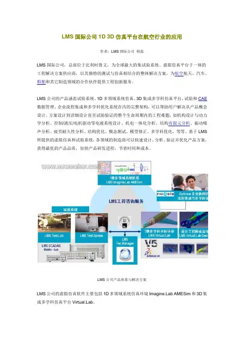
LMS国际公司1D3D仿真平台在航空行业的应用作者:LMS国际公司程磊LMS国际公司,总部位于比利时鲁文,为全球最大的集试验系统、虚拟仿真平台于一体的工程解决方案供应商,以其独特的测试与仿真相结合的整体解决方案,为航空航天、汽车、船舶和其它制造领域的合作伙伴提供工程创新服务。
LMS公司的产品涵盖试验系统、1D多领域系统仿真、3D集成多学科仿真平台、试验和CAE 数据管理、企业流程集成和多学科优化系统在内的完整架构,可以帮助用户解决从产品概念设计、方案设计到详细设计直至试验验证的整个生命周期内的工程难题,如机构设计与动力学分析、控制/液压/电机驱动等电液系统设计、机电一体化分析、结构有限元分析、振动噪声分析、疲劳耐久性分析、结构优化、模态测试、模型修正、多学科优化,等等。
基于LMS 所提供的虚拟仿真和试验系统,各领域的制造商可以快速设计、分析、验证并优化产品方案,获得最优的产品品质,加快产品研发进程,节省时间和成本。
LMS公司产品体系与解决方案LMS公司的虚拟仿真软件主要包括1D多领域系统仿真环境bAMESim和3D集成多学科仿真平台b。
bAMESim是当前CAE领域应用最为广泛的一维多领域仿真平台,它基于动态建模方法建立物理元件的数学模型,提供面向众多学科领域的专业应用库,包括控制、液压、气动、热、多相流、空调与冷却系统、电子电力、电磁、机械与动力传动、车辆动力学、内燃机,等等。
这些专业库和库元件都经过了大量工程检验。
用户只需要根据系统组成,把来自各专业库的预定义好的物理元件模型连接和组装起来,即可创建完整的系统模型,AMESim可自动形成系统方程,并进行稳态、瞬态或频响计算,分析系统性能;通过AMESim 集成的参数研究与优化工具或LMS公司专业的多学科优化系统Optimus,用户可以进一步对系统参数进行优化,找到达到产品设计目标的最优设计方案。
多领域系统仿真技术与AMESim平台,非常适合在产品方案设计阶段,在获得详细的几何模型前,进行整体方案设计和选型。
Virtual.lab声固耦合的隔声量仿真分析教程
FEM Direct Vibro-Acoustic Analysis Case TutorialObjective:The goal of this tutorial is to calculate the acoustic response of a glass/PVB plate (a laminated safety glass with a Polyvinyl butyral layer in between)・The tutorial includes using the following analysis cases:•Structural Modal case•Direct Structural Forced Response•Direct Structural Vibro-Acoustic Response•Transmission LossThe model contains a Visco-elastic frequency-dependent material・Pre-Requisites:Software Configurations that are needed to run the tutorial:•Licenses to set up the case in LMS b:u Desktop (VL-HEV.21.1 or equivalent)1' and "FiniteElement Acoustics (VL-"•When solving the acoustic response case, the license for product U LMS b FEM Vibro-Acoustics Structural Solver VL-VAM.45.2” is needed・•Solving the Random Post-processing case to get the T「ansmission Loss curve will require the license for n Random Vibro Acoustic Analysis (VL-nTutorial Data Files:StructuralGroups ・ xmlSAFyoung ・ xlsLaminatedStructure ・bdfFPmesh ・bdfAMLsender ・ bdfAMLreceiver ・bdfAcousticGroups ・ xml[All data files can be found on the APPS n DOCS DVD, in an archive called VAM_DirectVA-TL. For ease of use, it is best to copy all files to a local folder.]STEP BY STEP Tutorial:STEP 1After starting LMS b, create a new document in the Acoustic Harmonic FEMWorkbench (Start -^Acoustics -^Acoustic Harmonic FEM).STEP 2Select File -^Import from the main menu ・[The Import comma nd can also be selected from the con textualmenu of the Links Man ager, by right clicking]A file selector window appears allowing you to specify the file type and the file name・[For more details, see ]Select the file type NASTRAN Bulk File (匸bdf, *・NS# ^.nas f \dat) and browse for the file Laminatedstructure ・bdf and click the Open butt on. A new dialog box appears requesting the selection of data that needs to be imported from the file. The data entries that are not available in the file are grayed out. Select in Split into Multiple Mesh Pa「tsun der Mesh Creation and set the unit system to Meter, Kilogram, Second, click the OK buttOn.STEP 3Next, the d iff ere nt structural materials will be defined ・ The two outer layers of the panel are made of Glass ・To in corporate the 2% structural dampi ng of this material, it will be modeled as a viscoelastic material with a constant complex You ng modulus ・ The inner layer is made of PVB.Insert -^Materials -^New Materials -^New Viscoelastic Material...[Right-click on the Materials feature in the Specification Tree -^New Materials -^New Viscoelastic Material] Define the materials as follows:The PVB material at the center of the windshield has strong frequency dependent stiffness properties and is n early in compressible ・ The frequency depe ndency can be in corporated in a viscoelastic material using an edited load function. The values can be imported from the Excel document SAFyoung.xls as follows:Check Frequency Dependent, and right-click the input field・Select New Function・In the Attributes tab, enter as Name Young" s modulus PVB・In the Values tab, click the Import a file button, and browse to the excel file to select it.Switch the Data Format to Linear AmpHtude/Phase (deg) because the file contains the values like that. Click the Import butt on.Click the OK button of the Function Editor GULClick the OK button on the Material GULOn the Edited Load Function Set, create (usi ng the con text menu) a 2D display & type Comp/ex (Edited Load Function) on the Young's modulus and check the curve:STEP 4Defining two Structural 3D properties for Glass and PVB, applied to the structural groups Glass (with the defined material Glass) and PVB (with the defined material PVB).Insert -^Properties -^New Structural Properties -^Create 3D-Property[Right-click on the Properties feature in the Specification Tree-^- New Structural Properties -^•Create 3D-Property]Before the following steps please make sure the Mesh Parts are defined as types:PROPERTY0 一StructuralGlass 一StructuralPVB 一StructuralThis can be done by going to Tools -^Set Mesh Parts Type[Right-click on the mesh in the Specification Tree, Set Mesh Part Type -^Set as Structural Mesh Part]STEP 5In the next step, the model mesh will be imported from two Nastra n in put files ・ They each contain a mesh on which we will apply an AML property (Automatically Matched Layer), one on the receiver side, and one on the sender side.:File -^Import Acoustic Mesh -^Model Mesh..., and select the file AMLreceiver .bdfUse Meter, Kilogram and Seconds un its, and in elude the materials and properties ・Similarly, import AMLsender ・bdf ・At this point the mesh parts type definition window should look like this:STEP 6Inserting the New Material and properties for the new imported meshesInsert a new Acoustic material as follows (use the default values for air):Insert also a New Fluid Propert y. Call it also air, use the just defined material 'Air', and apply it to the two Acoustic mesh parts (Sender and Receiver side).STEP 7To facilitate the creation of the structural and acoustic model, some element groups have been predefined in xml files・ To import these groups, first create mesh group sets・Insert a New Group Set, either from the contextual menu or with Insert -^Mesh Grouping -^•Group Set....By right clicking the Group Set feature in the Specification Tree, insert a mesh group named Structural Groups, and in it import the 5 groups from the file structuralGroups ・ xml ・Right-click the Group Set, and use Mesh Grouping -^Group Selection Dialog...:Similarly insert a mesh group named Acoustic Groups, and in it import the 4 groups from the file AcousticGroups ・ xmlRight-click the group set, and use again Mesh Grouping ->Group Selection Dialog...:Step 8Save the analysis, but without closing.SETTING UP THE ACOUSTIC CASESStep 1Insert a new acoustic automatically matched layer property to take into account the semi-infinite extent of the sender and receiver rooms・ Insert a new AML property by right-clicking Properties, use New Acoustic Properties -^Automatically Matched Layer Property....Apply it to the two Acoustic groups AML Receiver and AML Sender. Switch the Radiation surface to User Defined, and select the AML Receiver group・Step 2Insert a Direct Vibro・Acoustic Response Analysis Case to compute the structural response and acoustic pressure fields in both the sender and receiver acoustic domains for each of the distributed plane wave excitations:To perform this calculation use No Load function Set and No Load Vector Set.Create new sets for all the rest.STEP 3Expand the Direct Vibro・Acoustic Response Analysis Case from the Specification Tree, right-click theBoundary Condition Set and use Acoustic Sources -^Distributed Plane Waves... with a Refinement Leveled 2, a Radius & 4m, and an Acoustic Pressure on lPa. The plane waves will be used to excite the system and to calculate the transmission loss characteristics of the panel.Since the panel is not aligned with the xy plane, this coordinate plane cannot be used to define the location of the plane wave sources・ So, for the Half Space Plane select Plane defined by Groups nd select the acoustic group coupling sender ・Select the Negative Half Space side.Click the OK butt on to gen erate a set of 12 spatially distributed plane waves ・By now the model should look similar to this:Step 4We will now restrain the border of the glass panel.Right-click the Restraint Set, add an Advanced Restraint QV\ the 3 Translational DOFs, and use as support the Structural Group BCs.Step 5Coupling surface definition will be used to couple the upper and lower surfaces of the panel to the envelope surface of the acoustic cavity・ When setting the Coupling Surface, the coupling between the structure and the fluid is on both sides.To correctly define the two-sided coupling in a transmission loss calculation, two coupling surfaces need to be created・ From the Coupling Surface Set.1 feature, double-click the Coupling Surface Set.1, and add the two surfaces: Structural Group CouplingSender and Acoustic Group Coupling Sender. Use a toleranee of 10mm and select as Coupling Type One side. Click the Apply button.Do the same for the Receiver Side in the end you should have two Coupling surfaces:Step 6Double-click on the Direct Vibro-Acoustic Response solution to update the analysis parameters. In the current tutorial, the response at the center frequencies of the third octave bands between 160Hz and 2000Hz will be analyzed・ In the Result Specifications tab, select User Defined for the Argument Axis Defin ition and remove the stan da rd an alysis freque ncy range・ Add a new frequency「ange definition and select a Logarithmic Step definition with a starting frequency of 160Hz, an ending frequency of 2000Hz and a step of 1 ・ 8. Click the OK butt on to add the frequency「ange defi nition.Request lector results at Field Points and for the Acoustic Potentials. No need to solve for Structural Displacements for now・Adjust the Solving Parameters・If your system is set up for parallel processing (see the Advaneed Acoustic Installation manual), try one of the Parallelism types・ Use the Direct solver.Adjust also the Job and Resources, e.g. to use multiple threads・Leave the Output Sets empty, meaning that results will be computed wherever possible.Step 7Update the Direct Vibro-Acoustic Response Solution to compute the acoustic pressure fields and structural deformations. This will take a while, as there are 23 frequencies and 12 load conditions. Save your model.Step 8Displaying the resultsOnce the computation is finished, right-click the Direct Vibro-Acoustic Response Solution Set.l feature and select Generate Image from the con textual menu ・[or select the solution feature and click the Gen erate Image toolbar butt on.]The Image Generation dialog box will appear, select the Pressure.Double-click the image feature in the Specification Tree, and in the Occurrences tab select the for example thefirst Load Condition (meaning the loading by the first distributed plane wave source) and set the freque ncy at 508Hz, click the OK butt on. For b etter visualizati on you can hide the Nodes and Elements feature, and the Boundary Conditions feature (with its plane wave sources)・You can also display the 2D image curve for the Acoustic Power on the Kirchhoff surfaceRight-click the Direct Vibro-Acoustic Response Solution Set.1 feature and select New Function Display..・from the con textual menu. The New Function Display dialog box will appear requesting you to select the different display images・[Also you can use the 匸button from the toolbar and select the Solution Set feature. A third possibility is to use the menu Insert ->2D/3D Images ->New Function Display] Select the 2D Display from the list and click the Finish button.A new window, containing X- and Y-axes along with the Select Data dialog box will now appear. In the Select Data dialog box, select Kirchhoff Surface Radiation: Sand click the Display button As each of the distributed plane wave sources are independent, the sound power can be obtained by simply adding the individual contributions・ So, select all 12 Data cases, and check the option Sum over data cases・Switch the x-axis format to Octaves, and the Y-axis to dB(RMS). You can use dot markers for the curve by right-clicki ng it, using the Opti ons …command in its con text menu, and the n changing the settings in the Visualization tab・Save your modelStep 9To get the transmission loss curve, we need to divide the total acoustic power on the receiver side by the total power on the sender side. Before we can do that, we need to combine the individual cases (one for each distributed plane wave source) to get the total power curves・Insert a Random Post-processing Case with Insert ->Other Analysis Cases -^-Random Post-Processing Case...Refer to the solution of the previous response case, and select to process for a Cross Power Set with Unitary Uncorrelated Load Cases:Update its solution using the context menu on its solution feature Random Response Solution Set.X. This will go fast.Right-click the sub-solution Global Indicator Set.X and create a New Function Display QV\ it. Select the 2D Display as seenario, and click the Finish button.A 2D display window will appear with the Select Data dialog box open. In the General tab, switch the drop-down selector to Transmission Loss, and select the entry Coupled Surfaced and click the Display button.You can see a TL value of 30.461911 dB for the 319.996 Hz octave band:Theory for Panel Transmission LossCalculation of Transmission Loss using Vibro-Acoustic FEMThis topic describes how to set up a model and the computation to compute the Transmission Loss (e.g・ for a panel) using the LMS b tools・Stepl ・Import of an Acoustic and Structural meshand a structural mesh with the modal data in the Acoustic Harmonic FEM workbench・ There is no need to have a field point mesh.Step2. Create a New Acoustic PropertyDefine the Acoustic Properties jn eluding fluid properties a nd possible impedance g the panel. Create an property for the source room on all faces that are not coupled to the panel and not touching the joined wall. The wall must be a zero velocity boundary condition. Also create an Automatically Matched Layer (AML) on the an echoic room side, which is defi ned as a Kirchhoff surface ・Step3. Insert the boundary conditionCreate an acoustic boundary condition by selecting Insert -^Acoustic Boundary Conditions and Sources -^Acoustic Boundary Condition and Source Set... from the main menu. The Boundary Condition Set Creation dialog box appears as shown in the image below:Click the OK button to close the dialog box. A new Acoustic Boundary Conditions and Sources feature appears in the Specification Tree as shown in the image below:Now, similarly add to the Acoustic Boundary Condition and Sources an acoustic source of type in the source 「oom.Step4. Insert a Vibro-Acoustic Response and Random Post-Processing Analysis CaseInsert the Modal-based by selecting Insert -^FEM Analysis Cases -^Modal Based Vibro -Acoustic Response Analysis Case..・from the main menu, or click the Create a Modal Based Vibro-Acoustic Response Analysis Case...麹butto n from the FEM Analysis Cases toolbar. Define the Mesh Mapping and select the structural shells and the two groups of acoustic faces (one in the source room and one in the receiver room). Compute the Modal-based Vibro-Acoustic Response Analysis case・ It will compute the Incident Power and the Radiated Power for each source・Similarly, insert a z and Compute it. It will compute the Total Powers a nd store it in a sub-solution called Global Indicator Set as:•Total Incident Power, having Physical Type as INPUT^POWER and Response ID as Coupled Surfaced.•Total Power radiated by the Acoustic Mesh, having Physical Type as ACOUSTIC_POWER andResponse ID as Kirchhoff Surface Radiation:S.• If you have a field point mesh which is not needed to compute the Transmission Loss), it will alsocompute the Total Power on the Field Point Mesh having Physical Type as ACOU5TIC_POWER andResponse ID as Field Point Mesh:S.The Random Response Solution ^computes also the Transmission £055 with the following formula:Where,is the Incident Power^out is the Radiated PowerSt 即5: Post-ProcessingStandard results will be post-processed on the analysis cases.The Incident Power, Radiated Power a nd Transmission Loss are stored as Expressions, Load Functions by the Global Indicator Set, and can be displayed in a 2D Function Display.The Transmission Loss will be stored with Physical Type as "ABSORPTIVITY"and Response ID as "Coupled Surface:S,rManual calculation of Transmission Loss by using Edited Load FunctionStepl. Insert an ・To insert an Edited Load Function, select from the main menu Insert -^Functions Creator ■^■Edited Load Function... or use the Create an Edited Load Function ^^button available in the Functions Creator toolbar・Step2. Import Kirchhoff Surface Radiation :S fu nction from Global Indicators of the Random Post-Processing Solution Set of the Acoustic document. Take only the Rea/Part.Step3. Again, import the function Acoustic Power on Field Point Mesh:S from Global Indicators of the Random Post-Processing Solution Set of the Structural document. Take only the Real Part and Amplitude of that Part. Step4. Multiply this function with 0.5. As the actual incident power is half the power through the field point mesh. This is because the in cident pressure is imposed as total pressure on the wall.Step5 ・Now, divide these two fun ctions and take the Log of that function and fin ally multiply it with 10.Step6.To visualize the computed Transmission Loss, right-click the Edited load function in the Specification Tree and select the New Function Display..・opti on from the con textual menu ・ Select 2D Display from the list and click the Finish button. From the Select Data dialog box select Transmission Loss using the drop-down menu. BEM Symmetry Plane SetThe mathematical formulation of the Boundary Element method leads to dense matrices, with the con sequence that a lin ear increase in model size N (number of nodes and elements, or more gen erally, nu mber of DOFs) leads toA parabolic increase (order N**2) for the BEM matrix storage requirementsA cubic increase (order N**3) for the BEM matrix solution timeTherefore, it is very advantageous to exploit symmetry characteristics in the geometry of the sound-radiating structure to the full extend. If you need to model only one-half, one-quarter or one-eighth of a vibrating structure, this leads to a drastic reduction in memory requirements and solution time for the problem at hand・The Symmetry Plane Set comma nd allows you to defi ne the acoustical symmetry or anti-symmetry conditionswith respect to planes that are parallel to the coordinate axis planes (XY, YZ or XZ). The Symmetry Plane or Baffle will be correctly visualised, if the Mesh is Acoustic (Mesh Type: Acoustic) and a Mesh Preprocessing Set is inserted in the Specification Tree・To insert a new Symmetry Plane Set, click the Insert/Edit a Symmetry Plane Set button in the Acoustic Model Definition toolbar or select Insert -^Symmetry Plane Set from the main menu. A new dialog box will appear as shown in the image below・Figure: Symmetry and Anti-Symmetry Plane dialog• Planes X, Y and ZThese planes are defi ned by their position along the perpe ndicular di recti on with respect to thecoordinate axis plane; for instan ce, the X-symmetry plane X=1000mm defines a symmetry plane parallel to the YZ plane and passing through the point (1000,0,0)・Although the geometry should always be symmetrical in order to allow the definition of symmetry andanti-symmetry planes, the actual acoustical conditions can be symmetrical (identical) or anti-symmetrical (opposite) with respect to the plane depending on the type of plane selected・ The following tablesummarizes the effect of defining symmetrical or anti-symmetrical conditions for both acoustical andstructural boundary conditions:Figure: Symmetry and Anti-Symmetry conditions summaryUp to three mutually perpendicular symmetry or anti-symmetry planes can be defined simultaneous!y.Of course, only one symmetry or anti-symmetry plane can be defined parallel to each coordinate axisplane XY, YZ or XZ・Since acoustical symmetry implies zero normal velocity, defining a symmetry plane is acousticallyequivalent to the presence of a rigid, 100% reflecting floor・In other words, if you are modeling a situation where the sound-radiating structure is located on a hard floor, e.g. the concrete floor of asemi-anechoic chamber, the presence of this floor can be represented simply by a symmetry plane.Conversely, since acoustical anti-symmetry implies zero acoustic pressure, defining an anti-symmetryplane is acoustically equivalent to the presence of pressure release surface・This kind of surface can be used to model free surfaces like a water-air interface. E.g., if you need to model the acousticradiati on into water from a submarine at a certain depth, you can model the presence of the seasurface above the submarine by defining an anti-symmetry plane.When defining these kinds of planes, they are represented by colored square surfaces. You can also change the colors of the planes by selecting Tools -^Options AcousticsDisplay tab.•By default, symmetry planes are represented by semi-transparent bright green squares with anopaque border as shown in the image below・•By default, anti-symmetry planes are represented by semi-transparent bright blue squares with anopaque border as shown in the image below・The presenee of these surfaces will also have an important impact on the type of boundary conditions that are created by the Acoustic Mesh Preprocessing operation.•BaffleThis functionality is useful for handling the acoustic transparency problems and allows you to computethe insertion or transmission loss. It is only available in the Acoustic Harmonic BEM Workbench when the model type is Indirect type. The baffle is represented as a symmetry plane but with red color as shown in the image below・The Transmission loss and Insertion loss can be computed in term of pressure or acoustic power. This is quite straightforward when it is done on the pressure, but some postprocessing is needed when it is done on the power・ The Incident Power and Transmitted Power can be calculated by using the following formulae・Incident PowerUsually for the transmission loss computation, an acoustic diffuse field is defined on one side of the baffle・ The Incident Power can be computed with the following formula:where Prms is the diffuse field acoustic RMS pressure and S is the surface of the structure impacted by the incident diffuse field・ This is valid for a diffuse field generated by a sum of plane waves ・ The total in put power is the sum of the individual source power. This can be easily computed in an edited load function・Transmitted PowerThe Transmitted Power can be computed by defining a hemispherical field point mesh almost touching the baffle and computing the field response. The total Transmitted Power will then be computed in the「andom post processing case・ When updating the solution, if there is acoustic power through field point mesh available in the in put solutio n, the total acoustic power will be computed with the following equation:where Wt is the total acoustic power, NLC is the number of pseudo load-cases, 5 are the singular values (Virtual Autopowers) and Wi is the acoustic power for load case i.。
Virtual.lab声固耦合的隔声量仿真分析教程
FEM Direct Vibro-Acoustic Analysis Case Tutorial Objective:The goal of this tutorial is to calculate the acoustic response of a glass/PVB plate (a laminated safety glass with a Polyvinyl butyral layer in between).The tutorial includes using the following analysis cases:∙Structural Modal case∙Direct Structural Forced Response∙Direct Structural Vibro-Acoustic Response∙Transmission LossThe model contains a Visco-elastic frequency-dependent material.Pre-Requisites:Software Configurations that are needed to run the tutorial:∙Licenses to set up the case in LMS b: "Desktop (VL-HEV.21.1 or equivalent)"and "Finite Element Acoustics (VL-VAM.36.2)"∙When solving the acoustic response case, the license for product "LMS bFEM Vibro-Acoustics Structural Solver VL-VAM.45.2" is needed.∙Solving the Random Post-processing case to get the Transmission Loss curve willrequire the license for "Random Vibro Acoustic Analysis (VL-NVP.20.3)"Tutorial Data Files:StructuralGroups.xmlSAFyoung.xlsLaminatedStructure.bdfFPmesh.bdfAMLsender.bdfAMLreceiver.bdfAcousticGroups.xml[All data files can be found on the APPS n DOCS DVD, in an archive called VAM_DirectVA-TL. For ease of use, it is best to copy all files to a local folder.]STEP BY STEP Tutorial:STEP 1After starting LMS b, create a new document in the Acoustic Harmonic FEM Workbench (Start Acoustics Acoustic Harmonic FEM).STEP 2Select File Import from the main menu. [The Import command can also be selected from the contextual menu of the Links Manager, by right clicking]A file selector window appears allowing you to specify the file type and the file name. [For more details, see Importing Data]Select the file type NASTRAN Bulk File (*.bdf, *.NS, *.nas, *.dat) and browse for the file LaminatedStructure.bdf and click the Open button. A new dialog box appears requesting the selection of data that needs to be imported from the file. The data entries that are not available in the file are grayed out.Select in Split into Multiple Mesh Parts under Mesh Creation and set the unit system to Meter, Kilogram, Second, click the OK button.STEP 3Next, the different structural materials will be defined. The two outer layers of the panel are made of Glass. To incorporate the 2% structural damping of this material, it will be modeled asa viscoelastic material with a constant complex Young modulus. The inner layer is made of PVB.Insert Materials New Materials New Viscoelastic Material...[Right-click on the Materials feature in the Specification Tree New Materials New Viscoelastic Material]Define the materials as follows:The PVB material at the center of the windshield has strong frequency dependent stiffness properties and is nearly incompressible. The frequency dependency can be incorporated in a viscoelastic material using an edited load function. The values can be imported from the Excel document SAFyoung.xls as follows:Check Frequency Dependent, and right-click the input field.Select New Function.In the Attributes tab, enter as Name Young’s modulus PVB.In the Values tab, click the Import a file button, and browse to the excel file to select it.Switch the Data Format to Linear Amplitude/Phase (deg) because the file contains the values like that. Click the Import button.Click the OK button of the Function Editor GUI.Click the OK button on the Material GUI.On the Edited Load Function Set, create (using the context menu) a 2D display of type Complex(Edited Load Function) on the Young’s modulus and check the curve:STEP 4Defining two Structural 3D properties for Glass and PVB, applied to the structural groups Glass (with the defined material Glass) and PVB (with the defined material PVB).Insert Properties New Structural Properties Create 3D-Property[Right-click on the Properties feature in the Specification Tree New Structural Properties Create 3D-Property]Before the following steps please make sure the Mesh Parts are defined as types:PROPERTY0 – StructuralGlass – StructuralPVB – StructuralThis can be done by going to Tools Set Mesh Parts Type[Right-click on the mesh in the Specification Tree, Set Mesh Part Type Set as Structural Mesh Part]STEP 5In the next step, the model mesh will be imported from two Nastran input files. They each contain a mesh on which we will apply an AML property (Automatically Matched Layer), one on the receiver side, and one on the sender side.:File Import Acoustic Mesh Model Mesh..., and select the file AMLreceiver.bdf Use Meter, Kilogram and Seconds units, and include the materials and properties. Similarly, import AMLsender.bdf.At this point the mesh parts type definition window should look like this:STEP 6Inserting the New Material and properties for the new imported meshesInsert a new Acoustic material as follows (use the default values for air):Insert also a New Fluid Property. Call it also air, use the just defined material 'Air', and apply it to the two Acoustic mesh parts (Sender and Receiver side).STEP 7To facilitate the creation of the structural and acoustic model, some element groups have been predefined in xml files. To import these groups, first create mesh group sets.Insert a New Group Set, either from the contextual menu or with Insert Mesh Grouping Group Set....By right clicking the Group Set feature in the Specification Tree, insert a mesh group named Structural Groups, and in it import the 5 groups from the file StructuralGroups.xml. Right-click the Group Set, and use Mesh Grouping Group Selection Dialog…:Similarly insert a mesh group named Acoustic Groups, and in it import the 4 groups from the file AcousticGroups.xmlRight-click the group set, and use again Mesh Grouping Group Selection Dialog…:Step 8Save the analysis, but without closing.SETTING UP THE ACOUSTIC CASESStep 1Insert a new acoustic automatically matched layer property to take into account thesemi-infinite extent of the sender and receiver rooms. Insert a new AML property byright-clicking Properties, use New Acoustic Properties Automatically Matched Layer Property....Apply it to the two Acoustic groups AML Receiver and AML Sender. Switch the Radiation surface to User Defined, and select the AML Receiver group.Step 2Insert a Direct Vibro-Acoustic Response Analysis Case to compute the structural response and acoustic pressure fields in both the sender and receiver acoustic domains for each of the distributed plane wave excitations:To perform this calculation use No Load function Set and No Load Vector Set.Create new sets for all the rest.STEP 3Expand the Direct Vibro-Acoustic Response Analysis Case from the Specification Tree, right-click the Boundary Condition Set and use Acoustic Sources Distributed Plane Waves... with a Refinement Level of 2, a Radius of4m, and an Acoustic Pressure on 1Pa. The plane waves will be used to excite the system and to calculate the transmission loss characteristics of the panel.Since the panel is not aligned with the xy plane, this coordinate plane cannot be used to define the location of the plane wave sources. So, for the Half Space Plane select Plane defined by Group and select the acoustic group Coupling Sender.Select the Negative Half Space side.Click the OK button to generate a set of 12 spatially distributed plane waves.By now the model should look similar to this:Step 4We will now restrain the border of the glass panel.Right-click the Restraint Set, add an Advanced Restraint on the 3 Translational DOFs, and use as support the Structural Group BCs.Step 5Coupling surface definition will be used to couple the upper and lower surfaces of the panel to the envelope surface of the acoustic cavity. When setting the Coupling Surface, the coupling between the structure and the fluid is on both sides.To correctly define the two-sided coupling in a transmission loss calculation, two coupling surfaces need to be created. From the Coupling Surface Set.1 feature, double-click the Coupling Surface Set.1, and add the two surfaces: Structural Group CouplingSender and Acoustic Group Coupling Sender. Use a tolerance of 10mm and select as Coupling Type One side. Click the Apply button.Do the same for the Receiver Side in the end you should have two Coupling surfaces:Step 6Double-click on the Direct Vibro-Acoustic Response solution to update the analysis parameters. In the current tutorial, the response at the center frequencies of the third octave bands between 160Hz and 2000Hz will be analyzed. In the Result Specifications tab, select User Defined values for the Argument Axis Definition and remove the standard analysis frequency range. Add a new frequency range definition and select a Logarithmic Step definition with a starting frequency of 160Hz, an ending frequency of 2000Hz and a step of 1.122462048. Click the OK button to add the frequency range definition.Request Vector results at Field Points and for the Acoustic Potentials. No need to solve for Structural Displacements for now.Adjust the Solving Parameters. If your system is set up for parallel processing (see the Advanced Acoustic Installation manual), try one of the Parallelism types. Use the Direct solver.Adjust also the Job and Resources, e.g. to use multiple threads.Leave the Output Sets empty, meaning that results will be computed wherever possible.Step 7Update the Direct Vibro-Acoustic Response Solution to compute the acoustic pressure fields and structural deformations. This will take a while, as there are 23 frequencies and 12 load conditions. Save your model.Step 8Displaying the resultsOnce the computation is finished, right-click the Direct Vibro-Acoustic Response Solution Set.1 feature and select Generate Image from the contextual menu.[or select the solution feature and click the Generate Image toolbar button.]The Image Generation dialog box will appear, select the Pressure.Double-click the image feature in the Specification Tree, and in the Occurrences tab select the for example the first Load Condition (meaning the loading by the first distributed plane wave source) and set the frequency at 508Hz, click the OK button. For better visualization you can hide the Nodes and Elements feature, and the Boundary Conditions feature (with its plane wave sources).You can also display the 2D image curve for the Acoustic Power on the Kirchhoff surfaceRight-click the Direct Vibro-Acoustic Response Solution Set.1feature and select New Function Display... from the contextual menu. The New Function Display dialog box will appear requesting you to select the different display images.[Also you can use the button from the toolbar and select the Solution Set feature. A third possibility is to use the menu Insert 2D/3D Images New Function Display]Select the 2D Display from the list and click the Finish button.A new window, containing X- and Y-axes along with the Select Data dialog box will now appear. In the Select Data dialog box, select Kirchhoff Surface Radiation: S and click the Display buttonAs each of the distributed plane wave sources are independent, the sound power can be obtained by simply adding the individual contributions. So, select all 12 Data Cases, and check the option Sum over data cases.Switch the x-axis format to Octaves, and the Y-axis to dB(RMS). You can use dot markers for the curve by right-clicking it, using the Options... command in its context menu, and then changing the settings in the Visualization tab.Save your modelStep 9To get the transmission loss curve, we need to divide the total acoustic power on the receiver side by the total power on the sender side. Before we can do that, we need to combine the individual cases (one for each distributed plane wave source) to get the total power curves.Insert a Random Post-processing Case with Insert Other Analysis Cases Random Post-Processing Case...Refer to the solution of the previous response case, and select to process for a Cross Power Set with Unitary Uncorrelated Load Cases:Update its solution using the context menu on its solution feature Random Response Solution Set.X. This will go fast.Right-click the sub-solution Global Indicator Set.X and create a New Function Display on it. Select the 2D Display as scenario, and click the Finish button.A 2D display window will appear with the Select Data dialog box open. In the General tab, switch the drop-down selector to Transmission Loss, and select the entry Coupled Surface:S and click the Display button.You can see a TL value of 30.461911 dB for the 319.996 Hz octave band:Theory for Panel Transmission LossCalculation of Transmission Loss using Vibro-Acoustic FEMThis topic describes how to set up a model and the computation to compute the Transmission Loss (e.g. for a panel) using the LMS b tools.Step1.Import of an Acoustic and Structural meshImport an acoustic mesh and a structural mesh with the modal data in the Acoustic Harmonic FEM workbench. There is no need to have a field point mesh.Step2. Create a New Acoustic PropertyDefine the Acoustic Properties including fluid properties and possible impedance on the panel. Create an Automatically Matched Layer (AML) property for the source room on all faces that are not coupled to the panel and not touching the joined wall. The wall must be a zero velocity boundary condition. Also create an Automatically Matched Layer (AML) on the anechoic room side, which is defined as a Kirchhoff surface.Step3. Insert the boundary conditionCreate an acoustic boundary condition by selecting Insert Acoustic Boundary Conditions and Sources Acoustic Boundary Condition and Source Set… from the main menu. The Boundary Condition Set Creation dialog box appears as shown in the image below:Click the OK button to close the dialog box. A new Acoustic Boundary Conditions and Sources feature appears in the Specification Tree as shown in the image below:Now, similarly add to the Acoustic Boundary Condition and Sources an acoustic source of type Distributed Plane Waves in the source room.Step4. Insert a Vibro-Acoustic Response and Random Post-Processing Analysis CaseInsert the Modal-based Vibro-Acoustic Response Analysis Case by selecting InsertFEM Analysis Cases Modal Based Vibro-Acoustic Response Analysis Case… from the main menu, or click the Create a Modal Based Vibro-Acoustic Response AnalysisCase… button from the FEM Analysis Cases toolbar. Define the Mesh Mapping and selectthe structural shells and the two groups of acoustic faces (one in the source room and one in the receiver room). Compute the Modal-based Vibro-Acoustic Response Analysis case. It will compute the Incident Power and the Radiated Power for each source.Similarly, insert a Random Post-Processing Case, and Compute it. It will compute the Total Powers and store it in a sub-solution called Global Indicator Set as:∙Total Incident Power, having Physical Type as INPUT_POWER and Response ID asCoupled Surface:S.∙Total Power radiated by the Acoustic Mesh, having Physical Type asACOUSTIC_POWER and Response ID as Kirchhoff Surface Radiation:S.∙If you have a field point mesh which is not needed to compute the Transmission Loss), it will also compute the Total Power on the Field Point Mesh having Physical Type asACOUSTIC_POWER and Response ID as Field Point Mesh:S.The Random Response Solution Set computes also the Transmission Loss with the following formula:Where,is the Incident Poweris the Radiated PowerStep5: Post-ProcessingStandard results will be post-processed on the analysis cases.The Incident Power, Radiated Power and Transmission Loss are stored as Expressions, Load Functions by the Global Indicator Set, and can be displayed in a 2D Function Display.The Transmission Loss will be stored with Physical Type as "ABSORPTIVITY" and Response ID as "Coupled Surface:S"Manual calculation of Transmission Loss by using Edited Load FunctionStep1.Insert an Edited Load Function.To insert an Edited Load Function, select from the main menu Insert Functions CreatorEdited Load Function… or use the Create an Edited Load Function button available in the Functions Creator toolbar.Step2.Import Kirchhoff Surface Radiation:S function from Global Indicators of the Random Post-Processing Solution Set of the Acoustic document. Take only the Real Part.Step3. Again, import the function Acoustic Power on Field Point Mesh:S from Global Indicators of the Random Post-Processing Solution Set of the Structural document. Take only the Real Part and Amplitude of that Part.Step4. Multiply this function with 0.5. As the actual incident power is half the power through the field point mesh. This is because the incident pressure is imposed as total pressure on the wall.Step5. Now, divide these two functions and take the Log of that function and finally multiply it with 10.Step6.Create a 2D displayTo visualize the computed Transmission Loss, right-click the Edited load function in the Specification Tree and select the New Function Display… option from the contextual menu. Select 2D Display from the list and click the Finish button. From the Select Data dialog box select Transmission Loss using the drop-down menu.BEM Symmetry Plane SetThe mathematical formulation of the Boundary Element method leads to dense matrices, with the consequence that a linear increase in model size N (number of nodes and elements, or more generally, number of DOFs) leads toA parabolic increase (order N**2) for the BEM matrix storage requirementsA cubic increase (order N**3) for the BEM matrix solution timeTherefore, it is very advantageous to exploit symmetry characteristics in the geometry of the sound-radiating structure to the full extend. If you need to model only one-half, one-quarter or one-eighth of a vibrating structure, this leads to a drastic reduction in memory requirements and solution time for the problem at hand.The Symmetry Plane Set command allows you to define the acoustical symmetry oranti-symmetry conditions with respect to planes that are parallel to the coordinate axis planes (XY, YZ or XZ). The Symmetry Plane or Baffle will be correctly visualised, if the Mesh is Acoustic (Mesh Type: Acoustic) and a Mesh Preprocessing Set is inserted in the Specification Tree.To insert a new Symmetry Plane Set, click the Insert/Edit a Symmetry Plane Set button in the Acoustic Model Definition toolbar or select Insert Symmetry Plane Set from the main menu. A new dialog box will appear as shown in the image below.Figure: Symmetry and Anti-Symmetry Plane dialogPlanes X, Y and ZThese planes are defined by their position along the perpendicular direction withrespect to the coordinate axis plane; for instance, the X-symmetry plane X=1000mm defines a symmetry plane parallel to the YZ plane and passing through the point(1000,0,0).Although the geometry should always be symmetrical in order to allow the definition of symmetry and anti-symmetry planes, the actual acoustical conditions can besymmetrical (identical) or anti-symmetrical (opposite) with respect to the planedepending on the type of plane selected. The following table summarizes the effect of defining symmetrical or anti-symmetrical conditions for both acoustical and structural boundary conditions:Figure: Symmetry and Anti-Symmetry conditions summaryUp to three mutually perpendicular symmetry or anti-symmetry planes can be defined simultaneously. Of course, only one symmetry or anti-symmetry plane can be defined parallel to each coordinate axis plane XY, YZ or XZ.Since acoustical symmetry implies zero normal velocity, defining a symmetry plane is acoustically equivalent to the presence of a rigid, 100% reflecting floor. In other words, if you are modeling a situation where the sound-radiating structure is located on a hard floor, e.g. the concrete floor of a semi-anechoic chamber, the presence ofthis floor can be represented simply by a symmetry plane.Conversely, since acoustical anti-symmetry implies zero acoustic pressure, defining an anti-symmetry plane is acoustically equivalent to the presence of pressurerelease surface. This kind of surface can be used to model free surfaces like awater-air interface. E.g., if you need to model the acoustic radiation into water from a submarine at a certain depth, you can model the presence of the sea surface above the submarine by defining an anti-symmetry plane.When defining these kinds of planes, they are represented by colored square surfaces. You can also change the colors of the planes by selecting Tools Options AcousticsDisplay tab.∙By default, symmetry planes are represented by semi-transparent bright greensquares with an opaque border as shown in the image below.∙By default, anti-symmetry planes are represented by semi-transparent bright bluesquares with an opaque border as shown in the image below.The presence of these surfaces will also have an important impact on the type of boundary conditions that are created by the Acoustic Mesh Preprocessing operation.BaffleThis functionality is useful for handling the acoustic transparency problems and allows you to compute the insertion or transmission loss. It is only available in the AcousticHarmonic BEM Workbench when the model type is Indirect type. The baffle isrepresented as a symmetry plane but with red color as shown in the image below.The Transmission loss and Insertion loss can be computed in term of pressure or acoustic power. This is quite straightforward when it is done on the pressure, but some postprocessing is needed when it is done on the power. The Incident Power and Transmitted Power can be calculated by using the following formulae.Incident PowerUsually for the transmission loss computation, an acoustic diffuse field is defined on one side of the baffle. The Incident Power can be computed with the following formula:where Prms is the diffuse field acoustic RMS pressure and S is the surface of the structure impacted by the incident diffuse field. This is valid for a diffuse field generated by a sum of plane waves. The total input power is the sum of the individual source power. This can be easily computed in an edited load function.Transmitted PowerThe Transmitted Power can be computed by defining a hemispherical field point mesh almost touching the baffle and computing the field response. The total Transmitted Power will then be computed in the random post processing case. When updating the solution, if there is acoustic power through field point mesh available in the input solution, the total acoustic power will be computed with the following equation:where Wt is the total acoustic power, NLC is the number of pseudo load-cases, are the singular values (Virtual Autopowers) and Wi is the acoustic power for load case i.。
【参考文档】matlab实验心得体会_学习matlab的心得体会-优秀word范文(3页)
【参考文档】matlab实验心得体会_学习matlab的心得体会-优秀word范文(3页)本文部分内容来自网络整理,本司不为其真实性负责,如有异议或侵权请及时联系,本司将立即删除!== 本文为word格式,下载后可方便编辑和修改!== matlab 实验心得体会_学习matlab的心得体会导语:通过对MATLAB的系统环境,数据的各种运算,矩阵的分析和处理,程序设计,绘图,数值计算及符号运算的学习,初步掌握了MATLAB的实用方法。
以下是小编带来的matlab实验心得体会,希望对您有所帮助。
matlab实验心得体会(一)学习matlab是听说它是一个功能强大的数学软件,但是正被微积分的计算缠身,听说有一个高级的计算器当然高兴,以后可以偷懒了,当然现在不能偷懒。
听说关于自动化的计算特别复杂,如果有一种软件能帮忙解题,那是一种极大的解脱,有益于缩短研究时间。
目前我只知道有三种数学软件,都是国外的,没有国内的,差距挺大的。
matlab学起来挺顺手的,比C语言简单。
但是深入学习的时候却困难重重,因为很多知识都没有学习,就算知道那些函数,也没有什么用处。
老师布置的作业难度大,写一篇实验,大一什么都不会,写一篇这种论文谈何容易。
最多也就会一些数值计算、符号计算、简单绘图,根本不会什么实验。
学习matlab体会最多的是这个软件的功能强大,好多数学题都被轻易的解出。
但是有一点遗憾,不知是我不会用,还是它没个功能,已知空间的电荷分布,求空间的电场分布。
其中电场分布是无法用函数表达式表示。
我知道计算机肯定可以实现,但是这个软件能不能实现就不知道了,我看过许多资料,但是在这方面没有提到相关信息。
总之,这个软件功能强大,不知什么时候国内才有类似的软件。
matlab实验心得体会(二)我从中国石油大学(北京)来到大庆油田勘探开发研究院实习,刚刚来到这里时我内心充满了激动和喜悦,对这个有着辉煌成绩的科研单位充满了期待。
到了这里没多久我就参加培训中心组织的入院教育,对研究院的辉煌过去有了更深刻的了解,那时我就下定决心在研究院好好实习,多学习一些现场经验,为以后的工作打下良好的基础。
初学matlab报告心得
初学matlab报告心得引言MATLAB(Matrix Laboratory)是一种用于数值计算和数据可视化的高级软件系统。
作为一名初学者,我在学习MATLAB的过程中获得了许多宝贵的经验和体验,本报告将对此进行总结和分享。
学习经历学习资源选择在学习MATLAB之前,我首先通过互联网搜索了一些与MATLAB相关的学习资源。
这些资源包括MATLAB官方文档、教程视频以及在线论坛等。
经过仔细比较,我选择了一本深入浅出的MATLAB教程书籍作为我的主要学习资料。
这本书籍以简洁、通俗易懂的方式介绍了MATLAB的基础知识和常用功能,非常适合初学者。
学习方法在真正开始学习MATLAB之前,我制定了一套学习计划。
首先,我将学习材料中的每个章节进行分类,然后根据难易程度和相关性进行排序。
然后,我每天规划一定的学习时间,按照计划逐一学习每个章节的内容。
对于不熟悉的概念和方法,我会进行反复阅读,并尝试在MATLAB环境中实践。
学习心得通过学习MATLAB,我收获了许多宝贵的经验和体会。
首先,MATLAB的语法简洁而灵活,使得编写代码变得非常方便。
与其他编程语言相比,MATLAB具有更高的可读性和可理解性,对于初学者来说,减少了理解和调试的困难。
其次,MATLAB提供了丰富的工具箱和函数库,可以轻松完成各种数值计算和数据处理任务。
与传统的编程语言相比,MATLAB的内置函数和工具箱简化了代码的编写过程,提高了工作效率。
此外,MATLAB还具有强大的数据可视化能力。
通过简单的命令和函数,我们可以将数据以图表的形式展示出来,便于观察和分析。
这对于理解和解释数据非常有帮助。
最后,学习MATLAB需要不断的实践和尝试。
仅仅阅读书籍和文档是远远不够的,我们需要将所学内容应用到实际问题中,才能真正理解和掌握。
学习收获通过学习MATLAB,我不仅掌握了MATLAB的基础知识和常用功能,还培养了一些与编程相关的能力和思维方式。
首先,我学会了如何利用MATLAB进行数据处理和分析。
Matlab学习心得与体会
Only in boiling water, tea can develop the rich aroma of life.简单易用轻享办公(页眉可删)Matlab学习心得与体会Matlab学习心得与体会篇一:MATLAB学习心得一.对MATLAB的认识正如课本《MATLAB教程及实训》中的前言所说,MATLAB是MathWords公司于1984年开发的,目前已经发展成国际上最流行、应用最广泛的科学与工程计算软件之一。
MATLAB集合矩阵云运算、数值分析、图形显示和仿真等于一体,被广泛应用于自动控制、数学运算、计算机技术、图像信号处理、汽车工业、语音处理等行业。
MATLAB它将计算、可视化和编程等功能同时集于一个易于开发的环境。
MATLAB主要应用于数学计算、系统建模与仿真、数学分析与可视化、科学与工程制图和用户界面设计等。
目前,MATLAB已经成为应用代数、自动控制理论、数字信号处理、动态系统仿真和金融等专业的基本数学工具,各国高校纷纷将MATLAB正式列入本科生和研究生课程的教书计划中,成为学生必须掌握的软件之一。
MATLAB是matrix laboratory的缩写,它的产生是与数学计算有密切的关系。
从1980年发展到现在已经是一个交互式开发系统,其基本数据要素是矩阵。
MATLAB系统是由MATLAB开发环境和MATLAB语言,MATLAB数学函数库、MATLAB图形处理系统和MATLAB应用程序接口(APL)5部分组成。
MATLAB的有以下特点1运算功能强大 2编程效率高3强大而智能化的作图功能 4可扩展性强 5Simulink 动态仿真功能二.我对MATLAB的掌握程度在短课时选择了本书1、2、3、4、5、7章的内容学习1. MATLAB R20__a软件的概述(略)。
2. MATLAB常见字符及基本运算在本人的自主学习以及老师的授课下我已经初略的掌握了MATLAB R20__a的基本使用方法:MATLAB R20__a的开发环境、MATLAB R20__a的其他管理、MATLAB的文件处理工具、MATLAB R20__a的帮助系统(1)数据类型数组:字符型、数值型、元胞型、结构体型、Java型和函数句柄,其中数值型有包括单精度型和双精度型。