Some Constraints On the Effects of Age and Metallicity on the Low Mass X-ray Binary Formati

合集下载

Comparing Suzaku and XMM-Newton Observations of the Soft X-ray Background Evidence for Sola

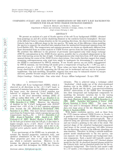
a r X i v :0712.3538v 1 [a s t r o -p h ] 20 D e c 2007Draft version February 2,2008Preprint typeset using L A T E X style emulateapj v.10/09/06COMPARING SUZAKU AND XMM-NEWTON OBSERVATIONS OF THE SOFT X-RAY BACKGROUND:EVIDENCE FOR SOLAR WIND CHARGE EXCHANGE EMISSIONDavid B.Henley and Robin L.SheltonDepartment of Physics and Astronomy,University of Georgia,Athens,GA 30602Draft version February 2,2008ABSTRACTWe present an analysis of a pair of Suzaku spectra of the soft X-ray background (SXRB),obtained from pointings on and oﬀa nearby shadowing ﬁlament in the southern Galactic hemisphere.Because of the diﬀerent Galactic column densities in the two pointing directions,the observed emission from the Galactic halo has a diﬀerent shape in the two spectra.We make use of this diﬀerence when modeling the spectra to separate the absorbed halo emission from the unabsorbed foreground emission from the Local Bubble (LB).The temperatures and emission measures we obtain are signiﬁcantly diﬀerent from those determined from an earlier analysis of XMM-Newton spectra from the same pointing directions.We attribute this diﬀerence to the presence of previously unrecognized solar wind charge exchange (SWCX)contamination in the XMM-Newton spectra,possibly due to a localized enhancement in the solar wind moving across the line of sight.Contemporaneous solar wind data from ACE show nothing unusual during the course of the XMM-Newton observations.Our results therefore suggest that simply examining contemporaneous solar wind data might be inadequate for determining if a spectrum of the SXRB is contaminated by SWCX emission.If our Suzaku spectra are not badly contaminatedby SWCX emission,our best-ﬁtting LB model gives a temperature of log(T LB /K)=5.98+0.03−0.04and a pressure of p LB /k =13,100–16,100cm −3K.These values are lower than those obtained from other recent observations of the LB,suggesting the LB may not be isothermal and may not be in pressure equilibrium.Our halo modeling,meanwhile,suggests that neon may be enhanced relative to oxygen and iron,possibly because oxygen and iron are partly in dust.Subject headings:Galaxy:halo—Sun:solar wind—X-rays:diﬀuse background—X-rays:ISM1.INTRODUCTIONThe diﬀuse soft X-ray background (SXRB),which is observed in all directions in the ∼0.1–2keV band,is composed of emission from several diﬀerent components.For many years,the observed 1/4-keV emission was believed to originate from the Local Bubble (LB),a cavity in the local interstellar medium (ISM)of ∼100pc radius ﬁlled with ∼106K gas (Sanders et al.1977;Cox &Reynolds 1987;McCammon &Sanders 1990;Snowden et al.1990).However,the discovery of shadows in the 1/4-keV background with ROSAT showed that ∼50%of the 1/4keV emission originates from beyond the LB (Burrows &Mendenhall 1991;Snowden et al.1991).This more distant emission origi-nates from the Galactic halo,which contains hot gas with temperatures log(T halo /K)∼6.0–6.5(Snowden et al.1998;Kuntz &Snowden 2000;Smith et al.2007;Galeazzi et al.2007;Henley,Shelton,&Kuntz 2007).As the halo gas is hotter than the LB gas,it also emits at higher energies,up to ∼1keV.Above ∼1keV the X-ray background is extragalactic in origin,and is due to un-resolved active galactic nuclei (AGN;Mushotzky et al.2000).X-ray spectroscopy of the SXRB can,in principle,de-termine the thermal properties,ionization state,and chemical abundances of the hot gas in the Galaxy.These properties give clues to the origin of the hot gas,which is currently uncertain.However,to de-termine the physical properties of the hot Galactic gas,one must ﬁrst decompose the SXRB into its con-Electronic address:dbh@stituents.This is achieved using a technique called “shadowing”,which makes use of the above-mentioned shadows cast in the SXRB by cool clouds of gas be-tween the Earth and the halo.Low-spectral-resolution ROSAT observations of the SXRB were decomposed into their foreground and background components by modeling the intensity variation due to the varying absorption column density on and around shadow-ing clouds (Burrows &Mendenhall 1991;Snowden et al.1991,2000;Snowden,McCammon,&Verter 1993;Kuntz,Snowden,&Verter 1997).The same tech-nique was used to decompose ROSAT All-Sky Survey data over large areas of the sky (Snowden et al.1998;Kuntz &Snowden 2000).With higher resolution spectra,such as those from the CCD cameras onboard XMM-Newton or Suzaku ,it is possible to decompose the SXRB into its foreground and background components spectroscopically.This is achieved using one spectrum toward a shadowing cloud,and one toward a pointing to the side of the cloud.The spectral shape of the absorbed background component (and hence of the overall spectrum)will diﬀer between the two directions,because of the diﬀerent absorbing col-umn densities.Therefore,by ﬁtting a suitable multicom-ponent model simultaneously to the two spectra,one can separate out the foreground and background emis-sion components.Such a model will typically consist of an unabsorbed single-temperature (1T )thermal plasma model for the LB,an absorbed thermal plasma model for the Galactic halo,and an absorbed power-law for the ex-tragalactic background.The Galactic halo model could be a 1T model,a two-temperature (2T )model,or a dif-2HENLEY AND SHELTONferential emission measure (DEM)model (Galeazzi et al.2007;Henley et al.2007;S.J.Lei et al.,in preparation).Recent work has shown that there is an additional complication,as X-ray emission can originate within the solar system,via solar wind charge exchange (SWCX;Cox 1998;Cravens 2000).In this process,highly ion-ized species in the solar wind interact with neutral atoms within the solar system.An electron transfers from a neutral atom into an excited energy level of a solar wind ion,which then decays radiatively,emitting an X-ray photon.The neutral atoms may be in the outer reaches of the Earth’s atmosphere (giving rise to geo-coronal emission),or they may be in interstellar ma-terial ﬂowing through the solar system (giving rise to heliospheric emission).It has been estimated that the heliospheric emission may contribute up to ∼50%of the observed soft X-ray ﬂux (Cravens 2000).The geocoro-nal emission is typically an order of magnitude fainter,but during solar wind enhancements it can be of similar brightness to the heliospheric emission (Wargelin et al.2004).SWCX line emission has been observed with Chandra ,XMM-Newton ,and Suzaku (Wargelin et al.2004;Snowden,Collier,&Kuntz 2004;Fujimoto et al.2007).As the SWCX emission is time varying,it cannot easily be modeled out of a spectrum of the SXRB.If SWCX contamination is not taken into account,analyses of SXRB spectra will yield incorrect results for the LB and halo gas.This paper contains a demonstra-tion of this fact.Henley et al.(2007)analyzed a pair of XMM-Newton spectra of the SXRB using the pre-viously described shadowing technique.One spectrum was from a direction toward a nearby shadowing ﬁlament in the southern Galactic hemisphere (d =230±30pc;Penprase et al.1998),while the other was from a direc-tion ∼2◦away.The ﬁlament and the shadow it casts in the 1/4-keV background are shown in Figure 1.Contem-poraneous solar wind data from the Advanced Composi-tion Explorer (ACE )showed that the solar wind was steady during the XMM-Newton observations,without any ﬂares or spikes.The proton ﬂux was slightly lower than average,and the oxygen ion ratios were fairly typ-ical.These observations led Henley et al.(2007)to con-clude that their spectra were unlikely to be severely con-taminated by SWCX ing a 2T halo model,they obtained a LB temperature of log(T LB /K)=6.06and halo temperatures of log(T halo /K)=5.93and 6.43.The LB temperature and the hotter halo temperature are in good agreement with other recent measurements of the SXRB using XMM-Newton and Suzaku (Galeazzi et al.2007;Smith et al.2007),and with analysis of the ROSAT All-Sky Survey (Kuntz &Snowden 2000).We have obtained spectra of the SXRB from the same directions as Henley et al.’s (2007)XMM-Newton spectra with the X-ray Imaging Spectrometer (XIS;Koyama et al.2007)onboard the Suzaku X-ray obser-vatory (Mitsuda et al.2007).The XIS is an excellent tool for studying the SXRB,due to its low non-X-ray background and good spectral resolution.Our Suzaku pointing directions are shown in Figure 1.We analyze our Suzaku spectra using the same shadowing technique used by Henley et al.(2007).We ﬁnd that there is poor agreement between the results of our Suzaku analysis and the results of the XMM-Newton analysis in Henley et al.(2007).We attribute this discrepancy to previously un-Fig. 1.—The shadowing ﬁlament used for our observations,shown in Galactic coordinates.Grayscale :ROSAT All-Sky Sur-vey R1+R2intensity (Snowden et al.1997).Contours :IRAS 100-micron intensity (Schlegel et al.1998).Yellow squares :Our Suzaku pointing directions.recognized SWCX contamination in the XMM-Newton spectra,which means that SWCX contamination can oc-cur at times when the solar wind ﬂux measured by ACE is low and does not show ﬂares.This paper is organized as follows.The Suzaku obser-vations and data reduction are described in §2.The anal-ysis of the spectra using multicomponent spectral models is described in §3.The discrepancy between the Suzaku results and the XMM-Newton results is discussed in §4.This discrepancy is due to the presence of an additional emission component in the XMM-Newton spectra,which we also describe in §4.In §5we measure the total intensi-ties of the oxygen lines in our Suzaku and XMM-Newton spectra.We concentrate on these lines because they are the brightest in our spectra,and are a major component of the 3/4-keV SXRB (McCammon et al.2002).In §6we present a simple model for estimating the intensity of the oxygen lines due to SWCX,which we compare with our observations.We discuss our results in §7,and con-clude with a summary in §8.Throughout this paper we quote 1σerrors.2.OBSERVATIONS AND DATA REDUCTIONBoth of our observations were carried out in early 2006March.The details of the observations are shown in Ta-ble 1.In the following,we just analyze data from the back-illuminated XIS1chip,as it is more sensitive at lower energies than the three front-illuminated chips.Our data were initially processed at NASA Goddard Space Flight Center (GSFC)using processing version 1.2.2.3.We have carried out further processing and ﬁl-tering,using HEAsoft 1v6.1.2and CIAO 2v3.4.We ﬁrst combined the data taken in the 3×3and 5×5observa-tion modes.We then selected events with grades 0,2,3,4,and 6,and cleaned the data using the standard data selection criteria given in the Suzaku Data Reduc-tion Guide 3.We excluded the times that Suzaku passed through the South Atlantic Anomaly (SAA),and also times up to 436s after passage through the SAA.We also excluded times when Suzaku ’s line of sight was el-evated less than 10◦above the Earth’s limb and/or was1/lheasoft 2/ciao3/docs/suzaku/analysis/abc/abc.htmlOBSERVING CHARGE EXCHANGE WITH SUZAKU AND XMM-NEWTON3TABLE1Details of Our Suzaku ObservationsObservation l b Start time End time Usable exposureID(deg)(deg)(UT)(UT)(ks)Oﬀﬁlament501001010278.71−47.072006-03-0116:56:012006-03-0222:29:1455.6Onﬁlament501002010278.65−45.302006-03-0320:52:002006-03-0608:01:1969.0less than20◦from the bright-Earth terminator.Finally,we excluded times when the cut-oﬀrigidity(COR)wasless than8GV.This is a stricter criterion than that inthe Data Reduction Guide,which recommends exclud-ing times with COR<6GV.However,the higher CORthreshold helps reduce the particle background,and forobservations of the SXRB one desires as low a particlebackground as possible.The COR threshold that weuse has been used for other Suzaku observations of theSXRB(Fujimoto et al.2007;Smith et al.2007).Finally,we binned the2.5–8.5keV data into256-s time bins,andused the CIAO script analyzepublic4HENLEY AND SHELTON34:00.03:33:00.032:00.031:00.015:00.020:00.025:00.0-63:30:00.035:00.040:00.0Right ascensionD e c l i n a t i o nOn filament22:00.021:00.03:20:00.019:00.015:00.0-62:20:00.025:00.030:00.035:00.0Right ascensionD e c l i n a t i o nOff filamentFig.2.—Cleaned and smoothed Suzaku XIS1images in the 0.3–5keV band for our on-ﬁlament (left )and oﬀ-ﬁlament (right )observations.The data have been binned up by a factor of 4in the detector’s x and y directions,and then smoothed with a Gaussian whose standard deviation is equal to 1.5times the binned pixel size.The particle background has not been subtracted from the data.The red circles outline the regions that were excluded from the analysis (see text for details).in our ﬁt (Snowden et al.1997).The R1and R2count-rates help constrain the model al lower energies (below ∼0.3keV),while the higher channels overlap in energy with our Suzaku spectra.We extracted the ROSAT spec-tra from 0.5◦radius circles centered on our two Suzaku pointing directions using the HEASARC X-ray Back-ground Tool 8v2.3.The spectral analysis was carried out using XSPEC 9v11.3.2(Arnaud 1996).For the thermal plasma com-ponents,we used the Astrophysical Plasma Emission Code (APEC)v1.3.1(Smith et al.2001)for the Suzaku data and the ROSAT R4–7bands,and the Raymond-Smith code (Raymond &Smith 1977and updates)for the ROSAT R1–3bands.For a given model component (i.e.,the LB or one of the two halo components),the tem-perature and normalization of the ROSAT Raymond-Smith model are tied to those of the corresponding Suzaku APEC model.We chose to use the Raymond-Smith code for the lower-energy ROSAT channels be-cause APEC’s spectral calculations below 0.25keV are inaccurate,due to a lack of data on transitions from L-shell ions of Ne,Mg,Al,Si,S,Ar,and Ca 10.As the upper-limit of the ROSAT R1and R2bands is 0.284keV,and the R3band also includes such low-energy photons (Snowden et al.1997),APEC is not ideal for ﬁtting to these energy bands.For the absorption,we used the XSPEC phabs model,which uses cross-sections from Ba l uci´n ska-Church &McCammon (1992),with an updated He cross-section from Yan,Sadeghpour,&Dalgarno (1998).Following Henley et al.(2007),we used the interstellar chemical abundance table from Wilms,Allen,&McCray (2000).For many astrophysically abundant elements,these abundances are lower than those in the widely used solar abundance table of Anders &Grevesse (1989).However,recently several elements’solar photospheric abundances have been revised downwards (Asplund et al.2005),and are in good agreement with the Wilms et al.(2000)8/cgi-bin/Tools/xraybg/xraybg.pl9/docs/xanadu/xspec/xspec1110/atomdb/issuesOBSERVING CHARGE EXCHANGE WITH SUZAKU AND XMM-NEWTON5-4-2 0 2 40.3135channel energy (keV)(d a t a -m o d e l )/σ0.001 0.010.11c o u n t s s -1k e V-1On filamentLocal Bubble Halo (cold)Halo (hot)ExtragalacticInstrumental lines TotalO V I I O V I I IN e I XM g X I ?A l KS i KA u M -4-2 0 2 40.3135channel energy (keV)(d a t a -m o d e l )/σ0.0010.010.11c o u n t s s -1k e V-1Off filamentLocal Bubble Halo (cold)Halo (hot)ExtragalacticInstrumental lines TotalN V I I ?O V I I O V I I IN e I XA l KS i KA uMFig.3.—Our observed on-ﬁlament (left )and oﬀ-ﬁlament (right )Suzaku spectra,with the best-ﬁtting model obtained by ﬁtting jointly to the Suzaku and ROSAT data (Model 1in Table 7).The gap in the Si K instrumental line is where channels 500–504have been removed from the data (see §2).10100100010-6 c o u n t s s -1 a r c m i n-2-4-2 0 2 4R1R2R3R4R5R6R7ROSAT band(d a t a - m o d e l ) / σFig. 4.—The on-ﬁlament (dashed )and oﬀ-ﬁlament (solid )ROSAT All-Sky Survey spectra,compared with Model 1from Ta-ble 7.For clarity the individual model components have not been plotted.CALDB.This model component attenuated the emis-sion from the LB,halo,and extragalactic background for the Suzaku spectra only.We adjusted the model oxygen abundance to give C /O =6(Koyama et al.2007),and set the abundances of all other elements to zero.The results of this model are given as Model 2in Table 7.Figures 5and 6show this model com-pared with the Suzaku and ROSAT spectra,respec-tively.One can see from Figure 6that the ﬁt to the ROSAT data is greatly improved.The model implies a column density of carbon atoms,N C =(0.28±0.04)×1018cm −2,in addition to the amount of contamina-tion given by the CALDB contamination model,which is N C =3.1×1018cm −2at the center of the XIS1chip(from the CALDB ﬁle aecontami xrtxis08.html6HENLEY AND SHELTON-4-2 0 2 40.3135channel energy (keV)(d a t a -m o d e l )/σ0.0010.010.1c o u n t s s -1k e V-1On filamentLocal Bubble Halo (cold)Halo (hot)ExtragalacticInstrumental lines Total-4-2 0 2 40.3135channel energy (keV)(d a t a -m o d e l )/σ0.0010.010.1c o u n t s s -1k e V-1Off filamentLocal Bubble Halo (cold)Halo (hot)ExtragalacticInstrumental linesTotalFig. 5.—As Figure 3,but with a vphabs component included for the Suzaku spectra to model XIS contamination above that included in the CALDB (Model 2in Table 7;see §3.2for details).10 100100010-6 c o u n t s s -1 a r c m i n-2-4-2 0 2 4R1R2R3R4R5R6R7ROSAT band(d a t a - m o d e l ) / σFig.6.—As Figure 5,but for Model 2from Table 7.In Model 5we ﬁt exactly the same model to the Suzaku data alone.Without the ROSAT data,we cannot con-strain the LB temperature T LB .We therefore ﬁx it at the value determined in Model 2:T LB =105.98K.We also ﬁx N C for the vphabs contamination component at the Model 2value:N C =0.28×1018cm −2.The best-ﬁtting model parameters are in very good agree-ment with those obtained by ﬁtting jointly to the Suzaku and ROSAT spectra (compare Models 2and 5).We can only get consistent results between the Suzaku -ROSAT joint ﬁt and the ﬁt to just the Suzaku data by using a two-temperature model for the halo.However,note that the Model 5LB emission measure is consistent (within its errorbar)with zero.This is not to say that our data imply that there is no LB at all:as noted above,we need a LB component and two halo components to get a good joint ﬁt to the Suzaku and ROSAT data.Instead,the Model 5results imply that our Suzaku data are consis-tent with the LB not producing signiﬁcant emission in the Suzaku band (i.e.,E 0.3keV).Also shown in Table 7are the results of ﬁtting our model (without any LB component)to the on-and oﬀ-ﬁlament Suzaku spectra individually (Models 6and 7,respectively).As has already been noted,the normaliza-tion of the extragalactic background diﬀers signiﬁcantly between the two spectra.However,the plasma model pa-rameters for the individual spectra are in good agreement with each other.These results seem to justify allowing the extragalactic normalization to diﬀer between the two spectra while keeping all other model parameters equal for the two spectra.3.3.Chemical Abundances in the HaloWe investigated the chemical abundances of the X-ray-emissive halo gas by repeating the above-described mod-eling,but allowing the abundances of certain elements in the halo components to vary.In particular we wished to investigate whether or not varying the neon and magne-sium halo abundances improved the ﬁts to the Ne ix and Mg xi features noted above.We also allowed the abun-dance of iron to vary,as iron is an important contributor of halo line emission to the Suzaku band.For this investigation we just ﬁt to the Suzaku data,ﬁxing the LB temperature at log(T LB /K)=5.98,and ﬁxing the carbon column density of the vphabs contam-ination component at N C =0.28×1018cm −2.As we could not accurately determine the level of the contin-uum due to hydrogen,we could not measure absolute abundances.Instead,we estimated the abundances rel-ative to oxygen by holding the oxygen abundance at its Wilms et al.(2000)value,and allowing the abundances of neon,magnesium,and iron to vary.Both halo com-ponents were constrained to have the same abundances.The best-ﬁtting temperatures and emission measures of the various model components are presented as Model 8in Table 7,and the abundances are presented in Table 2.The best-ﬁtting model parameters are not signiﬁcantly aﬀected by allowing certain elements’abun-dances to vary (compare Model 8with Model 5).Iron does not seem to be enhanced or depleted relative to oxy-gen in the halo.Neon and magnesium both appear to be enhanced in the halo relative to oxygen,which is what one would expect from Figures 3and 5,as the modelsOBSERVING CHARGE EXCHANGE WITH SUZAKU AND XMM-NEWTON7 TABLE2Halo AbundancesElement AbundanceO1(ﬁxed)Ne a1.8±0.4Mg a4.6+3.5−2.8Fe1.2+0.4−0.5Note.—Abun-dances are relative tothe Wilms et al.(2000)interstellar abundances:Ne/O=0.178,Mg/O=0.051,Fe/O=0.055.a These enhanced abun-dances may be an arte-fact of SWCX contami-nation;see§7.2.shown in thoseﬁgures underpredict the neon and mag-nesium emission.We discuss these results in§§7.2and§7.5.In§7.2we discuss the possibility that the enhanced neon and mag-nesium emission is in fact due to SWCX contamination of these lines,rather than being due to these elements being enhanced in the halo.On the other hand,in§7.5 we discuss the implications of neon really being enhanced in the halo with respect to oxygen and iron.PARING THE SUZAKU AND XMM-NEWTONSPECTRAFor comparison,Table7also contains the results of the analysis of the XMM-Newton spectra from the same ob-servation directions by Henley et al.(2007).The Model9 results are taken directly from their“standard”model. However,it should be noted that Henley et al.(2007) used APEC to model all of their data,whereas in the analysis described above we used the Raymond-Smith code to model the ROSAT R1–3bands.We have therefore reanalyzed the XMM-Newton+ROSAT spec-tra,this time using the Raymond-Smith code to model the ROSAT R1–3bands,and using APEC to model the ROSAT R4–7bands and the XMM-Newton spec-tra.This new analysis allows a fairer comparison of our XMM-Newton results with our Suzaku results.The XMM-Newton spectra we analyzed are identical to those used by Henley et al.(2007)–see that paper for details of the data reduction.We added a broken power-law to the model to take into account soft-proton contamination in the XMM-Newton spectra.This broken power-law was not folded through XMM-Newton’s eﬀective area, and was allowed to diﬀer for the on-and oﬀ-ﬁlament datasets(see Henley et al.2007).The presence of this contamination means we cannot independently constrain the normalization of the extragalactic background.We therefore freeze the on-and oﬀ-ﬁlament normalizations at the Suzaku-determined values.The results of this new analysis are presented as Model10in Table7.As can be seen,there is poor agreement between the best-ﬁt parameters of the Suzaku +ROSAT model(Model2)and the XMM-Newton+ ROSAT model(Model10).We believe this discrepancy is due to an extra emission component in the XMM-Newton spectra.In Figure7we plot the diﬀerences between the XMM-Newton spectra and our best-ﬁtting0.10.20.30.40.5data-model(ctss-1keV-1)On filament MOS 1MOS 2 00.10.20.30.40.50.5125channel energy (keV)Off filament MOS 1MOS 2Fig.7.—The excesses in our on-ﬁlament(top)and oﬀ-ﬁlament (bottom)XMM-Newton spectra over our best-ﬁtting model to the Suzaku+ROSAT data(Table7,Model2).The gap in the data between1.4and1.9keV is where two bright instrumental lines have been removed.Suzaku+ROSAT model(Model2from Table7).To our best-ﬁtting Suzaku+ROSAT model we have added a broken power-law to model the soft-proton contami-nation in the XMM-Newton spectra.The parameters of this broken power-law are frozen at the values de-termined from theﬁtting to the XMM-Newton spectra described in the previous paragraph.The on-ﬁlament XMM-Newton spectra show excess line emission at∼0.57 and∼0.65keV,most likely due to O vii and O viii,re-spectively.The features in the oﬀ-ﬁlament spectra are not as clear.However,there appears to be excess O vii emission in the MOS1spectrum,and excess emission at ∼0.7keV(of uncertain origin)and∼0.9keV(proba-bly Ne ix)in the MOS2spectrum.We can estimate the signiﬁcance of the excess emission by calculatingχ2 for the XMM-Newton data compared with the Suzaku +ROSAT model.We concentrate on the excess oxy-gen emission and calculateχ2for the0.5–0.7keV energy range.Weﬁndχ2=106.28for24degrees of freedom for the on-ﬁlament spectra,andχ2=43.03for22degrees of freedom for the oﬀ-ﬁlament spectra.These correspond toχ2probabilities of2.5×10−12and0.0047,respectively, implying that the excesses are signiﬁcant in both sets of spectra at the1%level.We measure the intensities of the extra oxygen emis-sion byﬁttingδ-functions at E=0.570keV and 0.654keV to the excess spectra in Figure7.Weﬁt theseδ-functions simultaneously to the on-and oﬀ-ﬁlament XMM-Newton excess spectra.The intensities of the excess oxygen emission in the XMM-Newton spec-tra over the best-ﬁtting Suzaku+ROSAT model are 3.8±0.5L.U.(O vii)and1.4±0.3L.U.(O viii).We believe that this excess oxygen emission is due to SWCX contamination in our XMM-Newton spectra.As noted in the Introduction,this was not taken into ac-count in the original analysis of the XMM-Newton spec-tra.This is because the solar windﬂux was steady and slightly below average during the XMM-Newton obser-vations,leading Henley et al.(2007)to conclude that SWCX contamination was unlikely to be signiﬁcant.We discuss the SWCX contamination in our spectra further in§6.5.MEASURING THE OXYGEN LINES8HENLEY AND SHELTONAs well as using the above-described method to sep-arate the LB emission from the halo emission,we mea-sured the total intensities of the O vii complex and O viii line at∼0.57and∼0.65keV in each spectrum.These lines are a major component of the SXRB,accounting for the majority of the observed ROSAT R4diﬀuse back-ground that is not due to resolved extragalactic discrete sources(McCammon et al.2002),and are easily the most prominent lines in our Suzaku spectra.To measure the oxygen line intensities,we used a model consisting of an absorbed power-law,an absorbed APEC model whose oxygen abundance is set to zero,and two δ-functions to model the oxygen lines.As in the pre-vious section,the power-law models the extragalactic background,and its photon index was frozen at1.46 (Chen et al.1997).The APEC model,meanwhile,mod-els the line emission from elements other than oxygen, and the thermal continuum emission.The absorbing columns used were the same as those used in the ear-lier Suzaku analysis.As with our earlier analysis,we multiplied the whole model by a vphabs component to model the contamination on the optical blockingﬁlter which is in addition to that included in the CALDB con-tamination model(see§3.2).Weﬁx the carbon column density of this component at0.28×1018cm−2(Table7, Model2).Weﬁt this model simultaneously to our on-and oﬀ-ﬁlament spectra.However,all the model param-eters were independent for the two directions,except for the oxygen line energies–these were free parameters in theﬁt,but were constrained to be the same in the on-and oﬀ-ﬁlament spectra.We used essentially the same method to measure the oxygen line intensities in our XMM-Newton spectra.However,we did not use a vphabs contamination model,and,as before,we added a broken power-law to model the soft-proton contami-nation.Table3gives the energies and total observed intensities of the O vii and O viii emission measured from our Suzaku and XMM-Newton spectra.We can use the diﬀerence in the absorbing column for the on-and oﬀ-ﬁlament directions to decompose the ob-served line intensities into foreground(LB+SWCX)and background(halo)intensities.If I fg and I halo are the in-trinsic foreground and halo line intensities,respectively, then the observed on-ﬁlament intensity I on is given byI on=I fg+e−τon I halo,(1) whereτon is the on-ﬁlament optical depth at the energy of the line.There is a similar expression for the observed oﬀ-ﬁlament intensity I oﬀ,involving the oﬀ-ﬁlament op-tical depthτoﬀ.These expressions can be rearranged to giveI fg=eτon I on−eτoff I oﬀe−τon−e−τoff.(3) For the purposes of this decomposition,we use the Ba l uci´n ska-Church&McCammon(1992)cross-sections (with an updated He cross-section;Yan et al.1998)with the Wilms et al.(2000)interstellar abundances.We use the cross-sections at the measured energies of the lines. For the Suzaku measurements,the cross-sections we use are7.17×10−22cm2for O vii(E=0.564keV)and 4.66×10−22cm2for O viii(E=0.658keV).For the XMM-Newton O vii emission we use a cross-section of 7.03×10−22cm2(E=0.568keV).We cannot decom-pose the XMM-Newton O viii emission because the on-ﬁlament O viii line is brighter than the oﬀ-ﬁlament line. This gives rise to a negative halo intensity,which is un-physical.The results of this decomposition are presented in Ta-ble4.Note that the foreground oxygen intensities mea-sured from the Suzaku spectra are consistent with zero. This is consistent with our earlierﬁnding that the Suzaku spectra are consistent with there being no local emis-sion in the Suzaku band(see§3.2).The diﬀerence be-tween the foreground O vii intensities measured from our XMM-Newton and Suzaku spectra is5.1±3.1L.U.. This is consistent with the O vii intensity measured from the excess XMM-Newton emission over the best-ﬁtting Suzaku+ROSAT model(3.8±0.5L.U.;see§4).The halo O vii intensities measured from our XMM-Newton and Suzaku spectra are consistent with each other.This is as expected,as we would not expect the halo intensity to signiﬁcantly change in∼4years.6.MODELING THE SOLAR WIND CHARGE EXCHANGEEMISSIONIn§§4and5we presented evidence that our XMM-Newton spectra contain an extra emission component,in addition to the components needed to explain the Suzaku spectra.In particular,the O vii and O viii emission are enhanced in the XMM-Newton spectra.We attribute this extra component to SWCX emission,as it seems unlikely to be due to a change in the Local Bubble or halo emission.This extra component helps explain why our XMM-Newton and Suzaku analyses give such diﬀerent results in Table7.Previous observations of SWCX have found that in-creases in the SWCX emission are associated with en-hancements in the solar wind,as measured by ACE. These enhancements consist of an increase in the pro-tonﬂux,and may also include a shift in the ionization balance to higher ionization stages(Snowden et al.2004; Fujimoto et al.2007).In§6.1,we present a simple model for heliospheric and geocoronal SWCX emission,and use contemporaneous solar wind data from the ACE and WIND satellites to determine whether or not the ob-served enhancement of the oxygen lines in the XMM-Newton spectra is due to diﬀerences in the solar wind between our two sets of observations.In addition to the variability associated with solar wind enhancements,the heliospheric SWCX intensity is also expected to vary during the solar cycle,due to the dif-ferent states of the solar wind at solar maximum and solar minimum(Koutroumpa et al.2006).As our two sets of observations were taken∼4years apart,at diﬀer-ent points in the solar cycle,in§6.2we examine whether the SWCX intensity variation during the solar cycle can explain our observations.6.1.A Simple Model for Heliospheric and GeocoronalSWCX Emission6.1.1.The BasicsA SWCX line from a X+n ion of element X results from a charge exchange interaction between a X+(n+1) ion in the solar wind and a neutral atom.The intensity of that line therefore depends on the density of X+(n+1)。

双钙钛矿Ba2LuNbO6∶Tb3+闪烁体多模式X_射线探测

第 44 卷第 9 期2023年 9 月Vol.44 No.9Sept., 2023发光学报CHINESE JOURNAL OF LUMINESCENCE双钙钛矿Ba2LuNbO6∶Tb3+闪烁体多模式X射线探测岳杨1，郭龙超1，刘昊哲2，卜卫芳1，徐旭辉3，谢俊奎4，仇广宇4，王婷2*，余雪1*（1. 成都大学机械工程学院，四川成都　610106；　2.成都理工大学材料与化学化工学院，四川成都　610059；3. 昆明理工大学材料科学与工程学院，云南省新材料制备与加工重点实验室，云南昆明　650093；4. 交通运输部南海航海保障中心北海航标处，广西北海　536000）摘要：采用高温固相法制备了双钙钛矿结构的Ba2LuNbO6∶x Tb3+（x = 0.01，0.02，0.05，0.10，0.20）闪烁体材料，并系统地研究了其晶体结构、形貌和X射线激发的光学性能。

研究表明，在X射线激发下，Ba2LuNbO6∶Tb3+的发射光谱主要由Tb3+的特征发射组成，其中最强发射峰位于545 nm处。

X射线发射（RL）强度随Tb3+浓度的增加逐渐增大，当x = 0.1时发射强度达到最大值。

此外，X射线辐照5 min后的热释光（TL）曲线显示该样品存在位于T1（377 K）和T2（460 K）的两个陷阱。

其陷阱深度分别为0.754 eV和0.920 eV，这表明该材料具有潜在的X射线信息存储性能。

因此，我们可通过加热或者980 nm激光二极管激发，有效诱导读出存储在深陷阱中的载流子，实现高亮度光激励发光（PSL）和热刺激发光（TSL）。

基于此，由Ba2LuNbO6∶Tb3+与聚二甲基硅氧烷（PDMS）所制备的柔性闪烁体薄膜，在低X射线剂量辐照下表现出优异的X射线成像分辨率（12.5 lp/mm）以及延时成像特性。

以上结果表明，所制备的Ba2LuNbO6∶0.1Tb3+在X射线探测和X射线信息存储方面具有潜在的应用前景。

HBL天体中X射线和γ射线辐射研究

HBL天体中X射线和γ射线辐射研究李斯;李丙郎;王雪品;钟微;刘文广【摘要】We study the correlation coefficient between X-ray and γ-ray radiation of BL Lac object Mrk 421 using power-law function F γ-ray∝ F c/sX-ray to describe the relationship between them.Our results show that:(1)the radiation mechanism of X-rays and gamma rays can be explained by synchrotron self-Compton(SSC) model for HBL objects.In the word,X-rays are derived from synchrotron radiation,but the inverse Compton scattering originate from the interaction between the soft photons from the synchrotron radiation and the high energetic electrons,and the gamma rays are produced from the process.(2)the energy band of the X ray maybe affect the size of the index c/s.%利用幂律函数关系Fγ-rayY∝ Fc/sX-ray研究了HBL天体Mrk421的X射线和γ射线辐射流量间的相关系数.研究结果表明:(1)对HBL天体而言,X射线和γ射线的辐射机制可以用均匀自康普顿(SSC)模型来解释,即X射线源于同步辐射,同步辐射过程中产生的软光子和高能电子之间发生逆康普顿散射,产生了γ射线;(2)X射线能段范围会影响到幂律关系式中指数c/s的大小.【期刊名称】《云南师范大学学报（自然科学版）》【年(卷),期】2017(037)004【总页数】9页(P1-9)【关键词】星系;BL Lac天体;辐射机制;非热;方法;相关【作者】李斯;李丙郎;王雪品;钟微;刘文广【作者单位】云南师范大学物理与电子信息学院,云南省高校高能天体物理重点实验室,云南昆明650500;云南师范大学物理与电子信息学院,云南省高校高能天体物理重点实验室,云南昆明650500;云南师范大学物理与电子信息学院,云南省高校高能天体物理重点实验室,云南昆明650500;云南师范大学物理与电子信息学院,云南省高校高能天体物理重点实验室,云南昆明650500;云南师范大学物理与电子信息学院,云南省高校高能天体物理重点实验室,云南昆明650500【正文语种】中文【中图分类】P157.6BL Lac天体多波段能谱分布具有明显的双峰结构，低能峰位于光学波段到软X射线波段，而高能峰位于GeV到TeV区域[1].均匀同步自康普顿(SSC)模型能够较好地解释BL Lac天体的多波段能谱分布，在该模型中，低能峰由喷流内极端相对论性电子的同步辐射产生，而高能峰则由来自同一相对论性电子与同步辐射产生的软光子之间的逆康普顿散射(IC)产生，因此SSC模型认为产生X射线的电子与产生γ射线的电子是同源的.BL Lac天体根据低能峰(同步峰)的位置不同而分为低能峰BL Lac天体(Low-energy Peak BL Lacs,LBL)和高能峰BL Lac天体(High-energy Peak BL Lacs,HBL)，LBL的同步峰主要位于光学波段，而HBL的同步峰主要位于紫外到X射线波段，因而研究HBL天体X射线波段和γ射线波段之间的相关性对于研究该类天体的辐射机制和物理过程有重要的意义.X射线和γ射线能段的观测[2-4]为两者流量同时性变化之间的相关性提供了直接的证据.1998年Mrk 421耀发活动的观测证明了X射线和γ射线之间存在紧密的相关性[5]，证明了高能辐射的光子源于X射线耀发活动中产生的同步辐射软光子.Katarzyński等人[6]详细讨论了HBL天体Mrk 501的X射线辐射变化和TeV γ射线辐射变化之间的相关性，并且给出了一个简单的幂律函数来描述两者之间存在的关系.本文将采用他们对Mrk 501天体的研究思路，对Mrk 421天体X射线辐射变化和γ射线辐射变化之间的相关性进行详细的分析和讨论.均匀同步自康普顿(SSC)模型[6]常被作为HBL天体中X射线辐射和γ射线辐射的一种可能解释.Dermer等人[7-11]的研究工作表明SSC模型对全波段能谱分布(SED)中的X射线和γ射线的辐射机制能够给出较合理且简单的阐释.我们的目的是确定SSC模型是否可以解释光变观测到的具体特征.2.1 均匀同步自康普顿(SSC)模型均匀同步自康普顿(SSC)模型假设存在一个球形区域，且该区域无论处于膨胀状态还是压缩状态，它都是均匀分布的.为了简化物理模型、建立起描述该区域变化的数学表达式，只考虑该区域可能发生的四个基本物理过程：1)该球形区域体积的增加或减少；2)磁场强度的增强或减弱；3)粒子数密度的变化；4)粒子的加速或冷却.为了研究该区域内每个过程对辐射的影响，需要对每一个物理过程进行数学描述. 假设球形区域的半径为R，磁场强度为B.R和B随时间变化，这种变化可以用一个简单的幂律函数来表示：在(1)和(2)式中t0是初始时间, R0是初始区域半径, B0是初始磁场强度，指数re 和m都是自由参量.在初始时刻t0时，区域内电子能量分布可以用一个截断幂律函数来描述是电子洛伦兹因子(相当于电子的能量)，描述的是截断的初始位置，n1是截断前的电子谱指数，n2是截断后的电子谱指数.在模型中我们假设X射线辐射和TeV γ射线辐射的主要成分均由电子能量为γbrk附近的电子产生.电子能谱的演化由下式的最小值决定其中的两个函数的具体表示如下：(5)和(6)式中，K1和K2指的是截断前后粒子数密度的变化，3rd是粒子数密度的增加或减少，粒子加速或冷却由指数ra(n1-1)或ra(n2-1)描述.如果假设的绝热膨胀或绝热压缩的区域内的粒子数密度是一个恒定的常数，那么参数re、ra和rd应该是相等的[12-13].为了分别研究上述过程的影响，需要给出详细的参数结果.电子的同步辐射系数由文献[14]确定，即(7)式中α=.因此，需要定义两个同步辐射系数，即表示低能电子辐射系数，即γ<γbrk；js2表示高能电子辐射系数，即γ>γbrk.忽略电子自吸收过程，因此可以估算出来自球形源的同步辐射强度，即可以求出同步辐射流量变化为(12)和(13)式中，s1是低能电子产生的同步辐射，s2是高能电子产生的同步辐射.以上两个流量之间的主要区别是辐射过程和磁场强度不同.2.2 逆康普顿散射IC自康普顿辐射又被称为逆康普顿散射(Inverse Compton scattering,简称IC). Tavecchio等人[15]用一个截断幂律谱详细研究了SSC辐射过程中的电子能谱.在他们的方法中，逆康普顿散射(IC)谱可以分为四个基本成分.而对于HBL天体，其中只有两个起主导作用的成分能产生自康普顿辐射，即：低能电子(K1,N1)和来自于同步辐射谱的第一部分(Is1,Fs1)共同作用而产生的F1,c,由高能电子(K2,N2)和来自于同步辐射谱的第一部分(Is1,Fs1)共同作用而产生的F2,c.因此，给出逆康普顿散射(IC)过程的主要辐射系数如下：通过类比同步辐射的推导过程，可以求出逆康普顿散射(IC)辐射强度为由此可估算出逆康普顿散射(IC)的流量值：其中c1描述的是在Thomson限制下的逆康普顿散射(IC)散射演化，c2描述的是在Klein-Nishina限制下的逆康普顿散射(IC)散射演化.为了研究HBL天体中X射线和γ射线之间的相关性，所选取的光变曲线必须满足以下条件[6]：1)X射线和γ射线的数据在同一时期内获得；2)两条光变曲线所选取的数据点的样本率相同，即在两条光变曲线上所选取的数据点的个数一致.在HBL天体中，时间变化的尺度非常短，可获得的数据点就比较多，因此光变曲线上的数据点也应该是比较密集的；3)额外的同时性能谱观测提供能谱演化的基本信息，例如，确定同步辐射产生的X射线Fs低于或者高于νFs(ν)峰.在实际的研究工作中，很难找到同时满足以上的所有条件的观测结果，仅在特殊情况下，X射线和γ射线的活动相关性可以被详细地研究和分析.图1展示了在2010年2月观测到的Mrk 421的光变活动.光变曲线分别是由Swift-XRT(0.5-2 keV)、RXTE-ASM(1.5-12 keV)、RXTE-PCA(2-20 keV)、Swift-BAT(15-50 keV)、Fermi-LAT(0.2-300 GeV)和HAGAR(>250 GeV)观测到的.其中X射线波段的光变曲线由Swift-XRT(0.5-2 keV)、RXTE-ASM(1.5-12 keV)、RXTE-PCA(2-20 keV)和Swift-BAT(15-50 keV)观测给出，γ射线波段的光变曲线由Fermi-LAT(0.2-300 GeV)和HAGAR(>250 GeV)观测给出.为了研究两者之间的相关性，需要对不同设备观测到的数据进行两两组合(如表1).观测数据在时间上是随机分布的，为了研究X射线波段和γ射线波段之间的相关性，需要对两个波段观测到的光变曲线进行比较，即选取在同一时段内两个波段同时性或者准同时性数据.但只按照这种方法进行，可能会出现如下情况：光变曲线上虽然有多个数据点，但是满足同时性或者准同时性的数据点相对较少.为了解决这一问题，可以在光变曲线中插入一个同时性的数据点，但注意这样做需要满足光变曲线有相似的采样，采样应该等于或者小于源的光变时间尺度特性变化.某些情况下光变曲线上的观测数据点之间存在着时间偏移，但由于这些数据点均为一天内的基本观测平均值，因此，采用插值法依然可以得到有效的结果.对(12)和(13)式进行对数处理，有对(17)、(18)式进行对数处理，得根据(19)、(20)、(21)、(22)式，得到关系式由(23)式可得在(24)式中，Fs(t)是同步辐射流量，其主要来源于SED图中同步辐射峰附近光子流量，即X射线流量，即FX-ray(t)≡Fs(t),Fc(t)是逆康普顿(IC)散射流量，其主要来源于SED图中IC峰附近光子流量，即γ射线流量，即有Fγ-ray(t)≡Fc(t).所以3.3 数据处理结果根据(23)、(24)、(25)式，对图1中Mrk 421天体光变曲线给出的X射线和γ射线辐射流量进行一元线性回归分析，分析结果如图2和表2所示.根据(23)式，在表2中自变量x表示logFs(t),因变量y表示logFc(t),线性关系的表达式为y=kx+b,其中k=c/s,b-er 是截距的误差范围的绝对值，k-er是斜率的误差范围的绝对值，N是数据点的个数，r为线性相关系数，p为置信度，SD为回归方程的标准偏差.由于k=c/s,根据(24)、(25)式，又可以得到如表3所示的结果.通过分析表2和表3中数据，可以得到以下结果：(1)图2(a)统计的logFXRT和logFLAT间呈现出显著的相关性，其相关系数为r=0.881 13,置信度P=0.020 35；图2(b)统计的logFASM和logFLAT之间也存在着显著的相关性，它的相关系数为r=0.767 62,置信度P=0.015 73；同样地，图2(c)、图2(d)分别统计的logFPCA和logFLAT、logFBAT和logFLAT的相关性也是特别显著的，其中图2(c)的相关系数为r=0.835 71,置信度P=0.019 19，图2(d)的相关系数为r=0.876 88,置信度P=0.004 25.(2)图2(e)、(f)、(g)、(h)中的统计结果分别表明logFXRT和logFHAG、logFASM和logFHAG、logFPCA和logFHAG、logFBAT和logFHAG之间呈现的相关性较弱，因为它们的相关系数r均小于0.5.(3) 当使用Swift-XRT(0.5-2 keV)和Fermi-LAT(0.2-300 GeV)观测时，得到的关系是用RXTE-ASM(1.5-12 keV) 和Fermi-LAT(0.2-300 GeV)观测时，得到的关系是用RXTE-PCA(2-20 keV) 和Fermi-LAT(0.2-300 GeV)观测时，得到的关系是用Swift-BAT(15-50 keV)和Fermi-LAT(0.2-300 GeV)观测时，得到的关系是用Swift-XRT(0.5-2 keV)、RXTE-ASM(1.5-12 keV)、RXTE-PCA(2-20 keV)、Swift-BAT(15-50 keV)探测到的X射线波段的辐射流量与用Fermi-LAT(0.2-300 GeV)观测到的γ射线波段的辐射流量之间存在着显著的相关性.这表明， HBL天体X射线和γ射线的辐射可以用均匀同步自康普顿(SSC)过程来描述，即X射线光子源于同步辐射，GeVγ光子产生于同源电子的逆康普顿散射.用Swift-XRT(0.5-2 keV)、RXTE-ASM(1.5-12 keV)、RXTE-PCA(2-20 keV)、Swift-BAT(15-50 keV)探测到的X射线波段的辐射流量与用HAGAR(E>250 GeV)观测到的γ射线波段的辐射流量之间没有相关性.对此做出如下解释：一般认为HAGAR探测到的γ射线的能量范围E>250 GeV，在这个能量范围以上产生的γ射线为次级γ射线，关于次级γ射线的产生，一种可能的解释是耀变体加速产生的高能宇宙线质子与河外背景光(EBL)光子、宇宙微波背景光(CMB)光子相互作用(pγ相互作用)产生了次级γ射线[17-19]，或者高能光子之间作用产生的正负电子对可能通过逆康普顿散射过程散射微波背景光子，从而产生次级γ射线.如果采用简单的幂律公式来表示X射线和γ射线之间的关系，结合表3中的数据，X射线和γ射线的关系谱指数c/s≤1.Katarzyński等人[6]根据RXTE-PCA观测到的X射线辐射的光变曲线和用HEGRA观测到的TeV γ射线辐射的光变曲线，研究了两者的辐射流量之间的相关性，得到的结果是这个结果与我们的一致.但是我们研究的RXTE-PCA和Fermi-LAT 分别探测到的两条光变曲线的变化比Katarzyński等人用RXTE-PCA和HEGRA观测到的光变曲线的变化更好.根据表3给出的结果，发现X射线能段范围会影响到谱指数c/s的大小，即X射线能段范围不同，谱指数c/s也会不同.这个结论与Katarzyński等人[6]在研究Mrk 501天体时给出的结论是类似的，即相关性斜率可能依赖于谱带宽度.【相关文献】[1] URRY C M.BL Lac Objects and Blazars:Past,Present,and Future[J].ASP Conference series,1999,159:3-19.[2] BUCKLEY J H,AKERLOF C W,BILLER S,et al.Gamma-ray variability of the BL Lacertae object Markarian 421[J].The Astrophysical Journal Letters,1996,472(1):L9.[3] CATANESE M,BRADBURY S M,BRESLIN A C,et al.Multiwavelength observations of a flare from Markarian 501[J].The Astrophysical Journal Letters,1997,487(2):L143.[4] 李斯, 王艳芳, 龙光波,等. 费米耀变体多波段辐射流量相关性研究[J].云南师范大学学报：自然科学版,2015,35(6):1-7.[5] MARASCHI L,FOSSATI G,TAVECCHIO F,et al.Simultaneous X-Ray and TEV observations of a rapid flare from Markarian 421[J].The Astrophysical Journal Letters,1999,526(2):L81.[6] KATARZY SKI K, GHISELLINI G, TAVECCHIO F, et al. Correlation between the TeV and X-ray emission in high-energy peaked BL Lac objects[J].Astronomy &Astrophysics,2005,433(2):479-496.[7] DERMER,CHARLES D,SCHLICKEISER,et al.Model for the High-Energy Emission from Blazars[J]. Astrophysical Journal,1993,416(2):458-484.[8] BEDNAREK W,PROTHEROE R J.Testing the homogeneous synchrotron self Compton model for gamma ray production in Mrk 421[J].Monthly Notices of the Royal Astronomical Society,1997,292(3):646-650.[9] MASTICHIADIS A,KIRK J G.Variability in the synchrotron self-Compton model of blazar emission[J].Astronomy & Astrophysics,1997,320(1):19-25.[10]PIAN E,VACANTI G,TAGLIAFERRI G,et al.BeppoSAX Observations of Unprecedented Synchrotron Activity in the BL Lac Object Mkn 501[J].AstrophysicalJournal,1998,492(1):L17-L20.[11]KATARZY SKI K,SOL H,KUS A.The multifrequency emission of Mrk 501-From radio to TeV gamma-rays[J].Astronomy & Astrophysics,2001,367(3):809-825.[12]KARDASHEV N S.Nonstationarity of Spectra of Young Sources of Nonthermal Radio Emission[J].Soviet Astronomy,1962,6(12):317-327.[13]LONGAIR M S.Book-Review-High Energy Astrophysics-V.1-Particles Photons and TheirDetection-ED.2[J].Science,1992,257(5071):822-823.[14]RYBICKI G B,LIGHTMAN A P.Radiative processes in astrophysics[J].Weinheim:Wiley-VcH Verlag GmbH&Co.KGaA,2007.[15]TAVECCHIO F,MARASCHI L,GHISELLINI G.Constraints on the Physical Parameters of TeV Blazars[J].Astrophysical Journal,1998,509(2):608-619.[16]SHUKLA A,CHITNIS V R,VISHWANATH P R,et al.Multiwavelength study of the TeV blazar Mrk 421 during a giant flare[J].Astronomy & Astrophysics,2012,541(3):1053-1060.[17]ESSEY W,&KUSENKO A. A new interpretation of the gamma-ray observations of distant active galactic nuclei[J].Astropart. Phys.,2010,33(1):81-85.[18]ESSEY W,KALASHEV O E,KUSENKO A,et al.Secondary Photons and Neutrinos from Cosmic Rays Produced by Distant Blazars[J].Phys. Rev. Lett.,2010,104(14):141102.[19]ZHENG Y G,&KANG T.Evidence for secondary emission as the origin of hard spectra in TeV blazars[J].ApJ,2013,764(2):113-118.。

低红移SDSS类星体辐射效率的估计

低红移SDSS类星体辐射效率的估计吴淑梅;张福鹏;陆烨;陆由俊【摘要】研究了低红移SDSS类星体(0.025＜z＜0.5)的辐射效率.首先利用类星体中心黑洞的质量估计,通过薄盘吸积模型估计了每一个类星体的吸积率.其次根据光学波段的观测光度,利用经验的类星体全波段模板谱估计了每个类星体的热光度.最后由估计的吸积率和热光度得到了每个类星体的辐射效率.发现低红移SDSS类星体的辐射效率与黑洞质量强相关,并满足ε∝M.0.63.这一结果与Davis和Laor(2011)对PG类星体样本得到的结果一致.进一步讨论由于辐射效率估计中各种假设可能引入的偏差及其对ε与M.关系的可能影响.【期刊名称】《天文研究与技术－国家天文台台刊》【年(卷),期】2014(011)002【总页数】7页(P95-101)【关键词】吸积盘;辐射效率;黑洞;吸积率;自旋【作者】吴淑梅;张福鹏;陆烨;陆由俊【作者单位】中国科学院国家天文台,北京100012;中国科学院国家天文台,北京100012;中国科学院国家天文台,北京100012;中国科学院国家天文台,北京100012【正文语种】中文【中图分类】P142.9CN53－1189/P ISSN1672－7673一般认为大质量黑洞的物质吸积是活动星系核和类星体的能量来源。

类星体的光学紫外辐射近似地可用几何薄光学厚的标准薄吸积盘描述[1]。

有关大质量黑洞和类星体的观测统计表明其中心黑洞是通过类星体阶段的物质吸积获得绝大部分质量[2－3]。

大质量黑洞的形成演化和类星体的吸积历史密切相关。

例如，如果吸积过程是长期的薄盘吸积，其中心黑洞的自旋会快速演化至接近于1的一个平衡态值；但若吸积过程为具有随机角动量的多个短时标吸积，吸积阶段测量其黑洞自旋很可能接近于0[4－5]。

在标准薄盘模型中，类星体的光谱发射主要取决于几个基本的参数，即黑洞的质量M•、自旋a、质量吸积率acc以及吸积盘相对于观测视线的倾角i等。

黑洞的准正模式(quasinormal modes)

Quasi-Normal Modes of Stars and Black HolesKostas D.KokkotasDepartment of Physics,Aristotle University of Thessaloniki,Thessaloniki54006,Greece.kokkotas@astro.auth.grhttp://www.astro.auth.gr/˜kokkotasandBernd G.SchmidtMax Planck Institute for Gravitational Physics,Albert Einstein Institute,D-14476Golm,Germany.bernd@aei-potsdam.mpg.dePublished16September1999/Articles/Volume2/1999-2kokkotasLiving Reviews in RelativityPublished by the Max Planck Institute for Gravitational PhysicsAlbert Einstein Institute,GermanyAbstractPerturbations of stars and black holes have been one of the main topics of relativistic astrophysics for the last few decades.They are of partic-ular importance today,because of their relevance to gravitational waveastronomy.In this review we present the theory of quasi-normal modes ofcompact objects from both the mathematical and astrophysical points ofview.The discussion includes perturbations of black holes(Schwarzschild,Reissner-Nordstr¨o m,Kerr and Kerr-Newman)and relativistic stars(non-rotating and slowly-rotating).The properties of the various families ofquasi-normal modes are described,and numerical techniques for calculat-ing quasi-normal modes reviewed.The successes,as well as the limits,of perturbation theory are presented,and its role in the emerging era ofnumerical relativity and supercomputers is discussed.c 1999Max-Planck-Gesellschaft and the authors.Further information on copyright is given at /Info/Copyright/.For permission to reproduce the article please contact livrev@aei-potsdam.mpg.de.Article AmendmentsOn author request a Living Reviews article can be amended to include errata and small additions to ensure that the most accurate and up-to-date infor-mation possible is provided.For detailed documentation of amendments, please go to the article’s online version at/Articles/Volume2/1999-2kokkotas/. Owing to the fact that a Living Reviews article can evolve over time,we recommend to cite the article as follows:Kokkotas,K.D.,and Schmidt,B.G.,“Quasi-Normal Modes of Stars and Black Holes”,Living Rev.Relativity,2,(1999),2.[Online Article]:cited on<date>, /Articles/Volume2/1999-2kokkotas/. The date in’cited on<date>’then uniquely identiﬁes the version of the article you are referring to.3Quasi-Normal Modes of Stars and Black HolesContents1Introduction4 2Normal Modes–Quasi-Normal Modes–Resonances7 3Quasi-Normal Modes of Black Holes123.1Schwarzschild Black Holes (12)3.2Kerr Black Holes (17)3.3Stability and Completeness of Quasi-Normal Modes (20)4Quasi-Normal Modes of Relativistic Stars234.1Stellar Pulsations:The Theoretical Minimum (23)4.2Mode Analysis (26)4.2.1Families of Fluid Modes (26)4.2.2Families of Spacetime or w-Modes (30)4.3Stability (31)5Excitation and Detection of QNMs325.1Studies of Black Hole QNM Excitation (33)5.2Studies of Stellar QNM Excitation (34)5.3Detection of the QNM Ringing (37)5.4Parameter Estimation (39)6Numerical Techniques426.1Black Holes (42)6.1.1Evolving the Time Dependent Wave Equation (42)6.1.2Integration of the Time Independent Wave Equation (43)6.1.3WKB Methods (44)6.1.4The Method of Continued Fractions (44)6.2Relativistic Stars (45)7Where Are We Going?487.1Synergism Between Perturbation Theory and Numerical Relativity487.2Second Order Perturbations (48)7.3Mode Calculations (49)7.4The Detectors (49)8Acknowledgments50 9Appendix:Schr¨o dinger Equation Versus Wave Equation51Living Reviews in Relativity(1999-2)K.D.Kokkotas and B.G.Schmidt41IntroductionHelioseismology and asteroseismology are well known terms in classical astro-physics.From the beginning of the century the variability of Cepheids has been used for the accurate measurement of cosmic distances,while the variability of a number of stellar objects(RR Lyrae,Mira)has been associated with stel-lar oscillations.Observations of solar oscillations(with thousands of nonradial modes)have also revealed a wealth of information about the internal structure of the Sun[204].Practically every stellar object oscillates radially or nonradi-ally,and although there is great diﬃculty in observing such oscillations there are already results for various types of stars(O,B,...).All these types of pulsations of normal main sequence stars can be studied via Newtonian theory and they are of no importance for the forthcoming era of gravitational wave astronomy.The gravitational waves emitted by these stars are extremely weak and have very low frequencies(cf.for a discussion of the sun[70],and an im-portant new measurement of the sun’s quadrupole moment and its application in the measurement of the anomalous precession of Mercury’s perihelion[163]). This is not the case when we consider very compact stellar objects i.e.neutron stars and black holes.Their oscillations,produced mainly during the formation phase,can be strong enough to be detected by the gravitational wave detectors (LIGO,VIRGO,GEO600,SPHERE)which are under construction.In the framework of general relativity(GR)quasi-normal modes(QNM) arise,as perturbations(electromagnetic or gravitational)of stellar or black hole spacetimes.Due to the emission of gravitational waves there are no normal mode oscillations but instead the frequencies become“quasi-normal”(complex), with the real part representing the actual frequency of the oscillation and the imaginary part representing the damping.In this review we shall discuss the oscillations of neutron stars and black holes.The natural way to study these oscillations is by considering the linearized Einstein equations.Nevertheless,there has been recent work on nonlinear black hole perturbations[101,102,103,104,100]while,as yet nothing is known for nonlinear stellar oscillations in general relativity.The study of black hole perturbations was initiated by the pioneering work of Regge and Wheeler[173]in the late50s and was continued by Zerilli[212]. The perturbations of relativistic stars in GR wereﬁrst studied in the late60s by Kip Thorne and his collaborators[202,198,199,200].The initial aim of Regge and Wheeler was to study the stability of a black hole to small perturbations and they did not try to connect these perturbations to astrophysics.In con-trast,for the case of relativistic stars,Thorne’s aim was to extend the known properties of Newtonian oscillation theory to general relativity,and to estimate the frequencies and the energy radiated as gravitational waves.QNMs wereﬁrst pointed out by Vishveshwara[207]in calculations of the scattering of gravitational waves by a Schwarzschild black hole,while Press[164] coined the term quasi-normal frequencies.QNM oscillations have been found in perturbation calculations of particles falling into Schwarzschild[73]and Kerr black holes[76,80]and in the collapse of a star to form a black hole[66,67,68]. Living Reviews in Relativity(1999-2)5Quasi-Normal Modes of Stars and Black Holes Numerical investigations of the fully nonlinear equations of general relativity have provided results which agree with the results of perturbation calculations;in particular numerical studies of the head-on collision of two black holes [30,29](cf.Figure 1)and gravitational collapse to a Kerr hole [191].Recently,Price,Pullin and collaborators [170,31,101,28]have pushed forward the agreement between full nonlinear numerical results and results from perturbation theory for the collision of two black holes.This proves the power of the perturbation approach even in highly nonlinear problems while at the same time indicating its limits.In the concluding remarks of their pioneering paper on nonradial oscillations of neutron stars Thorne and Campollataro [202]described it as “just a modest introduction to a story which promises to be long,complicated and fascinating ”.The story has undoubtedly proved to be intriguing,and many authors have contributed to our present understanding of the pulsations of both black holes and neutron stars.Thirty years after these prophetic words by Thorne and Campollataro hundreds of papers have been written in an attempt to understand the stability,the characteristic frequencies and the mechanisms of excitation of these oscillations.Their relevance to the emission of gravitational waves was always the basic underlying reason of each study.An account of all this work will be attempted in the next sections hoping that the interested reader will ﬁnd this review useful both as a guide to the literature and as an inspiration for future work on the open problems of the ﬁeld.020406080100Time (M ADM )-0.3-0.2-0.10.00.10.20.3(l =2) Z e r i l l i F u n c t i o n Numerical solutionQNM fit Figure 1:QNM ringing after the head-on collision of two unequal mass black holes [29].The continuous line corresponds to the full nonlinear numerical calculation while the dotted line is a ﬁt to the fundamental and ﬁrst overtone QNM.In the next section we attempt to give a mathematical deﬁnition of QNMs.Living Reviews in Relativity (1999-2)K.D.Kokkotas and B.G.Schmidt6 The third and fourth section will be devoted to the study of the black hole and stellar QNMs.In theﬁfth section we discuss the excitation and observation of QNMs andﬁnally in the sixth section we will mention the more signiﬁcant numerical techniques used in the study of QNMs.Living Reviews in Relativity(1999-2)7Quasi-Normal Modes of Stars and Black Holes 2Normal Modes–Quasi-Normal Modes–Res-onancesBefore discussing quasi-normal modes it is useful to remember what normal modes are!Compact classical linear oscillating systems such asﬁnite strings,mem-branes,or cavitiesﬁlled with electromagnetic radiation have preferred time harmonic states of motion(ωis real):χn(t,x)=e iωn tχn(x),n=1,2,3...,(1) if dissipation is neglected.(We assumeχto be some complex valuedﬁeld.) There is generally an inﬁnite collection of such periodic solutions,and the“gen-eral solution”can be expressed as a superposition,χ(t,x)=∞n=1a n e iωn tχn(x),(2)of such normal modes.The simplest example is a string of length L which isﬁxed at its ends.All such systems can be described by systems of partial diﬀerential equations of the type(χmay be a vector)∂χ∂t=Aχ,(3)where A is a linear operator acting only on the spatial variables.Because of theﬁniteness of the system the time evolution is only determined if some boundary conditions are prescribed.The search for solutions periodic in time leads to a boundary value problem in the spatial variables.In simple cases it is of the Sturm-Liouville type.The treatment of such boundary value problems for diﬀerential equations played an important role in the development of Hilbert space techniques.A Hilbert space is chosen such that the diﬀerential operator becomes sym-metric.Due to the boundary conditions dictated by the physical problem,A becomes a self-adjoint operator on the appropriate Hilbert space and has a pure point spectrum.The eigenfunctions and eigenvalues determine the periodic solutions(1).The deﬁnition of self-adjointness is rather subtle from a physicist’s point of view since fairly complicated“domain issues”play an essential role.(See[43] where a mathematical exposition for physicists is given.)The wave equation modeling theﬁnite string has solutions of various degrees of diﬀerentiability. To describe all“realistic situations”,clearly C∞functions should be suﬃcient. Sometimes it may,however,also be convenient to consider more general solu-tions.From the mathematical point of view the collection of all smooth functions is not a natural setting to study the wave equation because sequences of solutionsLiving Reviews in Relativity(1999-2)K.D.Kokkotas and B.G.Schmidt8 exist which converge to non-smooth solutions.To establish such powerful state-ments like(2)one has to study the equation on certain subsets of the Hilbert space of square integrable functions.For“nice”equations it usually happens that the eigenfunctions are in fact analytic.They can then be used to gen-erate,for example,all smooth solutions by a pointwise converging series(2). The key point is that we need some mathematical sophistication to obtain the “completeness property”of the eigenfunctions.This picture of“normal modes”changes when we consider“open systems”which can lose energy to inﬁnity.The simplest case are waves on an inﬁnite string.The general solution of this problem isχ(t,x)=A(t−x)+B(t+x)(4) with“arbitrary”functions A and B.Which solutions should we study?Since we have all solutions,this is not a serious question.In more general cases, however,in which the general solution is not known,we have to select a certain class of solutions which we consider as relevant for the physical problem.Let us consider for the following discussion,as an example,a wave equation with a potential on the real line,∂2∂t2χ+ −∂2∂x2+V(x)χ=0.(5)Cauchy dataχ(0,x),∂tχ(0,x)which have two derivatives determine a unique twice diﬀerentiable solution.No boundary condition is needed at inﬁnity to determine the time evolution of the data!This can be established by fairly simple PDE theory[116].There exist solutions for which the support of theﬁelds are spatially compact, or–the other extreme–solutions with inﬁnite total energy for which theﬁelds grow at spatial inﬁnity in a quite arbitrary way!From the point of view of physics smooth solutions with spatially compact support should be the relevant class–who cares what happens near inﬁnity! Again it turns out that mathematically it is more convenient to study all solu-tions ofﬁnite total energy.Then the relevant operator is again self-adjoint,but now its spectrum is purely“continuous”.There are no eigenfunctions which are square integrable.Only“improper eigenfunctions”like plane waves exist.This expresses the fact that weﬁnd a solution of the form(1)for any realωand by forming appropriate superpositions one can construct solutions which are “almost eigenfunctions”.(In the case V(x)≡0these are wave packets formed from plane waves.)These solutions are the analogs of normal modes for inﬁnite systems.Let us now turn to the discussion of“quasi-normal modes”which are concep-tually diﬀerent to normal modes.To deﬁne quasi-normal modes let us consider the wave equation(5)for potentials with V≥0which vanish for|x|>x0.Then in this case all solutions determined by data of compact support are bounded: |χ(t,x)|<C.We can use Laplace transformation techniques to represent such Living Reviews in Relativity(1999-2)9Quasi-Normal Modes of Stars and Black Holes solutions.The Laplace transformˆχ(s,x)(s>0real)of a solutionχ(t,x)isˆχ(s,x)= ∞0e−stχ(t,x)dt,(6) and satisﬁes the ordinary diﬀerential equations2ˆχ−ˆχ +Vˆχ=+sχ(0,x)+∂tχ(0,x),(7) wheres2ˆχ−ˆχ +Vˆχ=0(8) is the homogeneous equation.The boundedness ofχimplies thatˆχis analytic for positive,real s,and has an analytic continuation onto the complex half plane Re(s)>0.Which solutionˆχof this inhomogeneous equation gives the unique solution in spacetime determined by the data?There is no arbitrariness;only one of the Green functions for the inhomogeneous equation is correct!All Green functions can be constructed by the following well known method. Choose any two linearly independent solutions of the homogeneous equation f−(s,x)and f+(s,x),and deﬁneG(s,x,x )=1W(s)f−(s,x )f+(s,x)(x <x),f−(s,x)f+(s,x )(x >x),(9)where W(s)is the Wronskian of f−and f+.If we denote the inhomogeneity of(7)by j,a solution of(7)isˆχ(s,x)= ∞−∞G(s,x,x )j(s,x )dx .(10) We still have to select a unique pair of solutions f−,f+.Here the information that the solution in spacetime is bounded can be used.The deﬁnition of the Laplace transform implies thatˆχis bounded as a function of x.Because the potential V vanishes for|x|>x0,the solutions of the homogeneous equation(8) for|x|>x0aref=e±sx.(11) The following pair of solutionsf+=e−sx for x>x0,f−=e+sx for x<−x0,(12) which is linearly independent for Re(s)>0,gives the unique Green function which deﬁnes a bounded solution for j of compact support.Note that for Re(s)>0the solution f+is exponentially decaying for large x and f−is expo-nentially decaying for small x.For small x however,f+will be a linear com-bination a(s)e−sx+b(s)e sx which will in general grow exponentially.Similar behavior is found for f−.Living Reviews in Relativity(1999-2)K.D.Kokkotas and B.G.Schmidt 10Quasi-Normal mode frequencies s n can be deﬁned as those complex numbers for whichf +(s n ,x )=c (s n )f −(s n ,x ),(13)that is the two functions become linearly dependent,the Wronskian vanishes and the Green function is singular!The corresponding solutions f +(s n ,x )are called quasi eigenfunctions.Are there such numbers s n ?From the boundedness of the solution in space-time we know that the unique Green function must exist for Re (s )>0.Hence f +,f −are linearly independent for those values of s .However,as solutions f +,f −of the homogeneous equation (8)they have a unique continuation to the complex s plane.In [35]it is shown that for positive potentials with compact support there is always a countable number of zeros of the Wronskian with Re (s )<0.What is the mathematical and physical signiﬁcance of the quasi-normal fre-quencies s n and the corresponding quasi-normal functions f +?First of all we should note that because of Re (s )<0the function f +grows exponentially for small and large x !The corresponding spacetime solution e s n t f +(s n ,x )is therefore not a physically relevant solution,unlike the normal modes.If one studies the inverse Laplace transformation and expresses χas a com-plex line integral (a >0),χ(t,x )=12πi +∞−∞e (a +is )t ˆχ(a +is,x )ds,(14)one can deform the path of the complex integration and show that the late time behavior of solutions can be approximated in ﬁnite parts of the space by a ﬁnite sum of the form χ(t,x )∼N n =1a n e (αn +iβn )t f +(s n ,x ).(15)Here we assume that Re (s n +1)<Re (s n )<0,s n =αn +iβn .The approxi-mation ∼means that if we choose x 0,x 1, and t 0then there exists a constant C (t 0,x 0,x 1, )such that χ(t,x )−N n =1a n e (αn +iβn )t f +(s n ,x ) ≤Ce (−|αN +1|+ )t (16)holds for t >t 0,x 0<x <x 1, >0with C (t 0,x 0,x 1, )independent of t .The constants a n depend only on the data [35]!This implies in particular that all solutions deﬁned by data of compact support decay exponentially in time on spatially bounded regions.The generic leading order decay is determined by the quasi-normal mode frequency with the largest real part s 1,i.e.slowest damping.On ﬁnite intervals and for late times the solution is approximated by a ﬁnite sum of quasi eigenfunctions (15).It is presently unclear whether one can strengthen (16)to a statement like (2),a pointwise expansion of the late time solution in terms of quasi-normal Living Reviews in Relativity (1999-2)11Quasi-Normal Modes of Stars and Black Holes modes.For one particular potential(P¨o schl-Teller)this has been shown by Beyer[42].Let us now consider the case where the potential is positive for all x,but decays near inﬁnity as happens for example for the wave equation on the static Schwarzschild spacetime.Data of compact support determine again solutions which are bounded[117].Hence we can proceed as before.Theﬁrst new point concerns the deﬁnitions of f±.It can be shown that the homogeneous equation(8)has for each real positive s a unique solution f+(s,x)such that lim x→∞(e sx f+(s,x))=1holds and correspondingly for f−.These functions are uniquely determined,deﬁne the correct Green function and have analytic continuations onto the complex half plane Re(s)>0.It is however quite complicated to get a good representation of these func-tions.If the point at inﬁnity is not a regular singular point,we do not even get converging series expansions for f±.(This is particularly serious for values of s with negative real part because we expect exponential growth in x).The next new feature is that the analyticity properties of f±in the complex s plane depend on the decay of the potential.To obtain information about analytic continuation,even use of analyticity properties of the potential in x is made!Branch cuts may occur.Nevertheless in a lot of cases an inﬁnite number of quasi-normal mode frequencies exists.The fact that the potential never vanishes may,however,destroy the expo-nential decay in time of the solutions and therefore the essential properties of the quasi-normal modes.This probably happens if the potential decays slower than exponentially.There is,however,the following way out:Suppose you want to study a solution determined by data of compact support from t=0to some largeﬁnite time t=T.Up to this time the solution is–because of domain of dependence properties–completely independent of the potential for suﬃciently large x.Hence we may see an exponential decay of the form(15)in a time range t1<t<T.This is the behavior seen in numerical calculations.The situation is similar in the case ofα-decay in quantum mechanics.A comparison of quasi-normal modes of wave equations and resonances in quantum theory can be found in the appendix,see section9.Living Reviews in Relativity(1999-2)K.D.Kokkotas and B.G.Schmidt123Quasi-Normal Modes of Black HolesOne of the most interesting aspects of gravitational wave detection will be the connection with the existence of black holes[201].Although there are presently several indirect ways of identifying black holes in the universe,gravitational waves emitted by an oscillating black hole will carry a uniqueﬁngerprint which would lead to the direct identiﬁcation of their existence.As we mentioned earlier,gravitational radiation from black hole oscillations exhibits certain characteristic frequencies which are independent of the pro-cesses giving rise to these oscillations.These“quasi-normal”frequencies are directly connected to the parameters of the black hole(mass,charge and angu-lar momentum)and for stellar mass black holes are expected to be inside the bandwidth of the constructed gravitational wave detectors.The perturbations of a Schwarzschild black hole reduce to a simple wave equation which has been studied extensively.The wave equation for the case of a Reissner-Nordstr¨o m black hole is more or less similar to the Schwarzschild case,but for Kerr one has to solve a system of coupled wave equations(one for the radial part and one for the angular part).For this reason the Kerr case has been studied less thoroughly.Finally,in the case of Kerr-Newman black holes we face the problem that the perturbations cannot be separated in their angular and radial parts and thus apart from special cases[124]the problem has not been studied at all.3.1Schwarzschild Black HolesThe study of perturbations of Schwarzschild black holes assumes a small per-turbation hµνon a static spherically symmetric background metricds2=g0µνdxµdxν=−e v(r)dt2+eλ(r)dr2+r2 dθ2+sin2θdφ2 ,(17) with the perturbed metric having the formgµν=g0µν+hµν,(18) which leads to a variation of the Einstein equations i.e.δGµν=4πδTµν.(19) By assuming a decomposition into tensor spherical harmonics for each hµνof the formχ(t,r,θ,φ)= mχ m(r,t)r Y m(θ,φ),(20)the perturbation problem is reduced to a single wave equation,for the func-tionχ m(r,t)(which is a combination of the various components of hµν).It should be pointed out that equation(20)is an expansion for scalar quantities only.From the10independent components of the hµνonly h tt,h tr,and h rr transform as scalars under rotations.The h tθ,h tφ,h rθ,and h rφtransform asLiving Reviews in Relativity(1999-2)13Quasi-Normal Modes of Stars and Black Holes components of two-vectors under rotations and can be expanded in a series of vector spherical harmonics while the components hθθ,hθφ,and hφφtransform as components of a2×2tensor and can be expanded in a series of tensor spher-ical harmonics(see[202,212,152]for details).There are two classes of vector spherical harmonics(polar and axial)which are build out of combinations of the Levi-Civita volume form and the gradient operator acting on the scalar spherical harmonics.The diﬀerence between the two families is their parity. Under the parity operatorπa spherical harmonic with index transforms as (−1) ,the polar class of perturbations transform under parity in the same way, as(−1) ,and the axial perturbations as(−1) +11.Finally,since we are dealing with spherically symmetric spacetimes the solution will be independent of m, thus this subscript can be omitted.The radial component of a perturbation outside the event horizon satisﬁes the following wave equation,∂2∂t χ + −∂2∂r∗+V (r)χ =0,(21)where r∗is the“tortoise”radial coordinate deﬁned byr∗=r+2M log(r/2M−1),(22) and M is the mass of the black hole.For“axial”perturbationsV (r)= 1−2M r ( +1)r+2σMr(23)is the eﬀective potential or(as it is known in the literature)Regge-Wheeler potential[173],which is a single potential barrier with a peak around r=3M, which is the location of the unstable photon orbit.The form(23)is true even if we consider scalar or electromagnetic testﬁelds as perturbations.The parameter σtakes the values1for scalar perturbations,0for electromagnetic perturbations, and−3for gravitational perturbations and can be expressed asσ=1−s2,where s=0,1,2is the spin of the perturbingﬁeld.For“polar”perturbations the eﬀective potential was derived by Zerilli[212]and has the form V (r)= 1−2M r 2n2(n+1)r3+6n2Mr2+18nM2r+18M3r3(nr+3M)2,(24)1In the literature the polar perturbations are also called even-parity because they are characterized by their behavior under parity operations as discussed earlier,and in the same way the axial perturbations are called odd-parity.We will stick to the polar/axial terminology since there is a confusion with the deﬁnition of the parity operation,the reason is that to most people,the words“even”and“odd”imply that a mode transforms underπas(−1)2n or(−1)2n+1respectively(for n some integer).However only the polar modes with even have even parity and only axial modes with even have odd parity.If is odd,then polar modes have odd parity and axial modes have even parity.Another terminology is to call the polar perturbations spheroidal and the axial ones toroidal.This deﬁnition is coming from the study of stellar pulsations in Newtonian theory and represents the type ofﬂuid motions that each type of perturbation induces.Since we are dealing both with stars and black holes we will stick to the polar/axial terminology.Living Reviews in Relativity(1999-2)K.D.Kokkotas and B.G.Schmidt14where2n=( −1)( +2).(25) Chandrasekhar[54]has shown that one can transform the equation(21)for “axial”modes to the corresponding one for“polar”modes via a transforma-tion involving diﬀerential operations.It can also be shown that both forms are connected to the Bardeen-Press[38]perturbation equation derived via the Newman-Penrose formalism.The potential V (r∗)decays exponentially near the horizon,r∗→−∞,and as r−2∗for r∗→+∞.From the form of equation(21)it is evident that the study of black hole perturbations will follow the footsteps of the theory outlined in section2.Kay and Wald[117]have shown that solutions with data of compact sup-port are bounded.Hence we know that the time independent Green function G(s,r∗,r ∗)is analytic for Re(s)>0.The essential diﬃculty is now to obtain the solutions f±(cf.equation(10))of the equations2ˆχ−ˆχ +Vˆχ=0,(26) (prime denotes diﬀerentiation with respect to r∗)which satisfy for real,positives:f+∼e−sr∗for r∗→∞,f−∼e+r∗x for r∗→−∞.(27) To determine the quasi-normal modes we need the analytic continuations of these functions.As the horizon(r∗→∞)is a regular singular point of(26),a representation of f−(r∗,s)as a converging series exists.For M=12it reads:f−(r,s)=(r−1)s∞n=0a n(s)(r−1)n.(28)The series converges for all complex s and|r−1|<1[162].(The analytic extension of f−is investigated in[115].)The result is that f−has an extension to the complex s plane with poles only at negative real integers.The representation of f+is more complicated:Because inﬁnity is a singular point no power series expansion like(28)exists.A representation coming from the iteration of the deﬁning integral equation is given by Jensen and Candelas[115],see also[159]. It turns out that the continuation of f+has a branch cut Re(s)≤0due to the decay r−2for large r[115].The most extensive mathematical investigation of quasi-normal modes of the Schwarzschild solution is contained in the paper by Bachelot and Motet-Bachelot[35].Here the existence of an inﬁnite number of quasi-normal modes is demonstrated.Truncating the potential(23)to make it of compact support leads to the estimate(16).The decay of solutions in time is not exponential because of the weak decay of the potential for large r.At late times,the quasi-normal oscillations are swamped by the radiative tail[166,167].This tail radiation is of interest in its Living Reviews in Relativity(1999-2)。

CMB Observations and the Production of Chemical Elements at the End of the Dark Ages

Key words. cosmology: cosmic microwave background – cosmology: theory – intergalactic medium – atomic processes – abundances
1. Introduction
High precision observations of CMB anisotropies are giving us unique information about the angular distribution of CMB ﬂuctuations, as well as their spectral dependence in a very broad frequency range. HFI and LFI detectors of PLANCK1 spacecraft will provide unprecedented sensitivity in 9 broad band (∆ν/ν ∼ 20 − 30%) channels, uniformly distributed in the spectral region of the CMB where contribution of diﬀerent foregrounds are expected to be at a minimum. CMBpol and other proposed missions are expected to reach noise levels 20 - 100 times lower than that of PLANCK HFI with technology already available (Church 2002). The WMAP2 satellite was designed to provide measurements of the CMB temperature anisotropies in the whole sky with an average sensitivity of 35µK per 0.3◦ × 0.3◦ pixel at the end of the mission (Bennett et al. 2002, Page et al. 2002). Once such sensitivity limit is reached, the WMAP data will be the ﬁrst real-life test

超大质量双黑洞系统中的吸积盘Formationand

系统喷流方向不变。现有的观测表明，FRII射电星系中的吸积~盘10是8 y标r 准
的而FRI射电星系中的吸积盘则很可能是非标准的
•观测：大约 7%的射电源属于X-形态源 [Leahy & Parma 92] •理论：喷流等离子体遗迹可探测时间大约一千万年，7%的探测概率意味着低亮度的FRII射电星系寿命大约一亿年。这和测得的AGN寿命一致
rL
1
1 m
2/3
rs
m=
if 104
The whole inner region is destroyed by waves
if 104 and H/r<0.1
Opens a gap in the accretion disk The outer boundary of the gap:
evolution merging
Galaxy + galaxy
Normal galaxy
星系与活动星系的大统一模型（？）
gas: starbursts galaxy Evolution Short-lived AGNs
Martini 2004 106 yr tQ a few 108 yr
1.3、Gravitational Wave Astrophysics:
•观测：喷流遗迹与寄住星系盘垂直 •理论：在吸积盘与超大质量双黑洞发生相互作用前，吸积盘因角动量守恒而与星系盘共面，因而产生的喷流与吸积盘和星系盘垂直
•观测：活动的喷流随机取向 •理论：新喷流方向垂直于双黑洞轨道面，而星系并合形成的超大质量双黑洞相对于星系盘取向随机
Random distribution of jet orientations (Liu, Zhang, Wu, 2005, in preparation)

UBVI CCD photometry of two old open clusters NGC 1798 and NGC 2192

a r X i v :a s t r o -p h /9901140v 1 12 J a n 1999Mon.Not.R.Astron.Soc.000,1–8(1998)Printed 1February 2008(MN L A T E X style ﬁle v1.4)UBV I CCD photometry of two old open clusters NGC 1798and NGC 2192Hong Soo Park and Myung Gyoon Lee ⋆Department of Astronomy,Seoul National University,Seoul 151-742,KoreaAccepted 1998??.Received 1998??;in original form 1998July ??ABSTRACT We present UBV I CCD photometry of two open clusters NGC 1798and NGC 2192which were little studied before.Color-magnitude diagrams of these clusters show several features typical for old open clusters:a well-deﬁned main-sequence,a red giant clump,and a small number of red giants.The main sequence of NGC 1798shows a distinct gap at V ≈16.2mag.From the surface number density distribution we have measured the size of the clusters,obtaining 8′.3(=10.2pc)for NGC 1798and 7′.3(=7.5pc)for NGC 2192.Then we have determined the reddening,metallicity,and distance of these clusters using the color-color diagrams and color-magnitude diagrams:E (B −V )=0.51±0.04,[Fe/H]=−0.47±0.15dex and (m −M )0=13.1±0.2(d =4.2±0.3kpc)for NGC 1798,and E (B −V )=0.20±0.03,[Fe/H]=−0.31±0.15dex and (m −M )0=12.7±0.2(d =3.5±0.3kpc)for NGC 2192.The ages of these clusters have been estimated using the morphological age indicators and the isochrone ﬁtting with the Padova isochrones:1.4±0.2Gyrs for NGC 1798and 1.1±0.1Gyrs for NGC 2192.The luminosity functions of the main sequence stars in these clusters are found to be similar to other old open clusters.The metallicity and distance of these clusters are consistent with the relation between the metallicity and galactocentric distance of other old open clusters.Key words:Hertzsprung–Russell (HR)diagram –open clusters and associations:general –open clusters and associations:individual:NGC 1798,NGC 2192–stars:luminosity function.1INTRODUCTIONOld open clusters provide us with an important informationfor understanding the early evolution of the Galactic disk.There are about 70known old open clusters with age >1Gyrs (Friel 1995).These clusters are faint in general so thatthere were few studies about these clusters until recently.With the advent of CCD camera in astronomy,the numberof studies on these clusters has been increasing.However,there are still a signiﬁcant number of old open clusters forwhich basic parameters are not well known.For example,metallicity is not yet known for about 30clusters amongthem.Recently Phelps et al.(1994)and Janes &Phelps (1994)presented an extensive CCD photometric survey of potentialold open clusters,the results of which were used in the studyon the development of the Galactic disk by Janes &Phelps(1994).In the sample of the clusters studied by Phelps et al.⋆corresponding author,E-mail:mglee@astrog.snu.ac.krthere are several clusters for which only the non-calibrated photometry is available.We have chosen two clusters among them,NGC 1798and NGC 2192,to study the characteristics of these clus-ters using UBV I CCD photometry.These clusters are lo-cated in the direction of anti-galactic centre.To date there is published only one photometric study of these clusters,which was given by Phelps et al.(1994)who presented non-calibrated BV CCD photometry of these clusters.From the instrumental color-magnitude diagrams of these clus-ters Phelps et al.estimated the ages of these clusters using the morphological age indicators,obtaining the values of 1.5Gyrs for NGC 1798and 1.1Gyrs for NGC 2192.However,no other properties of these clusters are yet known.In this paper we present a study of NGC 1798and NGC 2192based on UBV I CCD photometry.We have es-timated the basic parameters of these clusters:size,red-dening,metallicity,distance,and age.Also we have derived the luminosity function of the main sequence stars in these clusters.Section 2describes the observations and data re-duction.Sections 3and 4present the analysis for NGC 1798c 1998RAS2Hong Soo Park and Myung Gyoon Leeand NGC2192,respectively.Section5discusses the results. Finally Section6summarizes the primary results.2OBSER V ATIONS AND DATA REDUCTION 2.1ObservationsUBV I CCD images of NGC1798and NGC2192were obtained using the Photometrics512CCD camera at the Sobaeksan Observatory61cm telescope in Korea for several observing runs between1996November and1997October. We have used also BV CCD images of the central region of NGC1798obtained by Chul Hee Kim using the Tek1024 CCD camera at the Vainu Bappu Observatory2.3m tele-scope in India on March4,1998.The observing log is given in Table1.The original CCD images wereﬂattened after bias sub-traction and several exposures for eachﬁlter were combined into a single image for further reduction.The sizes of the ﬁeld in a CCD image are4′.3×4′.3for the PM512CCD im-age,and10′.6×10′.6for the Tek1024CCD image.The gain and readout noise are,respectively,9electrons/ADU and 10.4electrons for the PM512CCD,and9electrons/ADU and10.4electrons for the Tek1024CCD.Figs.1and2illustrate grey scale maps of the V CCD images of NGC1798and NGC2192made by mosaicing the images of the observed regions.It is seen from theseﬁgures that NGC1798is a relatively rich open cluster,while NGC 2192is a relatively poor open cluster.2.2Data ReductionInstrumental magnitudes of the stars in the CCD images were obtained using the digital stellar photometry reduction program IRAF⋆/DAOPHOT(Stetson1987,Davis1994). The resulting instrumental magnitudes were transformed onto the standard system using the standard stars from Lan-dolt(1992)and the M67stars in Montgomery et al.(1993) observed on the same photometric nights.The transforma-tion equations areV=v+a V(b−v)+k V X+Z V,(B−V)=a BV(b−v)+k BV X+Z BV,(U−B)=a UB(u−b)+k UB X+Z UB,and(V−I)=a V I(v−i)+k V I X+Z V I,where the lower case symbols represent instrumental mag-nitudes derived from the CCD images and the upper case symbols represent the standard system values.X is the air-mass at the midpoint of the observations.The results of the transformation are summarized in Table2.The data ob-tained on non-photometric nights were calibrated using the photometric data for the overlapped region.The total number of the measured stars is1,416for NGC1798and409for NGC2192.Tables3and4list the⋆IRAF is distributed by the National Optical Astronomy Ob-servatories,which are operated by the Association of Universities for Research in Astronomy,Inc.under contract with the National Science Foundation.photometry of the bright stars in the C-regions of NGC1798 and NGC2192,respectively.The X and Y coordinates listed in Table3and4are given in units of CCD pixel(=0′′.50). The X and Y values are increasing toward north and west, respectively.We have divided the entire region of theﬁelds into sev-eral regions,as shown in Figs.1and2,for the analysis of the data.The C-region represents the central region of the cluster,and the F-regions(F,Fb,Fir,and Fi regions)rep-resent the controlﬁeld regions,and the N-region represents the intermediate region between the central region and the ﬁeld region.The radius of the C-region is300pixel for NGC 1798and NGC2192.The ratio of the areas of the C-region, N-region,Fb-region,and(Fi+Fir)-regions for NGC1798is 1:1.50:1.00:1.07,and the ratio of the areas of the C-region, N-region,and F-region for NGC2192is1:1.26:0.98.3ANALYSIS FOR NGC17983.1The Size of the ClusterWe have investigated the structure of NGC1798using star-counts.The centre of the cluster is estimated to be at the po-sition of(X=710pixel,Y=1110pixel),using the centroid method.Fig.3illustrates the projected surface number den-sity proﬁle derived from counting stars with V<19.5mag in the entire CCDﬁeld.The magnitude cutoﬀfor starcounts was set so that the counts should be free of any photometric incompleteness problem.Fig.3shows that most of the stars in NGC1798are concentrated within the radius of250pixel (=125′′),and that the outskirts of the cluster extend out to about500pixel(=250′′)from the center.The number density changes little with radius beyond500pixel,show-ing that the outer region of the observedﬁeld can be used as a controlﬁeld.Therefore we have estimated the approxi-mate size of NGC1798for which the cluster blends in with theﬁeld to be about500′′in diameter,which corresponds to a linear size of10.2pc for the distance of NGC1798as determined below.3.2Color-Magnitude DiagramsFigs.4and5show the V−(B−V)and V−(V−I)color-magnitude diagrams(CMDs)of the measured stars in the observed regions in NGC1798.Theseﬁgures show that the C-region consists mostly of the members of NGC1798with some contamination of theﬁeld stars,while the F-regions consist mostly of theﬁeld stars.The N-region is intermediate between the C-region and the F-region.The distinguishable features seen in the color-magnitude diagrams of the C-region are:(a)There is a well-deﬁned main sequence the top of which is located at V≈16 mag;(b)There is seen a distinct gap at V≈16.2mag in the main sequence,which is often seen in other old open clusters (e.g.M67);(c)There is a poorly deﬁned red giant branch and these is seen some excess of stars around(B−V)=1.3 and V=15.6mag on this giant branch,which is remarked by the small box in theﬁgures.This may be a random excess of stars.However,the positions of the stars in the CMDs are consistent with the positions of known red giant clump in other old open clusters.Therefore most of these stars arec 1998RAS,MNRAS000,1–8UBV I CCD photometry of two old open clusters NGC1798and NGC21923probably red giant clump stars;and(d)There are a small number of stars along the locus of the red giant branch. 3.3Reddening and MetallicityNGC1798is located close to the galactic plane in the anti-galactic centre direction(b=4◦.85and l=160◦.76)so that it is expected that the reddening toward this cluster is signiﬁcant.We have estimated the reddening for NGC1798 using two methods as follows.First we have used the mean color of the red giant clump.Janes&Phelps(1994)estimated the mean color and magnitude of the red giant clump in old open clusters to be (B−V)RGC=0.87±0.02and M V,RGC=0.59±0.09,when the diﬀerence between the red giant clump and the main sequence turn-oﬀof the clusters,δV,is smaller than one. The mean color of the red giant clump in the C-region is estimated to be(B−V)RGC=1.34±0.01((V−I)RGC= 1.47±0.01,and(U−B)RGC=1.62±0.04),and the cor-responding mean magnitude is V RGC=15.57±0.05.δV is estimated to be0.8±0.2,which is the same value derived by Phelps et al.(1994).From these data we have derived a value of the reddening,E(B−V)=0.47±0.02.Secondly we have used the color-color diagram to es-timate the reddening and the metallicity simultaneously. We haveﬁtted the mean colors of the stars in the C-region with the color-color relation used in the Padova isochrones (Bertelli et al.1994).This process requires iteration,because we need to know the age of the cluster as well as the red-dening and metallicity.We have iterated this process until all three parameters are stabilized.Fig.6illustrates the results ofﬁtting in the(U−B)−(B−V)color-color diagram.It is shown in thisﬁgure that the stars in NGC1798are reasonablyﬁtted by the color-color relation of the isochrones for[Fe/H]=−0.47±0.15 with a reddening value of E(B−V)=0.55±0.05. The error for the metallicity,0.15,was estimated by com-paring isochrones with diﬀerent metallicities.As a reference the mean locus of the giants for solar abundance given by Schmidt-Kaler(1982)is also plotted in Fig.6.Finally we derive a mean value of the two estimates for the reddening, E(B−V)=0.51±0.04.3.4DistanceWe have estimated the distance to NGC1798using two methods as follows.First we have used the mean magnitude of the red giant clump.We have derived a value of the ap-parent distance modulus(m−M)V=14.98±0.10from the values for the mean magnitudes of the red giant clump stars described above.Secondly we have used the the zero-age main sequence (ZAMS)ﬁtting,following the method described in Vanden-Berg&Poll(1989).VandenBerg&Poll(1989)presented the semi-empirical ZAMS as a function of the metallicity[Fe/H] and the helium abundance Y:V=M V(B−V)+δM V(Y)+δM V([Fe/H])whereδM V(Y)=2.6(Y−0.27)andδM V([Fe/H])=−[Fe/H](1.444+0.362[Fe/H]).Before the ZAMSﬁtting,we subtracted statistically the contribution due to theﬁeld stars in the CMDs of the C-region using the CMDs of the Fb-region for BV photometry and the CMDs of the Fi+Fir region for V I photometry. The size of the bin used for the subtraction is∆V=0.25 and∆(B−V)=0.1.The resulting CMDs are displayed in Fig.7.We used the metallicity of[Fe/H]=–0.47as derived above and adopted Y=0.28which is the mean value for old open clusters(Gratton1982).Using this method we have obtained a value of the apparent distance modulus(m−M)V=14.5±0.2.Finally we calculate a mean value of the two estimates,(m−M)V=14.7±0.2.Adopting the extinction law of A V=3.2E(B−V),we derive a value of the intrinsic distance modulus(m−M)0=13.1±0.2.This corresponds to a distance of d=4.2±0.3kpc.3.5AgeWe have estimated the age of NGC1798using two methods as follows.First we have used the morphological age index (MAI)as described in Phelps et al.(1994).Phelps et al. (1994)and Janes&Phelps(1994)presented the MAI–δV relation,MAI[Gyrs]=0.73×10(0.256δV+0.0662δV2).From the value ofδV derived above,0.8±0.2mag,we obtain a value for the age,MAI=1.3±0.2Gyrs.Secondly we have estimated the age of the cluster us-ing the theoretical isochrones given by the Padova group (Bertelli et al.1994).Fitting the isochrones for[Fe/H]=–0.47to the CMDs of NGC1798,as shown in Fig.8,we estimate the age to be1.4±0.2Gyrs.Both results agree very well.3.6Luminosity FunctionWe have derived the V luminosity functions of the main sequence stars in NGC1798,which are displayed in Fig.9.The Fb-region was used for subtraction of theﬁeld star contribution from the C-region and the magnitude bin size used is0.5mag.This controlﬁeld may not be far enough from the cluster to derive theﬁeld star contribution.If so,we might have oversubtracted theﬁeld contribution,obtaining ﬂatter luminosity functions than true luminosity functions. However,the fraction of the cluster members in thisﬁeld must be,if any,very low,because the surface number density of this region is almost constant with the radius as shown in Fig.3.The luminosity function of the C-region in Fig. 9(a)increases rapidly up to V≈16.5mag,and stays almost ﬂat for V>16.5mag.The luminosity functions of the N-region and the(R+Fir)-region are steeper than that of the C-region.A remarkable drop is seen at V=16.2mag(M V= 1.5mag)in the luminosity function of the C-region based on smaller bin size of0.2mag in Fig.9(b).This corresponds to the main sequence gap described above.4ANALYSIS FOR NGC21924.1The Size of the ClusterWe have investigated the structure of NGC2192using star-counts.We could not use the centroid method to estimatec 1998RAS,MNRAS000,1–84Hong Soo Park and Myung Gyoon Leethe centre of this cluster,because this cluster is too sparse. So we have used eye-estimate to determine the centre of the cluster to be at the position of(X=465pixel,Y=930 pixel).Fig.10illustrates the projected surface number den-sity proﬁle derived from counting stars with V<18mag in the entire CCDﬁeld.The magnitude cutoﬀfor starcounts was set so that the counts should be free of any photomet-ric incompleteness problem.Fig.10shows that most of the stars in NGC2192are concentrated within the radius of200 pixel(=100′′),and that the outskirts of the cluster extend out to about440pixel(=220′′)from the centre.Therefore the approximate size of NGC2192is estimated to be about 440′′in diameter,which corresponds to a linear size of7.5pc for the distance of NGC2192as determined below.4.2Color-Magnitude DiagramsFigs.11and12show the V−(B−V)and V−(V−I)color-magnitude diagrams of the measured stars in the observed regions in NGC2192.The distinguishable features seen in the color-magnitude diagrams of the C-region are:(a)There is a well-deﬁned main sequence the top of which is located at V≈14mag;(b)There are a group of red giant clump stars at(B−V)=1.1and V=14.2mag,which are remarked by the small box in theﬁgures;and(c)There are a small number of stars along the locus of the red giant branch. 4.3Reddening and MetallicityNGC2192is located11degrees above the galactic plane in the anti-galactic centre direction(b=10◦.64and l= 173◦.41)but higher than NGC1798so that it is expected that the reddening toward this cluster is signiﬁcant but smaller than that of NGC1798.We have estimated the red-dening for NGC2192using two methods as applied for NGC 1798.First we have used the mean color of the red giant clump.The mean color of the red giant clump in the C-region is estimated to be(B−V)RGC=1.08±0.01((V−I)RGC=1.07±0.01,and(U−B)RGC=0.61±0.02),and the corresponding mean magnitude is V RGC=14.20±0.05.δV is estimated to be0.6±0.2,which is similar to the value derived by Phelps et al.(1994).From these data we have derived a value of the reddening,E(B−V)=0.19±0.03.Secondly we have used the color-color diagram to es-timate the reddening and the metallicity simultaneously. We haveﬁtted the mean colors of the stars in the C-region with the color-color relation used in the Padova isochrones (Bertelli et al.1994).Fig.13illustrates the results ofﬁt-ting in the(U−B)−(B−V)color-color diagram.It is shown in thisﬁgure that the stars in NGC2192are rea-sonablyﬁtted by the color-color relation of the isochrones for[Fe/H]=−0.31±0.15dex with a reddening value of E(B−V)=0.21±0.01.The error for the metallicity,0.15, was estimated by comparing isochrones with diﬀerent metal-licities.As a reference the mean locus of the giant for solar abundance given by Schmidt-Kaler is also plotted in Fig.13. Finally we derive a mean value of the two estimates for the reddening,E(B−V)=0.20±0.03.4.4DistanceWe have estimated the distance to NGC2192using two methods as for NGC1798.First we have used the mean magnitude of the red giant clump.We have derived a value of the apparent distance modulus(m−M)V=13.61±0.10 from the values for the mean magnitudes of the red giant clump stars described previously.Secondly we have used the ZAMSﬁtting.Before the ZAMSﬁtting,we subtracted statistically the contribution due to theﬁeld stars in the CMDs of the C-region using the CMDs of the F-region.The size of the bin used for the subtraction is∆V=0.25and∆(B−V)=0.1.The resulting CMDs are displayed in Fig.14.We used the metallicity of[Fe/H]=–0.31as derived before and adopted Y=ing this method we have obtaineda value of the apparent distance modulus(m−M)V=13.1±0.2.Finally we calculate a mean value of the two estimates,(m−M)V=13.3±0.2.Adopting the extinction law of A V=3.2E(B−V),we derive a value of the intrinsic distance modulus(m−M)0=12.7±0.2.This corresponds to a distance of d=3.5±0.3kpc.4.5AgeWe have estimated the age of NGC2192using two methods as follows.First we have used the morphological age index. From the value ofδV derived above,0.6±0.2mag,we obtain a value for the age,MAI=1.1±0.2Gyrs.Secondly we have estimated the age of the cluster using the theoretical isochrones given by the Padova group(Bertelli et al.1994). Fitting the isochrones for[Fe/H]=–0.31to the CMDs of NGC2192,as shown in Fig.15,we estimate the age to be 1.1±0.1Gyrs.Both results agree very well.4.6Luminosity FunctionWe have derived the V luminosity functions of the main sequence stars in NGC2192,which are displayed in Fig.16.The F-region was used for subtraction of theﬁeld star contribution from the C-region.The luminosity function of the C-region in Fig.16(a)increases rapidly up to V≈14 mag,and stays almostﬂat for V>15mag.The luminosity function of the N-region is steeper than that of the C-region. Fig.16(b)displays a comparison of the luminosity functions of NGC1798,NGC2192,and NGC7789which is another old open cluster of similar age(Roger et al.1994).Fig.16(b) shows that the luminosity functions of these clusters are similar in that they are almostﬂat in the faint part.The ﬂattening of the faint part of the luminosity functions of old open clusters has been known since long,and is believed to be due to evaporation of low mass stars(Friel1995).5DISCUSSIONWe have determined the metallicity and distance of NGC 1798and NGC2192in this study.We compare them with those of other old open clusters here.Fig.17illustrates the radial metallicity gradient of the old open clusters com-piled by Friel(1995)and supplemented by the data in Wee&Lee(1996)and Lee(1997).Fig.17shows that thec 1998RAS,MNRAS000,1–8UBV I CCD photometry of two old open clusters NGC1798and NGC21925 mean metallicity decreases as the galactocentric distance in-creases.The positions of NGC1798and NGC2192we haveobtained in this study are consistent with the mean trendof the other old open clusters.The slope we have deter-mined for the entire sample including these two clusters is∆[Fe/H]/R GC=−0.086±0.011dex/kpc,very similar tothat given in Friel(1995),∆[Fe/H]/R GC=−0.091±0.014dex/kpc.There are only four old open clusters located beyondR GC=13kpc in Fig.17.These four clusters follow the meantrend of decreasing outward.However,the number of theclusters is not large enough to decide whether the metallictykeeps decreasing outward or it stops decreasing somewherebeyond R GC=13kpc and stays constant.Further studiesof more old open clusters beyond R GC=13kpc are neededto investigate this point.6SUMMARY AND CONCLUSIONSWe have presented UBV I photometry of old open clustersNGC1798and NGC2192.From the photometric data wehave determined the size,reddening,metallicity,distance,and age of these clusters.The luminosity functions of themain sequence stars in these clusters are similar to those ofthe other old open clusters.The basic properties of theseclusters we have determined in this study are summarizedin Table5.ACKNOWLEDGMENTSProf.Chul Hee Kim is thanked for providing the BV CCDimages of NGC1798.This research is supported in part bythe Korea Science and Engineering Foundation Grant No.95-0702-01-01-3.REFERENCESBertelli,G.,Bressan,A.,Chiosi,C.,Fagotto,F.,&Nasi,E.1994,A&AS,106,275Davis,L.E.,1994,A Reference Guide to the IRAF/DAOPHOTPackageFriel,E.D.1995,ARA&A,33,381Gratton,R.G.,1982,ApJ,257,640Janes,K.,&Phelps,R.L.1994,AJ,108,1773Landolt,A.U.,1992,AJ,104,340Lee,M.G.,1997,113,729Montgomery,K.A.,Marschall,L.A.,&Janes,K.A.1993,AJ,106,181Phelps,R.L.,Janes,K.,&Montgomery,K.A.,1994,AJ,107,1079Roger,C.M.,Paez,E.,Castellani,V.,&Staniero,O.1994,A&A,290,62Schmidt-Kaler,T.1982,in Landolt-Bornstein VI,2b(Berlin:Springer)Stetson,P.B.,1987,PASP,99,191VandenBerg,D.A.,&Poll,H.E.,1989,AJ,98,1451Wee,S.O.,&Lee,M.G.,1996,Jour.Korean Astro.Soc.,29,181This paper has been produced using the Royal AstronomicalSociety/Blackwell Science L A T E X styleﬁle.c 1998RAS,MNRAS000,1–86Hong Soo Park and Myung Gyoon LeeTable2.Transformation coeﬃcients for the standard stars.Date Color a k Z rms n(stars) 96.11.11V0.003–0.101–6.0400.00919(B−V) 1.090–0.155–0.4670.01317(U−B) 1.008–0.154–1.7110.03416 97.02.11V0.028–0.198–6.0500.00934(B−V) 1.150–0.118–0.5930.01035(U−B) 1.079–0.324–1.5750.03226(V−I)0.983–0.1300.3020.00829 97.02.13V–0.007–0.176–6.0050.01034(B−V) 1.160–0.133–0.5880.01334(U−B) 1.079–0.349–1.5260.02320(V−I)0.986–0.0970.2710.01532 97.03.17V-0.019–0.225–6.0680.01548(B−V) 1.221–0.093–0.7810.01844(U−B) 1.008–0.309–1.4580.02735(V−I)0.956–0.1570.3140.02052Table 3.UBV I photometry of the bright stars in the C-regionof NGC1798.ID X[px]Y[px]V(B−V)(U−B)(V−I) 1723.21110.815.8600.7790.3240.9143680.51092.015.380 1.3250.627 1.5254746.01160.315.9050.7410.2200.9545741.81165.514.380 1.4830.880 1.6336684.61030.115.8140.8640.342 1.0427745.31073.315.3760.9200.237 1.0849707.21038.814.777 1.4860.723 1.653 11549.41153.715.305 1.5290.915 1.666 12547.91162.714.846 1.6270.947 1.764 13602.31068.015.325 1.5240.847 1.660 14598.11080.815.776 1.3340.575 1.490 15525.81116.815.510 1.0020.346 1.169 18833.91144.214.976 1.4940.866 1.578 21981.91125.114.711 1.510 1.031 1.440 26835.71098.015.706 1.3180.468 1.407 27656.51022.115.653 1.4160.180 1.571 28659.8955.915.216 1.2160.384 1.385 29656.4976.813.6670.6610.3100.777 30674.2822.512.0330.4450.0500.532 33668.7966.315.687 1.3130.641 1.446 34764.3879.915.460 1.3370.508 1.408 38749.01008.115.359 1.3220.744 1.426 39774.4965.915.545 1.3040.590 1.402 43571.8930.612.875 1.970 1.264 2.252 45512.8908.715.810 1.3480.474 1.485 46642.1949.515.622 1.3290.590 1.477 48732.61211.315.821 1.3530.643 1.492 50678.81210.515.297 1.3680.770 1.501 51742.11244.414.7990.747-0.046 1.216 52673.11250.215.180 1.3060.780 1.457 56728.21183.415.665 1.4050.803 1.545 57614.91229.413.085 2.1770.635 3.581 62563.01338.415.9090.7060.6380.778 65913.91203.013.686 1.2490.851 1.354 67792.71314.215.6010.9750.470 1.275 68932.61268.414.4660.7170.1970.763 70801.11338.715.561 1.3270.785 1.442 72827.61315.513.5260.9670.521 1.161 78444.01094.814.605 1.5790.825 1.723 82684.3822.615.8280.9510.128 1.189 97598.51330.315.580 1.3360.710 1.483Table4.UBV I photometry of the bright stars in the C-region of NGC2192.ID X[px]Y[px]V(B−V)(U−B)(V−I) 4502.4879.614.9830.4320.1140.424 5537.5891.712.9690.9240.4750.930 7535.1931.315.1700.598-0.2010.483 9434.8947.613.6760.570-0.0560.648 10562.3991.914.037 1.0960.612 1.043 11412.9884.814.165 1.0780.608 1.072 12598.4778.715.1840.464-0.0300.477 13595.9930.014.4800.5020.1720.549 14625.8971.814.7430.7200.0890.741 16614.3684.214.3970.7660.1750.758 17463.3689.514.7660.4660.0120.480 18553.3710.715.4920.447-0.1350.428 19591.7723.814.4660.5450.0930.566 21623.0867.712.634 1.1020.713 1.108 22648.0929.015.3380.3940.1150.399 26461.1711.314.162 1.0860.670 1.091 29583.9802.315.0940.600-0.0160.644 32720.4889.515.3260.3700.0710.410 37395.9778.315.2640.3960.0310.379 38405.5778.514.8900.4810.1010.409 40258.21042.915.4310.4240.1200.484 42376.6883.915.1870.4550.1360.470 44180.1908.714.3200.2870.1120.295 47367.1938.314.8970.4030.2520.459 51183.3998.714.202 1.1140.552 1.108 55475.81052.514.6370.3880.1670.465 56389.11055.113.6060.6520.2560.777 58481.41074.114.3470.4500.1150.520 59514.91085.115.0970.4290.1370.517 60478.51089.614.2360.5280.1590.582 61498.51127.914.6090.5090.1350.578 63278.71154.414.372 1.0700.599 1.053 64527.41158.715.4180.4460.2450.510 65343.41167.814.266 1.0120.618 1.035 66362.21169.314.2660.8790.4690.879 74346.91039.814.5810.4520.1240.510 77688.91124.215.4200.3900.2900.400 83678.91079.715.4950.4640.1070.504 84624.21042.813.5010.3850.2170.389 88579.61028.914.8250.4560.1620.530 Table5.Basic properties of NGC1798and NGC2192.Parameter NGC1798NGC2192RA(2000)5h11m40s6h15m11sDEC(2000)47◦40′37′′39◦51′1′′l160◦.76173◦.41b4◦.8510◦.64Age1.4±0.2Gyrs1.1±0.1GyrsE(B−V)0.51±0.040.20±0.04[Fe/H]−0.47±0.15dex−0.31±0.15dex(m−M)013.1±0.212.7±0.2distance4.2±0.3kpc3.5±0.3kpcR GC12.5kpc11.9kpcz355pc646pcdiameter10.2pc(8′.3)7.5pc(7′.3)c 1998RAS,MNRAS000,1–8UBV I CCD photometry of two old open clusters NGC1798and NGC21927 Table1.Observing log for NGC1798and NGC2192.Date Target Filter Seeing Telescope Condition96.11.11NCC1798UBV2′′.3SAO a-61cm Photometric97.01.12NCC1798UBV I2′′.2SAO-61cm Non-photometric97.02.12NCC1798,NGC2192UBV I3′′.3SAO-61cm Photometric97.02.13NCC1798,NGC2192UBV I2′′.5SAO-61cm Non-photometric97.03.17NCC2192UBV I2′′.2SAO-61cm Photometric97.10.21NCC1798BV I2′′.3SAO-61cm Non-photometric97.10.24NCC2192BV I2′′.7SAO-61cm Non-photometric97.03.04NCC1798BV2′′.7VBO b-2.3m Non-photometrica Sobaeksan Astronomical Observatoryb Vainu Bappu Observatoryc 1998RAS,MNRAS000,1–8。

材料分析方法习题

第一章分析下列荧光辐射产生的可能性，为什么？（1）用CuKαX射线激发CuKα荧光辐射；（2）用CuKβX射线激发CuKα荧光辐射；（3）用答：根据经典原子模型，原子内的电子分布在一系列量子化的壳层上，在稳定状态下，每个壳层有一定数量的电子，他们有一定的能量。

最内层能量最低，向外能量依次增加。

根据能量关系，M、K层之间的能量差大于L、K成之间的能量差，K、L层之间的能量差大于M、L层能量差。

由于释放的特征谱线的能量等于壳层间的能量差，所以K?0?8的能量大于Ka的能量，Ka能量大于La的能量。

因此在不考虑能量损失的情况下：CuKa能激发CuKa荧光辐射；（能量相同）CuK?0?8能激发CuKa荧光辐射；（K?0?8>Ka）CuKa能激发CuLa荧光辐射；（Ka>la）什么叫“相干散射”、“非相干散射”、“荧光辐射”、“吸收限”、“俄歇效应”？答：⑴当χ射线通过物质时，物质原子的电子在电磁场的作用下将产生受迫振动，受迫振动产生交变电磁场，其频率与入射线的频率相同，这种由于散射线与入射线的波长和频率一致，位相固定，在相同方向上各散射波符合相干条件，故称为相干散射。

⑵当χ射线经束缚力不大的电子或自由电子散射后，可以得到波长比入射χ射线长的χ射线，且波长随散射方向不同而改变，这种散射现象称为非相干散射。

⑶一个具有足够能量的χ射线光子从原子内部打出一个K电子，当外层电子来填充K空位时，将向外辐射K系χ射线，这种由χ射线光子激发原子所发生的辐射过程，称荧光辐射。

或二次荧光。

⑷指χ射线通过物质时光子的能量大于或等于使物质原子激发的能量，如入射光子的能量必须等于或大于将K电子从无穷远移至K层时所作的功W，称此时的光子波长λ称为K系的吸收限。

⑸当原子中K层的一个电子被打出后，它就处于K激发状态，其能量为E k。

如果一个L层电子来填充这个空位，K电离就变成了L电离，其能由Ek变成El，此时将释Ek-El的能量，可能产生荧光χ射线，也可能给予L层的电子，使其脱离原子产生二次电离。

泛珠综合试试题及答案-solution-14

when the wood was still part of a living tree. (1 point) 假设我们从史前古墓的一块木头得到 50 克碳。已知碳的平均原子质量为 2 10-26 千克，试计算木材仍是活树一部分时， 14C 原子的数目 N0。（1 分）
N0
50 103 2 1026
2
2014 年泛珠三角及中华名校物理奥林匹克邀请赛
Pan Pearl River Delta Physics Olumpiad 2014
t
N (t) N0e
1 et1/ 2 / t1/ 2 8267 years
[1]
2
ln 2
Decay rate 衰变率
R(t)
dN
N0
t
e
dt
t
Earth).
这是不可能被检测出来的。（ N N N 1，是散粒噪声对準确检测的限制。）
若要至少有 1 粒 14C 原子到今天仍然存留，考古学家至少需要 50 g 21010483 1010482 kg （这
质量比地球质量更大）。
[1]
3. Viscosity (7 points) 粘度（7 分）
exp
2 108 8267
2.27 1010495 1.
This is impossible to be detected. ( N N N 1 for shot noise limited perfect detection.) In order to have at least 1 14C atom left today, the archaeologist needs at least 50 g 21010483 1010482 kg , which is impossible to be obtained (it is more than the mass of the

1、下载文档前请自行甄别文档内容的完整性，平台不提供额外的编辑、内容补充、找答案等附加服务。
2、"仅部分预览"的文档,不可在线预览部分如存在完整性等问题,可反馈申请退款(可完整预览的文档不适用该条件!)。
3、如文档侵犯您的权益，请联系客服反馈,我们会尽快为您处理(人工客服工作时间：9:00-18:30)。

arXiv:astro-ph/0304445v1 24 Apr 2003DraftversionFebruary2,2008PreprinttypesetusingLATEXstyleemulateapjv.11/12/01

SOMECONSTRAINTSONTHEEFFECTSOFAGEANDMETALLICITYONTHELOWMASSX-RAYBINARYFORMATIONRATE1

ArunavKundu2,ThomasJ.Maccarone3,StephenE.Zepf2,&ThomasH.Puzia4DraftversionFebruary2,2008

ABSTRACTWehavestudiedthelowmassX-raybinary(LMXB)populationswithinandoutsideglobularclusters(GC)inNGC4365andNGC3115.UsingpublishedageandmetallicityconstraintsfromopticalandIRobservationsoftheirGCs,wedonotﬁndanyevidenceforanincreaseintheLMXBformationrateintheintermediateageclusterpopulationofNGC4365,ashasbeenproposedinsomescenariosofdynamicalLMXBformationinGCs.Theold,metal-rich,redpopulationofGCsinNGC3115ontheotherhandisatleastthreetimesaseﬃcientatcreatingLMXBsastheold,metal-poor,blueclusters.ThesedatasuggestthatthehigherformationeﬃciencyofLMXBsintheredGCsubsystemsofmanygalaxiesislargelyaconsequenceoftheirhighermetallicity.AcomparisonofthedensitiesofﬁeldLMXBsindiﬀerentgalaxiesdoesnotrevealanobviouscorrelationwiththeageoftheﬁeldstarsaspredictedbymodelsinwhichtheLMXBformationrateintheﬁelddropsmonotonicallywithtimeafteraninitialburst.ThissuggeststhateitherasigniﬁcantfractionoftheﬁeldLMXBsarecreatedinGCsandsubsequentlyinjectedintotheﬁeld,ortheLMXBformationratehasamorecomplextimeevolutionpattern.

Subjectheadings:galaxies:general—galaxies:individual(NGC4365,NGC3115)—galaxies:starclusters—globularclusters:general—X-rays:binaries—X-rays:galaxies

1.introductionThehardX-rayemissionfromellipticalandS0galaxieshaslongbeensuspectedofbeingassociatedwithLMXBs(Trinchieri&Fabbiano1985).WiththeadventoftheChandraX-rayObservatory,itisnowpossibletodirectlyidentifyandstudyLMXBsinexternalgalaxiessuchasNGC4697(Sarazin,Irwin&Bregman2000)andNGC4472(Kundu,Maccarone&Zepf2002,hereafterKMZ;Maccarone,Kundu&Zepf2003,hereafterMKZ).LMXBsareformedespeciallyeﬃcientlyinGCs,mostlikelyduetodynamicalinteractionsinthecore(Clark1975;Fabianetal.1975).IntheGalaxy,GCsaccountfor󰀁0.1%ofthestellarmass,butharbor∼10%oftheLX󰀂1036ergs−1LMXBs(e.g.Verbunt2002).ChandrastudiesrevealthatanevenhigherfractionofLMXBsinearlytypegalaxiesresideinGCs,rangingfrom70%inNGC1399(Angelini,Loewenstein&Mushotzky2001),to40%inNGC4472(KMZ,MKZ),andalowerlimitof20%inNGC4697(Sarazinetal.2000).OneofthesurprisingconclusionsfromourstudyoftheGC-LMXBconnectioninNGC4472(KMZ)isthatredGCsare≈3timesmorelikelytohostLMXBsthanblueones.AlthoughasimilarcorrelationisknowntoexistfortheGalaxy(e.g.Grindlay1987),thesmallnumberofLMXBsandclustersintheGalaxymakesitdiﬃculttogaugetherelativeimportanceofvariouscorrelatedGCproperties.TherichGCsystemsofearlytypegalaxiesandthewiderangeofGCpropertiesindiﬀerentgalaxiesallowustoisolateandunderstandthephysicalcharacter-isticsofGCsthatdriveLMXBformation.Forexample,theredcolorsofGCsystemsidentiﬁedinbroadbandop-

ticalﬁlterslargelyreﬂectametal-richpopulation,butindiﬀerentgalaxiestheseclusterscanalsobeyoungerthantheblueGCsbyvaryingamounts(e.g.Puziaetal.2002;hereafterP02).IthasalsobeenarguedthatLMXBsmaypreferentiallybecreatedinyoungerGCswherethelargermassoftheturnoverstarsincreasestheinteractionrateinGCs(e.g.DiStefanoetal2002.AlsoseeRappaportetal.2001).Thediscoveryofasigniﬁcantpopulationofinter-mediateageGCsinNGC4365byP02providesauniquesampletotestforanyeﬀectofageontheLMXBformationrate.Furthermore,theP02infraredstudyyieldstheonlydatasetthatconstrainstheagesandmetallicitiesoflargenumbersofGCsintheinnerregionsofgalaxieswheretheLMXBdensityisthehighest.InthisLetterwecomparetheX-raypropertiesofGCsinNGC3115andNGC4365withtheageandmetallicityconstraintsplacedbytheP02observationsinordertoiso-latetheprimaryphysicalpropertythatdrivestheeﬃcientformationofLMXBsinredGCs.WealsoprobetheﬁeldLMXBsinearlytypegalaxiestoascertainwhethertheyprobetheageoftheﬁeldstars.

2.observations&dataanalysisWehaveanalyzedthe36ksarchivalChandraACIS-S3imageofNGC3115observedon2001,June14(PI:Irwin)andthe41ksimageofNGC4365observedon2001June2(PI:Sarazin).UsingtheprocedurelaidoutinKMZandMKZweidentify149X-raypointsourcesinNGC4365and90objectsinNGC3115inthe0.5-8keVband.ThebulkofthesesourcesareLMXBs.Only10-15ofthecan-didatesineachgalaxyareexpectedtobecontaminatingobjectssuchasbackgroundAGNs(Brandtetal.2000,

1BasedonobservationsmadewiththeNASA/ESAHubbleSpaceTelescope,obtainedattheSpaceTelescopeScienceInstitute,whichis

operatedbytheAssociationofUniversitiesforResearchinAstronomy,Inc.,underNASAcontractNAS5-26555,andonobservationsmadewiththeChandraX-rayObservatory.2Physics&AstronomyDepartment,MichiganStateUniversity,EastLansing,MI48824.e-mail:akundu,zepf@pa.msu.edu