GAMMA SAR AND INTERFEROMETRIC PROCESSING SOFTWARE
sar图像处理流程

sar图像处理流程英文回答:### SAR Image Processing Workflow.Synthetic Aperture Radar (SAR) is a remote sensing technique that utilizes the Doppler effect to generatehigh-resolution images of the Earth's surface. The SAR image processing workflow involves several key steps:1. Data Acquisition: SAR data is acquired by airborne or satellite-based platforms equipped with SAR sensors. These sensors emit microwave pulses and record the echoes reflected from the target scene.2. Radiometric Calibration: The raw SAR data undergoes radiometric calibration to correct for sensor gain and noise variations. This process converts the raw data into reflectance values that represent the scattering properties of the target.3. Geometric Correction: Geometric distortions introduced during data acquisition are rectified through geometric correction. This step corrects for platform motion, sensor geometry, and Earth curvature, resulting in a geometrically accurate image.4. Speckle Reduction: Speckle noise is an inherent characteristic of SAR images. It arises from the coherent nature of the SAR signal and can obscure image features. Speckle reduction techniques, such as filtering and multi-look processing, are employed to suppress speckle noise and enhance image quality.5. Feature Extraction: Once the SAR image is processed and cleaned, feature extraction algorithms can be applied to extract relevant information from the image. Common features extracted from SAR images include texture, shape, and intensity.6. Image Interpretation: The processed SAR image and extracted features are analyzed and interpreted to derivemeaningful information about the target scene. This step involves identifying objects, classifying land cover types, and extracting geophysical parameters.中文回答:### SAR图像处理流程。
GACOS InSAR 纠正工作流程:GInSARCorW说明书

Package‘GInSARCorW’May14,2023Type PackageTitle GACOS InSAR Correction WorkflowVersion1.15.8Date2023-05-13Author Subhadip DattaMaintainer Subhadip Datta<**************************>Description A workflow for correction of Differential Interferometric Synthetic Aperture Radar(DIn-SAR)atmospheric delay base on Generic Atmospheric Correction Online Service for In-SAR(GACOS)data and correction algorithms proposed by Chen Yu.This package calcu-late the Both Zenith and LOS direction(User Depend).You have to just download GACOS prod-uct on your area and preprocessed D-InSAR unwrapped images.Cite those refer-ences and this package in your work,when using this framework.References:Yu,C.,N.T.Penna,and Z.Li(2017)<doi:10.1016/j.rse.2017.10.038>.Yu,C.,Li,Z.,&Penna,N.T.(2017)<doi:10.1016/j.rse.2017.10.038>.Yu,C.,Penna,N.T.,and Li,Z.(2017)<doi:10.1002/2016JD025753>.License GPL-3URL<https:///profile/post/ginsarcorw-gacos-insar-correction-workflow>Repository CRANDepends raster,circular,spEncoding UTF-8RoxygenNote7.2.3NeedsCompilation noDate/Publication2023-05-1405:30:02UTCR topics documented:coh.mask (2)d.ztd (3)d.ztd.resample (3)12coh.mask GACOS.Import (4)GACOS.PhCor (5)Phase.to.disp (6)Phase.to.height (7)Index8 coh.mask Mask image with coherence thresholdDescriptionMask image with coherence thresholdUsagecoh.mask(img,coh_band,threshold=0.2,noData_as_NA=TRUE)Argumentsimg Any image(i.e Phase,Displacement,GACOS imported image)coh_band coherence bandthreshold A value from coherence band above which the mask will be process.(within0-1)noData_as_NA If TRUE,it convert noData to NA or0Author(s)Subhadip DattaExampleslibrary(raster)library(GInSARCorW)library(circular)noDataAsNA<-FALSEi1m<-system.file("td","20170317.ztd.rsc",package="GInSARCorW")i2m<-system.file("td","20170410.ztd.rsc",package="GInSARCorW")GACOS_ZTD_T1<-GACOS.Import(i1m,noDataAsNA)GACOS_ZTD_T2<-GACOS.Import(i2m,noDataAsNA)dztd<-d.ztd(GACOS_ZTD_T1,GACOS_ZTD_T2)unw_pha<-raster(system.file("td","Unw_Phase_ifg_17Mar2017_10Apr2017_VV.img",package="GInSARCorW")) crs(unw_pha)<-CRS("+proj=longlat+datum=WGS84+no_defs")re_dztd<-d.ztd.resample(unw_pha,dztd)unw_phase<-GACOS.PhCor(unw_pha,re_dztd,0.055463,inc_ang=39.16362,ref_lat=NA,ref_lon=NA)disp<-Phase.to.disp(unw_phase,0.055463,unit="m",39.16362)coh_band<-raster(system.file("td","coh_IW2_VV_17Mar2017_10Apr2017.img",package="GInSARCorW")) crs(coh_band)<-CRS("+proj=longlat+datum=WGS84+no_defs")coh.mask(disp,coh_band,threshold=0.4)d.ztd3d.ztd Calculate ZTD difference between timesDescriptionCalculate ZTD difference between timesUsaged.ztd(GACOS_ZTD_T1,GACOS_ZTD_T2)ArgumentsGACOS_ZTD_T1ZTD time1GACOS_ZTD_T2ZTD time2Author(s)Subhadip DattaExampleslibrary(raster)library(GInSARCorW)library(circular)noDataAsNA<-FALSEi1m<-system.file("td","20170317.ztd.rsc",package="GInSARCorW")i2m<-system.file("td","20170410.ztd.rsc",package="GInSARCorW")GACOS_ZTD_T1<-GACOS.Import(i1m,noDataAsNA)GACOS_ZTD_T2<-GACOS.Import(i2m,noDataAsNA)d.ztd(GACOS_ZTD_T1,GACOS_ZTD_T2)d.ztd.resample Resample Di-ZTD to phase cell resolution and match raster extents.DescriptionResample Di-ZTD to phase cell resolution and match raster extents.Usaged.ztd.resample(unw_pha,dztd,method="bilinear")4GACOS.Import Argumentsunw_pha Un-wrapped InSAR tile/raster.dztd Di-ZTD.method Raster resampleing method"ngb"for nearest neighbor or"bilinear"for bilinearinterpolationAuthor(s)Subhadip DattaExampleslibrary(raster)library(GInSARCorW)library(circular)noDataAsNA<-FALSEi1m<-system.file("td","20170317.ztd.rsc",package="GInSARCorW")i2m<-system.file("td","20170410.ztd.rsc",package="GInSARCorW")GACOS_ZTD_T1<-GACOS.Import(i1m,noDataAsNA)GACOS_ZTD_T2<-GACOS.Import(i2m,noDataAsNA)dztd<-d.ztd(GACOS_ZTD_T1,GACOS_ZTD_T2)unw_pha<-raster(system.file("td","Unw_Phase_ifg_17Mar2017_10Apr2017_VV.img",package="GInSARCorW")) crs(unw_pha)<-CRS("+proj=longlat+datum=WGS84+no_defs")d.ztd.resample(unw_pha,dztd)GACOS.Import Import GACOS product in RDescriptionImport GACOS product in RUsageGACOS.Import(rscFile.path,noDataAsNA=FALSE)ArgumentsrscFile.path Path of the GACOS.ztd.rscfilenoDataAsNA If true it convert0values to NAAuthor(s)Subhadip DattaGACOS.PhCor5Exampleslibrary(raster)library(GInSARCorW)library(circular)rscFile.path<-system.file("td","20170317.ztd.rsc",package="GInSARCorW")noDataAsNA<-FALSEGACOS.Import(rscFile.path,noDataAsNA)GACOS.PhCor GACOS Atmospheric Phase delay correctionDescriptionGACOS Atmospheric Phase delay correctionUsageGACOS.PhCor(unw_pha,re_dztd,wavelength="in meter",inc_ang=90,ref_lat=NA,ref_lon=NA)Argumentsunw_pha Un-wrapped InSAR tile/raster.re_dztd Resampled Di-ZTD.wavelength SAR wavelength in meter.inc_ang SAR incident angle(to get output in LOS direction,don’t use if not needed).ref_lat A reference point for correction,If NA,It use the tile center latitude.ref_lon A reference point for correction,If NA,It use the tile center longitude.Author(s)Subhadip DattaExampleslibrary(raster)library(GInSARCorW)library(circular)noDataAsNA<-FALSEi1m<-system.file("td","20170317.ztd.rsc",package="GInSARCorW")6Phase.to.disp i2m<-system.file("td","20170410.ztd.rsc",package="GInSARCorW")GACOS_ZTD_T1<-GACOS.Import(i1m,noDataAsNA)GACOS_ZTD_T2<-GACOS.Import(i2m,noDataAsNA)dztd<-d.ztd(GACOS_ZTD_T1,GACOS_ZTD_T2)unw_pha<-raster(system.file("td","Unw_Phase_ifg_17Mar2017_10Apr2017_VV.img",package="GInSARCorW")) crs(unw_pha)<-CRS("+proj=longlat+datum=WGS84+no_defs")re_dztd<-d.ztd.resample(unw_pha,dztd)GACOS.PhCor(unw_pha,re_dztd,0.055463,inc_ang=39.16362,ref_lat=NA,ref_lon=NA)Phase.to.disp InSAR Unw-Phase to displacementDescriptionInSAR Unw-Phase to displacementUsagePhase.to.disp(unw_phase,wavelength="in meter",unit="m",inc_ang=0)Argumentsunw_phase Un-wrapped InSAR tile/raster.After/before correction.wavelength SAR wavelength in meter.unit output unit meter,centimeter or milimeter("m","cm"or"mm").inc_ang SAR incident angle(to get output in LOS direction,don’t use if not needed).Author(s)Subhadip DattaExampleslibrary(raster)library(GInSARCorW)library(circular)noDataAsNA<-FALSEi1m<-system.file("td","20170317.ztd.rsc",package="GInSARCorW")i2m<-system.file("td","20170410.ztd.rsc",package="GInSARCorW")GACOS_ZTD_T1<-GACOS.Import(i1m,noDataAsNA)GACOS_ZTD_T2<-GACOS.Import(i2m,noDataAsNA)dztd<-d.ztd(GACOS_ZTD_T1,GACOS_ZTD_T2)unw_pha<-raster(system.file("td","Unw_Phase_ifg_17Mar2017_10Apr2017_VV.img",package="GInSARCorW")) crs(unw_pha)<-CRS("+proj=longlat+datum=WGS84+no_defs")re_dztd<-d.ztd.resample(unw_pha,dztd)unw_phase<-GACOS.PhCor(unw_pha,re_dztd,0.055463,inc_ang=39.16362,ref_lat=NA,ref_lon=NA)Phase.to.disp(unw_phase,0.055463,unit="m",39.16362)Phase.to.height7 Phase.to.height InSAR Unw-Phase to heightDescriptionInSAR Unw-Phase to heightUsagePhase.to.height(unw_phase,wavelength="in meter",unit="m")Argumentsunw_phase Un-wrapped InSAR tile/raster.After/before corrction.wavelength SAR wavelength in meter.unit output unit meter,centimeter or milimeter("m","cm"or"mm").Author(s)Subhadip DattaExampleslibrary(raster)library(GInSARCorW)library(circular)noDataAsNA<-FALSEi1m<-system.file("td","20170317.ztd.rsc",package="GInSARCorW")i2m<-system.file("td","20170410.ztd.rsc",package="GInSARCorW")GACOS_ZTD_T1<-GACOS.Import(i1m,noDataAsNA)GACOS_ZTD_T2<-GACOS.Import(i2m,noDataAsNA)dztd<-d.ztd(GACOS_ZTD_T1,GACOS_ZTD_T2)unw_pha<-raster(system.file("td","Unw_Phase_ifg_17Mar2017_10Apr2017_VV.img",package="GInSARCorW")) crs(unw_pha)<-CRS("+proj=longlat+datum=WGS84+no_defs")re_dztd<-d.ztd.resample(unw_pha,dztd)unw_phase<-GACOS.PhCor(unw_pha,re_dztd,0.055463,inc_ang=39.16362,ref_lat=NA,ref_lon=NA)Phase.to.height(unw_phase,0.055463,unit="m")Indexcoh.mask,2d.ztd,3d.ztd.resample,3GACOS.Import,4GACOS.PhCor,5Phase.to.disp,6Phase.to.height,78。
SARscape雷达图像处理技术及其前沿应用
与光学遥感数据的结合
•
是 ENVI的扩展模块,可充分使用ENVI中的功能。
SAR应用案例
提取DEM数据
•
通过InSAR技术手段,短时间内获取瑞士境DEM数据,像 元大小为25米,高程精度为7-15米。
监测地表形变
11天
22天
33天
44天
55天
66天
3.11日本地震
利用InSAR技术对日本仙台市进行地震形变监测。监 测结果表明,北部地面比地震前高,最大形变值达到 30厘米,南部地面总体呈沉降状态,最大值在监测区 域最南部,达到3.4米。总体上可以看出,从北向南, 呈现地面隆起到沉降的趋势,并且最南部区域地面严 重沉降。
2003年12月26号伊朗巴姆地震前后地表变形监测城区大部分区域受到影响不连贯变形南北产生方向相反的变形形成南北向走滑断层京津高铁沿线地面沉降速率2007120096中国国土资源航空物探遥感中心遥感方法所葛大庆沪杭高铁沿线地面沉降监测中国国土资源航空物探遥感中心遥感方法所葛大庆北京地铁13号线地表沉降监测中国国土资源航空物探遥感中心遥感方法所葛大庆冰川极地地区海冰监测不连续的浮冰快速运动的冰舌森林制图木材蓄积量森林制图多时相的水稻种植监测高分辨率sar监测作物生长洪水监测洪水发生时一个月后绿色植被褐灰色裸地蓝色水体土地利用变化监测1986tm影像2007tmalospalsar融合影像19862007土地利用变化图城市制图滑坡地面形变监测dem获取建筑物变形监测森林制图雪冰川制图陆地海洋目标检测洪水湿地监测土地覆盖制图荒漠化监测农业监测作物估产envisarscape应用领域溢油监测海波高度估算sarscape
聚焦扩展模块——Focusing Module
滤波扩展模块——Filter Module 扫描式干涉雷达处理扩展模块——ScanSAR Interferometry Module 极化雷达处理扩展模块——Polarimetery & PollnSAR Module 干涉叠加扩展模块——Interferometry Stacking Module
ENVI SARscape产品简介-201108
合成孔径雷达 (SAR ) 数据拥有独特的技术魅力和优势, 渐成为国际上的研究热点之一, 其应用领域越来越广泛。 SAR 数据可以全天候对研究区域进行量测、 分析以及获取目标信息。 高级雷达图像处理工具 ENVI SARscape,能让您轻松将原始 SAR 数据进行处理和分析,输出 SAR 图像产品、数字高程模型(DEM)和地表形变图等信息,并可以将提取的信息与光学遥 感数据、地理信息集成在一起,全面提升 SAR 数据应用价值。 ENVI SARscape 由 sarmap 公司研发,是国际知名的雷达图像处理软件。该软件架构于专 业的 ENVI 遥感图像处理软件之上,提供图形化操作界面,具有专业雷达图像处理和分析功 能。ENVI SARscape 由核心模块及 5 个扩展模块组成,用户可根据自己的应用要求、资金情 况合理地选择不同功能模块及其不同组合,对系统进行剪裁,充分利用软硬件资源,并最大 限度地满足用户的专业应用要求。
由以下模块组成:
级的形变信息。
1.2 支持雷达系统
SARsacpe 是设计用于对各种雷达数据进行处理的专业化软件工具,提供了专业级雷达 数据处理和分析功能, 支持多种雷达数据产品和原始数据, 包括一系列机载和星载雷达系统 的数据,包括:ERS-1/2、JERS-1、RADARSAT-1、RADARSAT-2、ENVISAT ASAR 、ALOS PALSAR 、 TerraSAR-X-1、 COSMO-SkyMed、 OrbiSAR-1 (X、 P-band)、 E-SAR 、 RISAT-1、 STANAG 7023、 RAMSES、 TELAER 、GLAS/IceSat DEM。
此外,可以根据规范的元数据格式,对其他 RAW 格式的雷达数据进行聚焦。
SARscape-常见问题

SARscape Q &A常见问题Q. –要运行SARscape软件,电脑上必须装ENVI并且有ENVI的许可吗?A. –是的.Q. - SARscape支持的操作系统有哪些?A. - WINDOWS (XP, SP2, Vista, 7) 32 和64位, LINUX 64 位.Q. – SARscape软件采用的是硬件狗加密的形式,如何确定许可里面有SARscape的哪些模块?A. –可以双击SARscape安装包中的"get_client_id.exe"文件, 会显示相关的加密狗的信息(如:许可期限、可用模块等).Q. –要运行SARscape软件,ENVI至少是哪个版本?A. –ENVI从4.3版本开始,支持所有SARscape的功能Q. – SARscape软件LINUX版本的,要比WINDOWS版本的好用吗?A. –是的,在绝大部分的处理上,在相同的硬件环境下,LINUX平台要比WINDOWS平台运行效率高. 而且,比如说大数据量的处理(好多个G),在WINDOWS平台下可能会报错,在LINIX平台下可以顺利的运行。
Q. –要运行SARscape,是否必须有IDL环境?A. –不需要.Q. –在SARscape中生成的数据,可以用ENVI的功能进行处理,然后再在SARscape中处理和使用吗?A. –可以,用专门的数据导入功能,该功能可以将开始生成的SARscape结果的信息保存,不过要注意的是,在ENVI中处理之后的数据,栅格数据的参数(如行列号)要保持不变。
Q. – SARscape中可以自定义SAR传感器吗,读取自定义传感器SAR数据和在SARscape和ENVI 中处理?A. –可以。
用户可以根据在“custom”自定义传感器中提供的通用的数据格式来读取用户自己的SAR数据。
在做聚焦处理的时候,SLC文件需要准备成SARscape标准的数据格式:浮点型的复数矩阵数据文件,以及两个头文件:.sml文件和.hdr文件。
sentine SAR干涉处理
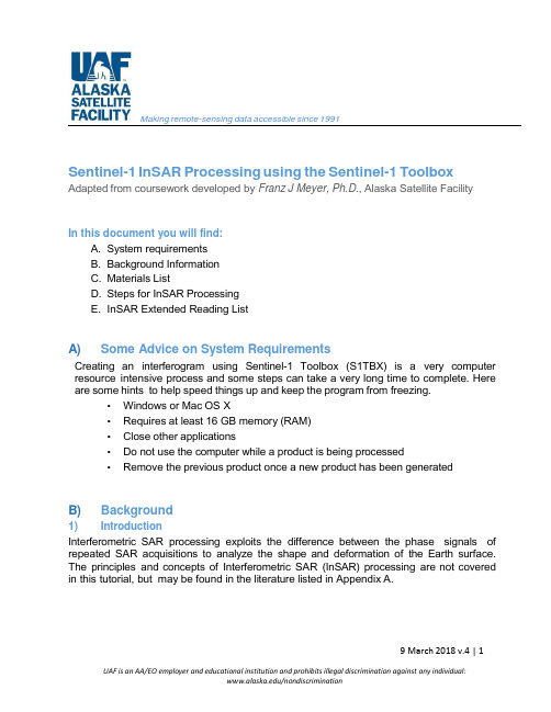
Making remote-sensing data accessible since 1991Sentinel-1 InSAR Processing using the Sentinel-1 Toolbox Adapted from coursework developed by Franz J Meyer, Ph.D., Alaska Satellite FacilityIn this document you will find:A. System requirementsB. Background InformationC. Materials ListD. Steps for InSAR ProcessingE. InSAR Extended Reading ListA) Some Advice on System RequirementsCreating an interferogram using Sentinel-1 Toolbox (S1TBX) is a very computer resource intensive process and some steps can take a very long time to complete. Here are some hints to help speed things up and keep the program from freezing.•Windows or Mac OS X•Requires at least 16 GB memory (RAM)•Close other applications•Do not use the computer while a product is being processed•Remove the previous product once a new product has been generatedB) Background1) IntroductionInterferometric SAR processing exploits the difference between the phase signals of repeated SAR acquisitions to analyze the shape and deformation of the Earth surface. The principles and concepts of Interferometric SAR (InSAR) processing are not covered in this tutorial, but may be found in the literature listed in Appendix A.The European Space Agency’s Sentinel-1A and Sentinel-1B C-band SAR sensors are delivering repeated SAR acquisitions with a predictable observation rate, providing an excellent basis for environmental analyses using InSAR techniques.In this data recipe, for demonstration purposes, we will analyze a pair of Sentinel-1 images that bracket the devastating 2016 Kumamoto earthquake, whose 6.5 magnitude foreshock and 7.0 main shock devastated large areas around Kumamoto, Japan in April 2016. Figure 1 shows the USGS ShakeMap associated with the 7.0 magnitude main shock, showing both the violence of the event and the location of the largest devastation.Figure 1: 2016 Kumamoto Earthquake, JP2) A Word on Sentinel-1 Interferometric Wide Swath (IW) DataThe Interferometric Wide (IW) swath mode is the main acquisition mode over land for Sentinel- 1. It acquires data with a 250km swath at 5m x 20m spatial resolution (single look). IW mode captures three sub-swaths using the Terrain Observation with Progressive Scans SAR (TOPSAR) acquisition principle.With the TOPSAR technique, in addition to steering the beam in range as in ScanSAR, the beam is also electronically steered from backward to forward in the azimuth direction for each burst, avoiding scalloping and resulting in homogeneous image quality throughout the swath. A schematic of the TOPSAR acquisition principle is shown below in Figure 2.The TOPSAR mode replaces the conventional ScanSAR mode, achieving the same coverage and resolution as ScanSAR, but with nearly uniform image quality (in terms of Signal-to- Noise Ratio and Distributed Target Ambiguity Ratio).IW Single Look Complex (SLC) products contain one image per sub-swath and one per polarization channel, for a total of three (single polarization) or six (dual polarization) images in an IW product.Figure 2: TOPSAR acquisition principleEach sub-swath image consists of a series of bursts, where each burst has been processed as a separate SLC image. The individually focused complex burst images are included, in azimuth-time order, into a single sub-swath image with black-fill demarcation in between, similar to ENVISAT ASAR Wide ScanSAR SLC products (see also Figure 5).3) Sentinel-1 and the Kumamoto EarthquakeThe sample images for this data recipe were acquired on April 8 and April 20, 2016, bracketing the fore and main shock of the Kumamoto earthquake event. Hence, the phase difference between these image acquisitions capture the cumulative co-seismic deformation caused by both of these seismic events. The footprint of the Sentinel-1 images (Figure 3) shows good correspondence with the areas affected by the earthquake (Figure 1).Figure 3: Footprint of the Sentinel-1A SAR data used in this data recipeC) Materials List1. Sentinel-1 Toolbox(S1TBX) Download2. Data (sample images provided)Pre event image sample:S1A_IW_SLC 1SSV_20160408T091355_20160408T091430_010728_01001F_83EB DownloadPost-event image sample:S1A_IW_SLC 1SSV_20160420T091355_20160420T091423_010903_010569_F9CE DownloadImportant: Do not unzip the downloaded files. If you are using Safari, in the top menunavigate to Safari > Preferences > General tab. Uncheck the box next to “Open safefiles after downloading” to prevent the files from automatically unzipping.Note: You will be prompted for your Earthdata Login username and password, ormust already be logged in to Earthdata before the download will begin.D) Steps for InSAR Processing∙Download software and data, and open data∙Open data in S1TBX∙Co-register the data∙Interferogram formation and coherenceo Form the interferogramo TOPS Debursto Topographic Phase Removalo Multi-looking & Phase Filteringo Geocoding & Export in a User-Defined Formato Combine subswaths – optionalDownload Software & Data, and Open Data1) Download materialsa. Download and install the S1TBX application (Select the correct version foryour operating system)b. Create a working folder for the Sentinel-1 sample images andintermediary products created during processingc. Download the sample images in Section C to the new working folder usingASF Vertex, or use the download links providedOpening Data in Sentinel-1 ToolboxStart the S1TBX application.Figure 4: Open Product dialog in Sentinel-1 Toolbox (S1TBX)In order to perform interferometric processing, the input products should be two or more SLC products over the same area acquired at different times, such as the sample images provided in this tutorial.1) Open the products –Step 1Use the Open Product button in the top toolbar and browse for the location of the Sentinel-1 Interferometric Wide (IW) SLC products (Figure 4).Important: Do not unzip the downloaded filesPress and hold the <Ctrl> button and select the files. Click <Open> to load the files into S1TBX.2) View the products –Step 2In the Product Explorer window (Figure 5) you will see the products.Double-click on each product to expand the view.Double-click Bands to expand the folder.In the Bands folder, you will find bands containing the real (i) and imaginary (q) parts of the complex data. The i and q bands are the bands that are actually in the product.The V(irtual) Intensity band is there to assist you in working with and visualizing the complex data.Figure 5: Product Explorer tab within the S1TBX user interfaceNote that in Sentinel-1 IW SLC products, you will find three subswaths labeled IW1, IW2, and IW3. Each subswath is for an adjacent acquisition by the TOPS mode.3) View a band –Step 3To view the data, double-click on the Intensity_IW1_VV band of one of the two images.Zoom in on the image and pan by using the tools in the Navigation window below the Product Explorer window. Within a subswath, TOPS data are acquired in bursts. Each burst is separated by a demarcation zone (Figure 6). Any ‘data’ within these demarcation zones can be considered invalid and should be zero-filled, but may also contain garbage values.Figure 6: Intensity image of IW1 swath with bursts and demarcationareas identifiedCo-register the DataFor interferometric processing, two or more images must be co-registered into a stack. One image is selected as the master and the other images are the ‘slaves’. The pixels in ‘slave’ images will be moved to align with the master image to sub-pixel accuracy. Coregistration ensures that each ground target contributes to the same (range, azimuth) pixel in both the master and the ‘slave’image. For TOPSAR InSAR, S-1 TOPS Coregistration is used.1) Co-register the images –Step 4Select S-1 TOPS Coregistration in the Radar menu.TOPS Coregistration consists of a series of steps:∙Reading the two data products∙Selecting a subswath with TOPSAR-Split∙Applying precision orbit correction with Apply-Orbit-File∙Conducting a DEM-assisted Back-Geocodingcoregistration All of these steps occur automatically onceprocessing starts.A window will open allowing you to set the parameters for the coregistration process(Figure 7).Figure 7: S1TBX co-registration interface∙In the Read tab, select the first product [1]. This will be your master image.∙In the Read(2) tab select the other product. This will be your ‘slave’image.∙In the TOPSAR-Split tabs, select the IW1 subswath for each of the products.∙In the Apply-Orbit-File tabs, select the Sentinel Precise Orbit State Vectors. Orbit auxiliary data contain information about the position of the satellite during the acquisition of SAR data. Orbit data are automatically downloaded by S1TBX and no manual search is required by the user.The Precise Orbit Determination (POD) service for Sentinel-1 provides Restituted orbit files and Precise Orbit Ephemerides (POE) orbit files. POE files cover approximately 28 hours and contain orbit state vectors at fixed time steps of 10-second intervals. Files are generated one file per day and are delivered within 20 days after data acquisition.If Precise orbits are not yet available for your product, you may select the Restituted orbits, which may not be as accurate as the Precise orbits but will be better than the predicted orbits available within the product.In the Back-Geocoding tab, select the Digital Elevation Model (DEM) to use and the interpolation methods. The default is the SRTM 3Sec DEM and this can be used for this tutorial. Areas that are not covered by the DEM or are located in the ocean may optionally be masked out. Select to output the Deramp and Demod phase if you require Enhanced Spectral Diversity to improve the coregistration.In the Write tab, set the Directory path to your working directory.Click <Run> to begin co-registering the data. The resulting coregistered stack product will appear in the Product Explorer window with the suffix Orb_Stack.Interferogram F ormation &C oherence E stimationThe interferogram is formed by cross-multiplying the master image with the complex conjugate of the ‘ slave’. The amplitude of both images is multiplied while their respective phases are differenced to form the interferogram.The phase difference map, i.e., interferometric phase at each SAR image pixel depends only on the difference in the travel paths from each of the two SARs to the considered resolution cell.1) Form the Interferogram –Step 5Select stack [3] in Product Explorer and selectInterferogram Formation from the Radar > Interferometric > Products menu.Through the interferometric processing flow we will try to eliminate other sourcesof error and be left with only the contributor of interest, which is typically thesurface deformation related to an event.The flat-earth phase removal is done automatically during the InterferogramFormation step (Figure 8). The flat-earth phase is the phase present in theinterferometric signal due to the curvature of the reference surface. The flat-earthphase is estimated using the orbital and metadata information and subtractedfrom the complex interferogram.Keep the default values for Interferogram Formation. Click <Run>.Visualize Interferometric PhaseOnce the interferogram product is created (product [4] in Product Explorer(appended with Orb_Stack_ifg), visualize the interferometric phase. You will stillsee the demarcation zones between bursts in this initial interferogram. This willbe removed once TOPS Deburst is applied.Figure 8: S1TBX Interferogram Formation InterfaceWhat it MeansInterferometric fringes represent a full 2π cycle of phase change. Fringes appear on an interferogram as cycles of colors, with each cycle representing relative range difference of half a sensor’s wavelength. Relative ground movement between two points can be calculated by counting the fringes and multiplying by half of the wavelength. The closer the fringes are together, the greater the strain on the ground.Flat terrain should produce a constant or only slowly varying fringes. Any deviation froma parallel fringe pattern can be interpreted as topographic variation.2) TOPS Deburst –Step 6To seamlessly join all bursts in a swath into a single image, we apply the TOPS Deburst operator from the Sentinel-1 TOPS menu.∙Navigate to the Radar > Sentinel-1 TOPS menu∙Select the S-1 TOPS Deburst step∙Keep the default values∙Click <Run>The resulting product will be appended with Orb_Stack_ifg_deb.3) Topographic Phase Removal –Step 7To emphasize phase signatures related to deformation, topographic phasecontributions are typically removed using a known DEM. In S1TBX, the Topographic Phase Removal operator will simulate an interferogram based on a reference DEM and subtract it from the processed interferogram.∙Navigate to the Radar > Interferometric > Products menu∙Select the Topographic Phase Removal stepS1TBX will automatically find and download the DEM segment required for correcting your interferogram of interest. Keep the default values and click <Run>. After topographic phase removal, the resulting product (appended with Orb_Stack_ifg_deb_dinsar) will appear largely devoid of topographic influence. Multi-looking & Phase FilteringYou will see that up to this stage, your interferogram looks very noisy and fringe patterns are difficult to discern. Hence, we will apply two subsequent processing steps to reduce noise and enhance the appearance of the deformation fringes.Interferometric phase can be corrupted by noise from:∙Temporal decorrelation∙Geometric decorrelation∙Volume scattering∙Processing errorTo be able to properly analyze the phase signatures in the interferogram, the signal-to-noise ratio will be increased by applying multi-looking and phase filtering techniques:4) Multi-looking –Step 8The first step to improve phase fidelity is called multi-looking. Navigate to the Radardropdown menu∙Select the Multilooking option (bottom of the menu). A new window opens.∙Click on the Processing Parameters tab∙Pick the i and q bands as the Source Bands to be multi-looked∙In the Number of Range Looks field, enter 6, which will result in a pixel size of about 25m (Figure 9)In essence, multi-looking performs a spatial average of a number of neighboringpixels (in our case 6x2 pixels) to suppress noise. This process comes at theexpense of spatial resolution.∙Click <Run>. The resulting product name is appended withOrb_Stack_ifg_deb_dinsar_ML.Figure 9: S1TBX Multilooking interface5) Phase Filtering - Step 9In addition to multi-looking, we perform a phase filtering step using a state-of-the art filtering approach.∙Navigate to Radar > Interferometric > Filtering∙Select Goldstein Phase Filtering∙Keep the default values and click <Run>The resulting product name is appended with Orb_Stack_ifg_deb_dinsar_ML_flt.After phase filtering, the interferometric phase is significantly improved, and the dense earthquake deformation-related fringe pattern is now clearly visible (Figure 10).Figure 10: Deformation fringes related to the 2016 Kumamoto Earthquake show clearlyafter multi-looking and phase filtering were applied. Contains modified CopernicusSentinel data (2016) processed by ESAGeocoding & Export in a User-defined FormatTo make the data useful to geoscientists, the interferometric phase image needs to be projected into a geographic coordinate system using a DEM-assisted geocoding step.6) Geocoding - Step 10To geocode the interferometric data∙Navigate to Radar > Geometric > Terrain Correction∙Select Range-Doppler Terrain CorrectionIn the Range-Dopper Terrain Correction window (Figure 11), select product [8](or the product generated in the previous step) as Source ProductFigure 11: S1TBX Range-Doppler Terrain Correction interfaceIn Processing Parameters∙Select the Intensity and Phase images as Source Bands to be geocoded∙Adjust the pixel spacing if you want (e.g., 30m)∙Click <Run>The resulting product name is appended with Orb_Stack_ifg_deb_dinsar_ML_flt_TC.See Figure 12 for the resulting geocoded interferogram of sub-swath IW1.Figure 12: Geocoded IW1 interferogram. Contains modified CopernicusSentinel data (2016) processed by ESA7) Export Data - Step 11The final geocoded data can be exported from S1TBX in a variety of formats. To find the export options navigate to File/ExportIn addition to GeoTIFF and HDF5 formats, KMZ and various specialty formats are supported. Figure 13 shows a KMZ-formatted interferogram overlaid on Google Earth.Figure 13: Geocoded Kumamoto interferogram projected onto Google Earth. Contains modifiedCopernicus Sentinel data (2016) processed by ESACombining Subswaths –OptionalCreate a Geocoded Differential Interferogram of the Kumamoto Earthquake by Merging Subswaths IW1 and IW2To create the merged product, run the steps below, noting the new step.∙Run Step 4 - Coregistration This time select IW2 in the TOPS Split operator tab t o coregister an InSAR pair for subswath IW2 [Note: make sure to create a new filename under the “Write” tab to avoid overwriting the IW1 stack result] ∙Run S t e p 5 - Interferogram Formation Using the new coregistered IW2 stack as input, create an IW2 subswath interferogram∙Run Step 6 - Debursting Deburst the IW2 interferogram∙NEW STEP: Run Burst Merge This step combines the previously generated debursted IW1 interferogram with the newly generated debursted IW2 interferogram. To run burst merge, go to the Radar > Sentinel-1 TOPS menu and select the S-1 TOPS Merge step. Select the debursted IW1 (Orb_Stack_ifg_deb) and debursted IW2 interferograms as inputs.∙Run Steps 7-11 to create the merged productInterferogram InterpretationThe interferometric phase carries a wealth of information about surface deformation (strength and direction of motion) and the location of the surface rupture. The phase map is also a proxy for other earthquake-related parameters such as the energy released during an event and the amount of shaking experienced across the affected area.E) InSAR Extended Reading ListSummary Articles about SAR:▪Moreira, A., Prats-Iraola, P., Younis, M., Krieger, G., Hajnsek, I., & Papathanassiou, K.P. (2013). A tutorial on synthetic aperture radar. IEEE Geoscience andRemote Sensing Magazine, 1(1), 6-43.▪Rosen, P. A., Hensley, S., Joughin, I. R., Li, F. K., Madsen, S. N., Rodriguez, E., & Goldstein, R. M. (2000). Synthetic aperture radar interferometry. Proceedingsof the IEEE, 88(3), 333-382.▪Bamler, R., & Hartl, P. (1998). Synthetic aperture radar interferometry.Inverse problems, 14(4), R1.▪Bürgmann, R., Rosen, P. A., & Fielding, E. J. (2000). Synthetic aperture radar interferometry to measure Earth’s su r face topography and its deformation. Annual review of earth and planetary sciences, 28(1), 169-209.▪Simons, M., and P. A. Rosen (2007), Interferometric synthetic aperture radar geodesy, in Geodesy, Treatise on Geophysics, vol. 3, edited by T. Herring, pp.391–446, Elsevier.Interesting Articles by Topic:InSAR Processing▪Rosen, P. A., Hensley, S., Joughin, I. R., Li, F. K., Madsen, S. N., Rodriguez,E.,& Goldstein, R. M. (2000). Synthetic aperture radar interferometry.Proceedings of the IEEE, 88(3), 333-382.▪Bamler, R., & Hartl, P. (1998). Synthetic aperture radar interferometry.Inverse problems, 14(4), R1.▪Bürgmann, R., Rosen, P. A., & Fielding, E. J. (2000). Synthetic aperture radar interferometry to measure Earth’s surface topography and its deformation.Annual review of earth and planetary sciences, 28(1), 169-209.Volcanic Source Modeling Using InSAR▪Mogi, K. (1958), Relations between the eruptions of various volcanoes and the deformations of the ground surfaces around them, Bull. EarthquakeResearch Inst., 36, 99–134.▪Lohman, R. B., & Simons, M. (2005). Some thoughts on the use of InSAR data to constrain models of surface deformation: Noise structure and datadownsampling. Geochemistry, Geophysics, Geosystems, 6(1).▪Lu, Z. (2007). InSAR imaging of volcanic deformation over cloud-prone areas–Aleutian Islands. Photogrammetric Engineering & Remote Sensing,73(3), 245- 257.▪Lu, Z., & Dzurisin, D. (2010). Ground surface deformation patterns, magma supply, and magma storage at Okmok volcano, Alaska, from InSAR analysis: 2.Coeruptive deflation, July–August 2008. Journal of Geophysical Research: SolidEarth, 115(B5).▪Lu, Z., Masterlark, T., & Dzurisin, D. (2005). Interferometric synthetic aperture radar study of Okmok volcano, Alaska, 1992–2003: Magma supply dynamicsand postemplacement lava flow deformation. Journal of Geophysical Research:Solid Earth, 110(B2).▪Baker, S., & Amelung, F. (2012). Top‐down inflation and deflation at the summit of Kīlau ea Volcano, Hawai ‘i observed with InSAR. Journal of GeophysicalResearch: Solid Earth, 117(B12).▪Wright, T. J., Lu, Z., & Wicks, C. (2003). Source model for the Mw 6.7, 23 October 2002, Nenana Mountain Earthquake (Alaska) from InSAR. GeophysicalResearch Letters, 30(18). [Supplements]InSAR Time Series Analysis▪Ferretti, A., Prati, C., & Rocca, F. (2001). Permanent scatterers in SAR interferometry. IEEE Transactions on geoscience and remote sensing, 39(1), 8-20.▪Berardino, P., Fornaro, G., Lanari, R., & Sansosti, E. (2002). A new algorithm for surface deformation monitoring based on small baseline differential SARinterferograms. IEEE Transactions on Geoscience and Remote Sensing, 40(11),2375-2383.▪Lanari, R., Mora, O., Manunta, M., Mallorquí, J. J., Berardino, P., & Sansosti, E.(2004). A small-baseline approach for investigating deformations on full-resolution differential SAR interferograms. IEEE Transactions on Geoscienceand Remote Sensing, 42(7), 1377-1386.▪Hooper, A., Segall, P., & Zebker, H. (2007). Persistent scatterer interferometric synthetic aperture radar for crustal deformation analysis, with application toVolcán Alcedo, Galápagos. Journal of Geophysical Research: Solid Earth,112(B7).▪Ferretti, A., Fumagalli, A., Novali, F., Prati, C., Rocca, F., & Rucci, A. (2011). A new algorithm for processing interferometric data-stacks: SqueeSAR. IEEETransactions on Geoscience and Remote Sensing, 49(9), 3460-3470.。
航测数据后处理软件及方法推荐
航测数据后处理软件及方法推荐航测数据的后处理在测绘领域中扮演着至关重要的角色。
通过对航测数据的处理和分析,可以得到精确、高质量的地理信息数据,为地理信息系统、土地规划、资源管理等领域提供可靠的数据支持。
本文将推荐几款常用的航测数据后处理软件和方法,并探讨其适用场景和优劣势。
一、航测数据后处理软件1. ENVIENVI是一款功能强大的遥感图像分析软件,具有图像处理、分类、变化检测、目标识别等多种功能。
在航测数据的后处理中,ENVI可以用于影像配准、地物分类和高程模型生成。
它提供了丰富的算法和工具,能够处理不同分辨率的航测数据。
2. Pix4DmapperPix4Dmapper是一款专业的无人机航测数据处理软件,主要用于无人机航测数据的处理和三维建模。
它可以将无人机采集到的航测图像进行自动配准和拼接,生成高精度的地形模型和三维模型。
Pix4Dmapper还提供了丰富的分析工具,可以进行体积计算、变形分析等操作。
3. Erdas ImagineErdas Imagine是一款功能全面的遥感图像处理软件,主要用于航测数据的处理、分析和制图。
它支持多种数据格式,包括数字摄影测量系统(DGPS)、激光雷达、航空摄影等。
Erdas Imagine具有强大的图像处理和分析功能,可以进行几何校正、影像融合、地物提取等操作。
二、航测数据后处理方法1. 影像配准航测数据中的图像可能存在位置偏差和旋转,需要进行影像配准以消除这些误差。
影像配准可以采用基于特征匹配的方法,如SIFT、SURF等,也可以使用控制点进行配准。
其中,SIFT是一种基于局部特征的图像配准算法,可以自动提取图像中的稳定特征点,并通过匹配这些特征点来实现图像配准。
2. 高程模型生成航测数据中的高程信息对于地理信息系统和土地规划非常重要。
高程模型可以通过航测数据中的点云数据或影像进行生成。
常用的高程模型生成方法包括插值法和立体视差法。
插值法可以通过对离散的高程数据进行插值,得到连续的地形表面。
干涉SAR加权定标方法
3. WEIGHTED CALIBRATE METHOD
Interferometric phase noise, which can be computed from correlation coefficients, varies from point to point, so the sensitivity equations of each control point have different errors. Therefore, it is reasonable to introduce different weightings to these sensitivity equations. With the weightings, solving (2) is equal to make F 'X - 'H ȁ minimum, and it is expressed by (7).
where 'X
> 'B 'D 'I 'r 'H @
T
, F is the sensitivity
matrix, 'H is the elevation differences between the control point and the corresponding pixel in a SAR DEM. F and 'H can be expressed as wh wh wh wh º ª wh 1 1 1 1 1 wD wI wr wH » ª F1 º « wB « » « » F « » « » (3) « » « wh wh wh wh » ¬ FN » ¼ « wh N N N N N « wD wI wr wH » ¬ wB ¼
TerraSAR-X高分辨率雷达卫星数据介绍
hsatellite
带宽Bandwidth 数据收集范围Data collection range 全效率范围Full performance range
高分辨率SpotLight模式
High Resolution SpotLight Mode
10 km x 10 km 1-4 m 取决于入射角和多极化方式 单极化 (VV or HH) 双极化 (HH/VV) 150 and 300 MHz 15° to 60° 20° to 55° 5 x 10 km
StripMap 模式StripMap mode
30km幅宽30 km swath 3m分辨率3 m resolution
高分辨率&SpotLight模式
High Resolution & SpotLightmode
5/10 km x 10 km 1m分辨率1 m resolution
双重天线接收模式Dual receive antenna mode
卫星轨道
Satellite orbit
hsatellite
空间分辨率Spatial resolution 极化方式Polarization
星下轨迹
Nadir track
Θ1=2
0o
数据收集范围Data collection range 全效率区域Full performance range
30 km (单极化) 15 km (双极化) 50 km 4,200 km technical, 1.650 km acc. to product spec. 3 m (单极化), 6 m(双极化) Single (VV or HH) Dual (HH/VV, HH/HV, VV/VH) Quad (HH/VV/HV/VH) 15° to 60° 20° to 45°
GAMMA-ISP
1引言GAMMA雷达干涉测量处理程序包含一套完整的算法,这些算法对于生成干涉图、高程图、相干图和差分干涉产品是必须的。
程序步骤包括由轨道数据估计基线,干涉影像对的精密配准,干涉图的生成(包括公共带滤波),干涉相干性估计,平地效应的去除,干涉图的自适应滤波,相位解缠,由地面控制点精确估计干涉基线,高程图的生成,影像纠正和干涉高程图的插值。
此外,ISP还提供了用于SLC辐射定标以及斜距和地距之间转换的程序。
另外ISP还支持PRI/MLI数据的处理,这些数据代表SAR图像的强度信息。
其中,PRI代表精确图像,它是在频率域通过多视次波段的原始数据获得的,PRI 图像是地距结构的。
MLI代表多视强度图像,它是在空间域通过无条理地平均SLC 和PRI数据距离向和方位向的领域像元值获得的,依据是否平均SLC和PRI图像,相应的MLI图像要么是斜距结构,要么是地距结构。
MLI图像是由浮点型数据组成,图像的宽和高由距离向和方位向选择的视数确定。
SLC/PRI/MLI数据要么是采用GAMMA软件的MSP模块处理原始数据得到的,要么是从数据处理商那里购买的。
ISP软件包的处理程序都支持这两种格式的数据。
干涉测量处理将产生一批图像产品:干涉图(复数数据),解缠图像,相干图像和强度图像(都是实数数据)。
首先准备的数据必须能够满足GAMMA软件支持的格式。
为了克服这个困难,对大多数SAR数据产品都采用CEOS格式,ISP软件包(包括其它的GAMMA软件包)采用一个简单的数据结构,元数据在头文件里面,还有一个图像数据。
处理相关参数和SAR数据特点储存在一个text文件里面。
文件用和系统参数有关的简单的关键字命名的。
文件的结构能够采用ISP程序初始化和改正。
输出的文件称作ISP SLC参数文件。
预处理步骤外的其他操作包括轨道状态向量的处理和定标。
如果分析的是PRI/MLI数据,那么定标这一步尤其重要。
ISP还包含了从SLC数据生成MLI数据,SLC、PRI和MLI数据的辐射定标,SLC重采样和斜距到地距之间相互转换的程序。
- 1、下载文档前请自行甄别文档内容的完整性,平台不提供额外的编辑、内容补充、找答案等附加服务。
- 2、"仅部分预览"的文档,不可在线预览部分如存在完整性等问题,可反馈申请退款(可完整预览的文档不适用该条件!)。
- 3、如文档侵犯您的权益,请联系客服反馈,我们会尽快为您处理(人工客服工作时间:9:00-18:30)。
GAMMA SAR AND INTERFEROMETRIC PROCESSING SOFTWARECharles Werner, Urs Wegmüller, Tazio Strozzi and Andreas WiesmannGamma Remote Sensing, Thunstrasse 130, CH-3074 Muri b. Bern, Switzerland Tel: +41 31 951 70 05, Fax: +41 31 951 70 08, Email: cw@gamma-rs.ch, http://www.gamma-rs.chABSTRACTThe GAMMA Modular SAR Processor (MSP), Interferometric SAR Processor (ISP), Differential Interferometry and Geocoding Software (DIFF&GEO), and Land Application Tools (LAT) are modular software packages useful to process synthetic aperture radar (SAR) images. Data of both spaceborne and airborne sensors including ERS-1/2, JERS-1, SIR-C, SEASAT, RADARSAT StripMap mode, and the single-pass Dornier DOSAR interferometer have been successfully processed interferometrically. State of the art algorithms have been implemented to achieve accurate processing of the data while permitting timely processing of large data sets. Recent projects completed with the software include generation of a continental scale mosaic of Siberia consisting of more 700 JERS scenes in the frame of the SIBERIA project and the generation of subsidence maps for Bologna, Abano, and Mexico City. User-friendly display tools and full documentation in HTML language complements the software. Both binary and source code licenses are available. Recent developments included the adaptation of the software to the PC operating systems LINUX and NT and the improvement of the functionality for differential SAR interferometry. Furthermore, as part of our ERS AO3 project (ERS AO3-175), software demonstration, training, and testing examples have been developed for distribution to users. Development in the near future will include the adaptation of the software to the processing of ENVISAT ASAR (with data provided through ENV AO-210) and ALOS PALSAR (ALOS AO proposal accepted) data.Keywords: SAR processing, SAR interferometry, GAMMA Software, ERS, ENVISAT, ALOSINTRODUCTIONGAMMA Remote Sensing Research and Consulting AG (GAMMA) is a Swiss corporation (Aktiengesellschaft - AG) founded in January 1995 and located near Bern, Switzerland. Research and development, processing and adding value to remote sensing data, license sales for its commercial processing software, and EO-data distribution are GAMMA's primary business elements. GAMMA's declared goal is to maintain a high level of technical and scientific expertise. This is an essential prerequisite for development of new applications, consulting activities, and improving and maintaining the commercial software. To achieve this ambitious goal GAMMA is involved in research projects (ESA, EC, National Projects, etc.) and cooperates with competent partners at universities, public institutes and private companies.Research and development on new processing techniques is essential to maintaining the advanced level of GAMMA's processing software. GAMMA's competence encompasses technical aspects such as SAR processing, interferometry, differential interferometry, geocoding, and mosaicing as well as fully integrated product generation from EO-data. Typical products are digital elevation models, geophysical displacement maps and landuse products (forest maps, hazard maps, etc.). Pull factors driving GAMMA's R&D on processing techniques originate from demands of existing and new applications, the optimization of the techniques for new sensors, operational requirements, and quality control. New developments presented at conferences and in the literature and new hardware and software are relevant push factors to advance GAMMA's in-house technology. Recent examples include development of new methods for SAR geocoding, glacier velocity mapping, interferogram stacking, and phase unwrapping.SYSTEM OVERVIEWGAMMA provides licenses for its user-friendly and high quality software to support the entire processing from SAR raw data to high level products such as digital elevation models, deformation, and landuse maps. The software is grouped into four packages:• Modular SAR Processor (MSP) – processing of raw SAR data to calibrated SLC and backscatter products• Interferometric SAR Processor (ISP) – generation of interferometric products such as correlation maps, interferograms, unwrapped phase, and height maps.• Differential Interferometry and Geocoding (DIFF&GEO) – generation of geocoded and differential interferometric products• Land Application Tools (LAT) – classification and image analysis toolsThe software is written in ANSI-C and has been installed on different UNIX workstations and on PC platforms with LINUX or NT operation systems. Documentation is provided in HTML language. Both binary and source code licenses are available. Attractive discounts are offered for University / Education users.Each of the packages is very modular. The offered alternatives and parameters read from the command line allow optimization of the processing for specific cases. Shell scripts (e.g. csh, Perl) permit running and documentation of processing sequences in an operational and efficient way. Full frame SAR processing times for ERS and JERS on today's workstations and PCs are well below one hour. The software processes data of spaceborne and airborne SAR, including ERS-1/2, JERS, RADARSAT, and SIR-C. It fully supports the data formats provided by the different space agencies. Parameter estimation and quality control programs complement the main processing sequences. For example a point target analysis is included in the SAR processing suite for verification of processing performance. A complete suite of display programs and utilities based on open source technology are added for convenient access to the input data, intermediate products, and final results.MODULAR SAR PROCESSOR (MSP)The GAMMA Modular SAR Processor (MSP) is a flexible, accurate range-Doppler SAR processor [1]. It allows the generation of complex and real-valued SAR images from raw data of the current generation of spaceborne and airborne sensors. The processing includes radiometric calibration and is phase preserving for interferometric processing. Parameters relating to processing and data characteristics are saved as text files with system parameters referenced using simple keywords. The main modules of the MSP are pre-processing and data conditioning, range compression with optional azimuth prefiltering, autofocus, azimuth compression, and multi-look post processing (flow chart see Figure 4). The processed images are radiometrically normalized for the antenna pattern, along-track receiver gain variations, length of the azimuth and range reference functions, and slant range. Multilook images are produced by time-domain averaging of the single look complex image samples. Special features to optimize the processing of data of the current spaceborne sensors are autofocus (all SAR sensors), radio interference filtering (JERS), Doppler ambiguity estimation (JERS, RADARSAT), missing line detection (ERS-1/2, Figure 1), and secondary range migration (JERS, RADARSAT, Figures2,3). An advanced motion compensation module is also available for processing of airborne SAR data.Figure 1. ERS-1 Death Valley: The GAMMA Modular SAR Processor (MSP) rapidly processes full frames to full resolution and includes programs for the assessment of data quality and processing parameters.Raw data courtesy of ESA. Processing by GAMMA.Figure 2. RADARSAT ("fine beammode"), Bar Harbor, Maine. GAMMAMSP supports processing of allRADARSAT strip map modes.Raw data courtesy of RSI, Canada.Processing by GAMMA.Figure 3. JERS-1, Mount Fuji (Japan):Multi-look intensity image. JERSProcessing includes Doppler ambiguityestimation and RFI filtering.Raw data courtesy of NASDA, Canada.Processing by GAMMA.Figure 4. GAMMA Modular SAR Processor (MSP): Flow ChartINTERFEROMETRIC SAR PROCESSOR (ISP)The interferometric processor gives end to end support in the generation of interferometric products starting with complex SAR data as the SLC products provided by the Processing and Archiving Facilities (PAFs) or as processed by the GAMMA MSP [1]. The different modules include:• baseline estimation from orbit data• precision registration of interferometric image pairs• interferogram generation (including common spectral band filtering)• coherence estimation of the interferogram• removal of curved Earth phase trend (interferogram phase flattening)• adaptive filtering of interferograms• phase unwrapping using a branch cut algorithm• precision estimation of interferometric baselines from ground control points• derivation of topographic height• image rectification and interpolation of interferometric height and slope mapsA flow chart for typical interferometric processing is shown in Figure 5. The display of the final and intermediate products is supported with screen display programs and programs to generate easily portable images in SUN rasterfile and BMP format. Processing related parameters and data characteristics are saved as text files that can be displayed using commercial plotting packages. The main processing sequence is complemented by quality control and display programs.Examples for interferometric height maps (Figures 6,7) and coherence-backscatter-change composites (Figure 8,9) areFigure 5. GAMMA Interferometric SAR Processor (ISP): Flow ChartFigure 6. DOSAR, near Solothurn (Switzerland): interferometric height map over agriculture/forest site. SAR processing, motion compensation, and interferometric processing with GAMMA MSP and ISP. DOSAR data courtesy of Dornier GmbH and RSL Univ. Zürich.Figure 7. SIR-C, Amazon (Columbia): Interferometric height map generated from SIR-C (L-Band, vv polarization) data for a tropical forest test-site. Interferometric processing with GAMMA ISP.SIR-C SLC data courtesy of JPL/NASA.Figure 8. JERS mosaic SIBERIA: A 40 x 34 km2 sectionof a large JERS mosaic over Siberia, includinginterferometric coverage as shown above.Raw data courtesy of DLR and NASDA, Processing byGAMMA.Figure 9. SIR-C, Yverdon (Switzerland): SAR interferometric landuse characterization generated from SIR-C (C-Band, vv polarization) data. Color composite of the interferometric correlation (red), backscatter intensity (green), and backscatter change (blue). Interferometricprocessing with GAMMA ISP .SIR-C SLC data courtesy of JPL/NASA. Processing byGAMMA.GAMMA DIFFERENTIAL INTERFEROMETRY AND GEOCODING SOFTWARE (DIFF&GEO )The GAMMA Differential Interferometry and Geocoding Software (DIFF&GEO ) is a suite of programs designed to support differential interferometric processing as well as conversion between range-Doppler coordinates and various map projections. The reason for inclusion of these quite different processes into one software module is that geocoding capability is required for 2-pass differential interferometry where a DEM projected into SAR range-Doppler coordinates is used to generate a synthetic interferogram.Geocoding: Geocoding is the coordinate transformation between the coordinates of an imaging system, in this case range-Doppler coordinates of the SAR, and orthonormal map coordinates. Geocoding is necessary to combine information retrieved by the imaging system (e.g. the SAR image and products derived from it) with information in map coordinates (e.g. a digital elevation model, a landuse inventory, geocoded information from optical remote sensing)[2].Figure 10 shows a flow chart characterizing different geocoding approaches supported by the software.Figure 10. GAMMA DIFF&GEO Software: Geocoding Flow ChartFigure 11. GAMMADIFF&GEO Software: Flow Chart showing Differential Interferometry ApproachesFigure 12. Subsidence map of the urban area of Bologna from ERS differential interferometry. One color cycle corresponds to a subsidence velocity of 1 cm/year starting from the stable base of the Appenini (in the south). Data processing with GAMMA MSP, ISP, and DIFF&GEO. ERS raw data courtesy of ESA.Figure 13. Mexico City: Contour lines of equal ground sinking velocity based on leveling campaigns in 1994 and 1996 (provided by Vega) superimposed on the ERS SAR interferometric subsidence map calculated for the second half of 1996. One color cycle corresponds to 5cm/year subsidence.Differential Interferometry: The interferometric phase is sensitive to both surface topography and coherent displacement in between the acquisitions of an image pair. The basic idea of differential interferometric processing is to separate the two effects, allowing, in particular, to retrieve a differential displacement map. This goal is achieved by subtracting the topography-related phase. The topography related phase could either be calculated from a conventional DEM (2-pass differential interferometry) or from an independent interferometric pair without phase component from differential displacement (3- and 4-pass differential interferometry). Various approaches are supported by the DIFF&GEO leading to high flexibility with respect to the availability of data (DEM, SAR) and the feasibility of phase unwrapping [3] (Figure 11). Figures 12 and 13 show recent results of mapping subsidence over Bologna and Mexico City using ERS data [4], [5].GAMMA LAND APPLICATION TOOLS (LAT)The GAMMA Land Application Tools (LAT) are a collection of programs designed to support data processing in the context of using SAR and SAR interferometry for land applications. The LAT includes special programs for filtering, parameter estimation, and data visualization. There are programs to select test areas, and to extract the corresponding signatures. In addition, the LAT supports simple classification schemes and image mosaicking. Examples for results areshown in Figures 14 and 15.Figure 14. ERS-1, Flevoland (The Netherlands): RGB composite figure of the interferometric correlation of the September 19 / October 4 (red), October 4 / October 19 (green), and October 19 / November 9 (blue) 1991 pairs. ERS data courtesy of ESA, Processing by GAMMA.Figure 15. Landuse map for a part of Switzerland derived with ERS SAR interferometry. Data processing with GAMMA MSP, ISP, DIFF&GEO, and LAT. ERS raw data courtesy of ESA. Processing by GAMMA.DISPLAY TOOLS (DISP)Essential for making full use of the Gamma software is a set of tools that can display results on the screen and produce raster image products for documentation and archive purposes. The programs within the DISP package are organized by the data type and display functionality. Supported input data include:• raw SAR data and byte images• single look complex (SLC) and detected multi-look intensity SAR images• interferograms, unwrapped phase, and interferometric correlation• DEMs and interferometric height maps showing both geographic and map-projection coordinates.• Differential interferometric products such as subsidence maps• Display and editing of phase unwrapping flag files• 8 and 24 bit SUN and BMP raster image format filesWithin the DISP package are also programs for display of multiple data sets, either by merging the data, such as combining intensity and interferometric phase, or rapidly flickering between images of the same type. Each screen display program can access the original data files to extract the data values at the cursor position (Figure 16). The cursorcoordinates are calculated in map projection coordinates when DEM or raster data are in a map projection format such as UTM (Figure 17). Graphical editing of the files used to support phase unwrapping is also supported.The screen display programs were developed using the open source GTK+ toolkit () that can be compiled to run both under the X or Win32 98/NT/2000 graphic environment. Therefore the user has the same display functionality if running either a Linux or Win32 operating system on an X86 compatible platform.The screen display and raster image generation programs are parallel in terms of functionality. For example, the program for screen display of detected intensity images is called dispwr, while the program for generation of a raster image of the same data set is called raspwr. Most of the raster image programs support multi-looking in both range and azimuth. The images produced can be displayed using either the DISP program disras or other raster image file viewer such as xv or Photoshop.Figure 16. Display of DEM using shaded relief scaling. Latitude and longitude together with the UTM coordinates are displayed for the point in the zoom window Figure 17. Display of complex interferogram and intensity images showing main image window, zoom window, data values, and color table selection menu.SUPPORT AND MAINTENANCEFor the purposes of testing, training and demonstration the GAMMA software, processing examples consisting of the required input data, shell scripts to run the processing sequences, and copies of the expected results for validation of the successful processing, have been generated. These examples cover typical processing sequences as often used for SAR processing, interferogram generation, coherence estimation, height mapping, differential interferometry and geocoding. Shell scripts provided with the test data implement entire processing sequences and demonstrate efficient application of the software to users. On the other hand each command can be executed separately which helps the users to understand the role and functionality of each processing step. The data used for these examples was kindly provided by ESA as part of our ERS-AO3 175 project. Permission to distribute these data for the above mentioned use was also given by ESA SUPPORT OF FUTURE MISSIONSThe modular construction of the software permits rapid integration of support for future SAR instruments and missions including the ENVISAT ASAR and ALOS PALSAR missions planned for launch within the next few years. These missions will be characterized by an increased number of mapping modes and polarisations. The Gamma software currently supports Radarsat-1, which is similar with regard to having a multiple mapping modes. These sensors will also have improved orbit knowledge and control that will have a significant impact on interferometry applications. Gamma has already been approved by ESA under AO project 210 and NASDA to have access to data raw data for upgrading the software and calibration purposes and it is our intention to provide upgraded software as soon as possible after launch. CONCLUSIONSWith its functionality, flexibility, robustness, efficiency, and competitive price, GAMMA software is an excellent solution for demanding processing jobs. This has been demonstrated by license sales to users at many leading institutes world-wide, since 1995. A distinct advantage of the GAMMA software is the competent user support provided directly by the developers and experienced users of the software. This software is an essential backbone of GAMMA's researchand value adding effort. New algorithms developed in-house and as reported at conferences and the open literature are evaluated for inclusion in the Gamma Software and the modular structure and availability of source code licenses allows users to easily implement and integrate their own processing modules.Recent software developments includes: full functionality on workstations (UNIX) and PCs (LINUX, NT), use of faster FFT routines to further reduce processing times, improved display tools using GTK with full portability to PCs (LINUX and Win32 98/NT/2000). The functionality, flexibility, and accuracy of the offset estimation programs was further enhanced to allow coherence and feature tracking for monitoring of fast glacier motion and large seismic displacements. Information on the software may be found at GAMMA's homepage: http://www.gamma-rs.ch and in GAMMA's Brochure GAMMA SAR AND INTERFEROMETRY SOFTWARE.ACKNOWLEDGMENTSParts of the ERS data used for this work were kindly made available by ESA in the frame of the ERS Announcement of Opportunity Projects ERS-AO3-175 and ERS-AO3-178.REFERENCES[1]Wegmüller U. and T. Strozzi, (1998), SAR interferometric and differential interferometric processing chain. Proc.IGARSS'98, Seattle, USA.[2] Wegmüller U., Automated terrain corrected SAR geocoding, Proceedings of IGARSS'99, Hamburg, 28 June - 2July 1999 (CC03_02)[3]Wegmüller U. and T. Strozzi (1998), Characterization of differential interferometry approaches, EUSAR'98, 25-27May, Friedrichshafen, Germany, VDE-Verlag, ISBN 3-8007-2359-X, pp. 237-240.[4]Strozzi T., U. Wegmüller, and G. Bitelli (2000), Differential SAR interferometry for land subsidence mapping inBologna, Proc. SISOLS'2000, Ravenna, Italy, 25-29 September.[5]Strozzi T. and U. Wegmüller (1999), Land Subsidence in Mexico City Mapped by ERS Differential SARInterferometry, Proc. IGARSS'99, Hamburg, 28 June - 2 July.。