On the measurement of the proton-air cross section using longitudinal shower profiles

合集下载

H.Jesse Smith 1999 Nature Dual modes of the carbon cycle since the Last Glacial Maximum

letters to nature8.Leznoff,C.C.&Lever,A.B.P.(eds)Phthalocyanines:Properties and Applications(VCH,New York,1989).9.Wang,L.S.,Ding,C.F.,Wang,X.B.&Barlow,S.E.Photodetachment photoelectron spectroscopy ofmultiply charged anions using electrospray ionization.Rev.Sci.Instrum.70,1957±1966(1999). 10.Berkowitz,J.Photoelectron spectroscopy of phthalocyanine vapors.J.Chem.Phys.70,2819±2828(1979).11.Brown,C.J.Crystal structure of b-copper phthalocyanine.J.Chem.Soc.A2488±2493(1968).12.Rosa,A.&Baerends,E.J.Metal-macrocycle interaction in phthalocyanines:density functionalcalculations of ground and excited states.Inorg.Chem.33,584±595(1994).13.PC Spartan Plus5.1(Wavefunction,Inc.,Von Carman Ave.,Irvine,California92612,USA).14.Stewart,J.J.Optimization of parameters for semiempirical methods II:put.Chem.10;221±264(1989);MOPAC:A semiempirical molecular orbital put.Aided Mol.Design4;1±105(1990).15.D'Haennens,I.J.in Encyclopedia of Physics(eds Lerner,R.G.&Trigg,G.L.)1251±1253(VCH,NewYork,1991).16.Hodgson,P.E.,Gadioli,E.&Erba,E.G.Introductory Nuclear Physics(Clarendon,Oxford,1997).17.Scheller,M.K.&Cederbaum,L.S.A construction principle for stable multiply charged molecularanions in the gas phase.Chem.Phys.Lett.216,141±146(1993).18.Weikert,H.-G.&Cederbaum,L.S.Free doubly negative tetrahalides.J.Chem.Phys.99,8877±8891(1993).19.Boldyrev,A.I.,Gutowski,M.&Simons,J.Small multiply charged anions as building blocks inchemistry.Acc.Chem.Res.29,497±502(1996).20.Vekey,K.Multiply charged ions.Mass Spectrom.Rev.14,195±225(1995).21.Brechignac,C.,Cahuzac,P.,Kebaili,N.&Leygnier,J.Temperature effects in the Coulombic®ssion ofstrontium clusters.Phys.Rev.Lett.81,4612±4615(1998).22.Schroder,D.,Harvey,J.N.&Schwarz,H.Long-lived,multiply charged diatomic TiF n+ions(n=1±3).J.Phys.Chem.A102,3639±3642(1998).Acknowledgements.We thank R.S.Disselkamp for discussions and K.Ferris for help in the theoretical calculations.This work was supported by the US Department of Energy,Of®ce of Basic Energy Sciences, Chemical Sciences Division and is conducted at the Paci®c Northwest National Laboratory,operated for the US Department of Energy by Battelle Memorial Institute.L.-S.W.is an Alfred P.Sloan research fellow.Correspondence and requests for materials should be addressed to L.-S.W.(e-mail:ls.wang@).Dual modes of thecarbon cycle since theLast Glacial MaximumH.Jesse Smith*,H.Fischer*²,M.Wahlen*,D.Mastroianni* &B.Deck**Scripps Institution of Oceanography,University of California San Diego,La Jolla,California92093-0220,USA ......................................................................................................................... The most conspicuous feature of the record of past climate contained in polar ice is the rapid warming which occurs after long intervals of gradual cooling.During the last four transitions from glacial to interglacial conditions,over which such abrupt warmings occur,ice records indicate that the CO2concentration of the atmosphere increased by roughly80to100parts per million by volume(refs1±4).But the causes of the atmospheric CO2 concentration increases are unclear.Here we present the stable-carbon-isotope composition(d13CO2)of CO2extracted from air trapped in ice at Taylor Dome,Antarctica,from the Last Glacial Maximum to the onset of Holocene times.The global carbon cycle is shown to have operated in two distinct primary modes on the timescale of thousands of years,one when climate was changing relatively slowly and another when warming was rapid,each with a characteristic average stable-carbon-isotope composition of the net CO2exchanged by the atmosphere with the land and oceans. d13CO2increased between16.5and9thousand years ago by slightly more than would be estimated to be caused by the physical effects of a58C rise in global average sea surface temperature driving a CO2ef¯ux from the ocean,but our data do not allow speci®c causes to be constrained.Carbon dioxide in the atmosphere causes a radiative forcing second only to water vapour,and so may be a central agent in climate change.Polar ice cores contain a detailed record of climate-²Present address:Alfred-Wegener-Institute for Polar and Marine Research,Columbusstrasss,D-27515 Bremerhaven,Germany.related variables which extends more than400,000years into the past4,and are especially valuable for studying variations of atmos-pheric CO2as they contain an effectively direct record,unlike atmospheric proxies such as marine carbonates or preserved organic material5which may also re¯ect biological effects.Ice cores from Antarctica,such as those of Taylor Dome and Vostok, are the best sources for palaeoatmospheric CO2measurements because they contain only small amounts of the kinds of chemical impurities,such as carbonate dust or organic acids,that may lead to contamination by in situ CO2production2,6±8.Taylor Dome ice has the additional advantage that the entire554-m-long core is from above the depth at which air trapped in bubbles in the ice forms gas±ice clathrates.This feature is important because,as we have found,the accuracy of d13CO2measurements performed on bubble-free ice may be affected by the presence of clathrates.(d13C is de®ned in Methods.)We have measured the CO2concentration and d13CO2 of air trapped in ice from Taylor Dome,Antarctica,across the last glacial termination in order to develop a time series for the carbon-isotope composition of atmospheric CO2and to constrain the mechanisms of carbon cycling between the main sources and sinks of atmospheric CO2.The atmospheric CO2concentration data3,9(Fig.1)form a record comparable to that from Byrd and Vostok1,2.The salient features include a low but variable concentration of atmospheric CO2 between27.1and18.0kyr BP(thousand years before present, where``present''is de®ned as AD1950),when it varied between 186and201parts per million by volume(p.p.m.v.);a rise,at a fairly constant rate,from190p.p.m.v.at17.0kyr BP to an early Holocene local maximum of268p.p.m.v.at10.6kyr BP,punctuated by a shallow minimum at16.1kyr BP and a drop of8p.p.m.v.between 14and13kyr BP which may be related to the Antarctic Cold Reversal3;an8p.p.m.v.decrease,from268p.p.m.v.at10.6kyr BP to260p.p.m.v.at9.1kyr BP,followed by a rise to the pre-industrial level of about280p.p.m.v.(as discussed in detail by IndermuÈhle et al.9).These data can be combined with the carbon-isotope composition of the CO2to give a better picture of how the carbon cycle operated during this time.The main features of the carbon-isotope record shown in Fig.1 include a0.5½drop in d13CO2between18.0and16.5kyr BP,and the subsequent increase of0.7½,from-7.0½to-6.3½, between16.5and9.1kyr BP,which is interrupted by two local d13CO2minima at approximately13and10kyr BP.The minimum-to-maximum d13CO2increase began1,000to2,000years after CO2began to rise,and continued to rise for,3,000years after the CO2concentration maximum at10.6kyr BP,which we interpret as a consequence of the bimodality of carbon cycling(discussed below)rather than a decoupling of CO2concentrations from carbon-isotope compositions.Furthermore,there appears to have been an extended local minimum in d13CO2between13.4and 12.3kyr BP that accompanied the Younger Dryas10but was not concurrent with the CO2concentration drop at14kyr BP.The 0.16½difference between the average d13CO2values of the Last Glacial Maximum(LGM)and Holocene(see Fig.2legend for an explanation of these groupings)is similar to the increase of 0:1960:18½estimated by Leuenberger et al.11to have occurred between the period20±40kyr BP and the early Holocene.These data show,however,that there was a signi®cant drop in d13CO2 between the end of the LGM and the beginning of the transition, and that the subsequent rise into the early Holocene was much larger than the difference between average values for the LGM and Holocene.Moreover,inferences about the carbon cycle drawn from the comparison of the LGM and Holocene averages may be misleading because there was signi®cant variability within each of those periods,and the averages depend strongly on the interval chosen to calculate them.Finally,the variability of d13CO2before17.5kyr BP and after10.3kyr BP,0.33½and 0.37½,respectively,is about half of the magnitude of theletters to natureincrease that occurs during the transition,indicating that carbon cycling also varied considerably over shorter timescales.The atmospheric portion of the carbon cycle is extremely dynamic;,20%of the CO 2in the atmosphere is exchanged with the ocean and terrestrial biosphere every year (ref.12),so the atmosphere responds very quickly to changes in CO 2cycling between these three reservoirs.The exchange of carbon can affect the isotopic composition of atmospheric CO 2for two reasons.First,the reservoirs have different carbon-isotope compositions (the d 13CO 2of the ocean is close to 0½,the terrestrial biosphere has a d 13CO 2of approximately -25½and that of pre-industrial atmos-phere was approximately -6.5½;ref.13).Second,each ¯ux of CO 2between the atmosphere and either the ocean or the terrestrial biosphere is accompanied by a different carbon-isotope fractiona-tion,resulting in isotopically unique values of d 13CO 2for each transfer.Consequently,variations in the carbon-isotope composi-tion of atmospheric CO 2can be caused by a net ¯ux of carbon between reservoirs,or by a change in the isotopic fractionation associated with a particular atmospheric ¯ux.It also follows from this that the carbon-isotope composition of the net atmospheric CO 2exchanged,d 13CO 2(ex),is a function of the relative strengths of processes which transfer CO 2into and out of the atmosphere,so different d 13CO 2(ex)values indicate different balances of processes.When a unique balance of processes persists over thousands of years,as indicated by a unique d 13CO 2(ex),we refer to it as a `mode'of the carbon cycle.In order to examine more closely the implications of the time series shown in Fig.1,it is advantageous to consider the three data groups (LGM,transition and Holocene)individually.Doing so inFig.2reveals a relationship between the concentration of atmos-pheric CO 2and its carbon-isotope composition during each of these intervals.(Figure 2is a mixing diagram,where the inverse CO 2concentration is plotted against d 13CO 2,so that addition or removal of CO 2with a given d 13C would appear as a nearly straight line with the y -intercept approximately equal to the isotopic composition of the net CO 2added to,or subtracted from,the atmosphere.)The coherent trends displayed by these groups show that the carbon cycle has operated in two distinct modes over the past 27kyr,one during the Holocene,and possibly the LGM as well,when the average d 13C of net CO 2exchanged was approximately -10½,and another during the transition,when the average d 13C of net CO 2exchanged was approximately -5½.In other words,during the period of relatively stable,slowly changing climate of the Holocene,the carbon of the net exchanged atmospheric CO 2was isotopically lighter than the average atmospheric value (that is,d d 13CO 2/dCO 2was negative).In contrast,during the period of rapidly changing climate of the transition the net exchanged CO 2was isotopically heavier (d d 13CO 2/dCO 2was positive).Therefore,these data suggest that the carbon cycle has operated in two primary modes over the past 27kyr,one when climate is changing only slowly and another when rapid warming occurs,and that although there are clearly other processes which have affected atmospheric CO 2over the past 27kyr,as is evident from the scatter in the data shown in Fig.2,those transient variations did not overwhelm the longer-term trends.Many schemes have been advanced to account for the magnitude of the rise in the concentration of atmospheric CO 2during deglaciations (see,for example,Broecker 14for a critical review),although none seem to be uniquely suf®cient.Two factors which must be included in any analysis of the glacial±interglacial increase in atmospheric CO 2content,however,are a rise in sea surface temperature (SST)and a decrease in ocean salinity (S).In the range of SST,atmospheric CO 2concentration and salinity appropriate for this study,changes in SST affect both atmospheric p CO 2and d 13CO 2,by approximately 4.2%per 8C (ref.15)and 0.11±0.13½per 8C (ref.16),respectively,while changes in salinity alter p CO 2by 10p.p.m.v.per ½S without affecting its d 13C (ref.17).Measurements per-formed on tropical corals show that SST increased by 5±68CfromFigure 1d 13CO 2and CO 2-concentration trends.The data are based on measurements of air trapped in ice from Taylor Dome,Antarctica,and are plotted against air age.Upper curve,d 13CO 2values (®lled circles)within envelopes of 1j and 2j uncertainty (indicated as dotted and solid lines,respectively;see the Methods section for details).Lower curve,CO 2concentration data shown as open circles were measured in our laboratory at SIO 3,while the solid line shown in the Holocene (for comparison)is the higher-resolution record of Indermu hle et al.9.The age axis is divided into three intervals,called ``LGM'',``transition'',and ``Holocene''on the basis of CO 2concentrations and generally accepted ages for these periods.The LGM group includes all of the points with air ages between 27.1and 18.0kyr BP ,the youngest being the last with a CO 2concentration below the highest value of the older samples.The transition group includes the points with ages between 17.0and 10.6kyr BP ,where the local CO 2maximum which we use to de®ne the start of the Holocene occurs.The Holocene group includes all the points with ages between 10.1and 1.3kyr BP (the youngest sample measured for d 13CO 2).The boundaries between the LGM and the transition,and between the transition and the Holocene,chosen here to fall at 17.5and 10.3kyr BP ,respectively,are shown as vertical dashedlines.[CO 2] (p.p.m.)1/[CO 2] (p.p.m.-1)δ13C O 2 (‰)Figure 2Mixing diagram for Taylor Dome samples:1/[CO 2]is plotted against d 13CO 2.The data are divided into three groups,as described in the ®gure:the LGM group (open triangles,6d 13CO 2points),the transition group (®lled circles,15d 13CO 2points),and the Holocene group (open squares,10d 13CO 2points).The y -intercept of the regression line through each of the three groups of data,along with the corresponding 1j uncertainty for each value,indicates the d 13C of the CO 2exchanged by the atmosphere,d 13CO 2(ex),and is shown on the ®gure.letters to naturethe last peak-glacial period to the early Holocene18,signi®cantly more than the earlier estimate of1±28C by CLIMAP19,while the change in ocean salinity,estimated from sea level change20,was approximately-1.4½.Assuming a global average D SST(sea surface temperature change)of58C,the combined effects of temperature and salinity changes should have resulted in increases in the concentration and d13CO2of roughly30p.p.m.v.and0.6½, respectively.If this were true,then all other processes which caused variations in atmospheric CO2must together have increased its concentration by,50p.p.m.v.and its d13CO2by only0.1½.A 28C global average D SST,on the other hand,would have caused no signi®cant change in the concentration of atmospheric CO2and increased d13CO2by roughly0.2½,leaving unexplained an approximately80p.p.m.concentration increase and a0.5½d13CO2increase.Adding these changes to the0.3½whole-ocean d13CO2increase which is thought to have accompanied deglaciation21,the expected increase in atmospheric d13CO2would be between0.9½and0.6½,depending on whether a D SST of5or 28C is assumed.The observed increase of0.7½would seem to imply,then,that it is not necessary to invoke a large decrease in surface ocean productivity(which would lower atmospheric d13CO2 to values more negative than are observed)to explain the d13CO2 increase during the transition.What does become necessary,then,is to explain the0.5½drop seen between18and16.5kyr BP.In the broadest sense,the atmospheric d13CO2record presented here points to the ocean as the predominant source of atmospheric CO2during the transition.This interpretation follows from two observations.First,even if a change in average global SST alone had caused the increase in d13CO2,a realistic D SST would have resulted in an increase of atmospheric CO2concentration of less than half of what is observed,so there must have been other sources of CO2 during that time.Second,because d13CO2was increasing at a rate equal to or greater than that which rising SST alone would have caused,the additional net CO2¯ux must have had a d13CO2equal to, or greater than,that of the coexisting atmosphere,eliminating the terrestrial biosphere as a possible source.The most likely explana-tion for this is an enhanced¯ux from the ocean(with a d13C close to that of the atmosphere)which transferred CO2into the atmosphere at a rate greater than the concurrent uptake of isotopically light CO2 by an expanding terrestrial biosphere.Unfortunately,the con-straints imposed by these data are insuf®cient to allow the identi-®cation of a speci®c cause for the increased¯ux of CO2from the ocean to the atmosphere.A better understanding of the carbon cycle depends not only on better models,but on additional experimental constraints on the carbon system,particularly more precise data about changes in SST,the size and composition of the terrestrial biosphere,the growth of coral reefs during periods of sea level rise, marine productivity and the chemical composition of the oceans.M ......................................................................................................................... MethodsAll samples were taken from Taylor Dome,Antarctica(7708489S,1588439E, elevation2,374m),drilled in1993/94.The methods used for determining the CO2concentration of air trapped in ice and the measurement of its carbon-isotope composition are described in detail elsewhere22,23.CO2concentration measurements have an internal precision of63p.p.m.v.(2j)and are calculated by comparison to three standards of precisely known compositions which are run with every sample.The Craig-corrected24carbon-isotope measurements, performed on our VG Prism II isotope ratio mass spectrometer,have a1j precision of60.075½,based on numerous analyses of the CO2separated from an atmospheric air standard exposed to uncrushed ice,in order to simulate the conditions of a sample run and to check for fractionation during extraction. d13CO2is reported in normal d notation as the per mil difference between the isotopic composition of the sample and standard VPDB carbon, 13C=12C sample= 13C=12C VPDB21 31;000 .The d13CO2values reported here have been corrected for the gravitational separation of gases of different masses in the®rn,and for the presence of N2O (which results in isobaric interferences with CO2during mass spectrometry).Gravitational separation in the®rn25,26was determined by using the values of d15N2of air trapped in Taylor Dome ice from Sucher27,following the approach of Sowers and Bender28.The gravitational correction for d13CO2is,0.005½per m.C-isotope data are corrected for the presence of N2O on the basis of calibrations performed in our laboratory on CO2±N2O mixtures.The N2O concentrations of atmospheric air used for this correction,adapted from Leuenberger and Siegenthaler29,are linear interpolations of the following concentrations and dates:275p.p.b.(0±9.25yr BP),200p.p.b.(16.1±27.2kyr BP).The N2O correction is,0.001½per p.p.b.of N2O.The total1j uncertainty in the reported d13CO2of a single sample,including uncertainties in the gravitational and N2O corrections,is0.085½.Duplicate analyses of samples with air ages of2.19and17.2kyr BP have a1j uncertainty of0.060½and a triplicate analysis of the sample with an air age of27.4kyr BP has a1j uncertainty of0.049½.The depth±age scale and air age±ice age differences were calculated using a combination of¯ow modelling,correlating variations in the d18O of the ice with the well-dated GISP2,and matching atmospheric CH4concentrations and d18O of O2with variations seen in GISP230.Received8October1998;accepted7June1999.1.Barnola,J.M.,Raynaud,D.,Korotkevich,Y.S.&Lorius,C.Vostok ice core provides160,000-yearrecord of atmospheric CO2.Nature329,408±414(1987).2.Neftel,A.,Oeschger,H.,Staffelbach,T.&Stauffer,B.CO2record in the Byrd ice core50,000±5,000years BP.Nature331,609±611(1988).3.Fischer,H.,Wahlen,M.,Smith,H.J.,Mastroianni,D.&Deck,B.Ice core records of atmospheric CO2around the last three glacial terminations.Science283,1712±1714(1999).4.Petit,J.R.et al.Climate and atmospheric history of the past420,000years from the Vostok ice core,Antarctica.Nature399,429±436(1999).5.Marino,B.,McElroy,M.B.,Salawitch,R.J.&Spaulding,W.G.Glacial-to-interglacial variations in thecarbon isotopic composition of atmospheric CO2.Nature357,461±466(1992).6.Anklin,M.,Barnola,J.-M.,Schwander,J.,Stauffer,B.&Raynaud,D.Processes affecting the CO2concentrations measured in Greenland ice.Tellus B47,461±470(1995).7.Delmas,R.J.A natural artefact in Greenland ice core CO2measurements.Tellus B45,391±396(1993).8.Barnola,J.M.et al.CO2evolution during the last millennium as recorded by Antarctic and Greenlandice.Tellus B47,264±272(1995).9.IndermuÈhle,A.et al.Holocene carbon-cycle dynamics based on CO2trapped in ice at Taylor Dome,Antarctica.Nature398,121±126(1999).10.Fairbanks,R.G.The age and origin of the``Younger Dryas Climate Event''in Greenland ice cores.Paleoceanography5,937±948(1990).11.Leuenberger,M.,Siegenthaler,U.&Langway,C.C.Carbon isotope composition of atmospheric CO2during the last ice age from an Antarctic ice core.Nature357,488±490(1992).12.Tans,P.P.,Berry,J.A.&Keeling,R.F.Oceanic13C/12C observations:a new window on ocean CO2uptake.Glob.Biogeochem.Cycles7,353±368(1993).13.Friedli,H.,Lotscher,H.,Oeschger,H.,Siegenthaler,U.&Stauffer,B.Ice core record of the13C/12C ofatmospheric CO2in the past two centuries.Nature324,237±238(1986).14.Broecker,W.S.&Henderson,G.M.The sequence of events surrounding T ermination II and theirimplications for the cause of glacial-interglacial CO2changes.Paleoceanography13,352±364(1998).15.Takahashi,T.,Olafsson,J.,Goddard,J.G.,Chipman,D.W.&Sutherland,S.C.Seasonal variation ofCO2and nutrients in the high-latitude surface oceans:a comparative study.Glob.Biogeochem.Cycles 7,843±878(1993).16.Mook,W.G.,Bommerson,J.C.&Staverman,W.H.Carbon isotope fractionation between dissolvedbicarbonate and gaseous carbon dioxide.Earth Planet.Sci.Lett.22,169±176(1974).17.Weiss,R.F.Carbon dioxide in water and seawater:the solubility of a non-ideal gas.Mar.Chem.2,203±215(1974).18.Guilderson,T.P.,Fairbanks,R.G.&Rubenstone,J.L.Tropical temperature variations since20,000years ago:modulating interhemispheric climate change.Science263,663±665(1994).19.CLIMAP Project Members Seasonal Reconstructions of the Earth's Surface at the Last Glacial Maximum(Map and Chart Ser.,MC-36,Geol.Soc.Am.,Boulder,1981).20.Fairbanks,R.G.A17,000-year glacio-eustatic sea level recordÐin¯uence of glacial melting rates onthe Younger Dryas Event and deep-ocean circulation.Nature342,637±642(1989).21.Duplessy,J.C.et al.Deepwater source variations during the last climatic cycle and their impact on theglobal deepwater circulation.Paleoceanography3,343±360(1988).22.Wahlen,M.,Allen,D.&Deck,B.Initial measurements of CO2concentrations(1530to1940AD)in airoccluded in the GISP2ice core from central Greenland.Geophys.Res.Lett.18,1457±1460(1991).23.Smith,H.J.,Wahlen,M.,Mastroianni,D.&Taylor,K.C.The CO2concentration of air trapped inGISP2ice from the LGM-Holocene transition.Geophys.Res.Lett.24,1±4(1997).24.Craig,H.Isotopic standards for carbon and oxygen and correction factors for mass-spectrometricanalysis of carbon dioxide.Geochim.Cosmochim.Acta12,133±149(1957).25.Craig,H.,Horibe,Y.&Sowers,T.Gravitational separation of gases and isotopes in polar ice caps.Science242,1675±1678(1988).26.Schwander,J.The Environmental Record in Glaciers and Ice Sheets(eds Oeschger,H.and Langway,C.C.)53±67(Wiley and Sons,New York,1989).27.Sucher,C.Trapped Gases in the Taylor Dome Ice Core:Implications for East Antarctic Climate Change.Thesis,Univ.Rhode Island(1997).28.Sowers,T.&Bender,M.Elemental and isotopic composition of occluded O2and N2in polar ice.J.Geophys.Res.94,5137±5150(1989).29.Leuenberger,M.&Siegenthaler,U.Ice-age atmospheric concentration of nitrous oxide from anAntarctic ice core.Nature360,449±451(1988).30.Steig,E.J.et al.Synchronous climate changes in Antarctica and the North Atlantic.Science282,92±95(1998).Acknowledgements.We thank G.Hargreaves and J.Fitzpatrick for help obtaining samples,and E.Steig and E.Brook for sharing their depth-age scales.This work was supported by the NSF and the Director's of®ce at the Scripps Institution of Oceanography.Correspondence and requests for materials should be addressed to H.J.S.(e-mail:hjsmith@).。

实用英语词汇系列：电工翻译词汇_Part5

logic control,逻辑控制logical address,逻辑地址logical control,逻辑控制logical model,逻辑模型logical ring,逻辑环long distance water level recorder,遥测水位计long period seismograph,长周期地震仪long-radius nozzle,长径喷嘴long term running test,长期运转试验longitudinal magnetization,纵向磁化longitudinal magnetizing ampere turn,纵向磁化安匝数longitudinal resolution,纵向分辨力 longitudinal wave,纵波longitudinal wave probe,纵波探头longitudinal wave technique,纵波法look-at-me(LAM),请求注意look-at-me line,请求注意线；L线look-at-me request,LAM要求]look-at-me signal,请求注意信号；L信号loop galanometer,回线式振动子loopback checking,回送检验loudenss contours,等响曲线ludness,响度loudness level,响度极low altitude sonde,低空探空仪low cost autonation,低成本自动化low e.m.f.potentiometer,低电位电位差时low electron energy diffractometer(LEED),低能电子衍射仪low frequency fatigue testing machine,低频疲劳试验机low limiting control,下限控制low noise valve,低噪声阀low-recovery valve,低压力恢复阀low speed balancing,低速平衡low-speed magneto synchronous motor,永磁式低速同步电动机low temperature humidity chamber,低温恒温恒湿箱low temperature strain gauge,低温应变计low temperature test,低温试验low-temperature test chamber,低温试验箱low temperature testing machine,低温试验机low temperature thermistor,低温热敏电阻器low-temperature treatment,低温处理low tension loop,低压回路low voltage terminal,低压端low water,低潮lower actual measuring range value,实际测量范围下限值lubricator,注油器luminance transducer[sensor],亮度传感器luminous flux,光通量luminous intensity,发光强度lysimeter,渗水测定器MMA-scope,MA型显示Mach number,马赫数machine code,机器代码machine intelligence,机器智能machine language,机器语言machine type rock ore densimeter,机械式岩矿密度仪macro analysis,常量分析macro instruction,宏指令macro-economic model,宏观经济模型macro-economic system,宏观经济系统macroassembly language,宏汇编语言magnet,磁铁magnet assembly,磁体magnet dynamic instrument,磁式动态仪器magnetic analyzer,磁分析器magnetic balance,磁秤magnetic card,磁卡magnetic core,磁心magnetic damper,磁性阻尼器magnetic deflection,磁偏转magnetic detector for lightning currents,闪电电流磁检示器magnetic disc,磁盘magnetic domain attachment,磁畴附件magnetic drum,磁鼓magnetic field,磁场magnetic field meter,磁场计magnetic field strength transducer[sensor],磁场强度传感器magnetic flaw detection ink,磁悬液magnetic flow transducer,磁性流量传感器magnetic flux transducer[sensor],磁通传感器magnetic grating displacement transducer,磁栅式位移传感器magnetic induced polariaxtion instrument,磁激电仪magnetic locator,磁定位器magnetic logger,磁测井仪magnetic oxygen transducer[sensor],磁式氧传感器magnetic particle,磁粉magnetic particle inspection,磁粉探伤机 magnetic potentiometer,磁位计magnetic prospecting instrument,磁法勘探仪器 magnetic(quantity)transducer[sensor],磁（学量）传感器magnetic resistivity instrument,磁电阻率仪magnetic resistor,磁敏电阻器magnetic rotaion comparison,磁旋比magnetic scale width meter[gauge],磁栅式宽度计magnetic screen[shield],磁屏蔽magnetic sensor,磁传感器magnetic separator,磁性分选仪magnetic storage,磁存储器magnetic susceptibility logger,磁化率测井仪magnetic tape,磁带magnetic tape unit,磁带机magnetic widn,磁风magnetization method,磁化方法magnetizer,充磁机magnetizing,磁化magnetizing assembly,磁化装置magnetizing coil,磁化线圈magnetizing current,磁化电流magnetizing time,磁化时间magneto electric balance,电磁天平magneto sensor,磁敏元件magnetoelastic effect,压磁效应magnetoelastic force transducer,磁弹性式力传感器magnetoelastic rolling force measuring instrument,磁弹性式轧制力测量仪 magnetoelastic tensiometer,磁弹性式张力计magnetoelastic torque measuring instrument,磁弹性式转矩测量仪magnetoelastic torque transducer,磁弹性式转矩传感器magnetoelastic weighing cell,磁弹性式称重传感器magnetoelectric phase difference torque measuring instrument, 磁电相位差式转矩测量仪magnetoelectric phase difference torque transducer,磁电相位差林转矩传感器 magnetoelectric tachometer,磁电式转速表magnetoelectric tachometric transducer,磁电式转速传感器magnetoelectric velocity measuring instrument,磁电工速度测量仪magnetoelectric velocity transducer,磁电式速度传感器magnetometer,磁强计；磁力仪magneto-optical effect magnetometer,磁阻磁强计magnetoresistive magentomenter,磁致伸缩磁力仪magnetostriction testing meter,磁致伸缩测试仪magnetostrictive transducer,磁致伸缩振动器magnetreater,磁处理机magentrol,磁放大器magnification,放大倍率magnitude-frequency characteristics,幅频特性magnitude margin,幅值裕度；幅值裕量magnitude-phase characteristics,幅相特性main axle of penetrator,压头主轴main storage,主存储器main valve,主阀maintainalbility,可维修性；可维护性；维修性；维修度maintenance,维修；维护maintenance test,维护试验major loop,主回路management decision,管理决策management information system(MIS),管理信息系统management level,管理级management science,管理科学manager,管理站Manchester encoding,曼彻斯特编码mandatory standard,强制性标准manipulated variable,操纵变量man-machice communication,人机通信man-machine coordination,人机控制man-machine coordination,人机协调man-machine interaction,人机交互man-machine interface,人机界面man-machine system,人机系统manned submersible,载人潜水器manometer,压力计manual control,手动控制manual data input programming,手动数据输入编程；人工数据输入编程manual operating device,手动装置manual operating mode,手动运转方式manual scanning,手动扫查manual station,手动操作器manufacturing automation protocol(MAP),制造自动化协议；生产自动化协议manufacturing message service(MMS),加工制造报文服务mapping,页面寻址；面分布图marine barometer,船用气压表marine digital seismic apparatus,海洋数字地震仪marine flux-gate magnetometer,海洋地球物理勘探marine gravimeter,海洋重力仪marine gravimeteric survey,海洋重力测量marine instrument,船用仪器仪表marine optical pumping magnetometer,海洋光泵磁力仪marine proton gradiometer,海洋质子梯度仪marine proton magnetometer,海洋质子磁力仪marine proton precession magnetometer,海洋质子磁力仪marine seismic prospectiong,海洋地震勘探marine seismic streamer,海洋地夺电缆；拖缆；漂浮电缆marine vibrating-string gravimeter,海洋振弦重力仪 mark,标志mark of conformity,合格标志marking,标志marking of an instrument for explosive atmosphere,防爆仪表标志mass,质量mass absorption coefficient,质量吸收系数mass analyzed ion kinetic energy spectrometer(MIKES),质量分析离子动能谱仪mass analyzer,质量分析器mass centering,质量定心mass centering machine,质量定心机mass chromatography(MC),质量色谱法mass decade range,十倍质量程mass discrimination effect,质量歧视效应mass dispersion,质量色散mass flow computer,质量流量计算机mass flow-rate,质量流量mass flow rate senstive detector,质量流量敏感型检测器mass fragmentography(MF),质量碎片谱法mass indicator,质量指示器mass number,质量数mass peak,质量峰mass range,质量范围mass scanning,质量扫描mass spectrograph,质谱仪mass spectrometer,质谱计mass spectometric analysis,质谱法mass spectrometry(MS),质谱学；质谱法mass spectrometry-mass spectrometry(MS-MS),质谱-质谱法mass spectroscope,质谱仪器mass spectroscopy,质谱学mass spectrum,质谱mass-spring system,质量弹簧系统mass stability,质量稳定性mass storage,大容量存储器；海量存储器mass-to-charge ratio,质荷比master file,主文卷master/slave discrimination,主从鉴别；主副鉴别master station,主站master viscometer,标准粘度计material measure,实体量器material processibility,材料工艺性能material tesing machine,材料试验机mathematical model,数学模型mathematical similarity,数学相似mathematical simulation,数字仿真matrix correction,基本修正matrix effect,基体效应matrix printer,点阵印刷机；点阵打印机Mattauch-Herzog geometry(mass spectrograph),马-赫型双聚焦质谱法max allowable continuous working current,最大允许连续工作电流max deflection of linearity,最大线性偏转maximum acceleration,最大加速度maximum allowde deviation,最大允许扁差maximum ballistic scanning,最大冲击拂掠maximum capacity,最大称量maximum cyclic load,最大循环负荷maximum cyclic stress,最大循环应力maximum displacement,最大位移maximum excitation,最大激励maximum floating voltage,最大浮置电压maximum flow-rate,最大流量maximum load of the test,最大试验负荷maximum load of the testing machine,试验机最大负荷maximum operating pressure differential,最大工作压差maximum operationg water depth,最大工作（水）深度maximum output inductance,最大输出电感maximum output resistance,最大输出电阻maximum overshoot,最大超调量maximum peneration power,最大穿透力maximum power supply voltage,最高电源电压maximum principle,极大值原理；最大值原理maximum profit programming,最大利润规划maximum rated circumferential magnetizing current, 额定周向磁化电流；最大周向磁化电流maximum rated force under sinusoidal conditions,正弦态最大激振力maximum revolutions of output shaft,输出轴最大转数maximum scale value,标度终点值maximum sound pressure level of microphone,传声器最高声压级maximum strain,最大应变maximum temperature,最高温度maximum thermometer,最高温度计；最高温度表maximum transverse load,最大横向负荷maximum velocity,最大速度maximum wind speed,最大风速maximum working pressure(MWP),最大工作压力McLeod vacuum gauge,麦氏真空计mean availability,平均轴就流体速度mean dynamic pressure in a cross-section,横截面内的平均动压(mean) effective mavelength,（平均）有效波长mean flow-rate,平均流量mean life,平均寿命mean linear velocity of mobile phase,流动相平均线速mean load,平均负荷mean repair time(MRT),平均修理时间mean squared spectral density,均方谱密度mean strain,平均应变mean stress,平均应力mean time between failures(MTBF),平均失效间隔时间mean time to failure(MTTF),平均失效前时间mean time to restoration,平均体膨胀系数meantime auto-spectrometer,同时式自动光谱仪(measurable)quantity,(可测的）量measurand,被测量measured object,被测对象measured quantiry,被测量(measure)target,（被测）目标 measured value,被测值measured variable,被测变量measurement,测量measurement hardware,测量硬件measurement of directional response pattern,指向性响应图案测量measurement of exciting force,激振力的测量measurement of vibration quantity,振动量的测量measurement procedure,测量步骤measurement signal,测量信号measurement standand,测量标准（器）measurement time,测量时间measuring amplifier,测量放大器measuring bridge,测量电桥measuring current transformer,测量用电流互感器measuring distance,测量距离measuring element(of an electro-mechanical measuring instrument), （电-机械测量仪表的）测量机构measuring equipment,测量装置；测量设备measuring hole,测量孔measuring indication system,测量指示装置measuring instrument,测量（仪器）仪表；测量器具measuring instrument with circuit control device,带有电路控制器件的测量仪表 measuring junction,测量端区measuring microphone,测试传声器measuring plane,测量平面measuring point for the humidity,湿度测定点measuring point for the temperature,温度测定点(measuring)potentiometer,（测量）电位差计measuring range,测量范围measuring range higher limit,测量范围上限值measuring range lower limit,测量范围下限值measuring section,测量段measuring spark gap,测量球隙measuring system,测量系统measuring terminal,测量端measuring time,测量时间(measuring)transducer,（测量）传感器measuring transducer(with electrical output),（电量输出）测量变换器measuring voltage transformer,测量用电压互感器mechanical bathythermograph(MBT),机械式深温计mechanical hygrometer,机械湿度计mechanical impedance,机械阻抗mechanical properties,机械性能mechanical quantity,机械量mechanical quantity transducer[sensor],力学量传感器mechanical regulator,机械稳速器mechanical resonance,机械共振mechanical resonance frequency of the moving element,运动部件机械共振频率mechanical resonance frequency of the moving element suspension, 运动部件悬挂机械共振频率mechanical runout,机械脱出mechanical sensor,力敏元件mechanical shock,机械冲击mechanical strain,机械应变mechanical structure type transducer[sensor],结构型传感器mechanical test,机械性能试验mechanical testing machine,机械式试验机mechanical top-loading balance,机械式上皿天平mechanical vibration,(机械）振动mechanical vibrator,机械振动器mechanical vibraometer,机械测振仪mechanical zero,机械零位mechanical zero adjuxter,机械零位调节器mechanism model,机理模型medium temperature strain gauge,中温应变计（片）mel,美（音调的单位）melted quartz cqpacitor,熔融石英电容器melting heat,熔解热melting point,熔解点melting point type disposable fever thermeometer,熔点型消耗式温度计memory,存储器memory protection,存储保护Mendeleev weighing,门捷列夫称量法meniscus,弯月面menu selection mode,选单选择式；菜单选择式meroury barometer,水银气压表mercury drop amplitude,汞滴振幅mercury motor meter,水银电机式仪表mercury pool electrode,示池电极mercury thermoneter,水银温度表message,报文message mode,报文方式message switching,报文交换messenger,使锤metal base indicated electrode,金属基指示电极metal-ceramic X-ray tube,金属陶瓷X射线管metal-insoluble salt indicated electrode,金属-难溶盐指示电极metal-oxide gas transducer[sensor],金属氧化物气体传感器metal-oxide humidity transducer[sensor],金属氧化物湿度传感器metal-spring gravimeter,金属弹簧重力仪metallic material testing machine,金属材料试验机metallurgical automation,冶金自动化metastable dceomposition,亚稳分解metastable defocussing,亚稳去聚焦metastable ion,亚稳离子metastable scanning,亚稳扫描meteorograph,气象计meteorological instrument,气象仪器meteorological observation,气象观测meteorological radar,气象雷达meteorological rocket,气象火箭meteorological satellite,气象卫星meteorological tower,气象塔meter,计；表meter electrodes,测量电极meter flow-rate,仪表流量meter for testing constant current fluxreset curve,恒流磁通回归曲线测试仪meter tube(of an electromagnetic flowmeter),（电磁流量计的）测量管meter wheel,绳索记数器meter with maximum demand indicator,最大需量电度表meters(for the measurement of the volume of fluids),（测量流体体积的）仪表meters for measuring amplitude by a reading microscope,读数显微镜测振幅法method for measuring amplitude by a wedge gauge,量楔测振幅法method of coreection,校正方法method of electron diffraction,电子衍射法method of field emission microscope(FEM),场发射显微镜法method of field parameter measurement,场参数测量法meteod of instability,不稳定法method of least squqres,最小二乘方法method of measurement,测量方法method of modal balancing,振型平衡法method of spot parameter measurement,点参数测量法method standard,方法标准metrological performance,计量性能mica capacitor,云母电容器imcro adsorption detector,微量吸附检测器micro analysis,微量分析micro balance,微量天平micro coulometric detector,微库仑检测器microbarograph,微（气）压计microbarometer,微压表microcomputer,微（型）计算机microcomputer alternating current resistivity instrument,微机化交流电阻率仪器micro-computer field measuring system,微电脑野外检测系统microcomputer induced polarization instrument,微机激电仪micro-densitometer,微密度计micro-economic model,微观经济模型micro-economic system,微观经济系统micro-heat of adsorption detector,微量吸附热检测器micro-packed column,微填充柱microhardness number,显微硬度值micrometer,测微器micrometer checker,千分表检查仪microphone,传声器microphone calibration apparatus,传声器械校准仪microphone protection grid,传声器保护罩microphone response frequency,传声器共振频率microphone stand,传声器架microphone temperature coefficient,传声器温度系数microphotometer,测微光度计micropluviometer,微雨量器microtome,超薄切片机microwave,微波microwave detecton apparatus,微波检测仪microwave distance method,微波探伤法microwave distance meter,微波测距仪microwave hygroscope,微波测湿仪microwave plasma detector,微波等离子体检测器microwave radar,微波雷达microwave radiometer,微波辐射计microwave remote sensing,微波遥感micro-wave scatterometer,微波散射计microwave thickness meter,微波厚度计mid infrared range(MIR) remote sensing,中红外遥感minimum achievable residual unbalance,最小可达剩余不平衡量minimum cyclic load,最小循环应力minimum detectable leak,最小可检漏量minimum detectable partial pressure,最小可检分压强minimum flow-rate,最小流量minmum load of the testing machine,试验机最小负荷minimum operationg pressure differential,最小工作压差minimum phase system,最小相位系统minimum positioning time,最小定位时间minimum power supply voltage,最低电源电压minimum rate of benefit,最低收益率minimum reserve,最低储备iminmum risk estimation,最小风险估计minimum scale value,标度始点值minimum strain,最小应变minimum temperature,最低温度minimum thermometer,最低温度计；最低温度表minimum variance estimation,最小方差估计mining compass,矿山罗盘仪mirror dial,镜大幅度盘mirror telescope,反射望远镜mixing length,混合长度mixing ratio,混合比mobile phase,流动相mobile weather station,流动气象站mobile X-ray detection apparatus,移动式X射探伤机modal aggregation,模态集结modal control,模态控制modal matrix,模态矩阵modal transformation,模态变换mode of vibration,振型；振动模态mode shape,振形model,模型；型号model accuracy,模型精确度model analysis,模型分析model base(MB),模型库model base management system(MBMS),模型库管理系统model checking,模型置信度model coordination method,模型协调法model decomposition,模型分解model design,模型设计model evaluation,模型评价model experiment,模型实验model fidelity,模型逼真度model following control system,模型跟踪控制系统model following controller,模型跟踪控制器model loading,模型装载model modification,模型修改model of strain gauge,应变计[片]型式model reduction,模型降价model reduction method,模型降价法model reference adaptive control system,模型参考适应控制系统model reference control system,模型参考控制系统model simplification,模型简化model transformation,模型变换model validation,模型确认model variable,模型变量model verification,模型验证modeling,建模modern control theory,现代控制理论modern polarography,近代极谱法modifiability,可修改性modular programming,模块化程序设计modularity,组合性modularization,模块化modulation,调制modulation analysis,调制分析modulation sideband,调制边带modulator,调制器modulator-demodulator;modem,调制解调器module,模块modulus of elasticity,弹性模量moire fringe,莫尔条纹moire frenge grating,莫尔条纹光栅moisture content,含湿量；水汽含量moisture sensor,湿敏元件molecular absorption spectrometry,分子吸收光谱法molecular beam mass spectrometer,调制分子束质谱计molecular spectrum,分子光谱molecule ion,分子离子moment,分矩moment of pendulum,摆锤力矩monitoring,监视monitoring hardware,监视硬件monitoring program,监督程序monochromatic radiation,单色辐射monochromator,单色仪monocolour radiation,单色辐射monopole mass spectrometer,单极质谱计most economic control(MEC),最经济控制most economic observing(MEO),最经济观测mould growth test,长霉试验mould test chamber,霉菌试验箱mouldproof packaging,防霉包装mountain barometer,高山气压表mouse,鼠标器movable cross-beam,移动横梁movement,传动机构moving band interface,传送带接口moving coil,动圈moving ciol galvanometer,动圈式[磁电系]检流计moving-coil microphone,动圈传声器moving-conductor microphone,电动传声器moving element,运动部件；可动部分moiving-iron instrument,动铁式[电磁系）仪表moving-megnet galvanometer,动磁系振动子moving-magnet instrument,动磁式仪表moving point device,移点器moving-scale instrument,动标度尺式仪表moving table,滑台MS-MS scanning,质谱—质谱法扫描mud flow meter,泥浆流量计mud hydrometer,泥浆比重计mud logger,泥浆电阻仪mud lubrification meter,泥浆润滑性测定仪mud resistance meter,泥浆电阻仪mud sand content meter,泥浆含砂量测定仪mud wavter loss meter,泥浆失水量测定仪multi-axial strain gauge,多轴应变计multi band seismograph,多频带地震仪multichannel analyzer,多道分析器multichannel cross correlation,多通道互相关multi-channel logging truck,多线式自动测井仪；测井站multi-channel photo-recorder,多线照相记录仪multi-channel pulse height analyzer,多道脉冲高度分析仪multi-channel X-ray spectrometer,多道X射线光谱仪multi collectors mass spectrometer,多接收器质谱计multi-colour radiation thermometer,多色辐射温度计multi-colour thermometry,多色测温法multi-core type current transformer,多铁心型电流互感器multi crystal thermistor,多昌热敏电阻器multi-frequeny channel ground detector,多频道地电仪multi-runction(measuring)instrument,多功能（测量）仪表multi-function transducer[sensor],多功能传感器multi-idler belt conveyor scale,多托辊电子皮带秤multi-input multi-output control system;MIMO control system,多输入多输出控制系统multi-path diagonal-beam ultrasonic flowmeter,多声道斜束式超声流量计multi-plane balancing,多面平衡multi-objective decision,多目标决策multi-plate trim,多层叠板工节流组件multi-range(measuring)instrument,多范围（测量）仪表multi-rate meter,复费率电度表mulit-scale(measuring)instrument,多标度尺（测量）仪表mulit-stage accelerating electron gun,多极加速电子枪multistage flash distillation method for desalination,多级闪急蒸馏淡化法multi-step action,多位作用multi-step controller,多位控制器multi-turn electric actuator,多转电动执行机构multi-user simulation,多用户仿真multidimensional gas chromatograph,多维气相色谱仪multidimensional gas chromatography,多维气相色谱法multilayer control,多层控制multilayer system,多层系统multilevel computer control system,多级计算机控制系统multilevel control,多级控制multievel coordination,多级协调multilevel decision,多级决策multievel process,多级过程multilevel system,多级系统multilink,多链路multiloop control,多回路控制multiloop control system,多回路控制系统multiloop controller,多回路控制器multimeter,万用电表multiple channel recorder,多通道记录仪multiple echo method,多次反射法multiple-jet water meter,多注束水表multiple scattering event,多重散射过程multiple-sensor cross correlation,多传感器互相关multiple-speed floationg action,多速无定位作用multiple-speed floation controller,多速无定位控制器multiple step plug,多级阀芯multiple tide staff,群验潮杆；水尺组multiplex link,复用链路multiplexer,多路转换器；多路转接器multiplexing,多路复用multipoint connection,多点连接multipoint network,多点网络multipoint recorder,多点记录仪multiprocessing,多道处理；多处理机multiprogramming,多道程序设计multiprojecting plotter,多位投影测图仪multisegment model,多段模型multispectral camera,多光谱照相机multispectral scanner(MSS),多光谱扫描仪multistage decision process,多段决策过程multistate logic,多态逻辑multistratum control,多段控制multistratum system,多段系统multivariable control system,多变量控制系统电工词汇(N-R)Nn-exponent,n-指数N.T.C.thermistor,负温度系数热敏电阻器Nansen bottle,南森采水器Nansen opening-and-closing net,南森开团式网narrow-band filter,窄带滤波器narrow-band random vibration,窄带随机振动narrow band spectrum,窄波段national satellite,国土卫星national standard,国家标准natural convection,自然对流natural electric-field method instrument,自然电场法仪器natural environment,自然环境natural field electro-detector,天然场电测仪natural frequency,固有频率natural frequency measurement,固有频率的测量natural frequency of rotor/bearing system,转子支承系统固有频率natural gamma spectromenter of logger,自然伽玛能谱测井仪natural inherent frequency,自然固有频率natural mode of vibration,固有振型near field,近场near infrared range(NIR)remote sensing,近红外遥感near-optimality,近优性nearest-neighbor,最近邻nebulizer,雾化器negative feedback,负反馈negative knives linear,负刀联线negative pressure,负压；真空negative shock response spectrum,负冲击响应谱negative strain,负应变negative tempperature coefficient thermistor,负温度系数热敏电阻nephelometer,浑浊度表nephoscope,测云器Nernst equation,能斯特方程nest,嵌套net pyrgeometer,净地球辐射表net pyrradiometer,辐射平衡表net radiation,净辐射；辐射平衡；辐射差额net retention time,净保留时间net retention volume,净保留体积net sounder,网位仪net terrestrial radiation,净地球辐射network frame,网络帧network management,网络管理network model,网络模型network protocol,网络协议network technique,网络技术neutral absorption,中性吸收neutral filter,中性滤光片neutral zone,中间区neutrally buoyant float,中性浮标Newton's fluid,牛顿流体neutron dosimeter,牛顿流动定律neutron dosimeter,中子剂量计neutron logging instrument,中子测井仪neutron fraiograghy,中子射线照相术neutron spectromenter,中子能谱仪neutron-gamma radiometer,中子伽玛辐射仪Nickel-Chromium/CopperNickel thermocouple,镍铬-铜镍热电偶Nickel-Chromium/NickelAluminium[Silicom] thermocouple，镍铬-镍铝[硅]热电偶Nickel-Chromium-Silicom/Nickel-Silicom thermocouple,镍铬硅镍硅热电偶Nier-Johnson geometry mass spectrometer,尼尔-约翰逊型双聚焦质谱计NIM bin NIM,机箱Niskin sterile water sampler,尼斯金无菌采水器nitrile rubber(Buna N),丁晴橡胶nitrogen dioxide trnsfer furnace,二氧化氮转化炉nitrogen-oxide analyzer,氮氧化物分析仪NMR absorption band,核磁共振吸收带NMR absorption line,核磁共振吸收线NMR equipment,核磁共振仪NMR line width,核磁共振线宽no-load,空负荷no-load test,空载试验node,节点noetic science,思维科学noise,噪声noise dose,噪声剂量noise dose meter,噪声剂量计noise factor,噪声系数noise generator,噪声发生器noise level,噪声电平noise level analyzer,噪声级分析仪noise prediction,噪声预估noise room,噪声室noise suppressing varistor,消噪电压敏电阻器noise thermometer,噪声温度计noise transducer [sensor],噪声传感器nominal cartridge diameter of microphone,传声器极头公称直径nominal characteristic,名义特性nominal flow-rate,公称流量nominal heat value,标定热值nominal humidity,标称湿度nominal operating condition,正常工作条件nominal pressure rating,公称压力nominal range,标称使用范围；标称量限nominal range of use,标称使用范围nominal size,公称通径nominal temperature,标称温度nominal travel,标称行程nominal value,标称值nominal voltage ratio,标称电压比non-conformity,不合格non-contact thermometry,非接触测温法non-crystalline electrode,非晶体电极non-delimiter byte,非定界字节non-destructive inspection,无损探伤non-destructive inspection machine,无损探伤机non-dimensional [relative] velocity,无量纲[相对]速度non-dispersive infra-red gas analyzer;NDIR gas analyzer,非色散红外线气体分析器；NDIR气体分析器non-engineering system simulation,非工程系统仿真non-enveloped thermistor,非密封型热敏电阻器non-function type optic-fibre temperature transducer,非功能型光纤温度传感器non-interacting control,无相关控制non-interchangeable accessory,不可互换附件non-isolated analogue input,非隔离的模拟输入non-line conversion,非线性转换non-linear damping,非线性阻尼non-magnetic strain gauge,抗磁性应变计non-Newtonian fluid,非牛顿流体non-radioactive electron capture detector,无放射源电子捕获检测器non-reference line imaginary real amplitude receiver,无参考线虚分量仪non-relevant failure,非关联失效non return magnetometer,无定向磁力仪non rotational imaging,无旋转成象non-selective radiator,非选择辐射体non split stream injector,无分流进样器non-uniformity of chart [paper] speed,纸速不均匀性non-uniqueness,非唯一性noncapacitive a.c.arc,非电容性交流电弧nondeterminisitic control system,非确定性控制系统nondeterministic model,非确定性模型nondiffraction X-ray spectrometer,非衍射X射线光谱仪nonequilibrium state,非平衡态nonequilibrium system,非均衡系统nonlinear characteristics,非线性特性nonlinear control system,非线性控制系统nonlinear control system theory,非线性控制系统理论nonlinear estimation,非线性估计nonlinear model,非线性模型nonlinear prediction,非线性预报nonlinear programming,非线性规划nonlinear scale,非线性标度nonlinear system simulation,非线性系统仿真nonlinear vibration,非线性振动nonlinear viscous damping,非线性粘性阻尼nonlinearity,非线性nonmetallic material testing machine,非金属材料试验机nonreturn-to-zero (NRZ),不归零制normal barometer,标准气压表normal beam technique,垂直法normal beam testing,垂直法normal calomel electrode,当量甘汞电极normal distribution,正态分布normal flow rate,正常流量normal modes,正态振型normal operating conditions,正常工作条件normal-phase liquid chromatography,正相液相色谱法normal probe,直探头normal station,普通站normal stress,正应力normal temperature strain gauge,常温应变计normal thermometer,标准温度表normalization method,归一法normalization regulator,归一化调节器normalized impedance,归一化阻抗normalized mass spectrum,归一化质谱normalized reactance,归一化电抗normalized resistance,归一化电阻normally closed solenoid valve,常关式电磁阀normally open solenoid valve,常开式电磁阀notch filter,节点滤波器nozzle,喷嘴n-th nodal unbalance,第n阶振型不平衡谐量N-type oxide gas sensor,N型氧化物气敏元件nuclear electric quadrupole moment resonance spectroscopy,核四极共振波谱法Nuclear Instrument Module (NIM),核仪器模块nuclear magnetic double resonance,核磁双共振（法）nuclear magnetic resonance magnetometer,核磁共振磁强计nuclear magnetic resonance spectroscopy;NMR spectroscopy,核磁共振波谱法nuclear radiation thickness meter,核辐射厚度计(nuclear)radiation transducer [sensor],（核）辐射式传感器nuclei counter,计核器nude source,裸式离子源null measurement,指零测量null method,零位法null method of measurement,零位测量法；指零测量法；零差测量法null reading method,零读法number of degrees of freedom,自由度数number of effective plate,有效板数number of theoretical plate,理论板数numeric key,数字键numerical aperture (NA),数值孔径numerical control,数值控制numerical value (of a quantity),（量的）数值nutating disc flowmeter,（章动）圆盘流量计nutating flowmeter,章动流量计nutrients,营养盐nutrients analyzer for seawater,海水营养盐分析器Nyquist plot,奈奎斯特图Oobject language,目标语言object plane,物面object program,目标程序object wave,物体声束objective evidence,客观证据objective lens of the scanning electron microscope,扫描电子显微镜物镜objective lens of the transmission electron microscope,透射电子显微镜物镜oblique visibility,斜能见度observability,可观测性；能观测性observation and recording device,观察和记录装置ocean bottom seismograph,海底地震仪ocean date station,浮标站oceanographic geological instrument,海洋地质仪器oceanographic instrumentation,海洋仪器oceanographic measuring system,海洋测量系统oceanographic observation,海洋观测。

4机械工程专业英语第四课

4机械工程专业英语第四课翻译的基本方法–增词与减词Skills of Translation –adding and reducing words三、增词与减词（一）增词译法:在对英文进行翻译时，若按字面翻译，句子的结构不完善，或句子的含义不明确，或词汇的概念不清晰时，需要增加某些词语，以便更完善、清楚地表达英语句子的内容。

例：Efficiency costs money, safety adds complexity, performanceincreases weight.直译：效率花费金钱，安全增加复杂性，性能增加重量。

增词译法：对设备(或器件)来说，要提高效率就要增加成本，要想保证安全势必要增加其复杂程度，而要改善性能就要增加其重量。

1. 增加表示时态的概念的词英语中表达时态的词往往是没有词义的，翻译时必须用一些中文词将其表达出来：Balloons were (and are) usually filled with hydrogen.气球过去（和现在）一般都用氢气来充气。

翻译的基本方法–增词与减词Skills of Translation –adding and reducing wordsWe can learn what we did not know.我们能够学会我们原来不懂的东西。

（过去时）The generator set will start working tomorrow.这台发电机组将于明天开始运行。

（将来时）An object is said to possess kinetic energy if it if moving.如果一个物体在运动，就可以说它有了动能。

（进行时）We have learned how to fit the computer.我们已经学会了怎样安装电脑。

（完成时）Reamers are used to finish drilled holes.绞刀用来将已经钻好了的孔进行精加工。

8_磁共振中一些常用的简化及缩写用语

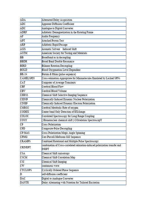
ADA Alternated Delay AcquisitionADC Apparent Diffusion CoefficientADC Analogue to Digital ConverterADRF Adiabatic Demagnetization in the Rotating FrameAF Audio FrequencyAPT Attached Proton TestARP Adiabatic Rapid PassageASIS Aromatic Solvent　Induced ShiftASTM American Society for Testing and MaterialsBB Broadband as in decouplingBBDR Broad Band Double ResonanceBIRD Bilinear Rotation DecouplingBOLD Blood Oxygenation Level DependentBR-24 Burum & Rhim (pulse sequence)CAMELSPIN Cross-relaxation Appropriate for Minimolecules Emulated by Locked SPNs CAT Computer of Average TransientsCBF Cerebral Blood FlowCBV Cerebral Blood VolumeCHESS Chemical Shift Selective Imaging SequenceCIDNP Chemically Induced Dynamic Nuclear PolarizationCINEP Chemically Induced Dynamic Electron PolarizationCMRO2 Cerebral Metabolic Rate of oxygenCODEX Center-band Only Detection of EXchangeCOLOC Correlated Spectroscopy for Long Range CouplingCOSY ( Homonuclear chemical shift ) COrrelation SpectroscopYCP Cross PolarizationCPD Composite-Pulse DecouplingCP/MAS Cross Polarization/Magic Angle SpinningCPMG Carr-Purcell-Meiboom Gill SequenceCRAMPS Combined Rotational and Multiple Pulse SpectroscopyCRINEPT combination of Cross-correlated relaxation-induced polarization transfer and INEPTCSA Chemical Shift AnisotropyCSCM Chemical Shift Correlation MapCSI Chemical Shift ImagingCW continuous waveCYCLOPS Cyclically Ordered Phase SequenceD self-diffusion coefficientDAC Digital to Analogue ConverterDANTE Delay Alternating with Nutation for Tailored ExcitationDAS Dynamic Angle SpinningDCNMR NMR in Presence of an Electric Direct CurrentDD Dipole-DipoleDECSY Double-quantum Echo Correlated SpectroscopyDEFT Driven Equilibrium Fourier TransformDEPT Distortionless Enhancement by Polarization TransferDFT Discrete Fourier Transform2DFTS two Dimensional FT SpectroscopyDIPSI Composite-pulse Decoupling in the presence of scalar Interactions DMF, DMF-d7 dimethyl-formamide, heptadeuterio-DMFDMSO, DMSO-d6 dimethyl-sulfoxide, hexadeuterio-DMSODNMR Dynamic NMRDNP Dynamic Nuclear PolarizationDOR Double-Orientation RotationDOSY Diffusion-Ordered SpectroscopyDOUBTFUL Double Quantum Transitions for Finding Unresolved Lines2D-PASS 2D-Phase Adjusted Spinning SidebandsDPFGSE Double Pulsed Field Gradient Spin EchoDQ(C) Double Quantum (Coherence)DQD Digital Quadrature DetectionDQF Double Quantum FilterDQF-COSY Double Quantum Filtered COSYDRDS Double Resonance Difference SpectroscopyDRESS Depth Resolved SpectroscopyDSA Data-Shift AcquisitionECOSY Exclusive Correlation SpectroscopyEFG Electric Field GradientELD Energy Level DiagramENDOR Electron-nuclear Double ResonanceENMR Electrophonetic NMREPI Echo Planar ImagingEPR Electron Paramagnetic ResonanceESR Electron Spin ResonanceEXORCYCLE 4-step phase cycle for spin echoesEXSY Exchange SpectroscopyFFT Fast Fourier TransformationFID Free Induction DecayFIREMAT FIve p Replicated Magic Angle TurningFLASH Fast Low-angle Shot imagingFLOPSY Flip-Flop SpectroscopyFMRI functional Magnetic Resonance ImagingFOCSY Foldover-Corrected SpectroscopyFONMR field FOcusing Nuclear Magnetic ResonanceFOV Field of ViewFSLG Frequency-Switched Lee-GoldburgFT Fourier TransformationGARP Globally Optimized Alternating Phase Rectangular PulseGES Gradient-Echo SpectroscopyGRASS Gradient-Recalled Acquisition in the Steady StateGRASP Gradient-Accelerated SpectroscopyGROPE Generalized compensation for Resonance Offset and Pulse length errors GS Gradient SpectroscopyH,C-COSY 1H,13C chemical-shift COrrelation SpectroscopYH,X-COSY 1H,X-nucleus chemical-shift COrrelation SpectroscopYHETCOR Heteronuclear Correlation SpectroscopyHMBC Heteronuclear Multiple-Bond CorrelationHMQC Heteronuclear Multiple Quantum CoherenceHOESY Heteronuclear Overhauser Effect SpectroscopyHOHAHA Homonuclear Hartmann-Hahn spectroscopyHR High ResolutionHSP Homogeneity-Spoiling PulseHSQC Heteronuclear Single Quantum CoherenceINADEQUATE Incredible Natural Abundance Double Quantum Transfer Experiment INDOR Internuclear Double ResonanceINEPT Insensitive Nuclei Enhanced by PolarizationINVERSE H,X correlation via 1H detectionIR Inversion-RecoveryISIS Image-Selected In vivo SpectroscopyJR Jump-and-Return sequence (90y-τ- 90- y)JRES J-resolved spectroscopyLAOCOON Least squares Adjustment Of Calculated On Observed NMR spectraLED longitudinal eddy-current delay pulse sequence for diffusion coefficient measurementLIS Lanthanide (chemical shift reagent ) Induced Shift LP Linear PredictionLSR Lanthanide Shift ReagentMAH Magic-Angle HoppingMARF Magic Angle in the Rotating FrameMAS Magic-Angle SpinningMASS Magic Angle Sample SpinningMAT Magic-Angle TurningMEM Maximum Entropy MethodMLEV M.Levitt's CPD sequenceMO Molecular Orbital (in quantum theory )MQ(C) Multiple-Quantum ( Coherence )MQF Multiple-Quantum FilterMQMAS Multiple-Quantum Magic-Angle SpinningMQS Multi Quantum SpectroscopyMRA Magnetic Resonance AngiographyMREV Mansfield-Rhim-Elleman-Vaughan sequence for dipolar line narrowing MRI Magnetic Resonance ImagingMRS Magnetic Resonance SpectroscopyNMR Nuclear Magnetic ResonanceNMRI Nuclear Magnetic Resonance ImagingNOE Nuclear Overhauser EffectNOESY Nuclear Overhauser Effect SpectroscopyNQCC Nuclear Quadrupole Coupling ConstantNQR Nuclear Quadrupole ResonanceNQS Non Quaternary SuppressionP2DSS Pseudo 2D Sideband SuppressionPENDANT Polarization Enhancement During Attached Nucleus TestingPFG Pulsed Field GradientPGSE Pulsed Gradient Spin Echo*PMFG Pulsed Magnetic Field GradientPHORMAT Phase CORrected MATppm Parts per millionPOF Product Operator FormalismPRFT Partially Relaxed Fourier TransformPSD Phase-sensitive DetectionPSF Point Spread FunctionPW Pulse WidthQPD Quadrature Phase DetectionQF Quadrupole moment/Field gradient(interaction or relaxation mechanism) RARE Rapid Acquisition Relaxation EnhancedRCT Relayed Coherence TransferRECSY Multistep Relayed Coherence SpectroscopyREDOR Rotational Echo Double ResonanceRELAY Relayed Correlation SpectroscopyRFDR Radio Frequency Driven DecouplingRF Radio FrequencyRIDE RIng Down EliminationROESY Rotating Frame Overhauser Effect SpectroscopyROTO ROESY-TOCSY RelayRR Rotational ResonanceSA Shielding AnisotropySC Scalar CouplingSDDS Spin Decoupling Difference SpectroscopySE Spin EchoSECSY Spin-Echo Correlated SpectroscopySEDOR Spin Echo Double ResonanceSEFT Spin-Echo Fourier Transform Spectroscopy (with J modulation) SELINCOR Selective Inverse CorrelationSELINQUATE Selective INADEQUATESEMQT Subspectral Editing using a Multiple-Quantum TrapSELTICS Sideband ELimination by Temporary Interruption of the Chemical Shift SFORD Single Frequency Off-Resonance DecouplingSI Spectroscopy ImagingSKEWSY Skewed Exchange SpectroscopySNR or S/N Signal-to-noise RatioSPACE Spatial and Chemical-Shift Encoded ExcitationSPI Selective Population InversionSPIRAL Spiral Echo Planar ImagingSPT Selective Population TransferSQF Single-Quantum FilterSR Saturation-RecoverySSFP Steady-State Free PrecisionSSI Solid State ImagingSTE Stimulated EchoSTEAM Stimulated Echo Acquisition Mode for imagingSTRAFI STRAy Field ImagingTANGO Testing for Adjacent Nuclei with a Gyration OperatorTCF Time Correlation FunctionTE Time delay between excitation and Echo maximumTEDOR Transferred Echo Double ResonanceTFA, TFA-d trifluoro-acetic acid ( CF3COOH ), deuterio-TFA ( CF3COOD ) TIGER Technique for Importing Greater Evolution ResolutionTMR Topical Magnetic ResonanceTMS tetramethylsilane, (CH3)4SiTOCSY Total Correlation SpectroscopyTOE Truncated NOETORO TOCSY-ROESY RelayTOSS Total Suppression of SidebandsTPPI Time-proportional Phase IncrementationTPPM Two-Pulse Phase ModulationTQ Triple QuantumTQF Triple-Quantum FilterTR Time for Repetition of excitationTROSY Transverse Relaxation-Optimized SpectroscopYUE Unpaired Electron (relaxation mechanism)VAS Variable Angle SpinningVOSY Volume-Selective SpectroscopyWAHUHA Waugh-Huber-Haeberlen SequenceWALTZ-16 A broadband decoupling sequenceWATERGATE Water suppression pulse sequenceWEFT Water Eliminated Fourier TransformXCORFE H,X correlation using a fixed evolution timeX-Filter Selection of 1H-1H correlations when both H are coupled to XX-Half-Filter Selection of 1H-1H correlations when one H is coupled to XZ-COSY COSY with z-filterZ-Filter pulse sandwich for elimination of signal components with dispersive phase ZECSY Zero-Quantum Echo-Correlated SpectroscopyZQ(C) Zero-Quantum (Coherence)ZQF Zero-Quantum Filterβ-COSY COSY with small flip angle mixing pulse βΨ-COSY pseudo-COSY using incremented freq.-selective excitationT1 Longitudinal (spin-lattice) relaxation time for MZT2 Transverse (spin-spin) relaxation time for MxyT1ρT1 of spin-locked magnetization in rotating frameT2ρT2 of spin-locked magnetization in rotating frametn time domain of the n-th dimensionFn frequency domain of the n-th dimensiontm mixing timeτc rotational correlation time。

Addendum

1.1 Stresses in the Target. Length of the Target Tooth
The analysis of results obtained by a Monte Carlo simulation of the proton beam transport to the NuMI target using mentioned above input conditions shows that: the proton beam is essentially non-symmetrical in the horizontal plane (X{direction); the beam distribution in the vertical plane (Y{direction) is symmetrical, but non{Gaussian and may be described well by the 8-th order polynomial N (y) = P4=0 k y2k . k Results of stress calculations in the target as functions of the tooth length are shown in Figure 1.1 for graphite target and in Figure 1.2 for beryllium one. As it follows from these Figures: for graphite target the equivalent stress reaches its minimum value of 16.3 MPa at the length of the tooth equal to 6.2 mm; for beryllium target the equivalent stress reaches its minimum value of 117 MPa at the length of the tooth equal to 8 mm.

核磁共振图谱解析解析NMR

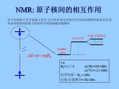
同核J-偶合(Homonuclear J-Coupling)
多重峰出现的规则: 1. 某一原子核与N个相邻的核相互偶合将给出(n+1)重峰. 2. 等价组合具有相同的共振频率.其强度与等价组合数有关. 3. 磁等价的核之间偶合作用不出现在谱图中. 4. 偶合具有相加性. 例如: observed spin coupled spin intensity
JCH JCH
H C
p-pulse on H
H C
这相当于使用一系列1800脉冲快速照射氢核。 pH pH
C-H
+J/2
C-H
-J/2
C-H
+J/2
pH
C-H
-J/2
pH
C-H
+J/2
pH
C-H
-J/2
Fig. 4-2.5 The proton-decoupled 13C spectrum of 1-propanol
H-12C H-13C H-13C x100
105 Hz
proton-coupled spectra (nondecoupled spectra)
Quartet, J=127 Hz
Proton-coupled spectra for large molecules are often difficult to interpret. The multiplets from different C commonly overlap because the 13C-H coupling constants are frequently larger than the chemical differences of the C in the spectrum. 原子核间的偶合导致谱图的复杂化(―精细裂分”)，灵敏度下降。 Fig. 4-2.4 Ethyl phenylacetate. (a) The proton-coupled 13C spectrum. (b) The proton-decoupled 13C spectrum

SL Note96–38(AP)Beam Size,Emittance and Optical Functions in LEPJohn M.Jowett22May1996AbstractThis note has a twofold purpose.Theﬁrst is to discuss the physical princi-ples behind the estimation of emittance from beam size using measuring devices(such as the BEUV monitors)in LEP.This includes an explanation of some of thediscrepancies between“measured emittances”and the luminosity in LEP.The second,closely related,purpose is more technical.The program MAD cal-culates a variety of functions describing the optics of LEP.The relation of beamsizes to emittance is used to illustrate the proper application of MAD’s capabili-ties and the meaning of the results.Some pitfalls in application of semi-intuitiverecipes are pointed out.Most of the plots in this note are better viewed in colour.The note is also avail-able on the World-Wide-Web at:Contents1Introduction2 2Calculations32.1The commands and32.2The command5 3Examples53.1An Imperfect LEP at82GeV63.2Effect of a more symmetric RF system163.3Perfect machine with symmetric RF20 4Conclusions231List of Figures1RF voltage distribution(imperfect ring)6 2Horizontal beam size(imperfect ring)7 3V ertical beam size(imperfect ring)7 4Horizontal-beating(imperfect ring)9 5V ertical-beating(imperfect ring)9 6Errors in horizontal beam size(imperfect ring)10 7Errors in vertical beam size(imperfect ring)11 8Horizontal dispersion(imperfect ring)12 9V ertical dispersion(imperfect ring)12 10Over-estimate of horizontal emittance(imperfect ring)13 11Over-estimate of vertical emittance(imperfect ring)13 12Beam tilt(imperfect ring)14 13Beam sizes at the IP(imperfect ring)15 14V ertical beam size(symmetric RF)16 15V ertical-beating(symmetric RF)17 16V ertical dispersion(symmetric RF)17 17Beam tilt(symmetric RF)18 18Over-estimate of vertical emittance(symmetric RF)18 19Beam sizes at the IP(symmetric RF)19 20Horizontal beam size(perfect ring)20 21V ertical-beating(perfect ring)21 22Horizontal dispersion(perfect ring)21 23Beam sizes at the IP(perfect ring)22 List of Tables1IntroductionThere are apparent inconsistencies between estimates of the LEP beam emittances from direct measurements via the BEUV monitors and the luminosity measured by the LEP experiments.While LEP ran at the Z-resonance,these were not a serious concern as the LEP experiments could measure luminosity rapidly and without any knowledge of the emittance.However the much smaller cross-sections at LEP2energies will make it harder to measure luminosity directly and there will be a greater reliance on construct-ing the beam sizes at the IPs from the measured emittances.As it has been shown that the discrepancies are unlikely to be instrumental[1],the current view is that the discrepancy arises from poor knowledge of the beam optics at the source point for the synchrotron light detected by the BEUV.In particular,it has been shown[2]that better agreement can be obtained by using measured-functions and including the linear focusing perturbations due to the beam-beam interactions.2In this note,I shall examine another aspect of the question,namely:is the usual description of the beam optics in terms of-and dispersion functions adequate to de-scribe the relation(1) between the emittance and beam size?Given the strong energy-sawtoothing effects at high energy,we might need to re-examine this relationship.In particular,we should review how we get the values of and and how much they depend on the(un-known)errors in the machine.It has also been shown,in simulation[3],that it is possible,at least in principle,to make the-functions correspond more approximately to their theoretical values by a matching procedure involving the strengths of the interaction region quadrupoles.This relies on the(generally valid)assumption that errors in these quadrupoles are the main source of“-beating”.This note contains no experimental data or discussion of the measurement device itself.It illustrates theoretical computations with numerical examples and examines the consequences of different ways of extracting the emittance from the beam size.How-ever these have a direct bearing on how measurements—even those performed with perfect instrumentation—are interpreted.Along the way,I have included a number of technical remarks footnotes which may be useful to people doing optics calculations for LEP at high energy.2CalculationsWithin MAD[4],there are various ways one might go about calculating the emittance and beam size.The following is intended as a review for non-specialists.It sketches the physical meaning of the various methods with a minimum of formalism.Optics afﬁcionados are encouraged to jump straight to Section3.2.1The commands andThe recommended way is to use the command to calculate the emittances and the command to calculate the beam sizes and correlation functions at selected points around the ring.Let me make it clear that,to the best of our present knowledge, these commands correctly include all physical effects determining the emittance and beam size in the context of linear single-particle dynamics including synchrotron radi-ation.I shall therefore use them as a reference and refer to the their results as the“true”beam sizes.“Errors”in other calculations of the beam size or emittance will be quoted with respect to these values.This note expands and supersedes,but does not invalidate,preliminary calculations shown at the LEP Studies Working Group meeting of30April1996.Those calculations used a crude method to gen-erate vertical emittance from betatron coupling.This note does it better.3If we could put a correct description of the real LEP into MAD,then we would want for nothing but these commands.Unfortunately,we do not know the imperfections ofthe real machine in sufﬁcient detail and this is where the complications set in.Afterﬁnding the closed orbit(ﬁxed point of the one-turn map from the starting az-imuth of the ring),MADﬁnds the eigenvectors of the tangent map and expresses themin terms of the primitive physical coordinates at the starting point of the ring[4].These eigenvectors deﬁne the three normal modes of linear particle motionabout the closed orbit.Integrals around the ring[5]of the mean radiation power andthe two-point correlation function of its deviation from the mean(quantumﬂuctuation)projected into these modes give the radiation damping and diffusion rate from quantumexcitation.These are combined to give the emittances of the normal modes.The beam emittances are just the average values of the action variables for each normal mode.The command expresses the total horizontal displacement at a given az-imuth,,say,in terms of the normal modes.It then averages over the distribution to compute the beam sizes from the emittances.Correlation functions such as give the degree of“coupling”between planes.The optics enters here through the magnitudes of the components of the eigenvec-tors.The relations in(1)can be viewed as a special case where the horizontal displace-ment only contains components from the radial“betatron”mode and the synchrotronoscillation mode.Atﬁrst sight,the MAD commands do not appear to furnish values of the dispersion functions.This is partly because they are not explicitly needed in the calculations of the beam sizes.In the literature,oneﬁnds many slightly different deﬁnitions of the dispersion functions.For present purposes,I propose to use a statistical deﬁnition(2)The momentum variable is the fractional deviation of the particle’s energy from a nominal value(usually given in units of in MAD).The same values can be de-rived from the generalised-functions printed out by MAD’s command which is based on the same physics as and.In the plots which follow,these dispersion functions will be labelled as“Dx(env)”or something similar,to reﬂect their derivation from the command.Since the three coordinates are given in units of metres,the quantity is just the bunch length.The command shows how it varies around the ring.Often reﬂecting the experience and temperament of the author.42.2The commandThis command is much deprecated and much used,both with good reason.In the past, its main use was to calculate the Courant-Snyder or“Twiss”functions(including the dispersion function),ignoring the effects of the RF and radiation.In the simplest version of the command,the transverse betatron coupling is also ignored.This com-mand remains of use as a guide to matching new optics(particularly for hadron rings) but you have to be careful what you do with it.In operational practice,the Twiss func-tions needed in various applications have been taken from a table computed once and for all for an ideal ring.Sometimes better results are obtained by using values measured by the“1000turns method”.If the RF cavities and radiation are switched on in MAD,then will calcu-late Twiss functions taking them into account.In this case,it is well-known that the -functions are good approximations to those calculated by but that the dis-persion functions are signiﬁcantly wrong.3ExamplesThe following subsections treat a variety of cases,all based on this year’s nominal physics optics at82GeV.The optics is set up using the MAD commands:Rather than give further detail here,let me say just say that you canﬁnd theﬁles I used in various sub-directories of:In each case,the optics and beam parameters are calculated for both positrons and elec-trons.The results of the various MAD commands are dumped out into tables and com-pared and analysed in a spreadsheet environment.For technical reasons,and because I want to make direct comparisons of,I show the values of optical functions at the beam position monitors(BPMs)and inter-action points,rather than at,say,the source points of the BEUV or other instruments.I used V ersion8.19/3of MAD.If they are“Twiss”-anything,they are most deﬁnitely functions and not“Twiss parameters”.To allow electrons to circulate in MAD,you have to reverse the sequence of machine elements(time-reversal)and reﬂect the machine in a mirror to reverse all the magneticﬁelds(but not the electricﬁelds). This is a consequence of a fundamental physical principle(non-CPT invariance when radiation is in-cluded).The BPMs and IPs are elements with zero length and have the agreeable property that,when the sequence is reversed,their entrances and exits are the same and they provide invariant observation points in all MAD commands.Indeed,some commands let you specify the centre or either end of an element as an observation point.However not all of the commands I needed to use for this study are so obliging.In fact,the only one which offers this feature plus the further convenience of the command is.is physically equivalent to.The command was introduced a few years ago precisely in order to allow observation points at the source points of instruments like the BEUV which lie inside magnets.53.1An Imperfect LEP at82GeVThis is an imperfect machine.I added random misalignments and tilts to dipoles,quad-rupoles and sextupoles to perturb the optics and generate a moderate amount of beta-tron coupling.After correcting the RMS horizontal and vertical orbits average orbits down to0.6mm and0.4mm respectively,the tune was corrected back to its nominal value using the main QF and QD strings.For further details of the magnitudes of the imperfections,please consult theﬁleThe RF distribution corresponds to the installation of cavities at the1996startupwithisratherFigure1:Imperfect ring:Distribution of RF voltage around the ring,computed as de-scribed in[7].The true horizontal and vertical beam sizes of the two beams are shown in Fig-ures2and3.The vertical beam sizes are signiﬁcantly different because of differences in the optical functions but mainly because the emittances of second normal mode forpositrons and electrons are different(and).These values correspond to emittance ratios of1.1%and0.6%,typical of a very good physicsﬁll.To be precise,the orbit was corrected with RF and radiation switched off.This corresponds fairly closely to what is done in operations,which is just as well as it is the only way to correct the orbit with the Micado algorithm,even inside MAD.This is based on an script describing the imperfections of LEP which has evolved over several years. With the improved element selection scheme in the latest version of MAD,it turned out to be necessary to rewrite the script quite substantially.600.511.522.533.5I P 1P U .Q D 22.R 1P U .Q D 40.L 2P U .Q S 10.L 2P U .Q S 8.R 2P U .Q D 36.R 2P U .Q D 26.L 3P U .Q L 2B .L 3P U .Q L 18.R 3P U .Q D 44.L 4P U .Q S 12.L 4P U .Q S 6.R 4P U .Q D 32.R 4P U .Q D 30.L 5P U .Q L 5.L 5P U .Q L 16.R 5P U .Q D 48.L 6P U .Q S 15.L 6P U .Q S 4.R 6P U .Q D 28.R 6P U .Q D 34.L 7P U .Q L 7.L 7P U .Q L 14.R 7P U .Q D 46.R 7P U .Q S 17.L 8P U .Q S 1A .R 8P U .Q D 24.R 8P U .Q D 38.L 1P U .Q L 9.L 1s i g x / m mFigure 2:Imperfect ring:The true horizontal beam size (command)at allthe BPMs and IPs around the ring for both e and e .0.050.10.150.20.250.30.350.40.45I P 1P U .Q D 22.R 1P U .Q D 40.L 2P U .Q S 10.L 2P U .Q S 8.R 2P U .Q D 36.R 2P U .Q D 26.L 3P U .Q L 2B .L 3P U .Q L 18.R 3P U .Q D 44.L 4P U .Q S 12.L 4P U .Q S 6.R 4P U .Q D 32.R 4P U .Q D 30.L 5P U .Q L 5.L 5P U .Q L 16.R 5P U .Q D 48.L 6P U .Q S 15.L 6P U .Q S 4.R 6P U .Q D 28.R 6P U .Q D 34.L 7P U .Q L 7.L 7P U .Q L 14.R 7P U .Q D 46.R 7P U .Q S 17.L 8P U .Q S 1A .R 8P U .Q D 24.R 8P U .Q D 38.L 1P U .Q L 9.L 1s i g y / m mFigure 3:Imperfect ring:The true vertical beam size (command)at all theBPMs and IPs around the ring for both e and e .7Figures4and5show the ratios of the-functions calculated with and without ra-diation.The“-beating due to radiation”is quite signiﬁcant in the vertical mode and different for the two beams.Figures6and7show the differences in beam sizes obtained by naive application of formulas like(1)with various versions of the optical functions.In each case a percent-age error relative to the true beam size is quoted.Except for the second case(where the dispersion function computed using the command with radiation is used), the results are reasonable in the horizontal plane.In the vertical plane the errors are large in all cases.Figure8shows that the statistical deﬁnition,(2),of the horizontal dispersion func-tion is in rather good agreement with the obtained from the command without radiation and RF.On the other hand,Figure9shows that the statistical dispersion in the vertical plane is about a factor of two larger in this example.Figures6and7showed the error obtained by mis-predicting the beam size from a knowledge of the emittances.It is perhaps more important to consider the process of estimating the emittance from knowledge of the beam sizes,e.g.,at a device like the BEUV.For this purpose we can imagine that there is a device measuring the beam size at every BPM or IP and invert(1)to estimate the emittance(assuming knowledge of the energy spread).Figures10and11shows the resulting error in the estimate of horizontal and vertical emittance.The error is very large in the vertical plane and could easily explain the observed discrepancy between the“measured vertical emittance”and the luminosity monitors.The main reason for the error in the naive calculation is the tilt of the beam proﬁles in conﬁguration space.This is characterised by the quantity(3) which satisﬁes.This quantity is plotted for the positrons in Figure12. Despite what would normally be considered a very small global“coupling”,this quan-tity can take on rather large values locally.The effect of this on the estimation of beam sizes at the IPs is shown(somewhat indirectly)in Figure13.Here the beam sizes at the IPs are reconstructed from knowl-edge of the true emittances in various ways.Although there is little scope for error in the horizontal plane,the estimates of vertical beam sizes can vary quite widely.If one takes into account that the vertical emittance being fed into such calculations could in practice be a factor of two or so larger than the true one,it is easy to see that the vertical beam size at the IPs could be over-estimated.This is not to deny the importance of other effects such as the perturbation of the optics by the beam-beam interaction.800.20.40.60.811.2I P 1P U .Q D 22.R 1P U .Q D 40.L 2P U .Q S 10.L 2P U .Q S 8.R 2P U .Q D 36.R 2P U .Q D 26.L 3P U .Q L 2B .L 3P U .Q L 18.R 3P U .Q D 44.L 4P U .Q S 12.L 4P U .Q S 6.R 4P U .Q D 32.R 4P U .Q D 30.L 5P U .Q L 5.L 5P U .Q L 16.R 5P U .Q D 48.L 6P U .Q S 15.L 6P U .Q S 4.R 6P U .Q D 28.R 6P U .Q D 34.L 7P U .Q L 7.L 7P U .Q L 14.R 7P U .Q D 46.R 7P U .Q S 17.L 8P U .Q S 1A .R 8P U .Q D 24.R 8P U .Q D 38.L 1P U .Q L 9.L 1b e t a x (r a d )/b e t a x (n o n -r a d )Figure 4:Imperfect ring:The ratio non-radfor both e and e .All calculationsinclude the same imperfections.0.20.40.60.811.21.4I P 1P U .Q D 22.R 1P U .Q D 40.L 2P U .Q S 10.L 2P U .Q S 8.R 2P U .Q D 36.R 2P U .Q D 26.L 3P U .Q L 2B .L 3P U .Q L 18.R 3P U .Q D 44.L 4P U .Q S 12.L 4P U .Q S 6.R 4P U .Q D 32.R 4P U .Q D 30.L 5P U .Q L 5.L 5P U .Q L 16.R 5P U .Q D 48.L 6P U .Q S 15.L 6P U .Q S 4.R 6P U .Q D 28.R 6P U .Q D 34.L 7P U .Q L 7.L 7P U .Q L 14.R 7P U .Q D 46.R 7P U .Q S 17.L 8P U .Q S 1A .R 8P U .Q D 24.R 8P U .Q D 38.L 1P U .Q L 9.L 1b e t a y (r a d )/b e t a y (n o n -r a d )Figure 5:Imperfect ring:The ratio radfor both e and e .All calculationsinclude the same imperfections.9electrons, radiating enveleNAME BETX DX sigx/mm BETX DX sigx/mm BETX DX sigx/mm IP141.66-0.02 1.07 1.06941.41-0.02 1.06284 1.0600542.71-0.02 1.0796 1.08049Figure 6:Imperfect ring:These plots show errors in various calculations of the hori-zontal beam size for both e and e ,starting from the (true)emittances and constructing the beam sizes according to (1)with various versions of the optical functions.The error is always quoted relative to the true beam sizes calculated by .10electrons, radiating enveleNAME BETY DY sigy/mm BETY DY sigy/mm BETY DY sigy/mm IP127.660.0090.0910.06925.020.010.08680.11243930.220.010.07060.09399Figure 7:Imperfect ring:These plots show errors in various calculations of the vertical beam size for both e and e ,starting from the (true)emittances and constructing the beam sizes according to (1)with various versions of the optical functions.The error is always quoted relative to the true beam sizes calculated by .11-20.00%-15.00%-10.00%-5.00%0.00%5.00%10.00%15.00%I P 1P U .Q D 30.R 1P U .Q D 24.L 2P U .Q S 1A .R 2P U .Q D 32.R 2P U .Q D 22.L 3P U .Q L 5.R 3P U .Q D 38.R 3P U .Q S 17.L 4P U .Q S 6.R 4P U .Q D 40.R 4P U .Q L 16.L 5P U .Q L 9.R 5P U .Q D 46.R 5P U .Q S 12.L 6P U .Q S 10.R 6P U .Q D 48.R 6P U .Q L 11.L 7P U .Q L 14.R 7P U .Q D 44.L 8P U .Q S 8.L 8P U .Q S 15.R 8P U .Q D 42.L 1P U .Q L 7.L 1Figure 10:Imperfect ring:The fraction by which the horizontal emittance is over-estimated at each BPM when the true beam size ()is converted to an emit-tance using optical functions calculated by the command without radiation,but with perfect knowledge of the imperfections,according to (1).0.00%20.00%40.00%60.00%80.00%100.00%120.00%140.00%I P 1P U .Q D 30.R 1P U .Q D 24.L 2P U .Q S 1A .R 2P U .Q D 32.R 2P U .Q D 22.L 3P U .Q L 5.R 3P U .Q D 38.R 3P U .Q S 17.L 4P U .Q S 6.R 4P U .Q D 40.R 4P U .Q L 16.L 5P U .Q L 9.R 5P U .Q D 46.R 5P U .Q S 12.L 6P U .Q S 10.R 6P U .Q D 48.R 6P U .Q L 11.L 7P U .Q L 14.R 7P U .Q D 44.L 8P U .Q S 8.L 8P U .Q S 15.R 8P U .Q D 42.L 1P U .Q L 7.L 1Figure 11:Imperfect ring:The fraction by which the vertical emittance is over-estimated at each BPM when the true beam size ()is converted to an emit-tance using optical functions calculated by the command without radiation,but with perfect knowledge of the imperfections,according to (1).13G:\HOME\JOWETT\LEP96\BEUVBEAT\SEED2\OPTICSIN.XLS[Beam sizes at IPs]23:25 2Exp / m 2.7E-08082GeV Exe / m 2.7E-08sigep0.00129000sigee0.00129Eyp / m3E-10Eye / m 1.7E-10mixed functions non-radiating sigx/mm positrons, radiating envpos electrons, radiating envele sigx / mmNAME BETX DX+ (non-ra- (non-rad)BETX DX sigx/mm BETX DX sigx/mm e+ (mixed)e- (mixed)IP2 2.352-0.00730.25350.25403 2.35-0.0070.253360.25331 2.327-0.0060.252010.252270.25335720.252626IP4 3.196-0.00020.29520.29587 3.1617E-040.293620.29366 3.228-0.0020.296720.297230.29362330.297373IP6 2.8720.00310.27990.28052 2.9090.0030.281710.28156 2.8320.00290.277930.278330.28171590.278547IP8 1.9370.00650.230.23051 2.0140.0040.234440.23388 1.870.00820.226080.226140.23452510.226489 non-radiating sigy/mm positrons, radiating envpos electrons, radiating envele sigy/mmNAME BETY DY+ (non-ra- (non-rad)BETY DY sigy/mm BETY DY sigy/mm e+ (mixed)e- (mixed)IP20.044-0.00020.00360.002710.042-1E-040.003540.004450.046-2E-040.002750.00370.00353710.002751IP40.048-0.00050.00380.002880.045-6E-040.003690.004590.053-4E-040.002960.003850.00369110.002962IP60.052-0.00070.0040.003060.049-9E-040.003840.004930.059-5E-040.003120.004130.0038380.003121IP80.0510.00010.00390.002910.048-8E-050.003790.004440.0560.00020.003040.00360.00379150.003035Figure13:Imperfect ring:A comparison of beam sizes at the IPs computed from the (true)emittances using the non-radiating beam sizes compared with the true beam sizes computed by the command(envpos,envele).V alues of the various optical functions at the IPs are also shown in tabular form.153.2Effect of a more symmetric RF systemIt might be suggested that some of the effects seen in the above example are related to the asymmetry of the RF voltage distribution [6].To see how much can be attributed to RF asymmetry,I repeated the same calculations with exactly the same machine imper-fections but with an RF system adjusted to provide equal voltage in each octant.This meant that certain superconducting RF units were given voltages much higher than they are capable of in reality.The total RF voltage was kept the same as in the example of Section 3.1.The analogous plot to Figure 1would show eight equal bars of height 222MV .Figure 14shows that symnmstrizing the RF does not get rid of the difference in vertical beam sizes.0.050.10.150.20.250.30.350.4I P 1P U .Q D 22.R 1P U .Q D 40.L 2P U .Q S 10.L 2P U .Q S 8.R 2P U .Q D 36.R 2P U .Q D 26.L 3P U .Q L 2B .L 3P U .Q L 18.R 3P U .Q D 44.L 4P U .Q S 12.L 4P U .Q S 6.R 4P U .Q D 32.R 4P U .Q D 30.L 5P U .Q L 5.L 5P U .Q L 16.R 5P U .Q D 48.L 6P U .Q S 15.L 6P U .Q S 4.R 6P U .Q D 28.R 6P U .Q D 34.L 7P U .Q L 7.L 7P U .Q L 14.R 7P U .Q D 46.R 7P U .Q S 17.L 8P U .Q S 1A .R 8P U .Q D 24.R 8P U .Q D 38.L 1P U .Q L 9.L 1s i g y / m mFigure 14:Imperfect ring with symmetric RF:The true vertical beam size (command)at all the BPMs and IPs around the ring for both e and e .Figure 15shows that it changes,but does not eliminate,the vertical “-beating due to radiation”.The analogues of Figures 4,5and 8(not shown here),are also similar.Figure 16,the analogue of Figure 9,shows that the difference between the statistical and vertical dispersions remains large.This leads to a an over-estimate of the vertical emittance,Figure 18,comparable to the case with asymmetric RF,Figure 11.Figure 12shows that the beam tilt is again the main source of the problem.Figure 19shows that the beam sizes at the IPs remain different,as in Figure 13,despite the symmetric RF.We can conclude that this is due to imperfections.It seems160.20.40.60.811.21.4I P 1P U .Q D 22.R 1P U .Q D 40.L 2P U .Q S 10.L 2P U .Q S 8.R 2P U .Q D 36.R 2P U .Q D 26.L 3P U .Q L 2B .L 3P U .Q L 18.R 3P U .Q D 44.L 4P U .Q S 12.L 4P U .Q S 6.R 4P U .Q D 32.R 4P U .Q D 30.L 5P U .Q L 5.L 5P U .Q L 16.R 5P U .Q D 48.L 6P U .Q S 15.L 6P U .Q S 4.R 6P U .Q D 28.R 6P U .Q D 34.L 7P U .Q L 7.L 7P U .Q L 14.R 7P U .Q D 46.R 7P U .Q S 17.L 8P U .Q S 1A .R 8P U .Q D 24.R 8P U .Q D 38.L 1P U .Q L 9.L 1b e t a y (r a d )/b e t a y (n o n -r a d )Figure 15:Imperfect ring with symmetric RF:The ratio radfor both e ande .All calculations include the same imperfections.-0.15-0.1-0.050.050.10.15I P 1P U .Q D 30.R 1P U .Q D 24.L 2P U .Q S 1A .R 2P U .Q D 32.R 2P U .Q D 22.L 3P U .Q L 5.R 3P U .Q D 38.R 3P U .Q S 17.L 4P U .Q S 6.R 4P U .Q D 40.R 4P U .Q L 16.L 5P U .Q L 9.R 5P U .Q D 46.R 5P U .Q S 12.L 6P U .Q S 10.R 6P U .Q D 48.R 6P U .Q L 11.L 7P U .Q L 14.R 7P U .Q D 44.L 8P U .Q S 8.L 8P U .Q S 15.R 8P U .Q D 42.L 1P U .Q L 7.L 1D y / mFigure 16:Imperfect ring with symmetric RF:V ertical dispersion function calcu-lated by the command without radiation compared with that derived from thecommand using (2).17-0.8-0.6-0.4-0.200.20.40.60.8I P 128.R 128.L 2S 0.L 224.R 232.L 32B .L 324.R 332.L 4S 3.L 420.R 436.L 5L 5.L 520.R 536.L 6S 5.L 617.R 640.L 7L 7.L 717.R 740.L 8S 7.L 815.R 844.L 1L 9.L1Figure 17:Imperfect ring with symmetric RF:The beam tilt for positrons computed by the command in MAD.-20.00%0.00%20.00%40.00%60.00%80.00%100.00%120.00%140.00%160.00%I P 1P U .Q D 30.R 1P U .Q D 24.L 2P U .Q S 1A .R 2P U .Q D 32.R 2P U .Q D 22.L 3P U .Q L 5.R 3P U .Q D 38.R 3P U .Q S 17.L 4P U .Q S 6.R 4P U .Q D 40.R 4P U .Q L 16.L 5P U .Q L 9.R 5P U .Q D 46.R 5P U .Q S 12.L 6P U .Q S 10.R 6P U .Q D 48.R 6P U .Q L 11.L 7P U .Q L 14.R 7P U .Q D 44.L 8P U .Q S 8.L 8P U .Q S 15.R 8P U .Q D 42.L 1P U .Q L 7.L 1Figure 18:Imperfect ring with symmetric RF:The fraction by which the vertical emit-tance is over-estimated at each BPM when the true beam size ()is converted to an emittance using optical functions calculated by the command without radi-ation,but with perfect knowledge of the imperfections,according to (1).18plausible that correction of the-beating due to imperfections(as in[3])would help to equalise the beam sizes and luminosity between IPs.G:\HOME\JOWETT\LEP96\BEUVBEAT\SEED2\OPTICSIN.XLS[Beam sizes at IPs]21:59 2Exp / m 2.7E-08082GeV Exe / m 2.7E-08sigep0.00129000sigee0.00129Eyp / m3E-10Eye / m 1.7E-10mixed functions non-radiating sigx/mm positrons, radiating envpos electrons, radiating envele sigx / mmNAME BETX DX+ (non-ra- (non-rad)BETX DX sigx/mm BETX DX sigx/mm e+ (mixed)e- (mixed)IP2 2.352-0.00730.25350.25403 2.35-0.0070.253360.25148 2.327-0.0060.252010.255530.25335720.252626IP4 3.196-0.00020.29520.29587 3.1617E-040.293620.29342 3.228-0.0020.296720.2970.29362330.297373IP6 2.8720.00310.27990.28052 2.9090.0030.281710.28271 2.8320.00290.277930.276010.28171590.278547IP8 1.9370.00650.230.23051 2.0140.0040.234440.23511 1.870.00820.226080.224780.23452510.226489 non-radiating sigy/mm positrons, radiating envpos electrons, radiating envele sigy/mmNAME BETY DY+ (non-ra- (non-rad)BETY DY sigy/mm BETY DY sigy/mm e+ (mixed)e- (mixed)IP20.044-0.00020.00360.002710.042-1E-040.003540.004180.046-2E-040.002750.003890.00353710.002751IP40.048-0.00050.00380.002880.045-6E-040.003690.004250.053-4E-040.002960.00390.00369110.002962IP60.052-0.00070.0040.003060.049-9E-040.003840.004670.059-5E-040.003120.004060.0038380.003121IP80.0510.00010.00390.002910.048-8E-050.003790.004290.0560.00020.003040.003550.00379150.003035Figure19:Imperfect ring with symmetric RF:A comparison of beam sizes at the IPs computed from the(true)emittances using the non-radiating beam sizes compared with the true beam sizes computed by the command(envpos,envele).V alues of the various optical functions at the IPs are also shown in tabular form.19。

AS物理考试

This document consists of 24 printed pages.IB10 11_9702_11/6RP© UCLES 2010[Turn over*4840008086*UNIVERSITY OF CAMBRIDGE INTERNATIONAL EXAMINATIONS General Certificate of EducationAdvanced Subsidiary Level and Advanced LevelPHYSICS 9702/11Paper 1 Multiple ChoiceOctober/November 20101 hourAdditional Materials: Multiple Choice Answer Sheet Soft clean eraserSoft pencil (type B or HB is recommended)READ THESE INSTRUCTIONS FIRSTWrite in soft pencil.Do not use staples, paper clips, highlighters, glue or correction fluid.Write your n ame, Cen tre n umber an d can didate n umber on the An swer Sheet in the spaces provided unless this has been done for you.There are forty questions on this paper. Answer all questions. For each question there are four possible answers A , B , C and D .Choose the one you consider correct and record your choice in soft pencil on the separate Answer Sheet.Read the instructions on the Answer Sheet very carefully.Each correct answer will score one mark. A mark will not be deducted for a wrong answer. Any working should be done in this booklet.Dataspeed of light in free space, c = 3.00 × 108m s–1= 4π× 10–7H m–1 permeability of free space, µpermittivity of free space, ε= 8.85 × 10–12F m–1elementary charge, e = 1.60 × 10–19Cthe Planck constant, h = 6.63 × 10–34J s unified atomic mass constant, u = 1.66 × 10–27kgrest mass of electron, m e = 9.11 × 10–31kgrest mass of proton, m p = 1.67 × 10–27kg molar gas constant, R = 8.31J K–1mol–1the Avogadro constant, N A = 6.02 × 1023mol–1 the Boltzmann constant, k = 1.38 × 10–23J K–1 gravitational constant, G = 6.67 × 10–11N m2kg–2 acceleration of free fall, g = 9.81m s–2© UCLES 2010 9702/11/O/N/10© UCLES 2010 9702/11/O/N/10[Turn overFormulaeuniformly accelerated motion, s = ut + 221atv 2 = u 2 + 2as work done on/by a gas, W = p ∆V gravitational potential, φ = – r Gm hydrostatic pressure, p = ρghpressure of an ideal gas, p = V Nm 31<c 2> simple harmonic motion, a = – ω 2x velocity of particle in s.h.m., v = v 0 cos ωtv = ± ω 220x x − electric potential, V =rQ 04επ capacitors in series, 1 / C = 1 / C 1 + 1 / C 2 + . . . capacitors in parallel, C = C 1 + C 2 + . . .energy of charged capacitor, W = QV 21resistors in series, R = R 1 + R 2 + . . . resistors in parallel, 1 / R = 1 / R 1 + 1 / R 2 + . . . alternating current/voltage, x = x 0 sin ωt radioactive decay, x = x 0 exp(–λt ) decay constant,λ = 210.693t1 A signal has a frequency of 2.0MHz.What is the period of the signal?A 2µsB 5µsC 200nsD 500ns2 A metal sphere of radius r is dropped into a tank of water. As it sinks at speed v, it experiences adrag force F given by F = kr v, where k is a constant.What are the S I base units of k?A kg m2s–1B kg m–2s–2C kg m–1s–1D kg m s–23Which physical quantity would result from a calculation in which a potential difference is multiplied by an electric charge?A electric currentB electric energyC electric field strengthD electric powerSpace for working© UCLES 2010 9702/11/O/N/10© UCLES 20109702/11/O/N/10[Turn over4 The angular deflection of the needle of an ammeter varies with the current passing through theammeter as shown in the graph.angular deflectioncurrentWhich diagram could represent the appearance of the scale on this meter?AB CD 0123456789123456789123456789123456789Space for working© UCLES 20109702/11/O/N/105 The diagram shows a cathode-ray oscilloscope (c.r.o.) being used to measure the rate of rotation of a flywheel.The flywheel has a small magnet M mounted on it. Each time the magnet passes the coil, a voltage pulse is generated, which is passed to the c.r.o. The display of the c.r.o. is 10 cm wide. The flywheel is rotating at a rate of about 3000 revolutions per minute.Which time-base setting will display clearly separate pulses on the screen? A 1 s cm –1 B 10 ms cm –1C 100 µs cm –1D 1 µs cm –1Space for working© UCLES 20109702/11/O/N/10[Turn over6 A fixed quantity x 0 is measured many times in an experiment that has experimental uncertainty. A graph is plotted to show the number n of times that a particular value x is obtained.Which graph could be obtained if the measurement of x 0 has a large systematic error but a small random error?AnBnSpace for working© UCLES 20109702/11/O/N/107 A ball is thrown horizontally in still air from the top of a very tall building. The ball is affected by air resistance.What happens to the horizontal and to the vertical components of the ball’s velocity?horizontal componentof velocity vertical componentof velocity A decreases to zero increases at a constant rate B decreases to zero increases to a constant value C remains constant increases at a constant rate Dremains constantincreases to a constant value8 The velocity-time graph below is for a stone thrown vertically up into the air. Air resistance isnegligible.The stone is thrown up at time zero.Area X represents a distance of 5 m. Area Y represents a distance of 3 m.What is the displacement of the stone from its initial position at time t ? A 2 m B 3 mC 5 mD 8 mSpace for working© UCLES 2010 9702/11/O/N/10[Turn over9 In order that a train can stop safely, it will always pass a signal showing a yellow light before it reaches a signal showing a red light. Drivers apply the brake at the yellow light and this results in a uniform deceleration to stop exactly at the red light.The distance between the red and yellow lights is x .What must be the minimum distance between the lights if the train speed is increased by 20 %, without changing the deceleration of the trains? A 1.20 xB 1.25 xC 1.44 xD 1.56 x10 The gravitational field strength on the surface of planet P is one tenth of that on the surface ofplanet Q.On the surface of P, a body has a mass of 1.0 kg and a weight of 1.0 N.What are the mass and weight of the same body on the surface of planet Q?mass on Q / kgweight on Q / NA 1.0 0.1B 1.0 10C 10 10 D10 10011 A body, initially at rest, explodes into two masses M 1 and M 2 that move apart with speeds v 1and v 2 respectively.What is the ratio 21v v?A21M M B12M C21M M D12M MSpace for working© UCLES 20109702/11/O/N/1012 Two experiments are carried out using two trolleys of equal mass. All moving parts of the trolleysare frictionless, as is the surface that the trolleys move over. In both experiments, trolley X moves towards trolley Y, which is initially stationary.After the collision in experiment 1, X is stationary and Y moves off to the right.After the collision in experiment 2, the trolleys join and move off together.What types of collision occur in these experiments?experiment 1experiment 2A elastic elasticB elastic inelasticC inelastic elastic Dinelastic inelastic13 A rigid L-shaped lever arm is pivoted at point P.2 NThree forces act on the lever arm, as shown in the diagram.What is the magnitude of the resultant moment of these forces about point P? A 15 N m B 20 N mC 35 N mD 75 N mSpace for workingFWhat is the magnitude of the torque on the body produced by these forces?A F dB F sC 2F dD 2F s15 A street lamp is fixed to a wall by a metal rod and a cable.wallWhich vector triangle represents the forces acting at point P?A BC D16 What is the internal energy of a system?A the amount of heat supplied to the systemB the energy of the atoms of the systemC the total kinetic energy of the systemD the total potential energy of the system17 A steam turbine is used to drive a generator. The input power to the turbine is P I and the outputpower P O . The power loss in the turbine is P L , as shown below.LWhat is the efficiency of the turbine? AOLP P BOP P ICI P P LD IP P OSpace for working18 The diagram shows a lift system in which the elevator (mass m 1) is partly counterbalanced by aheavy weight (mass m 2).2At what rate does the motor provide energy to the system when the elevator is rising at a steady speed v ? (g = acceleration of free fall) A 21m 1 v 2 B21(m 1 – m 2)v 2C m 1gvD (m 1 – m 2)gv19 The Mariana Trench in the Pacific Ocean has a depth of about 10 km.Assuming that sea water is incompressible and has a density of about 1020 kg m –3, what would be the approximate pressure at that depth? A 105 PaB 106 PaC107 PaD 108 PaSpace for working20 A student writes some statements about solids, liquids and gases.1 Solids are rigid because the molecules in a solid vibrate.2 Liquids flow because the molecules in a liquid are closer than in a gas.3 Gases are less dense than liquids because the molecules in a gas move randomly.Which statements are correct?A 1 onlyB 1 and 3 onlyC 2 and 3 onlyD none of the above21The graph shows how force depends on extension for a certain spring.10.08.06.04.02.00.0010********extension/mmWhat is the energy stored in the spring when the extension is 30mm?A 0.095JB 0.19JC 0.25JD 0.95JSpace for workingm length of metal X joined to a 1.0 m length of metal Y.The cross-sectional area of the wire is uniform.A load hung from the wire causes metal X to stretch by 1.5 mm and metal Y to stretch by 1.0 mm.The same load is then hung from a second wire of the same cross-section, consisting of 1.0 m of metal X and 3.0 m of metal Y.What is the total extension of this second wire? A 2.5 mm B 3.5 mmC 4.8 mmD 5.0 mmSpace for working23displacement / cm / s__Which statement is correct?A B The wave has an amplitude of 2 cm and must be transverse.C The wave has an amplitude of 4 cm and could be either transverse or longitudinal.D The wave has an amplitude of 4 cm and must be transverse.24 The diagram shows a vertical cross-section through a water wave moving from left to right.At which point is the water moving upwards with maximum speed?Space for working25 When pla ne-pola rised light of a mplitude a is pa ssed through a pola rising filter a s shown, theamplitude of the light emerging is a cos θ.θa cos polarising filterThe intensity of the initial beam is I .What is the intensity of the emerging light when θ is 60.0°? A 0.250 IB 0.500 IC 0.750 ID 0.866 I2612When a microphone is moved between X a nd Y, a dista nce of 1.5 m, six nodes a nd seven antinodes are detected.What is the wavelength of the sound? A 0.50 m B 0.43 mC 0.25 mD 0.21 mSpace for working27Which electroma gnetic wa ve would ca use the most significa nt diffra ction effect for a n a tomic lattice of spacing around 10–10m?A infra-redB microwaveC ultravioletD X-ray28An electron is in an electric field of strength 5 × 104V m–1. The field is the only influence on the electron.The mass and charge of an electron are known.Which quantity can be calculated without any more information?A the force on the electronB the momentum of the electronC the kinetic energy of the electronD the speed of the electronSpace for working29 Electrons a re a ccelera ted a nd then directed into the uniform electric field between two pa ra llelplates in a vacuum.What best describes the shape of the path followed by the electrons in the field?A a downwards curve along a line that is part of a circleB a downwards curve along a line that is not part of a circleC an upwards curve along a line that is part of a circleD an upwards curve along a line that is not part of a circle30 A cha rged pa rticle is in the electric field between two horizonta l meta l pla tes connected to asource of constant potential difference, as shown. There is a force F on the particle due to the electric field.The separation of the plates is doubled.What will be the new force on the particle? A4F B2F C F D 2FSpace for working31The current in the circuit shown is 4.8A.What is the direction of flow and the rate of flow of electrons through the resistor R?direction of flow rate of flowA X to Y 3.0 × 1019s–1B X to Y 6.0 × 1018s–1C Y to X 3.0 × 1019s–1D Y to X 6.0 × 1018s–1Space for working© UCLES 20109702/11/O/N/10[Turn over32 Which component has the I -V graph shown?IVA filament lampB light-dependent resistorC semiconductor diodeD thermistor33 A copper wire is cylindrical and has resistance R .What will be the resistance of a copper wire of twice the length and twice the radius?A4R B2R C R D 2R34 A rela y is required to opera te 800 m from its power supply. The power supply ha s negligibleinternal resistance. The relay requires 16.0 V and a current of 0.60 A to operate.A ca ble connects the rela y to the power supply a nd two of the wires in the ca ble a re used to supply power to the relay.The resistance of each of these wires is 0.0050 Ω per metre.What is the minimum output e.m.f. of the power supply?A 16.6 VB 18.4 VC 20.8 VD 29.3 VSpace for working© UCLES 20109702/11/O/N/1035 The diagram shows part of a circuit.What is the total resistance of the combination of the three resistors?A 320 ΩB 240 ΩC 190 ΩD 80 Ω36 The diagram shows an arrangement of resistors.10 Ω10 ΩWhat is the total electrical resistance between X and Y? A less than 1 ΩB between 1 Ω and 10 ΩC between 10 Ω and 30 ΩD 40 ΩSpace for working© UCLES 20109702/11/O/N/10[Turn over37 In the circuit below, P is a potentiometer of tota l resista nce 10 Ω a nd Q is a fixed resistor ofresista nce 10 Ω. The ba ttery ha s a n e.m.f. of 4.0 V a nd negligible interna l resista nce. The voltmeter has a very high resistance.The slider on the potentiometer is moved from X to Y a nd a gra ph of voltmeter rea ding V is plotted against slider position.Which graph would be obtained?XAslider positionY V 420XBslider positionY V 420XDslider positionYV 420XCslider positionY V 42Space for workingPerm ission to reproduce item s where third-party owned m aterial protected by copyright is included has been sought and cleared where possible. Every reasonable effort has been made by the publisher (UCLES) to trace copyright holders, but if any items requiring clearance have unwittingly been included, the publisher will be pleased to make amends at the earliest possible opportunity.University of Cambridge International Examinations is part of the Cambridge Assessment Group. Cambridge Assessment is the brand name of University of Cambridge Local Examinations Syndicate (UCLES), which is itself a department of the University of Cambridge.© UCLES 2010 9702/11/O/N/1038 Uranium-235 may be represented by the symbol U 23592.Which row shows the numbers of nucleons, protons and neutrons in a 23592U nucleus?nucleons protons neutrons A 92 235 143 B 143 92 235 C 235 92 143 D235 143 9239 When a magnesium nucleus Mg 2512 is hit by a gamma ray, a sodium nucleus Na 2411 is formed andanother particle is emitted.What are the nucleon number (mass number) and proton number (atomic number) of the other particle produced in this nuclear reaction?nucleon numberproton numberA 0 –1B 0 1C 1 –1 D1 140 Which nuclear equation shows the beta decay of a nucleus of argon (Ar) into potassium (K)?A Ar 4421 → K 4019 + He 42 B Ar 4020 → K 4019 + e 01 C Ar 4018 → K 4019 + e 01− DAr4019 → K 4019 + γ00Space for working。

9702_s06_qp_1

For which quantity is the magnitude a reasonable estimate? A B C D frequency of a radio wave mass of an atom 500 pHz 500 µg
the Young modulus of a metal 500 kPa wavelength of green light 500 nm
© UCLES 2006
9702/01/M/J/06
5 4 A light meter measures the intensity I of the light falling on it. Theory suggests that this varies as the inverse square of the distance d.
x = x 0 exp(–λt )
λ = 0.693 t1
2
critical density matter of the Universe, equation of continuity, Bernoulli equation (simplified), Stokes' law, Reynolds' number, drag force in turbulent flow,
1
2
3
4 time / s
5
What is the distance travelled by the object in this time? A 9 4m B 20 m C 50 m D 100 m
The diagram shows a velocity-time graph for a mass moving up and down on the end of a spring. Which point represents the velocity of the mass when at the lowest point of its motion?

物理竞赛-第三届泛珠三角物理奥林匹克竞赛

electromagnetic wave. (1 point)
(iv)
An electromagnetic wave
r E
=
E0 (xr0eik1z
+
yr0eik2z )e−iωt
is propagating
along the z-axis displacement is
irn D
a=nεa0nEiso0t(rεopx xirc0emike1dzi+umε.
mbyeDdriu=mε
0tεheEr
relatiron betrween the electric , so D and E are always pointing
in
the
same direction. Find the torque per volume on the medium exerted by the
in the slab.
一个厚度为 d，介电常数为ε 的大平板以速度 v 沿 X-方向运动。它的表面与 Y-轴垂直。Z-方向加有磁场 B。求平板两表面上的束缚电荷密度，以及平板中的电场。
Q.5 (10 points) 题 5（10 分）
The space between two concentric conductor spherical shells of radii R1 and R3 is filled with two types of media. The dielectric constant and the conductivity of medium-1 and medium-2 are ε1, σ1 and ε2, σ2, respectively. The voltage difference between the two shells is V0.

1、下载文档前请自行甄别文档内容的完整性，平台不提供额外的编辑、内容补充、找答案等附加服务。
2、"仅部分预览"的文档,不可在线预览部分如存在完整性等问题,可反馈申请退款(可完整预览的文档不适用该条件!)。
3、如文档侵犯您的权益，请联系客服反馈,我们会尽快为您处理(人工客服工作时间：9:00-18:30)。

arXiv:astro-ph/0612205v1 8 Dec 2006Onthemeasurementoftheproton-aircrosssectionusinglongitudinalshowerproﬁles

R.Ulricha,J.Bl¨umera,R.Engela,F.Sch¨usslera,M.UngeraaForschungszentrumKarlsruhe,Institutf¨urKernphysik,Germany

Inthispaper,wewilldiscusstheprospectsofdeducingtheproton-aircrosssectionfromﬂuorescencetelescopemeasurementsofextensiveairshowers.AsitisnotpossibletoobservethepointofﬁrstinteractionX1directly,otherobservablescloselylinkedtoX1mustbeinferredfromthelongitudinalproﬁles.Thisintroducesadependenceonthemodelsusedtodescribetheshowerdevelopment.ThemoststraightforwardcandidateforagoodcorrelationtoX1isthedepthofshowermaximumXmax.WewilldiscussthesensitivityofanXmax-basedanalysisonσp−air

andquantifythesystematicuncertaintiesarisingfromthemodeldependence,parametersofthereconstruction

methoditselfandapossiblenon-protoncontaminationoftheselectedshowersample.

1.IntroductionOneofthemostimportantparameterneededforinterpretationofairshowermeasurementsistheproton-aircrosssectionσp−air,whichisnotwellknownatcosmicrayenergies.Collidermea-surementsoftheproton-(anti)protoncrosssec-tionhavetobeextrapolatedoverawideenergyrangetobeusedinmodelsofnucleareﬀectstopredicttheproton-aircrosssectionatultrahighenergies.Ontheotherhand,itmightbepossi-bletomeasureσp−airbyanalyzingextensiveairshowers(EAS).ThepointofﬁrstinteractioninslantdepthX1followstheexponentialdistributiondP(X1)λp−air·e−X1/λp−air.(1)Thecrosssectionσp−airisrelatedtotheabsorp-tionlengthλp−airasλp−air=Mmean/σp−air,withMmeanbeingthemeanmassofatarget(air)par-ticle.Thedepthandcharacteristicsoftheﬁrstinter-actionoftheprimarycosmicrayparticlewithamoleculeoftheatmospheredeterminestoalargeextenttheresultingshowershape.Thisim-pliesstrongcorrelationsoftheﬁrstinteractionwithexperimentallyobservableparametersoftheshower.Severalairshowerexperimentshaveprovidedmeasuredvaluesofσp−airbyexploitingcorrela-tionsofX1withobservablesfoundbyusingairshowersimulations[1,2,3,4,5].Ofcourse,theseresultsdependstronglyontheusedsimulationsandespeciallyonthechosenhighenergyhadronicinteractionmodel[6,7].TheHiRescollaborationproposedanewtech-niquewhichappearedtobealmostindependentofthehadronicinteractionmodel[8].TheideaistodecomposethemeasureddistributionofshowermaximadP(Xmax)/dXmaxintothetwoindepen-dentdistributionsofX1and∆Xwith

Xmax=X1+∆X.(2)Usingtheintroduced∆XonecanexpresstheXmaxdistributionasfoldingintegral

P(Xmax)=󰀃∞0dX1P(X1)·P(∆X|X1)(3)oftheX1and∆Xdistributions,whereasintheHiRes[8]approachP(∆X|X1)=P(∆X)isused.Measuringσp−airmeanstodeconvolvetheXmaxdistributionusingaknown∆Xdistribu-tion.Thedistributionof∆Xneedstobeinferredfromsimulations.

2.SimulationstudyToinvestigatethedeconvolutiontechnique,wesimulatedsetsofproton-inducedshowersof10EeVusingCONEX[9]withthehighenergy

12RalfUlrichetal.-2 X / gcm∆6007008009001000110012001300probability-610-510-410-310-210 < 13 (n=53876)2/gcmfirst 0< X < 39 (n=70785)2/gcmfirst 13< X < 78 (n=52277)2/gcmfirst 39< X < 533 (n=38958)2/gcmfirst 78< X-2 X / gcm∆

600650700750800850900950100010501100

probability-610

-510

-410

-310

-210

QGSJET proton

SIBYLL protonNEXUS protonQGSJETETII proton

Figure1.Leftpanel:Dependenceofthe∆X-distributiononX1.Rightpanel:Interactionmodeldependenceof∆X-distribution.

interactionmodelsQGSJET01[10],SIBYLL2.1[11],NEXUS3[12],andQGSJETII.3[13].Inadditionhelium,CNOandgamma-rayprimariesweresimulatedwithQGSJET01.Eachsetofsim-ulationscontains200.000events.

3.Universalityof∆XdistributionOneoftheimportantconditionsfortheappli-cabilityofthemethodproposedin[8]istheX1-independenceofthe∆Xdistribution.Foragivenmodel,thisisindeedthecaseasshowninFig.1(left).TheuniversalityinX1hasbeenveriﬁedforprotonprimariesusingNEXUS3,SIBYLL2.1,QGSJETII.3,andQGSJET01at1EeVand10EeV.Thereforeonecanuse

P(∆X|X1)=P(∆X).(4)However,theresulting∆Xdistributionde-pendsstronglyonthehadronicinteractionmodelusedforshowersimulation(Fig.1,right).Themaximumofthe∆Xdistributionisshiftedbyupto60g/cm2andtheslopebeyondthemaximumchangesbyuptoafactorof1.36.Thisintroducesaprincipalmodeldependencetothedeconvolu-tiontechnique.Itcanbetriedtoreducethisde-pendencebyaddinganadditionaldegreeoffree-dom,Xshift,whichallowsthe∆Xdistributionto

shiftalongthexaxisP(∆X)→P(∆X+Xshift).(5)Itismuchmorediﬃculttoreducethemodel-dependenceoftheshapeofthe∆Xdistribution.Thiswillnotbediscussedinthispaperbutweshallshowtheimpactofthismodel-dependenceontheresultingσp−airreconstruction.

4.StudyofthedeconvolutionmethodForeachmodel,aMonteCarlodatasetof50.000eventswasgeneratedandanalyzedwiththe∆Xdistributionsfoundpreviously.Node-tectoreﬀectsareconsidered.Twofreeparameters(λp−airandXshift)areﬁttedusingχ2minimiza-tionand