数字图像处理matlab版源码(第八章)
数字图像处理实验报告完整版
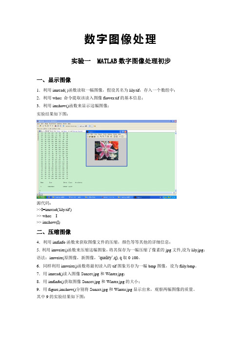
数字图像处理实验一 MATLAB数字图像处理初步一、显示图像1.利用imread( )函数读取一幅图像,假设其名为lily.tif,存入一个数组中;2.利用whos 命令提取该读入图像flower.tif的基本信息;3.利用imshow()函数来显示这幅图像;实验结果如下图:源代码:>>I=imread('lily.tif')>> whos I>> imshow(I)二、压缩图像4.利用imfinfo函数来获取图像文件的压缩,颜色等等其他的详细信息;5.利用imwrite()函数来压缩这幅图象,将其保存为一幅压缩了像素的jpg文件,设为lily.jpg;语法:imwrite(原图像,新图像,‘quality’,q), q取0-100。
6.同样利用imwrite()函数将最初读入的tif图象另存为一幅bmp图像,设为flily.bmp。
7.用imread()读入图像Sunset.jpg和Winter.jpg;8.用imfinfo()获取图像Sunset.jpg和Winter.jpg的大小;9.用figure,imshow()分别将Sunset.jpg和Winter.jpg显示出来,观察两幅图像的质量。
其中9的实验结果如下图:源代码:4~6(接上面两个) >>I=imread('lily.tif')>> imfinfo 'lily.tif';>> imwrite(I,'lily.jpg','quality',20);>> imwrite(I,'lily.bmp');7~9 >>I=imread('Sunset.jpg');>>J=imread('Winter.jpg')>>imfinfo 'Sunset.jpg'>> imfinfo 'Winter.jpg'>>figure(1),imshow('Sunset.jpg')>>figure(2),imshow('Winter.jpg')三、二值化图像10.用im2bw将一幅灰度图像转化为二值图像,并且用imshow显示出来观察图像的特征。
[数字图像处理](一)彩色图像转灰度图像的三种方式与效果分析
彩色图像转灰度图像的三种方式与效果分析](https://img.taocdn.com/s3/m/a9ad791dbb1aa8114431b90d6c85ec3a87c28bdb.png)
[数字图像处理](⼀)彩⾊图像转灰度图像的三种⽅式与效果分析图像处理(⼀)彩⾊图⽚转灰度图⽚三种实现⽅式最⼤值法imMax=max(im(i,j,1),im(i,j,2),im(i,j,3))平均法imEva=im(i,j,1)3+im(i,j,2)3+im(i,j,3)3加权平均值法imKeyEva=0.2989×im(i,j,1)+0.5870×im(i,j,2)+0.1140×im(i,j,3)matlba实现clc;close all;clear all;% 相对路径读⼊图⽚(和代码在同⼀⽂件夹下)im = imread('p2.jpg');%---查看图⽚,检测是否成功读⼊% 对显⽰的图⽚进⾏排版subplot(2,3,4);imshow(im);% 对图⽚进⾏命名title('原图');[col,row,color] = size(im);%col为图⽚的⾏数,row为图⽚的列数,color对于彩⾊图⽚⼀般为3,每层对应RGB %利⽤matlab⾃带的函数进⾏ rgb_to_gray;im_matlab = rgb2gray(im);subplot(2,3,1);imshow(im_matlab);title('matlab⾃带rgb2gray');%--------------------------------------------------------%---⽤最⼤值法% 创建⼀个全为1的矩阵,长宽等同于原图的im_max = ones(col,row);for i = 1:1:colfor j = 1:1:rowim_max(i,j) = max( im(i,j,:) );endend% 将矩阵变为8byte⽆符号整型变量(不然⽆法显⽰图⽚)% 最好在计算操作结束后再变化,不然会有精度问题!!im_max = uint8(im_max);subplot(2,3,2);imshow(im_max);title('最⼤值法');%--------------------------------------------------------% 平均值法im_eva = ones(col,row);for i = 1:1:colfor j = 1:1:rowim_eva(i,j) = im(i,j,1)/3 + im(i,j,2)/3 + im(i,j,3)/3 ;% 两种的结果其实⼀样,但是如果先转换为uint8就会出现精度问题%sum1 = im(i,j,1)/3 + im(i,j,2)/3 + im(i,j,3)/3%sum2 = ( im(i,j,1) + im(i,j,2)+ im(i,j,3) )/3;%fprintf( " %.4f %.4f \n",sum1 ,sum2 ) ;endendim_eva = uint8(im_max);subplot(2,3,3);imshow(im_eva);title('平均值法');%--------------------------------------------------------% 加权平均法(rgb2gray所使⽤的权值)im_keyeva = ones(col,row);% 加权算法先转换为uint8计算效果更好im_keyeva = uint8(im_max);for i = 1:1:colfor j = 1:1:rowim_keyeva(i,j) = 0.2989*im(i,j,1) + 0.5870*im(i,j,2) + 0.1140*im(i,j,3) ;endendsubplot(2,3,5);imshow(im_keyeva);title('加权平均法');Processing math: 100%附matlab——rgb2gray源码function I = rgb2gray(X)%RGB2GRAY Convert RGB image or colormap to grayscale.% RGB2GRAY converts RGB images to grayscale by eliminating the% hue and saturation information while retaining the% luminance.%% I = RGB2GRAY(RGB) converts the truecolor image RGB to the% grayscale intensity image I.%% NEWMAP = RGB2GRAY(MAP) returns a grayscale colormap% equivalent to MAP.%% Class Support% -------------% If the input is an RGB image, it can be of any numeric type. The output% image I has the same class as the input image. If the input is a% colormap, the input and output colormaps are both of class double.%% Notes% -----% RGB2GRAY converts RGB values to grayscale values by forming a weighted % sum of the R, G, and B components:%% 0.2989 * R + 0.5870 * G + 0.1140 * B%% The coefficients used to calculate grayscale values in RGB2GRAY are% identical to those used to calculate luminance (E'y) in% Rec.ITU-R BT.601-7 after rounding to 3 decimal places.%% Rec.ITU-R BT.601-7 calculates E'y using the following formula:%% 0.299 * R + 0.587 * G + 0.114 * B%% Example% -------% I = imread('example.tif');%% J = rgb2gray(I);% figure, imshow(I), figure, imshow(J);%% indImage = load('clown');% gmap = rgb2gray(indImage.map);% figure, imshow(indImage.X,indImage.map), figure, imshow(indImage.X,gmap);%% See also RGB2IND, RGB2LIGHTNESS.% Copyright 1992-2020 The MathWorks, Inc.narginchk(1,1);isRGB = parse_inputs(X);if isRGBI = matlab.images.internal.rgb2gray(X);else% Color map% Calculate transformation matrixT = inv([1.0 0.956 0.621; 1.0 -0.272 -0.647; 1.0 -1.106 1.703]);coef = T(1,:);I = X * coef';I = min(max(I,0),1);I = repmat(I, [1 3]);end%--------------------------------------------------------------------------function is3D = parse_inputs(X)is3D = (ndims(X) == 3);if is3D% RGBif (size(X,3) ~= 3)error(message('MATLAB:images:rgb2gray:invalidInputSizeRGB'))end% RGB can be single, double, int8, uint8,% int16, uint16, int32, uint32, int64 or uint64validateattributes(X, {'numeric'}, {}, mfilename, 'RGB');elseif ismatrix(X)% MAPif (size(X,2) ~= 3 || size(X,1) < 1)error(message('MATLAB:images:rgb2gray:invalidSizeForColormap'))end% MAP must be doubleif ~isa(X,'double')error(message('MATLAB:images:rgb2gray:notAValidColormap'))endelseerror(message('MATLAB:images:rgb2gray:invalidInputSize'))end总结通过上⾯的代码结合实际的测试,果然,matlab⾃带的rgb2gray也就是加权平均的⽅法,对光线明暗的处理是最好的。
基于matlab对图像进行高通、低通、带通滤波

数字图像处理三级项目—高通、低通、带通滤波器摘要在图像处理的过程中,消除图像的噪声干扰是一个非常重要的问题。
利用matlab软件,采用频域滤波的方式,对图像进行低通和高通滤波处理。
低通滤波是要保留图像中的低频分量而除去高频分量,由于图像中的边缘和噪声都对应图像傅里叶频谱中的高频部分,所以低通滤波可以除去或消弱噪声的影响并模糊边缘轮廓;高通滤波是要保留图像中的高频分量而除去低频分量,所以高通滤波可以保留较多的边缘轮廓信息。
低通滤波器有巴特沃斯滤波器和高斯滤波器等等,本次设计使用的低通滤波器为****。
高通滤波器有巴特沃斯滤波器、高斯滤波器、Laplacian高通滤波器以及Unmask高通滤波器等等,本次设计使用巴特沃斯高通滤波器。
1、频域低通滤波器:设计低通滤波器包括 butterworth and Gaussian (选择合适的半径,计算功率谱比),平滑测试图像test1和2。
实验原理分析根据卷积定理,两个空间函数的卷积可以通过计算两个傅立叶变换函数的乘积的逆变换得到,如果f(x, y)和h(x, y)分别代表图像与空间滤波器,F(u, v)和H(u, v)分别为响应的傅立叶变换(H(u, v)又称为传递函数),那么我们可以利用卷积定理来进行频域滤波。
在频域空间,图像的信息表现为不同频率分量的组合。
如果能让某个范围内的分量或某些频率的分量受到抑制,而让其他分量不受影响,就可以改变输出图的频率分布,达到不同的增强目的。
频域空间的增强方法的步骤:(1)将图像从图像空间转换到频域空间;(2)在频域空间对图像进行增强;(3)将增强后的图像再从频域空间转换到图像空间。
低通滤波是要保留图像中的低频分量而除去高频分量。
图像中的边缘和噪声都对应图像傅里叶频谱中的高频部分,所以低通滤波可以除去或消弱噪声的影响并模糊边缘轮廓。
理想低通滤波器具有传递函数:其中D0为制定的非负数,D(u,v)为点(u,v)到滤波器中心的距离。
傅里叶变换简单应用
像傅里叶函数频谱图
8
fftshift %快速傅里叶变换后的图像
平移函数
五·总结
1
对于傅里叶变换,它能够应用到许多的领域,不仅仅是在图像处理方面。
2
通过这次自己动手进行对傅里叶变换应用的动手实验,能够更好地将傅里叶变换应用到实 际生活中,不再是仅仅只会做题。更加的理解了傅里叶变换在实际应用中的作用和用法。
3
傅里叶变换能够更好地运用到实践当中,我们还应该不断的学习,去更加的完善傅里叶变 换在实际中的应用。
20XX
Thanks! 谢谢观看!
单击此处添加正文,文字是您思想的提炼,为了演示发布的良好效果,请言简 意赅地阐述您的观点。
析。
二·步骤流程图
流程图: 对得到的实验结果进行检查,分析。
打开 MATL AB
更改默认路径, 将实验所需文
件放入
编写实验程序, 将程序保存到
默认文件夹
运行程序,检 查错误并纠正, 得到实验结果
三·MATLAB程序源代码: (一)对原图像进行傅里叶
变换
(二)输出彩色图像的傅里叶频谱
(三)对彩色图像进行二维DCT变换
一·用MATLAB实现步骤
1
打开计算机,安装和启动MATL AB程
2
设置默认路径为C盘下的图片文件夹,
序。
将实验所需材料放入该文件夹内。
3
利用MATL AB工具箱中的函数编制
FFT频谱显示的函数。
4
调入、显示获得的图像,图像储存格
式应为“.jpg”。
5
对该程序进行编译,检查错误并纠正。 6
ቤተ መጻሕፍቲ ባይዱ
运行,并显示结果,比较差异进行分
利 用 计 算 机 上 安 装 的 M AT L A B 软 件 , 我 们 可 以 编 写 程 序 代 码 来用傅里叶变换对数字图像进行处理。
基于MatLab的数字图像清晰化方法
直方图的分布,使得直方图移向暗区,可以看出图像的视觉效
·62·
Computer Era No. 4 2008
基于 Web 的授课质量评价系统的研究与实践
刘利俊 1,吴达胜 2 (1. 杭州广播电视大学网络中心,浙江 杭州 310012;2. 浙江林学院信息工程学院)
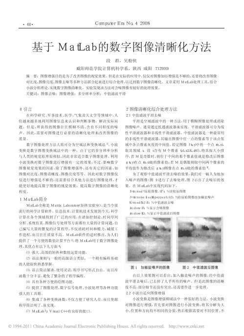
g1 和 g2 分别为门限阈值(g1<g2)。当噪声较小时,它对小波
系数的增益较大;当噪声较大时,对小波系数的增益较小。该算
法达到了自适应增强的效果。在 MatLab 中使用自适应阈值增
强方法的代码如下。
[x,ma p]=imre a d‘( 中值滤波后图像.tif’); %读取原图像
x=double (x);
直方图均衡化是较好的直方图修正方法,它生成了自适应 的变换函数,它是以已知图像的直方图为基础的。然而,一旦一 幅图像的变换函数计算完毕,它将不再改动,除非直方图有变 动。直方图均衡化通过扩展输入图像的灰度级到较宽亮度尺度 的范围来实现图像的增强,但这种方法并不总能得到成功的结 果。在 MatLab 中使用如下代码实现直方图匹配增强对比度,相 应的图像与图像直方图示于图 5 及图 6。
指标体系的适应性原则。 系统运行的性能和分布与集中处理。由于整个学校学生
人数众多,同时用户可能会很多,有时也许会多达几千个,因 而系统运行的性能是非常关键的,系统应该具有分布与集中 处理功能。
系统的安全性。为了尽量避免报复现象的产生,系统的安 全保密工作应该规定不同的用户具有不同的操作权限。系统用 户可以分成四个群体:学生、教师、领导、专家。安全性问题主要 考虑以下几点:①学生群体只能对当前任课教师进行评价;② 教师群体只能看到他人(学生、同时、领导、专家)对自己的评价 结果,而看不到具体的评价者情况,以免教师对他人实行报复; 同时教师可以对同行进行评价,这些同行必须是与评价者在同 一 学 院(系)的 ,否 则 代 表 性 不 强 ;③ 领 导 群 体 只 能 对 本 学 院 (系)教师进行评价;④专家群体可以评价学校的全体教师。同 时系统还要能够对一些不负责任的学生进行监督控制,需要设 置专门的超级用户可查看学生对教师的评价细节(包括学生学 号、姓名、班级、评价分数等信息)。
数字图像处理课程设计报告matlab
数字图像处理课程设计报告姓名:学号:班级: .net设计题目:图像处理教师:赵哲老师提交日期: 12月29日一、设计内容:主题:《图像处理》详细说明:对图像进行处理(简单滤镜,模糊,锐化,高斯模糊等),对图像进行处理(上下对称,左右对称,单双色显示,亮暗程度调整等),对图像进行特效处理(反色,实色混合,色彩平衡,浮雕效果,素描效果,雾化效果等),二、涉及知识内容:1、二值化2、各种滤波3、算法等三、设计流程图四、实例分析及截图效果:运行效果截图:第一步:读取原图,并显示close all;clear;clc;% 清楚工作窗口clc 清空变量clear 关闭打开的窗口close allI=imread('1.jpg');% 插入图片1.jpg 赋给Iimshow(I);% 输出图II1=rgb2gray(I);%图片变灰度图figure%新建窗口subplot(321);% 3行2列第一幅图imhist(I1);%输出图片title('原图直方图');%图片名称一,图像处理模糊H=fspecial('motion',40);%% 滤波算子模糊程度40 motion运动q=imfilter(I,H,'replicate');%imfilter实现线性空间滤波函数,I图经过H滤波处理,replicate反复复制q1=rgb2gray(q);imhist(q1);title('模糊图直方图');二,图像处理锐化H=fspecial('unsharp');%锐化滤波算子,unsharp不清晰的qq=imfilter(I,H,'replicate');qq1=rgb2gray(qq);imhist(qq1);title('锐化图直方图');三,图像处理浮雕(来源网络)%浮雕图l=imread('1.jpg');f0=rgb2gray(l);%变灰度图f1=imnoise(f0,'speckle',0.01);%高斯噪声加入密度为0.01的高斯乘性噪声 imnoise噪声污染图像函数 speckle斑点f1=im2double(f1);%把图像数据类型转换为双精度浮点类型h3=1/9.*[1 1 1;1 1 1;1 1 1];%采用h3对图像f2进行卷积滤波f4=conv2(f1,h3,'same');%进行sobel滤波h2=fspecial('sobel');g3=filter2(h2,f1,'same');%卷积和多项式相乘 same相同的k=mat2gray(g3);% 实现图像矩阵的归一化操作四,图像处理素描(来源网络)f=imread('1.jpg');[VG,A,PPG] = colorgrad(f);ppg = im2uint8(PPG);ppgf = 255 - ppg;[M,N] = size(ppgf);T=200;ppgf1 = zeros(M,N);for ii = 1:Mfor jj = 1:Nif ppgf(ii,jj)<Tppgf1(ii,jj)=0;elseppgf1(ii,jj)=235/(255-T)*(ppgf(ii,jj)-T);endendendppgf1 = uint8(ppgf1);H=fspecial('unsharp');Motionblur=imfilter(ppgf1,H,'replicate');figure;imshow(ppgf1);调用function [VG, A, PPG] = colorgrad(f, T)if (ndims(f)~=3) || (size(f,3)~=3)error('Input image must be RGB');endsh = fspecial('sobel');sv = sh';Rx = imfilter(double(f(:,:,1)), sh, 'replicate');Ry = imfilter(double(f(:,:,1)), sv, 'replicate');Gx = imfilter(double(f(:,:,2)), sh, 'replicate');Gy = imfilter(double(f(:,:,2)), sv, 'replicate');Bx = imfilter(double(f(:,:,3)), sh, 'replicate');By = imfilter(double(f(:,:,3)), sv, 'replicate');gxx = Rx.^2 + Gx.^2 + Bx.^2;gyy = Ry.^2 + Gy.^2 + By.^2;gxy = Rx.*Ry + Gx.*Gy + Bx.*By;A = 0.5*(atan(2*gxy./(gxx-gyy+eps)));G1 = 0.5*((gxx+gyy) + (gxx-gyy).*cos(2*A) + 2*gxy.*sin(2*A));A = A + pi/2;G2 = 0.5*((gxx+gyy) + (gxx-gyy).*cos(2*A) + 2*gxy.*sin(2*A)); G1 = G1.^0.5;G2 = G2.^0.5;VG = mat2gray(max(G1, G2));RG = sqrt(Rx.^2 + Ry.^2);GG = sqrt(Gx.^2 + Gy.^2);BG = sqrt(Bx.^2 + By.^2);PPG = mat2gray(RG + GG + BG);if nargin ==2VG = (VG>T).*VG;PPG = (PPG>T).*PPG;endf1=rgb2gray(f);imhist(f1);title('素描图直方图');五,图像处理实色混合(来源网络)%实色混合I(I<=127)=0; %对像素进行处理,若值小于等于127,置0 I(I>127)=255; %对像素进行处理,若值大于127,置255 imshow(I);title('像素图');I1=rgb2gray(f);imhist(I1);title('像素图直方图');六,图像处理反色图f=imread('1.jpg');q=255-q;imshow(q);title('反色图');imhist(q1);title('反色图直方图');七,图像处理上下对称A=imread('1.jpg');B=A;[a,b,c]=size(A);a1=floor(a/2); b1=floor(b/2); c1=floor(c/2);B(1:a1,1:b,1:c)=A(a:-1:a-a1+1,1:b,1:c);figureimshow(B)title('上下对称');A=rgb2gray(A);figureimhist(A)title('上下对称直方图');八,图像处理类左右对称C=imread('1.jpg');A=C;C(1:a,1:b1,1:c)=A(1:a,b:-1:b+1-b1,1:c);figureimshow(C)title('左右对称');A=rgb2gray(A);figureimhist(A);title('左右对称直方图');九,图像处理单双色显示a=imread('1.jpg');a1=a(:,:,1);a2=a(:,:,2); a3=a(:,:,3);aa=rgb2gray(a);a4=cat(3,a1,aa,aa); a5=cat(3,a1,a2,aa);figuresubplot(121);imshow(a4);title('单色显示');subplot(122);imshow(a5);title('双色显示');a4=rgb2gray(a4);a5=rgb2gray(a5);figuresubplot(121);imhist(a4);title('单色显示直方图');subplot(122);imhist(a5);title('双色显示直方图');十,图像处理亮暗度调整a=imread('1.jpg');a1=0.8*a;figuresubplot(121);imshow(a1);title('暗图');subplot(122);imshow(a2);title('亮图')q3=rgb2gray(a1);q4=rgb2gray(a2);figuresubplot(121);mhist(q3);title('暗图直方图') subplot(122);imhist(q4);title('亮图直方图')十一,图像处理雾化处理q=imread('1.jpg');m=size(q,1);n=size(q,2);r=q(:,:,1);g=q(:,:,2);b=q(:,:,3);for i=2:m-10for j=2:n-10k=rand(1)*10;%产生一个随机数作为半径di=i+round(mod(k,33));%得到随机横坐标dj=j+round(mod(k,33));%得到随机纵坐标r(i,j)=r(di,dj);%将原像素点用随机像素点代替 g(i,j)=g(di,dj);b(i,j)=b(di,dj);endenda(:,:,1)=r;a(:,:,2)=g;a(:,:,3)=b;imshow(a)title('雾化处理图');q=rgb2gray(a);figureimhist(q);title('雾化处理图直方图');十二,图像处理高斯滤波I = imread('1.jpg');G =fspecial('gaussian', [5 5], 2);% fspecial生成一个高斯滤波器Ig =imfilter(I,G,'same');%imfilter使用该滤波器处理图片imshow(Ig);title('高斯滤波');I1=rgb2gray(Ig);imhist(I1);title('高斯滤波直方图');十三,图像处理色彩平衡(来自网络)im=imread('1.jpg');im2=im;%存储元图像im1=rgb2ycbcr(im);%将im RGB图像转换为YCbCr空间。
数字图像处理第二章 MATLAB中图象工具箱及图象.

1.2图像显示
1.getimage函数 格式 A=GETIMAGE(H). 返回图形句柄对象 H 中
包含的第一个图像的数据.H既可以是一条曲线, 图像 , 或纹理表面 .A 等同为图像的数据。格式 [X,Y,A]=GETIMAGE(H). 返 回 图 像 的 Xdata 到 X,Ydata到Y,Xdata和Ydata是表明x轴和y轴的范 围的两元素向量。 格式 […,A,FLAG]=GETIMAGE(H) 。返回指示 图像类型的整数型标记.FLAG可为下列值:
格式 IMAGE(RGB). 用于显示真彩色图像。
格式 IMAGE(X,MAP). 显示索引图 X 及其
调色板MAP。 格式 IMSHOW(FILENAME). 显示存储于 图形文件FILENAME中的图像。 H=IMSHOW(…).返回图像对象的句柄。
5.SUBIMAGE函数
格式SUBIMAGE(X,MAP).用来显示当前坐标中
2.imwrite函数 该函数用于把图像写入图形文件中。格式
IMWRITE(A,FILENAME,FMT)把图像A写入文 件FILENAME中。FILENAME指明文件名, FMT指明文件格式。A既可以是一个灰度图,也 可以是一个真彩图像。格式 IMWRITE(X,MAP,FILENAME,FMT)把索引图 及其调色板写入FILENAME中。MAP必须为合 法的MATLAB调色板,大多数图像格式不支持 多于256色的调色板。FMT的可能取值为tif或 tiff,jpg或jpeg,bmp,png,hdf,pcx,xwd。
0 不是图像,A返回一个空矩阵。 1 索引图。 2 标准灰度图。 3非标准灰度图。 4 RGB图像。 例如在用 imshow 直接从文件中显示一个
MATLAB在图像处理中的应用(2)

ห้องสมุดไป่ตู้
1引言
MATI。AB是一种基于向量(数组)而不是标量 的高级程序语言,因而MATLAB从本质上提供了 对图像的支持。从图像的数字化过程可以看出,数 字图像实际上就是一组有序的离散数据,使用 MATLAB可以对这些离散数据形成的矩阵进行一 次性的处理。因此,MATLAB是图像处理研究中 快速实现研究新构思的非常有用的工具。MAT— LAB推出了功能强大的适应于图像分析和处理的 工具箱,常用的有图像处理工具箱、小波工具箱及数 字信号处理工具箱。利用如此多的工具,我们可以 方便地从各个方面对图像的性质进行深入的研究。 本文从实际应用的角度介绍了如何利用MATLAB 进行图像的分析和处理。
图像变换技术是图像处理的重要工具,常应用 于图像压缩、滤波、编码和后续的特征抽取或信息分 析过程。MATLAB提供了常用的变换函数,如 filt2()与ifft2()函数分别实现二维快速傅立叶变换 及其逆变换,dot2()与idct2()函数实现离散余弦变 换及其逆变换,Randon(0与iradon()函数实现Ra- don变换与逆Radon变换。 3.5图像的边缘检测与图像分割
边缘检测是一种重要的区域处理方法,边缘是 所要提取目标和背景的分界线,提取出边缘才能将
目标和背景区分开来。MATL蛆中提供了基本的
~些边缘检测函数,如Sobel、Robert、Canny等等。 另外还提供了分水岭(water—shed)分割方法以及
基于区域的一些分割方法。另外还提供了大量的二 值数学形态学的函数,如腐蚀、膨胀、开操作、闭操作
■●I
- 1、下载文档前请自行甄别文档内容的完整性,平台不提供额外的编辑、内容补充、找答案等附加服务。
- 2、"仅部分预览"的文档,不可在线预览部分如存在完整性等问题,可反馈申请退款(可完整预览的文档不适用该条件!)。
- 3、如文档侵犯您的权益,请联系客服反馈,我们会尽快为您处理(人工客服工作时间:9:00-18:30)。
covmatrix.mfunction [C, m] = covmatrix(X)%COVMATRIX Computes the covariance matrix of a vector population.% [C, M] = COVMATRIX(X) computes the covariance matrix C and the % mean vector M of a vector population organized as the rows of% matrix X. C is of size N-by-N and M is of size N-by-1, where N is% the dimension of the vectors (the number of columns of X).% Copyright 2002-2004 R. C. Gonzalez, R. E. Woods, & S. L. Eddins% Digital Image Processing Using MATLAB, Prentice-Hall, 2004% $Revision: 1.4 $ $Date: 2003/05/19 12:09:06 $[K, n] = size(X);X = double(X);if n == 1 % Handle special case.C = 0;m = X;else% Compute an unbiased estimate of m.m = sum(X, 1)/K;% Subtract the mean from each row of X.X = X - m(ones(K, 1), :);% Compute an unbiased estimate of C. Note that the product is% X'*X because the vectors are rows of X.C = (X'*X)/(K - 1);m = m'; % Convert to a column vector.endfrdescp.mfunction z = frdescp(s)%FRDESCP Computes Fourier descriptors.% Z = FRDESCP(S) computes the Fourier descriptors of S, which is an % np-by-2 sequence of image coordinates describing a boundary.%% Due to symmetry considerations when working with inverse Fourier % descriptors based on fewer than np terms, the number of points in % S when computing the descriptors must be even. If the number of % points is odd, FRDESCP duplicates the end point and adds it at% the end of the sequence. If a different treatment is desired, the% sequence must be processed externally so that it has an even% number of points.%% See function IFRDESCP for computing the inverse descriptors.% Copyright 2002-2004 R. C. Gonzalez, R. E. Woods, & S. L. Eddins % Digital Image Processing Using MATLAB, Prentice-Hall, 2004% $Revision: 1.4 $ $Date: 2003/10/26 23:13:28 $% Preliminaries[np, nc] = size(s);if nc ~= 2error('S must be of size np-by-2.');endif np/2 ~= round(np/2);s(end + 1, :) = s(end, :);np = np + 1;end% Create an alternating sequence of 1s and -1s for use in centering% the transform.x = 0:(np - 1);m = ((-1) .^ x)';% Multiply the input sequence by alternating 1s and -1s to% center the transform.s(:, 1) = m .* s(:, 1);s(:, 2) = m .* s(:, 2);% Convert coordinates to complex numbers.s = s(:, 1) + i*s(:, 2);% Compute the descriptors.z = fft(s);ifrdescp.mfunction s = ifrdescp(z, nd)%IFRDESCP Computes inverse Fourier descriptors.% S = IFRDESCP(Z, ND) computes the inverse Fourier descriptors of % of Z, which is a sequence of Fourier descriptor obtained, for% example, by using function FRDESCP. ND is the number of% descriptors used to computing the inverse; ND must be an even % integer no greater than length(Z). If ND is omitted, it defaults % to length(Z). The output, S, is a length(Z)-by-2 matrix containing % the coordinates of a closed boundary.% Copyright 2002-2004 R. C. Gonzalez, R. E. Woods, & S. L. Eddins % Digital Image Processing Using MATLAB, Prentice-Hall, 2004% $Revision: 1.6 $ $Date: 2004/11/04 22:32:04 $% Preliminaries.np = length(z);% Check inputs.if nargin == 1 | nd > npnd = np;end% Create an alternating sequence of 1s and -1s for use in centering% the transform.x = 0:(np - 1);m = ((-1) .^ x)';% Use only nd descriptors in the inverse. Since the% descriptors are centered, (np - nd)/2 terms from each end of% the sequence are set to 0.d = round((np - nd)/2); % Round in case nd is odd.z(1:d) = 0;z(np - d + 1:np) = 0;% Compute the inverse and convert back to coordinates.zz = ifft(z);s(:, 1) = real(zz);s(:, 2) = imag(zz);% Multiply by alternating 1 and -1s to undo the earlier% centering.s(:, 1) = m.*s(:, 1);s(:, 2) = m.*s(:, 2);function P = princomp(X, q)%PRINCOMP Obtain principal-component vectors and related quantities. % P = PRINCOMP(X, Q) Computes the principal-component vectors of % the vector population contained in the rows of X, a matrix of% size K-by-n where K is the number of vectors and n is their% dimensionality. Q, with values in the range [0, n], is the number% of eigenvectors used in constructing the principal-components% transformation matrix. P is a structure with the following% fields:%% P.Y K-by-Q matrix whose columns are the principal-% component vectors.% P.A Q-by-n principal components transformation matrix% whose rows are the Q eigenvectors of Cx corresponding % to the Q largest eigenvalues.% P.X K-by-n matrix whose rows are the vectors reconstructed % from the principal-component vectors. P.X and P.Y are% identical if Q = n.% P.ems The mean square error incurred in using only the Q% eigenvectors corresponding to the largest% eigenvalues. P.ems is 0 if Q = n.% P.Cx The n-by-n covariance matrix of the population in X.% P.mx The n-by-1 mean vector of the population in X.% P.Cy The Q-by-Q covariance matrix of the population in% Y. The main diagonal contains the eigenvalues (in% descending order) corresponding to the Q eigenvectors.% Copyright 2002-2004 R. C. Gonzalez, R. E. Woods, & S. L. Eddins% Digital Image Processing Using MATLAB, Prentice-Hall, 2004% $Revision: 1.4 $ $Date: 2003/10/26 23:16:16 $[K, n] = size(X);X = double(X);% Obtain the mean vector and covariance matrix of the vectors in X. [P.Cx, P.mx] = covmatrix(X);P.mx = P.mx'; % Convert mean vector to a row vector.% Obtain the eigenvectors and corresponding eigenvalues of Cx. The% eigenvectors are the columns of n-by-n matrix V. D is an n-by-n% diagonal matrix whose elements along the main diagonal are the% eigenvalues corresponding to the eigenvectors in V, so that X*V =% D*V.[V, D] = eig(P.Cx);Princomp.m% Sort the eigenvalues in decreasing order. Rearrange the% eigenvectors to match.d = diag(D);[d, idx] = sort(d);d = flipud(d);idx = flipud(idx);D = diag(d);V = V(:, idx);% Now form the q rows of A from first q columns of V.P.A = V(:, 1:q)';% Compute the principal component vectors.Mx = repmat(P.mx, K, 1); % M-by-n matrix. Each row = P.mx. P.Y = P.A*(X - Mx)'; % q-by-K matrix.% Obtain the reconstructed vectors.P.X = (P.A'*P.Y)' + Mx;% Convert P.Y to K-by-q array and P.mx to n-by-1 vector.P.Y = P.Y';P.mx = P.mx';% The mean square error is given by the sum of all the% eigenvalues minus the sum of the q largest eigenvalues.d = diag(D);P.ems = sum(d(q + 1:end));% Covariance matrix of the Y's:P.Cy = P.A*P.Cx*P.A';。