Research on Measurements for Temperature and Stress of Pistons in Internal Combustion Engine
Establishment_of_Unstable_Flow_Model_and_Well_Test

M. Sazid et al.Stress Measurement with Rheological Stress Recovery Method and Its Application.Mathematical Problems in Engineering, 2016, Article ID: 7059151.https:///10.1155/2016/7059151[46]Jaeger, N.G.W.C.J.C. and Zimmerman, R.W. (2007) Fundamentals of Rock Me-chanics. 4th Edition, Wiley-Blackwell, Hoboken.[47]Gowida, A., Elkatatny, S. and Gamal, H. (2021) Unconfined Compressive Strength(UCS) Prediction in Real-Time While Drilling Using Artificial Intelligence Tools.Neural Computing and Applications, 33, 8043-8054.https:///10.1007/s00521-020-05546-7[48]Al Dhaif, R., Ibrahim, A.F. and Elkatatny, S. (2022) Prediction of Surface Oil Ratesfor Volatile Oil and Gas Condensate Reservoirs Using Artificial Intelligence Tech-niques. Journal of Energy Resources Technology, Transactions of the ASME, 144,Article 033001.https:///10.1115/1.4051298[49]Fang, X., Feng, H., Wang, Y. and Fan, T. (2022) Prediction Method and Distribu-tion Characteristics of in Situ Stress Based on Borehole Deformation—A Case Studyof Coal Measure Stratum in Shizhuang Block, Qinshui Basin. Frontiers in EarthScience (Lausanne), 10, 1-36.https:///10.3389/feart.2022.961311[50]Lin, H., et al. (2022) An Investigation of Machine Learning Techniques to EstimateMinimum Horizontal Stress Magnitude from Borehole Breakout. InternationalJournal of Mining Science and Technology, 32, 1021-1029.https:///10.1016/j.ijmst.2022.06.005[51]Abreu, R., Mejia, C. and Roehl, D. (2022) Inverse Analysis of Hydraulic FracturingTests Based on Artificial Intelligence Techniques. International Journal for Numer-ical and Analytical Methods in Geomechanics, 46, 2582-2602.https:///10.1002/nag.3419[52]Ibrahim, A.F., Gowida, A., Ali, A. and Elkatatny, S. (2021) Machine Learning Ap-plication to Predict In-Situ Stresses from Logging Data. Scientific Reports,11,Ar-ticle No. 23445.https:///10.1038/s41598-021-02959-9[53]Lawal, A.I. and Kwon, S. (2021) Application of Artificial Intelligence to Rock Me-chanics: A n Overview. Journal of Rock Mechanics and Geotechnical Engineering,13, 248-266.https:///10.1016/j.jrmge.2020.05.010World Journal of Engineering and Technology, 2023, 11, 273-280https:///journal/wjetISSN Online: 2331-4249ISSN Print: 2331-4222Establishment of Unstable Flow Model and Well Testing Analysis for Viscoelastic Polymer FloodingZheng Lv, Meinan WangBohai Oilfield Research Institute of CNOOC Ltd., Tianjin Branch, Tianjin, ChinaAbstractAt present, the polymer solution is usually assumed to be Newtonian fluid orpseudoplastic fluid, and its elasticity is not considered on the study of poly-mer flooding well testing model. A large number of experiments have shownthat polymer solutions have viscoelasticity, and disregarding the elasticity willcause certain errors in the analysis of polymer solution seepage law. Based onthe percolation theory, this paper describes the polymer flooding mechanismfrom the two aspects of viscous effect and elastic effect, the mathematicalmodel of oil water two-phase three components unsteady flow in viscoelasticpolymer flooding was established, and solved by finite difference method, andthe well-test curve was drawn to analyze the rule of well test curve in polymerflooding. The results show that, the degree of upward warping in the radialflow section of the pressure recovery curve when considering polymer elastic-ity is greater than the curve which not considering polymer elasticity. The re-laxation time, power-law index, polymer injection concentration mainly af-fect the radial flow stage of the well testing curve. The relaxation time, pow-er-law index, polymer injection concentration and other polymer floodingparameters mainly affect the radial flow stage of the well testing curve. Thelarger the polymer flooding parameters, the greater the degree of upwarpingof the radial flow derivative curve. This model has important reference signi-ficance for well-testing research in polymer flooding oilfields.KeywordsPolymer Flooding, Viscoelasticity, Well Testing, Mathematical Model,Seepage Law1. IntroductionPolymer flooding is an important way to improve oil recovery in production oil-How to cite this paper: Lv, Z. and Wang,M.N. (2023) Establishment of UnstableFlow Model and Well Testing Analysis forViscoelastic Polymer Flooding. World Jour-nal of Engineering and Technology, 11,273-280.https:///10.4236/wjet.2023.112019Received: April 6, 2023Accepted: May 6, 2023Published: May 9, 2023Copyright © 2023 by author(s) andScientific Research Publishing Inc.This work is licensed under the CreativeCommons Attribution InternationalLicense (CC BY 4.0)./licenses/by/4.0/Open AccessZ. Lv, M. N. Wangfields. It has been widely industrialized in China and has achieved good applica-tion results and economic benefits [1] [2] [3] [4] [5]. Most experts have con-ducted a lot of research on the percolation characteristics of polymer in porous media and its impact on oil displacement effect. However, in most analysis of polymer flooding percolation laws, people usually assume that polymer solution is Newtonian fluid or pseudoplastic fluid, without considering its elasticity. A large number of experiments have shown that polymer solutions have viscoelas-ticity, and disregarding their elasticity will cause certain errors in the analysis of polymer solution seepage law [6] [7] [8] [9] [10]. This article studies the rheo-logical and viscoelastic properties of polymer solution, provides a characteriza-tion method for the elastic viscosity of polymer solutions, and proposes a new polymer flooding well testing model which takes into account the viscoelastic properties of polymer, which guiding the study of percolation law in polymer flooding Oilfields.2. Mathematical Description for the Main Oil Displacement Mechanism of PolymerUnder certain temperature condition, the viscosity of polymer solution increases significantly with increasing concentration. Under static condition, the viscosity of the polymer solution can be expressed as the following equation.()023p w 1p 2p 3p 1A c A c A c µµ=++++ (1)In which, 0p µ is zero shear viscosity of polymer solution, Pa·s; μw is water viscosity, Pa·s; c p is Polymer solution concentration, mg/L; A 1, A 2, A 3 is coeffi-cient.Due to the generally low concentration of polymer solutions, 33pA c and its subsequent terms are often overlooked.()02p w 1p 2p 1A c A c µµ=++ (2)Using the Kerry model to describe the viscoelasticity of polymer solution.()()()1220eff pppf 1n µµµµθγ−∞∞ =+−+⋅(3)In which, μeff is viscoelastic polymer viscosity, Pa·s; pµ∞is ultimate shear rate viscosity, Pa·s; θf is relaxation time, s; n is power-law index.3. Establishment and Solution of a Mathematical Model for Oil-Water Two-Phase Flow in Polymer FloodingAssuming that polymer flooding is an isothermal displacement process and mul-tiphase flow satisfies the generalized Darcy’s law, the fluid consists of oil-water two-phase flow, with only oil components in the oil phase and water and polymer components in the water phase. Ignoring the influence of capillary pressure and gravity, the continuity equation of oil-water two-phase flow can be expressed as the following equations.()o ro o o o o o K K p q S t ρρφµ ⋅∂∇⋅∇+= ∂(4)Z. Lv, M. N. Wang()w rw w w w w eff KK p q S t ρρφµ ∂∇⋅∇+= ∂(5)()rw p w w p w p eff KK c p q c S c t φµ ∂∇⋅∇+= ∂(6)In which, ρo is oil phase density, kg/m 3; ρw is water phase density, kg/m 3; K is absolute permeability, m 2; K ro is oil relative permeability; K rw is water relative permeability; µo is oil phase viscosity, Pa·s; p o is oil phase pressure, Pa; p w is water phase pressure, Pa; ϕ is porosity; q o is oil recovery intensity, m 3/(s·m 3); q w is water injection intensity, m 3/(s·m 3); S o is oil saturation; S w is water saturation.From Equations (4) and (5), the pressure differential equations for the oil and water phases can be obtained as the following equations.o o o o o o ox oy wx wy w w o o o to w wp p p p x x y y x x y y p C q q t ρρλλλλρρρφρρ∂∂∂∂∂∂∂∂⋅+⋅+⋅+⋅ ∂∂∂∂∂∂∂∂∂−−∂ (7)o o wx wy ww o o w w w f w w w p p q x x y y S p p S C S C t t tλλφρρφφρ∂∂ ∂∂⋅+⋅+ ∂∂∂∂∂∂∂=++∂∂∂ (8) Under the condition of uniform grid, the oil phase pressure Equation (7), the water phase saturation seepage Equation (8), and the polymer component con-centration Equation (6) are respectively processed by finite difference, and the fi-nite difference model corresponding to the oil-water two-phase seepage mathe-matical model can be established.11111,o ,1,o 1,,o ,,o 1,,o ,1,n n n n n i j i j i j i j i j i j i j i j i j i j i j c p a p e p b p d p f +++++−−++++++=(9) ()()()111111w ,1,o ,11,o 1,1,o ,1,o 1,1,o ,1w ,w w w w f o w ,,w n n n n n n n i ji ji j i j i j i j i j i j i j i j i j i jnnni ji j t Scpa p e pb pd p V q tS C C p S φρφρρφ++++++−−++∆=++++∆ ++++ (10) ()()()111111p ,2,o ,12,o 1,2,o ,2,o 1,2,o ,1w ,1w p ,w ,w ,p ,p ,f o p ,,w w ,,nn n n n n n i j i ji j i j i j i j i j i j i j i j i j i jn n n nn i j i j i jn n ni ji j i jni ji ji jt c cp a p e p b p d p S V q c tS S c c C p c S V Sφφ++++++−−+++∆=++++∆− +−++(11)The coefficients in the above equation can be expressed as the following equa-tions.o,11o w w 22i j xi xi a TT ρρ−−=+; o ,11o w w 22i j xi xi b T T ρρ++=+; o ,11o w w 22i j yi yi c T T ρρ−−=+; o,11o w w 22i j yi yi d TT ρρ++=+; ()o t ,,,,,,i j i j i j i j i j i j n C V e a b c d t φρ =−++++ ∆;Z. Lv, M. N. Wang()o t ,o,w ,o ,,w i j n i ji j i j i j n C V f q V q V p t φρρρ=−−−∆; 1,1w 2i j xi a T −=; 1,1w 2i j xi b T+=; 1,1w 2i j yi c T−=; 1,1w 2i j yi d T+=;()w w w f ,1,1,1,1,1,i ji ji j i j i j i j nS C C V e a b c d tφρ + =−−−−−∆; 2,1w 2i jxi a T −=; 2,1w 2i j xi b T +=; 2,1w 2i j yi c T −=; 2,1w 2i j yi d T +=;w p f ,1,1,1,1,1,n i j i j i j i j i j i j n S c C V e a b c d t φ =−−−−−∆; 1o 21o 122j xi xi i i y h T x x λ±±±∆=∆+∆; 1o 21oy 122i yj j j j x h Ty y λ±±±∆=∆+∆; 1w 21w 122j xi xi i i y h Tx x λ±±±∆=∆+∆; 1w 21wy 122i yj j j j x h Ty y λ±±±∆=∆+∆;,i j i j V x y h =∆∆; o ro o o KK ρλµ=; w rww effKK ρλµ=; rw p p eff KK c λµ=The finite difference method is used to solve the problem, and the IMPES me-thod is used to solve the pressure implicitly, the saturation explicitly, and the po-lymer concentration explicitly. The solution process is as follows: Firstly, startingfrom the initial conditions, the pressure value at time n can be obtained from the pressure equation. A fter obtaining the pressure at each time step, the obtained node pressure is substituted into the saturation equation to obtain the water sa-turation value of each node at time n. Then, the water saturation value is substi-tuted into the polymer seepage equation to obtain the polymer concentration value of each node at time n. In this way, the reservoir pressure, oil saturation, water saturation, and polymer concentration values at different time steps can be obtained. Record the bottom hole pressure values at different times and the pres-sure values at any point in the formation, draw a well testing curve, and analyze the curve.4. Analysis of Polymer Flooding Well Testing CurveAfter the text edit has been completed, the paper is ready for the template. Dup-licate the template file by using the Save As command, and use the naming con-vention prescribed by your journal for the name of your paper. In this newly created file, highlight all of the contents and import your prepared text file. You are now ready to style your paper. The viscoelastic polymer flooding mathemat-ical model of the inverse five point method well pattern has been established, the basic parameter variables being are as follow, C t = 5.2 × 10⁻⁴ MPa −1, ϕ = 0.3, n = 0.4, K = 0.375 μm 2, c p = 2.0 × 10³ mg/L, p e = 20 MPa, h = 10 m, S wi = 0.4. The shut-in pressure recovery test curve of the central polymer injection well was drawn.The comparison of pressure dynamic curves between water flooding and po-lymer flooding is shown in Figure 1.Before polymer injection, the radial flow section of the water drive derivative curve is basically horizontal, and the recovery speed is stable. After polymer in-Z. Lv, M. N. Wangjection, a hump appears in the radial flow stage of the curve, and the pressure and pressure conductivity values are higher than those of water drive. The de-gree of warping in the radial flow section of the well testing curve when consi-dering polymer elasticity is greater than the curve which not considering poly-mer elasticity. A fter polymer injection, the viscosity of the displacement fluid increases, and the flow resistance within the formation increases, resulting in an upward trend in the radial flow section of the curve compared to water flooding. Compared with water flooding, polymer flooding has a higher viscosity of the displacement fluid, greater resistance to fluid flow in the formation, and higher injection pressure required. Therefore, the pressure and pressure derivative val-ues of polymer flooding well testing curves are higher than those of water flood-ing. Considering the elasticity of the polymer, in addition to shear viscosity, elas-tic viscosity is also taken into account. As the viscosity of the polymer increases, the flow resistance increases, resulting in a greater degree of upward warping in the radial flow section.The polymer flooding oil-water two-phase well test curves corresponding to different relaxation times are shown in Figure 2.Z. Lv, M. N. WangRelaxation time is a physical quantity that measures the elasticity of a polymersolution. From the graph, it can be seen that the relaxation time mainly affectsthe transition section and radial flow section of the well testing curve. The largerthe relaxation time, the greater the pressure and pressure derivative values. Thehigher the “hump” of the transition section and radial flow section, and thegreater the degree of upward warping of the radial flow section. Due to the con-sideration of the elastic viscosity of the polymer solution, the relaxation time af-fects the elastic viscosity of the polymer. As the relaxation time increases, the in-fluence of elasticity on the well testing curve gradually increases; The larger therelaxation time, the greater the elastic viscosity at the same shear rate, the greaterthe apparent viscosity, and the greater the seepage resistance of the fluid duringthe seepage process, resulting in a greater degree of upward warping of the radialflow section.The analysis curve of the influence factors of power law index on polymerflooding oil-water two-phase well testing is shown in Figure 3.The power-law index is a parameter to characterize the non-newtonian prop-erty of polymer solution, and the power-law index of Newtonian fluid is 1. Thepower-law index mainly affects the degree of upwarping in the radial flow sec-tion. The closer the power-law index is to 1, the higher the pressure and pressurederivative curve, and the greater the degree of upwarping in the radial flow sec-tion of the pressure derivative curve. Near the injection well, the closer the pow-er law index is to 1, the weaker the non-newtonian property of the polymer solu-tion is, the lower the shear thinning degree is at the same shear rate, the higherthe viscosity of the polymer solution is, the greater the seepage resistance is, andsistance, and the greater the degree of upward warping in the radial flow section; The higher the viscosity of the polymer, the smaller the range of influence dur-ing the same production time, and the shorter the radial flow section.5. Conclusions1) Compared with water flooding, the radial flow section of the pressure re-covery curve of polymer flooding will appear upward in the early stage, resulting in greater flow resistance in the formation and higher injection pressure re-quired; The degree of upward warping in the radial flow section of the pressure recovery curve when considering polymer elasticity is greater than the curve which not considering polymer elasticity.2) Through the analysis of the influencing factors on the pressure recovery curve of polymer flooding, it can be concluded that each factor mainly affects the radial flow stage. The larger the relaxation time, power law exponent, and poly-mer injection concentration, the greater the degree of upward warping of the radial flow derivative curve.3) The existence of viscoelasticity in polymer solutions is one of the reasons for the increasing in injection pressure. It is necessary to consider the viscoelas-ticity of polymer solutions in the flow theory and flow pattern analysis of poly-mer flooding.Conflicts of InterestThe authors declare no conflicts of interest regarding the publication of this pa-per.References[1]Wang, D.-M., Cheng, J.-C., Xia, H.-F., Li, Q. and Shi, J.-P. (2001) Visco-Elastic Flu-。
发动机开发试验中英文名词对照
发动机开发试验中英文名词对照1 热力学开发试验 Thermodynamics Test1.1 性能试验 Performance Test1.1.1 全负荷试验 Full Load Test1.1.2 部分负荷试验 Part Load Test1.1.3 排放试验 Emission Test1.1.4 油耗开发试验 Fuel Consumption Test1.2 冷却系统性能试验 Cooling Functional Test对整个发动机冷却系统的功能及特性(如,冷却液及机油的温度、压力和流量等)进行检验,试验在不同的冷却液及机油温度下进行,发动机需装配上面向批产的散热器、加热器及机油冷却器等。
V erification of the function and characteristic of the complete engine cooling system (e.g. coolant and oil temperatures / pressure / flow). Measurement with different coolant temperatures in the complete map shall be carried out production intend radiator, heater, oil cooler shall be installed on the engine.1.2.1 关键零件温度的测量(缸盖、活塞、气门、缸孔)Measurement of critical component temperatures (Cyl. Head, Pistons, Valves, Cyl. Bore) 1.2.2 节温器功能检查(静态/动态的控制特征)Check of thermostat function (Stat.& Dym. Control characteristics)1.2.3 热平衡分析Heat Balance analysis1.2.4 水泵气穴特性的确定Determination of water pump cavitation characteristing1.2.5 冷却系统的压力建立Cooling system pressure build-up1.2.6 开锅后的影响Check of after boiling effects1.3 润滑系统性能试验 Lubrication Function System对整个发动机润滑系统的功能及特性(如冷却液及机油温度、压力和流量等)进行检验,试验在不同的冷却液及机油温度下进行。
应用现代物理解决科学与工程问题_Physics for Scientists and Engineers with Modern Physics (9th Ed)(gnv
4.3 Projectile Motion 85
The y component of
velocity is zero at the y peak of the path.
Байду номын сангаас
The x component of velocity remains
constant because
vy i
vy
SvB
Svi
B
y direction.
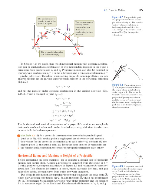
In Section 4.2, we stated that two-dimensional motion with constant accelera-
tion can be analyzed as a combination of two independent motions in the x and y
of a projectile that leaves the origin with a velocity Sv i. The velocity vector Sv changes with time in
both magnitude and direction.
AVL标准

2
1
0 0 0,5 1 1,5 2 2,5 3 3,5 4 4,5 5 5,5 6 Oil Supply Pressure [bar] Report DAV0003 Attachment-03 / Page 14
Main Results of PCJ Flow Tests
Item PCJ opening pressure [bar] PCJ closing pressure [bar] Result observed 2.2 – 2.3 2.0 – 2.3 AVL Guideline 1.2 – 1.6 ---
2 Closing 1 Opening
Oil pressure range at rated sped / rated power TWO = 85 - 110 ° C
0 0 0,5 1 1,5 2 2,5 3 3,5 4 4,5 5 5,5 6 Oil Supply Pressure [bar]
Report DAV0003 Attachment-03 / Page 12
Oil supply pressure = 2.4 bar Oil supply pressure = 2.5 bar
Oil supply pressure = 3.0 bar
Oil supply pressure = 3.5 bar源自Report DAV0003
Attachment-03 / Page 6
Report DAV0003
Attachment-03 / Page 15
Conclusion and Recommendation For the D4 EU4 Stage2 4-cylinder engine the measured oil flow rates are slightly above the AVL guideline considering a rated power of 120 kW For the D6 EU4 Stage2 6-cylinder engine the measured oil flow rates are in the upper range of the AVL guideline considering a rated power of 202 kW The visual spray quality is satisfying up to the relevant oil supply pressure of 4 bar The layout of the piston cooling jets has to be checked by piston temperature measurements at rated power conditions and max. continuos coolant temperature level on both engine types D4 and D6
中英文文献翻译—变速器油温的控制
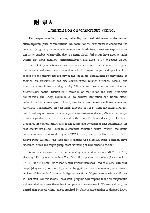
附录ATransmission oil temperature controlFor people who buy the car, reliability and fuel efficiency is the second oftwoimportant price considerations. No doubt, for the new owner is concerned, the most terrifying thing on the way to remove car. In addition, owner and expect the car can try to durable. Meanwhile, due to current global fuel prices have risen to make owners pay more attention。
thefuelefficiency, and hope to try to reduce carbon emissions. Auto power transmission system includes an internal combustion engine, transmission and more than a gear than wheels. Engine torque and speed will be needed for the railway traction power and car in the transmission of conversion. In addition, the transmission can also control wheel rotation direction. Manual and automatic transmission speed generally fall into two. Automatic transmission can automatically control friction unit, selection of gear ratios and shift. Automatic transmission will adopt hydraulic oil to achieve lubrication and frozen effect, hydraulic oil is a very special liquid, can be in any severe conditions operation. Automatic transmission oil (the main function of ATF) from the motivation for: transferred engine torque converter power transmission device; Absorb the torque converter produces thermal and moved to the front of a frozen device; car As clutch friction of the coolest refrigerants, it can absorb and by clutch or take out meshing the heat energy produced; Through a complex hydraulic control system, the liquid pressure transmission to the system USES valve, servo machines, pump, clutch always pump, hydraulic pipe and pipe to control; As a planetary gears, bearings, servo machines, clutch and target group-exact marketing of lubricant and coolant.Automatic transmission oil in operating temperature (about 90 °C / °F) viscosity 195 is general very low. But if the oil temperature is too low (for example is 0 ° C / 30 °F below), its viscosity will greatly increased, lead to a very high drag torque (dragtorque). As a result, gear meshing, it can cause is commonly synchronous devices of this couldn't cope with high torque force. If gear can't mesh or shift, car will not start. For this reason, "cold start" program will respond to the oil temperature and activated, to ensure that at least one gear can succeed mesh. Warm car driving car started after process when, unless required by obvious acceleration or dragged heavyobjects (such as trailer), otherwise the hydraulic oil temperature will only slowly rising, but it also means drag torque will slowly rising. If the car is chronically high drag torque environment, synchronous devices will overload and damaged. In gearbox to add some loss, will shift some moved to higher speed valve and improve the quality of the gearbox lubricant, these all can accelerate the process of car warm up. Thus, engine, gearbox and catalyst can be quickly reach best operation temperature. The faster transmission is the optimum operating temperature, can be used to save fuel consumption and faster start the gear shift program. Gear shifting part through hydraulic or electronic is starting valve to control, these shifting unit start-up will significantly by the influence of the temperature of automatic transmission oil, reason is with the temperature and the viscosity will rise significantly, so the temperature can influence the degree of pressure and time characteristics. Once the automatic transmission oil gets hot, its temperature variation of amplitude will increase, so the shift when the set standard oil, must consider the problems about the oil temperature. Under high temperature operation, no doubt, automatic transmission oil very vulnerable to the influence of the temperature of cryogenic, but compared to the reaction of the reaction temperature, the much more. The process of automatic transmission will produce a lot of friction, and these will generate a lot of friction heat. Liquid will constantly stir in torque converter and pump in the mouth and current meters of hydraulic circuits. Whenever variable speed shift, clutch components will produce more than box of oil can take the heat. The transmission, the greater the load of the heat generated by then, box of oil will become more heat. General traditional transmission oil temperature can allow maximum temperature for 80 to 100 °C or 175 ° F, and to 212 special transmission oil temperature can be as high as 110 ℃to 130 °F or 230 to 265. However, nowadays advanced automobile transmission oil temperature could be as high as 120 to 150 ℃or 250 to 300 °F, and for heavy trucks for example is 18 rounds of freight trains, if it in hot weather, the oil temperature under driving even to 170 °C 160 °F or 320 to 340. Such a high oil temperature can cause box of oil and variable speed component damage. Transmission oil working life, in the high temperature environment, the working life of the transmission oil can be reduced. Once the temperature above normal operation level (90 °C / 195 °F above), lubricants oxidation speed will increase, so the effective life be shortened. Based on the law 娒designated, when the temperatureabove normal operation temperature 。
D_B传热关系式
M.HEAT MASS TRANSFERVol.12, pp.3-22, 1985Printed in the United StatesHeat Transfer In Automobile Radiators Of The Tubular Type(管状换热器/暖气片)F. W. Dittus and L. M. K. BoelterIntroductionHeat to be dissipated from water-cooled internal combustion engines is usually transferred to the atmosphere by means of devices commonly called radiators. The medium conveying heat to the radiator is generally water, the medium conveying heat away is air.In this article it is intended to discuss the fundamentals involve in the transfer of heat from water to the atmosphere in the simplest type of tubular radiator. No attempt will be made to discuss the effect of the rate of heat transfer when using fins, honeycomb section, or any type other than the plain tube.The unit of measure of heat transfer in heat exchange equipment is the “Overall Transfer Factor”, which is the heat transferred per unit area of heat transmitting surface per unit time per unit of temperature difference between the hot and cold fluids.Film Transfer Factor On The Liquid Side Of A RadiatorTypes of fluid flour through tubesOn the liquid side of a radiator heat is carried from the warm water to the colder tube wall by two methods:(1)Convection(2)ConductionIn the region of turbulent flow, most of the heat is transferred from the liquid to the tube wall by forced convection. Because of the low thermal conductivity of fluids, very little heat is transferred from the center of the stream to the tube wall by conduction. In forced circulation systems the fluid flow through the radiator is turbulent unless the tubes are of very small diameter.In the viscous flow region practically all of the heat is transferred from the interior of the stream to the tube wall by conduction.The rate of heat flow from the water to the air is retarded by(a)Film resistance on the water side of the tube surface,(b)Thermal resistance of tube,(c)Film resistance on the air side of the tube.If we denote the three resistances mentioned above by R w, R t, and R a, respectively, we may write the following equation:(1)o w t a R R R R =++where R o =overall or total heat flow resistance.Ordinarily, however, the term employed is not thermal resistance but thermal conductance, which is the reciprocal of resistance. Denoting thermal conductance by U we may then write:1111(2)o w t aU U U U =++ whereU o =overall transfer factor (BTU/sq.ft./℉./hr.).U w =film transfer factor on water side (BTU/sq.ft./℉./hr.).U a =film transfer factor on air side (BTU/sq.ft./℉./hr.).U t =thermal conductance of separating wall (BTU/sq.ft./℉./hr.).The value of U t can be readily calculated by the use of the following equation:(3)t kU t =wheret=thickness of separating wall (ft.).k=thermal conductivity of separating wall material (BTU/sq.ft./℉./hr.).Equation (2) holds when heat is transferred through a body with parallel heat-transmitting surfaces. In the case of heat flow through curved surfaces, for example, tube walls, a correction should be made for the face that the outer surface per unit length of tube is greater than the inner surface for the same length of tube. Equation (2) then becomes:1111(4)?o m a a t t w w U A U A U A U A =++ or, referred to the mean diameter of the tube, equation (4) becomes:1111(5)'o w t a U U R U U R =++whereA m =Mean area of heat transfer section based on mean tube diameter (sq.ft).A a =Area of heat transfer section on air side (sq.ft).A w =Area of heat transfer section on water side (sq.ft).R=Ratio of outer tube surface (air) to surface of tube at mean diameter per unit length of tube.R ’=Ratio of inner tube surface (water) to surface of tube at mean diameter per unit length of tube.R=2D/(D+d).R ’=2d/(D+d).D=Outside diameter of tube (inches).d=Inside diameter of tube (inches).The value of U t for a curved separating wall is:4(6)()ln /t kU D d D d =+Substituting equation (6) for the term U t and also substituting in equation (5) the equivalent values of R and R ’, the latter becomes:11ln /1()()(7)?22o o t D d D d U U D k U D+=++The type of fluid flow existing within a tube may be determined by calculating “Reynolds criterion ”, which is defined as follows:(8)/0.624r vd Vd C u s z == whereC r =Reynolds criterionC r ’=Reynolds critical number (see following paragraph)v=mean linear velocity of fluid (ft./sec.)V=mean mass velocity (lbs./sq.ft./sec.)d=inside diameter of tube (inches)u=absolute viscosity of fluid at mean stream temperature (poises) z=absolute viscosity of fluid at mean stream temperature (centipoises)s=density of fluid (numerically equal to the specific gravity of fluid referred to water at 60℉.) (gram./cc.)If, upon substitution of the proper values in the above equation, the numerical result (Cr) is greater than 40, the flow is turbulent. If, on the other hand, the result is less than 25, the flow is non-turbulent or viscous. In the event that a ratio (Cr ’) having a value between the just mentioned numbers is obtained, the flow may be either turbulent or viscous depending to a great extent upon the entrance and exit conditions of the installation in question and roughness of the tube surface.Film transfer factors for turbulent flow —Most of the experimental work done on heat transfer covers the turbulent region for fluid flow inside of tubes. McAdams and Frost (1922) correlated all the published data and proposed the following equation for heat transfer existing at turbulent flow:0.7961()(9)/Ud vd B k u s = which is a simplified form of the following equation proposed by Nusselt (1910): 12()()(10)/Ud vd cu f f k u s k =WhereB1=constant c=specific heat of fluid (BTU/lb./℉) k=thermal conductivity of fluid (BTU/sq.ft./hr./℉./ft.),and all other terms as mentioned above.McAdams and Frost eliminated the third term of equation (10) because the correlated datafell along the same straight line when plotted on logarithmic paper according to equation (9). Most of the data plotted were results of heat transfer tests conducted with water flowing through tubes.Equation (9) was later modified by McAdams and Frost (1924) to include a correction for the increased heat transfer rate due to turbulence at the entrance of the tube. This modified equation is as follows:2(1)()(11)'/Ud N vd B f k r u s=+ whereB2=constantN=empirical numberr=ratio of tube length to diameter=l /du ’=viscosity of fluid at film temperature (poises) Upon considering the results a number of experiments the equation proposed by the last mentioned authors was:0.80250(1)()(12)?'/Ud vd B k r u s =+As mentioned above, in most of the experiments performed the fluid used was water and the heat was generally flowing from the tube to the liquid, i.e., heating the liquid.Morris and Whitman (1928) conducted a series of experiments in which oils having a wide range of viscosities were used. In addition to this they studied the heat transfer rates for cooling as well as heating of the liquid flowing through the tube. The result of the investigation showed that film transfer factors may be expressed by the following equation:0.37()()(13)?Ud Vd cz f k z k =which is of the same form as the Nusselt equation previously mentioned, except that mass velocity (lbs./sq.ft./sec.) is used instead of linear velocity and absolute viscosity expressed in centi-poises instead of poises. The two just mentioned variables are denoted by “V ” and “z ” respectively. Figure 1 shows the experimental data of these investigators plotted according to equation (13). It will be noted that there are two separate groups of points, one for heating liquids and another for cooling liquids. As pointed out by Morris and Whitman, the film transfer factor for cooling a liquid is about 75 per cent of that for heating a liquid when the comparison is made at the same flow conditions.This variation is no doubt due to the fact that the physical properties of the fluid particles conveying and conducing heat are different for the two conditions, even though the mean fluid temperatures are the same. Perhaps a better procedure would be to plot the film transfer factoes as a function of the various thermal properties of the fluid at the film temperature instead of the mean stream temperature.The curves obtained when using the physical properties of the fluid at the tube temperature instead of at the mean stream temperature are in no better agreement than those shown by Morris and Whitman, nor is there a better agreement when the physical properties are taken at a mean temperature between the tube wall and mean stream temperatures. In every case a separate curve was obtained for heating and cooling, in some cases the cooling curve lying above and in some cases lying below the heating curve, depending entirely upon the temperature used to determine the physical properties of the liquid.In order to obtain a common curve for heating and cooling, it is suggested to use two different exponents in the term (cz/k)n for each process. Figure 2 shows the plotted results calculated from Morris and Whitman ’s published data, using n equals 0.4 and 0.3 respectively for heating and cooling a liquid flowing to a tube. Unfortunately, no other data are available to test the use of two different exponents for heating and cooling.The fluids used by Morris and Whitman in their experiments were water and oils covering a considerable range of viscosities. Neither these authors nor McAdams and Frost showed any experimental values for gases flowing through tubes.In order to determine whether or not the Morris and Whitman curve also applies to gases, the published results of a number of investigators using gases in their heat transfer experiments were analyzed and plotted according to the following equations:()()(14)z nUd Vd cz f k k wheren=0.3 for coolingn=0.4 for heatingall other variables as previously defined.The curves thus obtained for gases are shown in figure 3 together with others published by McAdams and Frost for liquids. The curves shown for gas flow cover a range of tube diameters from 1/2 inch to about 6 inches and a temperature range from 60℉ to 1400℉. The mass velocities varied from 0.2 to 6.6 lbs. per sq. ft. per second. The pressure within the pipe varied from 1.5 to 190 pounds per sq. inch absolute. Considering this wide variation in operating conditions, the agreement of the curves is remarkable, although it is somewhat difficult to draw a mean curve.The mean curve shown on figure 3 may be expressed by the following equation:19.5()()(15)m nUd dV cz k z k =where n is the 0.3 and 0.4 for cooling and heating, respectively, as mentioned above.The entrance correction factor (1+50/r) proposed by McAdams and Frost was omitted by Morris and Whitman in the equation proposed by the latter . The reason for the omission is that not sufficient data are available definitely to determine the end correction factor. For the same reason the factor is also omitted from equation (15).Film transfer factor for viscous or non-turbulent flow —Very little data have been published on heat transfer for viscous flow. McAdams (1925) published a curve having a slope of about 1/10 when the variable (l ’d/k)/(1+50/r) is plotted against (Vd/z) or, in other words,1/1150()(1)(16)?o Ud Vd B k z r=+No experimental data were shown to support this equation.Some experiments were conducted by Dittus at the University of California (1929) on the heat transfer from tubes to liquids in viscous motion. It was found upon plotting the experimental results according to the equation Ud/k=f(Vd/z) that the latter equation did not hold, but separate curves were obtained, each of which had a slope of roughly 1/12, for each diameter tube tested. It was apparent that some additional variables should be included in the above equation in order to obtain a satisfactory curve. When the experimental data were plottedaccording to Nusselt ’s equation (10), the results again did not fall along the same curve. Upon including the additional variables, specific heat and temperature difference, the following equation was derived by the application of the principle of dimensional homogeneity:3U [(),(),()](17)/d rd drsc k f k u s k dv s ∆=where △=logarithmic mean temperature difference between tube and liquid, and all other terms are the same as mentioned before.By combining the variables in equation (17) in a particular manner, it was possible to derive a new group of variables, which caused all experimental points to fall along the same curve when plotted accordingly.The final equation proposed is as follows:1/32/31/1220()()(18)/k vd U s c d u s ∆= Further information on heat transfer in the viscous or non-turbulent flow region is available in an article published by Thomas and Wadlow (1929) on the heat transfer performance of tubular radiators for automobiles. These investigators determined the overall transfer from water to air by maintaining a constant water velocity and varying the air velocity in one set of experiments. These tests covered both the turbulent and the non-turbulent or viscous flow on the water side of the turbulent and the non-turbulent or viscous flow on the water side of the radiator tubes. Because of the method employed of varying only one of either the air or water velocity, it is possible to calculate the film transfer factors from the overall transfer factors. The results are shown in figure 4.It will be noted upon reviewing figure 4 that results calculated from Thomas and Wadlow ’s data do not agree with the tests of Dittus. The reason for this may be that in the latter tests every effort was made to eliminate turbulence due to entrance and exit, disturbances, while in the former tests no such precaution was observed. For this reason, turbulence existed at the entrance to the radiator tubes, which may have resulted in a higher overall transfer factor.It will be remembered that McAdams and Frost suggested an end correction factor for the case of turbulent flow.Upon applying the same correction factors (1+50/r) to the results calculated from Thomas ’ and Wadlow ’s data and plotting the values thus corrected, it was found that the plotted points coincided remarkably well with those reported by Dittus (1929), as is shown in figure 5. The equation now proposed for heat transfer existing at viscous flow is as follows:1/32/31/125020()()(1)(19)/k vd U s c d u s r ∆=+ As mentioned above, in the tests conducted by Dittus provisions were made to eliminate all disturbance due to entrance conditions. For that particular case the term r then becomes infinite and equation (19) will be the same as equation (18).It is true that the introduction of the end correction term is based on rather meager data, but until more data are available, it is advisable to employ the McAdams and Frost end correction factor as shown in equation (19).Film transfer Factor With Flow Transverse to TubesSingle row of tubes —Much work has been done on heat transfer from cylinders to fluids and vice versa with flow at right angles to the cylinder. Some experiments have been conducted with heated wires moving at a fixed velocity through liquids or air in order to obtain a relation of heat transmission and relative velocity and thus calibrate the device for velocity measurements. Some work has also been done with air flow transverse to tubes. The most recent data of the latter type of tests are those published by Reiher (1925) in which hot air was cooled by flowing transverse to cold tubes. Reiher proposed the following equation:()(20)/m m m mv D UD f k u s =which may also be expressed as follows: ()(21)m m mv D UD f k z = wherev m =average velocity between two adjacent tubes (ft./sec.)V m =average mass velocity between two adjacent tubes (lbs./sq.ft./sec.)D=absolute viscosity of fluid at mean of tube and fluid temperature (poises)u m =absolute viscosity of fluid at mean of tube and fluid temperature (poises)z m=absolute viscosity of fluid at mean of tube and fluid temperature (poises)k m =thermal conductivity of fluid at mean of fluid and tube temperatures (BTU/sq.ft./hr./℉/ft.)c m =specific heat of fluid at mean of fluid and tube temperature (BTU/lb./℉)and all other terms are as mentioned before.The term Vm may be calculated as follows:(22)4m o bV V d b π=-also max(23)o b D V V b -= whereVo=mass velocity of gas just before entering tube bundle (lbs./sq.ft./sec.)Vmax=maximum mass velocity of gas between two adjacent tubes (lbs./sq.ft./sec.)b=center to center spacing of tubes (inches)D=outside diameter of tubes (inches) Using the term Vm instead of either Vo or Vmax eliminates the use of another group of variables involving the ratio of tube spacing to tube diameter. Reiher found that upon plotted in that manner in figure 6. It will be noted that points obtained with air flowing at right angles to the cylinder fall along the same curve, while the points obtained from experiments using oil and water instead of air formed separate curves depending upon the liquid used.Expressing each curve according to the following equation:()(24)nm o m m V D UD B k z =It was found that the constant B 0 could be plotted as a function of the term (c m z m /k m ) and varied as the one-third power of the last-mentioned group of variables.Because of this fact all data were replotted as shown in figure 7 according to the following equation:1/3()()(25)n m m m m m m v D c z UD f k z k =Upon reviewing figure 7 it will be noted that all points, regardless of whether tests were conducted with water, oil, or air, fall along the same curve. It will furthermore be noted that for the region where V m D/z m is less than 0.25 the line has a slope of 0.4 while for the region above that the line has a slope of about 0.56. Apparently there is a change of film conditions at the intersection of the two curves. The equations for heat transfer with fluid flow at right angles to cylinders may then be written as follows:(a) for 0.25m mV D z < 0.41/383()()(26)m m m m m mV D c z UD k z k = (b) for 0.25m mV D z >0.541/3105()()(27)m m m m m m V D c z UD k z k =Several rows of tubes —A series of tests for the determination of heat transfer when several rows of tubes are involved were made by Reiher. In all these experiments the heat transfer took place from tubes to air; no data are available from experiments in which liquids were used. Furthermore, all of Rerher ’s results are for the region where V m D/z m is greater than 0.25 so that no data are available ta all for several rows of tubes in the region where the just mentioned criterion is less than 0.25. Until experiments prove otherwise, it may be assumed that Reiher ’s equation applying to airflow only may be modified to include liquid flow by introducing the term (c m z m /k m )1/3 as wasdone in the case of the equations for single tubes. The modified equations applying to several rows of tubes for the region where V m D/z m is greater than 0.25 are as follows:(1) staggered rows of tubes: 2 rows,0.691/3max 53()()(28)?m m m m mV D c z UD k z k = 3 rows, 0.691/3max 60()()(29)?m m m m mV D c z UD k z k = 4 rows, 0.691/3max 65()()(30)?m m m m mV D c z UD k z k = 5 rows, 0.691/3max 69()()(31)?m m m m m V D c z UD k z k =(2) rows of tubes directly behind each other: 2 rows,0.6541/3max 55()()(32)?m m m m mV D c z UD k z k = 3 rows, 0.6541/3max 57()()(33)?m m m m mV D c z UD k z k = 4 rows, 0.6541/3max 58()()(34)?m m m m mV D c z UD k z k = 5 rows, 0.6541/3max 59()()(35)?m m m m m V D c z UD k z k =It should be noted that in the two last mentioned groups of equations the term V max instead of V mean is used. Just why this was done is not explained in Reiher ’s paper; unless he assumes that in heat exchange equipment, when several rows of tubes are used, the bulk of the heat transfer takes place at the point of maximum velocity. Rerher also states that the above equations are valid only when the tubes are fairly clos together.Discussion and conclusionsAnalysis of published data on heat transfer in tubular radiators indicates that a large part of the total resistance to heat flow is due to the relatively low film transfer factors on the air side of the tubes. For this reason, any attempt to increase the overall transfer factor on the air side of the tube. Some improvements may also be made by decreasing the film resistance on the liquid side of the tubes, although the total gain will be slight unless the air film transfer factor is increased materially at the same time. The film transfer factor on the liquid side of a tubular radiator may be calculated readily with the aid of the equations (15) and (19) according as the flow is turbulent or non-turbulent respectively.The critical point at which the flow within a tube changes from non-turbulent to turbulent may be determined by application of Reynolds criterion listed as equation (8).It appears that there is also a critical region for flow transverse to tubes at which the flow changes from non-turbulent or viscous to turbulent; this is clearly shown in figure 7. The change of flow from non-turbulent to turbulent appears to take place at the point where V m D/z m is equal to 0.25.For the non-turbulent or viscous region of flow transverse to tubes the film transfer factor for single rows of tubes is expressed by equation (26) while for the turbulent region equation (27) applies.。
自由活塞斯特林发动机Re-1000的模拟研究
自由活塞斯特林发动机Re-1000的模拟研究陈曦,崔浩(上海理工大学能源与动力工程学院,上海200093)摘要:为了掌握自由活塞斯特林发动机的设计方法,采用Sage 软件建立了自由活塞斯特林发动机Re-1000的一维模型。
模拟结果和实验结果比较显示,输出功率、热效率的模拟值和实验值呈相同的变化趋势。
输出功率模拟值与实验值误差约为15%,热效率模拟值比实验值大4%。
证明了Sage 软件模拟自由活塞斯特林发动机具有较好的准确性,对优化自由活塞斯特林发动机性能有一定意义。
关键词:自由活塞斯特林发动机;Re-1000;数值模拟;SAGE 中图分类号:TK124;TB651+.5文献标志码:A文章编号:1006-7086(2018)05-0304-05DOI :10.3969/j.issn.1006-7086.2018.05.003Simulation Study on Re-1000Free-piston Stirling EngineCHEN Xi ,CUI Hao(School of Power and Energy Engineering ,University of Shanghai for Science and Technology ,Shanghai200093,China )Abstract :In order to find out design methods of the free piston Stirling engine ,Sage software is used to establish a one-dimensional model of the free piston Stirling engine (Re-1000).The simulation results are compared with the experi-mental results.The simulation results showed the same changing trend with the experimental results in the values of the output power and thermal efficiency.The error of output power between the simulation value and the experimental value is about 15%.The simulation value of thermal efficiency is 4%larger than the experimental value.It is proved that the Sage software can simulate the free-piston Stirling engine with good accuracy.And this effort has certain significance on opti-mizing the performance of the free-piston Stirling engine.Key words :free-piston Stirling engine ;Re-1000;numerical simulation ;SAGE0引言1816年,苏格兰牧师Robert Stirling 发明了斯特林发动机(又称热气机),是一种外燃、闭式循环、往复活塞式的能量转换装置[1]。
residual stresses in quenched aluminum blocks and their reduction through cold working processes
Journal of Materials Processing Technology174(2006)342–354Prediction of residual stresses in quenched aluminum blocks andtheir reduction through cold working processesMuammer Koc¸a,∗,John Culp b,Taylan Altan ca Department of Mechanical Engineering,University of Michigan,Ann Arbor,MI48109,USAb Weber Metals,Paramount,CA,USAc ERC for Net Shape Manufacturing,Ohio State University,Columbus,OH,USAReceived26November2004;received in revised form31January2006;accepted1February2006AbstractResidual stresses developed after quenching of aluminum alloys cause distortion during subsequent machining.As a result,machined parts may be out of tolerance and have to be cold worked or re-machined.Experimental measurement of residual stresses is lengthy,tedious and very expensive even with the latest developments in neutron X-ray diffraction techniques,for instance.Therefore,in this study,numerical techniques are used to predict residual stresses after quenching of Al7050forged block,and the predictions were compared with experimental measurements. The results indicated that the predicted values are in very good agreement with the experimental measurements with around10–15%deviation in the worst case.Two different methods of cold working(compression and stretching)are used to reduce the residual stresses.The comparison of results showed that both compression and stretching processes reduced the residual stresses more than90%.However,single-strike compression of aluminum blocks is found to be more efficient and cost-effective for reducing the residual stresses to very low levels.The effects of elastic die were also investigated.Die deflection was found to affect the residual stress reduction capability negatively by decreasing the magnitude of stress reduction from90%to about70%.©2006Elsevier B.V.All rights reserved.Keywords:Residual stress;Quenching;Stress relief;FEA predictions;Aluminum1.IntroductionResidual stresses are the system of stresses that exist in a body when it is free from external forces.They are the consequences of heat treatment[1–5],deformation processes[6,7],machining [8],welding/joining[9]or combinations of above that transform the shape and/or change the properties of materials.Residual stresses develop when a body undergoes inhomogeneous plastic deformation or is exposed to a non-uniform temperature distri-bution such as in the case of casting,warm forming,welding and quenching processes.In general,the sign of residual stress will be opposite to the sign of the plastic strain which produced the residual stress,e.g.in the case of a rolled sheet,the residual-stress pattern consists of a high compressive stress at the surface which was elongated in the longitudinal direction by rolling. After removing the external force,there is compressive stress at the surface and tensile stress at the center of the sheet.The ∗Corresponding author.Tel.:+17347637119;fax:+16465147590.E-mail address:mkoc@(M.Koc¸).importance and relevance for the measurement,prediction and control of residual stresses are based on their effect on manufac-tured products.Residual stresses may induce premature failure through cracking,reduce fatigue strength,induce stress corro-sion or hydrogen cracking,and cause distortion and dimensional variation.On the other hand,compressive residual stresses may improve fatigue life,stress corrosion,or hydrogen embrittle-ment of a component[10–13].Therefore,the investigation and understanding of residual stress measurement,prediction and reduction/induction is important to improve the quality and reli-ability of many manufactured parts.Residual stresses cannot be measured directly[9,11,14]. What is measured is the elastic strain caused by the residual macro and micro stresses.Some of the measurement methods used in the practice are:(a)ultrasonic method is based on the fact that when a crystalline material is placed under stress,the velocity of the ultrasound changes,and with suitable instrumen-tation and techniques,the change in velocity can be measured;(b)mechanical methods have been used longer than any of the other methods.There are different approaches,and most of them consist of the removal of stressed material and the measure-0924-0136/$–see front matter©2006Elsevier B.V.All rights reserved. doi:10.1016/j.jmatprotec.2006.02.007M.Ko¸c et al./Journal of Materials Processing Technology174(2006)342–354343ment of the resultant strain change.The most popular technique currently in practical use is the hole drilling method[14,15]. Other mechanical methods are the removal of layer method (Treuting-Read Method)and the deflection method[2,14];(c) X-ray diffraction method:When a metal or ceramic polycrys-talline material is placed under stress,the elastic strains in the material occur in the crystal lattice of each single grain.The stress applied externally or that is residual within the material, as long as it is under itsflow stress,is taken up by interatomic strain.The X-ray diffraction techniques are able to measure the interatomic spacings,which are characteristic for the macros-train undergone by the specimen[11,14,16].Since neutrons have a higher penetration than X-rays,they can be used as well [7,14,16,17].Relief of residual stresses can be achieved through the mechanical methods of compression and stretching as well as heat treatment methods such as tempering[3,18–21]in addi-tion non-traditional approaches such as pulsed magnetic treat-ment[22].Stretching is known to be very effective in reducing the residual stresses based on both production and experimen-tal results[10,20].However,since stretching non-rectangular and non-symmetric parts is not practical because of handling problems and asymmetric loading,compression processes are usually preferred.Availability of equipment,existing capabil-ities and cost factors determine the method used for relieving residual pression has been applied only to parts with simple shapes and parallel surfaces,and in addition,the thickness of the workpiece had to be less than the maximum allowable heat-treat section thickness[23].Prediction of residual stresses with analytical or numeri-cal methods has been studied extensively since experimental measurement of residual stresses is very lengthy,tedious and expensive.Due to its versatility,accuracy and efficiency,finite element analysis(FEA)technique is found to be a viable and cost-effective alternative[7,13,24,25].In thefirst section of this paper,FEA is demonstrated to predict residual stresses in quenched aluminum blocks with reasonable accuracy,com-pared with experimental measurements performed using neutron diffraction method.In the second section,analysis and improve-ment of stress relief processes were accomplished using FEA eliminating the costly and lengthy residual stress relief trials conducted on the plantfloor.Finally,the effect of die/tooling elasticity on the relief of residual stresses during compression is presented.2.FE analysis of quenchingQuenching is a heat treatment method where a hot metal part is cooled down rapidly with the help of a quenchant such as water,oil,other liquids,or combinations of them[3–5,26]. The use of FEM for the analysis of the quenching process for aluminum parts has been performed earlier[7,13,24,27].The predicted results showed good agreement with the experimental values of residual stresses with a range of4ksi(25N/mm2) as measured by a layer removal method[24].The quenching conditions have a major influence on the residual stresses,e.g. aluminum quenching in“cold”water(68◦F(20◦C))occurs in Table1Quenching process conditions,and Elastic Modulus(E)and Poisson ratio(ν) for Al7075[24]Parameters Symbol Value Block temperature before quenching T0477◦C Quenchant temperature T∞66◦C Block temperature after quenching T166◦C Quenching time t500sE(N/mm2)T(◦C)ν7245000.29 696901000.29 648602000.29 586503000.29 538204000.29For values beyond400◦C,extrapolation was performed.a50%higher range of residual stress than quenching in“hot”water(176◦F(80◦C))[24,26,28].2.1.Quenching process conditionsIn this study,FE analyses were performed for both quenching and subsequent stretching and compression processes.For the quenching process,FEA conditions were taken from the experi-ments as documented in a report by Boeing and its suppliers[29]. The authors of this paper were not involved in the experiments and measurements,but were provided with the report of which some section cannot be disclosed.In the quenching process, aluminum blocks of7050alloys with a uniform temperature of 477◦C were immersed in water at a temperature of66◦C until the aluminum block was cooled down to a uniform tempera-ture.Therefore,a coupled temperature–displacement analysis was required to(a)determine the temperature variations as a function of time during quenching(heat transfer analysis)and (b)calculate residual stresses due to temperature changes(stress analysis).Two different Al7050blocks were used in this study (Fig.1).In thefirst case,a7050aluminum block of 340mm×127mm×124mm(Block A)was used for validation of FEA through comparison with experimental measurements conducted using neutron diffraction method by the sponsoring company.In the second case,residual stress formation and relief on aluminum blocks of1270mm×406mm×127mm(Block C)were analyzed as this type of blocks were commonly used as the raw material for forging and machining to manufacture aircraft structures.A7050is a typical tempered aluminum alloy used in the aircraft industry.In our analyses,since material and physical data was not available for Al7050tempered aluminum-forged blocks,data for Al7075was used instead.This was a reasonable approximation because both alloys have similar compositions[30,31].Table1presents the quenching process conditions.Tables2–5describe the material properties used in this study.Elastic-perfectly plastic FE analysis of the quench-ing process was performed using ABAQUS/Standard.It was assumed that there were no stresses in the block at the beginning since the block was heated and held at477◦C,which is above344M.Ko¸c et al./Journal of Materials Processing Technology 174(2006)342–354Fig.1.(a)Block A (340mm ×127mm ×124mm),(b)Block C (1270mm ×406mm ×127mm):dimensions,FE model and the mid-plane used for measurements.the recrystallization temperature of 7050aluminum alloys [31].Since the geometry and the boundary conditions were all sym-metrical,a simplification of the FE model was possible by using 1/8of the blocks to reduce the CPU time for the simulations.The FE model used for Blocks A and C in the present study are illustrated in Fig.1.This figure also shows the planes where residual stresses in the X ,Y ,and Z directions were measured and reported.2.2.Results of the quenching FEA for Block AExperimental measurement data using X-ray neutron diffrac-tion method was only available for Block A.Therefore,aTable 2Stress–strain values for Al 7075at room temperature [35]and yield strength at different temperatures [1]Stress (N/mm 2)at 25◦C Strain 2210.02860.052890.12900.153040.23170.253570.53680.6Yield strength (N/mm 2)T (◦C)22166212250150300873506040026477quenching analysis is performed for this case to verify the accu-racy and effectiveness of the coupled temperature–displacement FE analysis by comparing the predictions with the results of the experiments.The stress distributions obtained from the experi-mental measurements are not exactly symmetric.This may be because (a)the block was not entirely stress-free before it was heated;(b)there might have been deviations during measure-ments;and (c)a non-uniform and non-symmetric quenching process might be caused by slow immersion into the quenchant.Overall,all of the curves for Analysis #2and the experimen-tal results are in good agreement with an approximate deviation of 14%.The maximum difference between the experimental and Analysis #2results is in the range of ±70N/mm 2.An additional FE analysis step of air cooling after quenching from 66◦C to room temperature (20◦C)did not affect the results more than ±2.5%.Therefore,this step was neglected in the following anal-Table 3Density and thermal expansion of Al 7075for different temperatures [1]T (◦C)Density (g/cm 3)2.79602.7681002.7682002.7403002.7134002.6855002.657600Thermal expansion (10−6K −1)21.82023.610024.520025.4300M.Ko¸c et al./Journal of Materials Processing Technology174(2006)342–354345parison of x-,y-and z-component residual stresses on Block A along x-locus at the middle plane for experimental,and Analysis#2results.yses.Figs.2and3illustrate the x-,y-and z-component residual stresses after quenching along the x-and y-loci at the middle plane for Analyses1and2,and the experiments.In all three cases,there is a symmetric stress distribution with tensile resid-ual stress at the center and compressive residual stress at the surface.The values of the x-component stresses along the x-locus are lower when compared to the other components.The results of Analysis#2match the experimental results very well except for the z-component stresses where the experimental results are approximately5ksi(35N/mm2)higher then the FEMresults. parison of x-,y-and z-component residual stresses on Block A along y-locus at the middle plane for experimental and Analysis#2results.346M.Ko¸c et al./Journal of Materials Processing Technology 174(2006)342–354Fig.4.Distribution of x -,y -and z -component residual stresses (psi)on Block A after Analysis #2along 1/4of the middle plane.Overall,all of the curves,Analysis #1,Analysis #2and theexperimental results are in good agreement.Fig.4shows the dis-tribution of the x -,y -and z -component residual stress of Block 1after Analysis #2at the middle plane.Table 4Thermal conductivity and specific heat of Al 7075for different temperatures [1]convection coefficient (h)between aluminum and water [36]T (◦C)Thermal conductivity,k (kW/m K)0.1100.121000.142000.153000.164000.17500Specific heat,h c (J/kg K)8372089610096320011304001193477Convection coef.,h (Al and water),×106(kW/m 2K)200.1504.01009.015013.520017.525016.030013.035011.04009.04507.05005.85502.3.Results of the quenching FEA for Block CA similar quenching analysis (Analysis #3)was performed using the Block C.It had the same boundary conditions and the same simulation steps as in Analysis #2.The geometry of Block C as well as the middle plane and the FEM model used are shown in Fig.1b.Fig.5illustrates the predicted x ,y and z residual stress components at the x -and y -loci at the middle plane.Fig.6presents the distribution of x ,y ,and z stress components in a quarter of the model at the mid-plane.As it is observed from these figures,the maximum tensile stresses are at the center for the x and z residual stresses.The compressive stresses are at the surfaces.Since the cross section of Block C is rectangu-lar rather than square,the y -component residual stress is lower than the x -and z -component.At the edge,the y -componentTable 5Conditions of compression FE analyses Analysis #ProcessFriction factor billet/die ()Lubrication condition 5Compression—1%0.4Dry [32]6Compression—2%0.47Compression—4%0.48Compression—1%0.05Lubricated(Teflon,PTFE as in [33])9Compression—2%0.0510Compression—4%0.05Compression ratios 1–4%(0.127–0.508mm)Compression speed 20mm/s Block temperature66◦CM.Ko¸c et al./Journal of Materials Processing Technology174(2006)342–354347Fig.5.Predicted residual stresses for Block C along x-and y-locus at the middle plane.residual stress is compressive(−242N/mm2)while it becomes tensile(55N/mm2)at a distance33mm from the edge.At this region,where the distance to the edge is the same as the distance to the top and/or the bottom surfaces(1/2times thick-ness=2.5in≈0.15fraction),the y-stress reaches its highest value(55N/mm2),i.e.edge effect.Towards the middle region of Block C,the y-component starts going down to zero as the edge effect loses its influence.In this case the major influence of the geometry on the developing residual stresses is shown very clearly.Since the z-dimension of the plate is the largest, the z-component residual stress always has the highest values up to221N/mm2(i.e.the larger the dimension,the higher the temperature gradient,in turn,the higher the residual stresses). Along the y-locus the stress distribution is easy to explain.The z-component again reaches the highest tensile value of221N/mm2 at the center of the plane.The x-component is similar but with lower stress values(186N/mm2).The very low stress values of the y-component at the middle of the plate has been discussed before.Since the y-component is supposed to be zero at the edges from the y-locus,this component is almost zero along the entire y-length.3.Relief of residual stresses with compression processfor Block CCompressions with a rigidflat die and different upsetting ratios were performed to reduce the residual stresses induced due to quenching.The dimensions of Block C and the FE model are shown in Fig.1b.The average velocity of20mm/s on a hydraulic press was used for all the analyses.A higher velocity(e.g.v=200mm/s)with the same compression ratio did not affect the results since compressions took place at room temperature.After compressing the billet to the pre-determined ratios,the die was removed to allow residual stresses to develop.In order to compare compression results,the same loci and planes were used as in quenching results(i.e.the loci was located at the middle plane as indicated in Figs.6–8). Table5lists the FE analyses and conditions for compression process.In all these calculations,the dies were assumed to be flat and rigid.This assumption appears to be reasonable for these initial investigations.In the following sections,consid-eration and analysis of elastic deflection of the dies will be presented.Results for1%,2%and4%upsetting ratios are presented in this section for a friction coefficient ofµ=0.4(Analyses5–7) to represent the dry compression conditions[32].Table6sum-marizes the results of compression under dry conditions while Table7presents for lubricated compression case results.In Fig.7,the x-component residual stress distribution at the mid-plane for1%upsetting ratio(dry conditions)is shown as an Table6Results of the compression analysis under dry conditionsAnalysis#567 Compression ratio(%)124 Stress reduction range(%)40–8240–705–70 Reduction ranges were calculated based on the minmum and maximum residual stress values after quenching and compression.348M.Ko¸c et al./Journal of Materials Processing Technology 174(2006)342–354Fig.6.x -,y -and z -component residual stress distribution (psi)of Block C after quenching along 1/4of the middle plane.example.In general for all stress component distributions,1%compression (Analysis #5)leads to the lowest and most uniform stress distribution (in the range of −35to 35N/mm 2)while other compression ratios (Analysis 6and 7)result in either higher or non-uniform distributions under dry conditions.After 1%com-pression,around 82%stress reduction is achieved reducing the values down to a range of 35N/mm 2(i.e.reduction percent-ages were calculated using the maximum residual stress values after quenching,stretching and compression).The high stress values after compression are usually at the edges of the plateTable 7Results of the compression analysis under lubricated conditionsAnalysis #8910Compression ratio (%)124Stress reduction range (%)40–8590–9990–93Reduction ranges were calculated based on the minimum and maximum residual stress values after quenching and compression.following a similar trend after quenching with lower magni-tudes of stress.Regarding the shape changes occurred during (a)quenching;(b)1%compression and (c)4%compression on Block C,1%compression ratio not only results in higher and more uniform reduction of stresses but also in uniform shape (i.e.,less distortion)when compared to 4%compression case.Analyses 8–10are performed to represent the lubricated compression conditions under 1%,2%and 4%upsetting ratios (friction coefficient,µ=0.05)[33].As summarized in Table 7,after 1%compression (i.e.Analysis #8),around 85%reduction of residual stresses is achieved lowering val-ues to a range of 28N/mm 2.On the other hand,opposite to the dry conditions,2%and 4%compression ratios result in even higher reductions of around 93%lowering the resid-ual stresses down to ranges of 14–0N/mm 2with a more uniform stress distribution and less shape distortion.Thus,lubricated conditions should obviously be preferred over dry compression conditions for efficient residual stress reliev-ing.M.Ko¸c et al./Journal of Materials Processing Technology174(2006)342–354349Fig.7.x-component residual stress distribution(psi)of Block C after1%compression(Analysis5)along1/4of the middle plane,friction factorµ=0.4.4.Relief of residual stresses with stretching process for Block CStretching is the best-known mechanical method to reduce residual stresses[21].In order to achieve it,a special machine with grabbing tools is ing Aluminum7075,the high-est reduction of residual stresses(90%)was found after1.4% plastic deformation applied in tension(stretching)[20].FE anal-yses of three different stretching ratios(1%,2%and3%)were performed using ABAQUS/Standard The results of Analysis#4, where the residual stresses due to quenching,were used as ini-tial conditions in Analyses11,12and13(Table8).Stretching with different ratios was performed in the z-direction to reduce the residual stresses induced due to quenching.After stretching the plates to the pre-determined ratios,the force was removed to allow for elastic recovery of the block.In order to compare the stretching results with the quenching and compression process results,the same loci and planes were used in data extraction. The stretching process was assumed to be ideal meaning that one plane of the block was moved without holding the edge of the block at the side planes.That is to say a uniform tension stress was applied in the one direction.Since no particular data about this process were available,no special clamping process was analyzed.Results for1%,2%and3%stretching ratios are summarized in Table9.In Fig.8,the x-component residual stress distribu-tion after2%stretching is shown.Since the values of the residual stresses after stretching are very low,a different scale is neces-sary to see the differences between the stretching ratios.After 1%stretching(i.e.Analysis#11),a stress reduction of98%is achieved in a range of0.7ksi(5N/mm2).This reduction can be increased to99%with a range of0.4ksi(3N/mm2)after2% Table8Conditions of all FE analysis performed for stretchingAnalysis#Process11Stretching—1%12Stretching—2%13Stretching—3% Material Al7050Stretching ratio1–3%(12.7–38.1mm) Stretching rate20mm/sBlock temperature66◦C350M.Ko¸c et al./Journal of Materials Processing Technology 174(2006)342–354Fig.8.x-component residual stress distribution of Block C after 2%stretching (Analysis 12)along 1/4of the middle plane.stretching (i.e.Analysis #12).Since non-uniform plastic defor-mation increases with increasing stretching ratios,3%and higherstretching ratios result in less reduction,i.e.higher stress distri-bution than for 2%stretching.For the y -component residual stresses along the x -locus,sim-ilar to x -component values,2%stretching gives the lowest and most uniform stress distribution (in the range of −0.3to 0.2ksi (−2to 1N/mm 2))while other stretching ratios result in either higher or more non-uniform distributions.1%stretching pro-vides a reduction of 98%,i.e.with an absolute range of 65ksi (449N/mm 2)to 1ksi (7N/mm 2)in case of z -component stress predictions.After 2%stretching,the z -component residual stress decreases to an absolute range of 0.4ksi (3N/mm 2),i.e.with a reduction of 99%.With higher stretching ratios again,non-Table 9Results of the stretching analysesAnalysis #111213Stretching ratio (%)123Reduction (%)989982%Reduction values were calculated based on the maximum residual stress magnitudes after quenching and stretching.uniform plastic deformation increases,i.e.higher stress distri-butions than after 2%stretching.Regarding the residual stresses predictions along the y -locus,2%stretching decreases the residual stresses due to quench-ing 99–100%.Just as before,1%stretching does not decrease residual stress as well as 2%stretching does,and 3%stretching increases residual stresses worse than in 2%stretching due to non-uniform plastic deformation.Regarding the shape changes occurred during (a)quench-ing;(b)2%stretching and (c)3%stretching on Block C,2%stretching in the z -direction causes a uniform contraction in the x -and y -directions.Other than that,the 3%stretching causes a non-uniform contraction in these two dimensions due to non-uniform plastic deformation.It has to be mentioned again that the stretching process did not include any handling or holding operations at the edges.Those operations may cause different (and higher)stress values in these regions.parison of compression and stretching for relieving residual stressesAs summarized in Table 10,all of the presented figures indi-cate that 1%compression at dry conditions reduces the residual stresses to between 40%and 80%.Using a lubricant,the com-pression process can be further improved.Under lubricatedM.Ko¸c et al./Journal of Materials Processing Technology174(2006)342–354351Fig.9.x-,y-and z-component residual stress of Block C along x-locus after quenching(Analysis#2),1%compression(Analysis#5-dry,Analysis#9-lubricated) and2%stretching(Analysis#12).conditions and with a2%compression ratio,the range of resid-ual stresses is reduced more than90%with a nearly uniform stress distribution.However,the2%stretching process is able to provide a99%stress reduction with an absolutely uniform distribution.Figs.9and10illustrate the comparison of residual stresses between1%dry compression(µ=0.4),2%lubricated compression(µ=0.05)and2%for stretching process.In order tofind the optimum process and the reduction ratio to reduce residual stresses due to quenching,there are more aspects to be taken into account than simply the residual stresses.First of all, a suitable machine and equipment for a certain process must be available.Second,for stretching,the workpiece needs to be handled,e.g.grabbed at the edges.Third,the shape of the part Table10Results of the comparison between compression and stretching processes for relieving residual stressesProcess Compression StretchingDry LubricatedRatio(%)122FE Analysis#5912 Reduction of residual stress(%)40–8090–9999%Reduction values were calculated based on the maximum residual stress magnitudes after quenching,compression and stretching.may not be appropriate for some of the processes.For instance, a long and round column-shaped part cannot be compressed. Similarly,parts with complex shapes and features cannot be stretched without causing the entire part deformed,bend and unacceptably distorted.6.Analysis of elastic die deflection in compression process and its effects on the reduction of residual stressesIn all the performed FE-analyses for the compression process, so far,rigid andflat dies were used.Studies that considered the elastic die deflection in forging operations were conducted previously[34].In this section one simulation with an elastic die was performed.The ABAQUS2D code gave reliable results for the quenching process as well as for the compression process. For that reason,one2D compression simulation was performed to show the influence and the difference between using a rigid die and using an elastic die.Elastic properties of A2tool steel were assumed for the calculations.Fig.11shows a significant difference in reducing residual stresses using1%compression. It is obvious that in this case the elastic deflection of the die has an influence on the whole part,and it does not concentrate its effect to the edges or the middle of the plate.However,the effect of an elastic die is that the requested compression ratio has not。
DCT变迁
You will find the figures mentioned in this article in the German issue ofATZ 12I2007 beginning on page 1142.Weiterentwicklungen des Doppelkupplungsgetriebes –trockene Kupplung und Linearmotoren zur Betätigung Continued Evolution of the Dual Clutch TransmissionDry Clutch and Linear Motors for ActuationAuthors:Jon Wheals, Andrew Turner, James McMicking, Jörn Behrenroth and Rolland DoninThe dual clutch transmission is not a new concept, but im-provements in actuation, control and clutch structure havebeen necessary to offer a viable product. This is whereeffort continues with inventive steps to improve perform-ance and reduce costs. The article describes the actualstatus of applications at Ricardo’s independent R&D in thefield of dual clutch transmissions. The main focus lies on adry clutch and a new actuation system like linear motors.Ricardo would like to go the far beyond today‘s concepts:Thought-out control strategies, efficient automation andoptimized thermal management are the goals to achieve.1 Dual Clutch Transmission RevolutionThe market of the passenger car transmis-sions is in paging. At the end of 2003Volkswagen had presented its first dualclutch transmission (DCT) named DSG witha wet clutch [1]. The details, publicised inmid 2007, of the new DQ200 dual clutchtransmission, that possesses a dry clutch,show the next step in the DCT story [2], seeFigure 1. The innovation things of this trans-mission are: dry tandem-style clutch mod-ule, special gear layout and electrically driv-en hydraulic actuation elements. It is appar-ent that a robust and conservative technol-ogy selection has been made. By the use ofthe electrically driven hydraulic actuationreliability and favourable comparison rela-tive to the high standard of the previous wetclutch variant was ensured. Using the newactuation, improvements in fuel economyand assumed cost reduction shall be made.The actuation system comprises a sep-arate high-pressure hydraulic circuit con-trolled by a compact mechatronics valvemodule. This module contains the pis-tons to actuate the clutches and the shiftforks. Whilst acknowledging the system’smany capabilities, hydraulic actuationtends to be higher in cost, and the powerconsumption is likely to be higher too.Volkswagen has stated [2] that the elec-tric motor that charges the pressure ac-cumulator is active 20 % of the time dur-ing an NEDC test cycle.The size of the dry clutch module is alsonotable, Figure 1. Approximately 30 % ofthe transmission length are dictated by theclutch. This is mainly necessary because ofthe tandem arrangement and the biggerclutch discs to provide sufficient thermalinertia. However, the dimensions appear topreclude a hybrid module because of lessspace.ATZ 12I2007 Volume 10992 Ricardo’s Qualification in Dual Clutch TransmissionsThe company Ricardo is permitted to dis-close for the Bugatti Veyron project that they are able to do most difficult R&D work complete in one hand. They undertook the design, development and production sup-ply of the seven-speed DCT, including the development of the electronic controller, Figure 2. This follows in-line with a succes-sion for other OEMs of sports cars for with Ricardo has supplied full transmission sys-tems: Ferrari 456A, Jaguar XJ220, McLaren F1, Chrysler ME4-12. This experi-ence, coupled with the culmination of long-term funding of PhD studies, supports the credible presentation of the new tech-nology solutions.3 Requirements in the TriadThe R&D of a transmission that has inher-ently low cost and that suits all triad mar-kets – Europe, North America and Asia – is a great challenge. Review with US-Ameri-can OEMs has focussed on the requirement for zero life maintenance, and exceeding the European target of 150,000 km. Data logging undertaken by Ricardo in St. Paulo (Brazil) showed just how significant hilly, slow traffic driving could be, particularly in a high ambient temperature. Cooling as-sumptions for the transmission were re-vised after casing temperatures were found to exceed 90 °C.Some Asian markets display similar road conditions as St. Paulo. But the sug-gested positive air-flow cooling of the clutch module would compromise durabil-ity due to the abrasive effect of air-borne silica (sand/dust) [3]. It is known that in-creasing first gear ratio shows a dispropor-tionate improvement in reducing the ab-sorbed energy during launch and creep. However, this would necessitate more fre-quent shifting and this shift busyness may not be liked in comfort-orientated markets such as Japan, where almost uniquely, con-tinuously variable transmissions (CVTs) are preferred. So it can be argued that a DCT may only be tolerated if the shifts meet an ATZ rating of 8/10.First efficiency predictions have been made for DCTs with a dry clutch, that ex-pect typically 7.5 % CO2reduction potential relative to the DQ250 transmission from Volkswagen [4]. Ricardo are committed to do further measurements [5] including ve-hicle testing to MVEG/NEDC regulations to confirm this potential.In summary, an optimized control ofgear shifts and a better thermal manage-ment of the dry dual clutch are the keys todesigning a world-wide product and avoid-ing the cost and complexities of the differ-ent market variants. The solutions devel-oped in Ricardo’s project called “eDCT”have focussed upon application in the 200-Nm transmission class. The main focus liesin this class both on low cost and good ef-ficiency.4 Selection of the Actuation SystemIn the selection of an actuation systemmany competing factors like actuationforce, resolution, response and energymust be balanced. This requires a clear un-derstanding of control requirements forobligatory and preferred operation. Mostfunctions such as pre-selection, gear en-gagement and clutch opening/closing areintermittent. The important exceptions tothis are clutch modulation during slip con-trol and creep.Pre-selection of a gear on the lay-shaftcontrolled by the open clutch leads to thepossibility of a double engagement lockcondition. If both clutches are simultane-ously closed, a blockade can arise. Thisleads to the general doctrine that bothclutches shall be of a normally open type tomeet SIL2 (System Integrity Level) andFMEA requirements. Opinion is dividedwithin the industry as to whether thistransmission function is SIL2 or SIL3 ac-cording to [6], although to some extent theclassification varies according to drivelineconfiguration (fore wheel drive, rear wheeldrive, all-wheel drive) and according to in-tended use of the vehicle.4.1 Actuation ForceAssuming a clutch clamp force of circa5 kN for a single dry clutch including asuitable safety factor, this would beachieved by a 2.5:1 ratio in the diaphragmspring operated by the apply bearing, andthe same for actuating the clutch ratio re-quiring an actuator force of 800 N. Regard-ing gear selection, rig testing shows thatwith conventional manual transmissioncomponents, a 100 ms synchronisationtime can be achieved with 700 N load.4.2 ResolutionThe resolution of the force for clutch actua-tion is more apparent to the driver. Ricardosuggests that two cases must be consideredbecause of different tests and measurementwork:1. A resolution better than 1.5 Nm per1000 kg of vehicle mass is required forsmooth launch in the fist gear. If thegear ratio rises, to reduce clutch heat-ing, the specification for the actuationsystem is increasing vice versa.2. S lip control is required as a means of ac-curately achieving the target torque ca-pacity of the clutch for smooth shifting,and also as a means of damping power-train oscillation. When running in theNVH mode, the driver will be aware ofengine speed oscillation arising fromthe resolution of the clutch actuatorthrough visual and acoustic sensing aswell as feeling low amplitude changes inlongitudinal acceleration. Subjective as-sessment of long journeys is required todetermine sensitivity and acceptancethresholds for drivers and passengers.4.3 ResponseThe critical case for clutch control is that ofa driver starting to launch at full throttle,but then deciding to apply the brakes foran emergency stop because the traffic situ-ation was misjudged. This aborted fullthrottle launch requires the clutch to beopened sufficiently to prevent engine stall.An ideal value is approximately 50 ms; butup to 90 ms can be tolerated. This require-ment is challenging for electronic enginecontrol system since the combustion en-gine would have to be braked from fullspeed and then accelerated in the oppositedirection to open the clutch, but can bereadily achieved with a direct acting sys-tem such as hydraulics or the electromag-netic linear motor described later.4.4 EnergyEnergy need of the actuation system forclutch control can be considered separatelyfor two cases of operation. Satisfactory in-termittent operation is a question of notexceeding the peak power that may be sup-plied by the energy source and can be pro-vided by either a hydraulic accumulator ora capacitor. The consumption during con-tinuous operation is critical. The require-ment for fail-open operation of the clutchin conjunction with the potential require-ment for continuous slip control in NVHmode means that some form of mechani-cal advantage is required to reduce theforce or torque required from any form ofelectrical actuation.It is worth considering the other losses inthe system before setting a practical target.The bearings and seals of the clutch will in-troduce a parasitic loss of 40 to 60 W at3000 rpm. The control of a continuousDEVELOPMENTATZ 12I2007 Volume 10910Powertrainclutch slip of 50 rpm with an engine torque of 100 Nm will loose 500 W. Considering a mechanism to allow a high clutch clamp load to modulated by ±5 Nm by an electrical actuator, whilst achieving the target fail open delay for a device with practical toler-ances suggests that the marginally stable mechanism will have a power loss of at least 20 W.It is inevitable that the continuous mod-ulation of an electrically driven hydraulic system will have higher losses due to the additional conversion stage. On the other side, additional mechanical structure will not be required for the electronic actuator.5 Linear ActuatorConsideration of the foregoing require-ments suggest that all three categories of solution are viable: an electro-hydraulic so-lution (like the one in the DQ200 transmis-sion for example), a electric motor solution plus geared direct drive, and a novel linear electric motor that will now be discussed.The linear motor offers a number of ad-vantages over the geared direct drive. It ex-hibits improved dynamic response, have no mechanical hysteresis (backlash, tolerances etc.), and the reliability increases by using fewer components. The main topic is an di-rect actuation force – without mechanical translation and intermittent operation.That inspired a Ricardo-funded PhD re-search program that started in 2001 with several concepts. This has culminated in a novel electro-mechanical linear actuator, Figure 3. Further, this actuator has been com-bined with a moving-magnet rotary actua-tor to enable multi-axis control. Hence, it enables the selection of all transmission ra-tios and the operation of both clutches on a DCT using only one actuation element. A representative arrangement is presented in Figure 3. The measured against representa-tive spring loads before installation of the transmission are also shown in Figure 3.The full control was developed using a decoupled simulation model. A FEA of the magneto-static field was the basis for cal-culation. The geometric dimensions, the material properties and other influencing factors were incorporated in the form of look-up tables. The entire actuator model was constructed in Matlab/Simulink. Us-ing these models, the velocity transfer function of the actuator was obtained. With a PD controller a control strategy was developed. The following implemen-tation took place with the r-Cube rapid prototyping system.Figure 4 shows the embedded actuatormounted on a synchroniser ring test rig.With this test rig two gears at a typical DCTspeed of 1000 rpm can be applied. AsF igure 4 shows too, a measured velocity di-agram is presented in which the inertiadisk is decelerated from 1000 rpm speed tostatic, but also shows the actuator currentand the force applied to the selector rail.The combined rotary-linear actuatorwas fitted to a modified conventional six-speed manual transmission. Figure 5 showsthe final installation on the transmissionin the test rig. Figure 5 shows a second tothird cross-gate gear shift event as wellmeasured on the actuator test rig – theshift time, including synchronisation, isseen as 200 ms. Linear actuation of shiftrails in automated transmissions is, in gen-eral, achieved with a combination of posi-tion, velocity and, in the case of the select-ed linear actuator topology, force controlvia phase current feedback, providing aunique control solution. A detailed descrip-tion of the actuator and its analysis is pro-vided in [7].6 Comparison of Different ActuationSolutionsFurthermore, the linear motor concept hasbeen compared to other alternatives in theeDCT project. The actuation system for atransmission can be largely defined by thefollowing four components:– P rime mover category (electrical ma-chine type or mechanically driven hy-draulic pump)– F orce amplification device if required(lever, screw thread, etc.)– M ultiplexing technique (valve block orselectable rigid connectivity)– F orce transfer technique (distribution ofthe forces to locations around the trans-mission).In some designs, functions may be com-bined: for example a lever may provideboth force amplification and provide acompact and rigid means of transferringload from the point of generation to thepoint of application. Clearly there are manypotential combinations, and this is furthercomplicated since for each candidate, care-ful consideration must also be applied tothe degree of sensorisation required. Here,the most promising candidates are re-viewed from a Ricardo study that investi-gated some 40 variants in comparison tothe VW DQ250 transmission:– t ransmission DQ200– c andidate 1: Clutch actuation with ra-dial moving pivot driven by brushlessDC motor (BLDC) and geared motorswith long ratio requiring a total of fourelectro motors, Figure 6– c andidate 2: Two roto-linear motors, oneper half of transmission multiplexed forclutch and gear actuation, Figure 6.To guide the selection of the “best” answer,a detailed analysis of the competing actua-tion solutions has been undertaken, andthe process is described as a foundation forthe main findings. First, a list of attributeswas weighted according to importance forthree key markets. Each candidate solutionwas then scored by a panel of specialistsrelative to the VW DQ250 transmission forcost, with simple calculations to establishan attribute metric relating to cost, effi-ciency, functionality and vehicle installa-tion impact. Theses attribute scores werethen multiplied by the attribute weighingto achieve a summed total score for eachsolution. This was then repeated for eachmarket, Figure 7.This indicates that for the attributes se-lected, the electro-hydraulic solution is notan optimal solution, and that the linearmotor arrangement meets the require-ments at a lower cost for all markets, buthas clear acceptance only in Europe.F igure 7 also indicates the likely poor ac-ceptance of a conventional dry clutch DCTfor compact cars in the USA.These conclusions carry the followingcaveats: technology maturity has been ig-nored; the cost of permanent magnetic ma-terial is assumed at current levels of mid2007, and this may change; cost predictionis not an exact art. Overall, it shows that anactuation system with two multiplexed lin-ear motors is the strongest candidate.7 Dual Dry Clutch ModuleGenerally, the dimensions of a dry clutchare dictated by thermal capacity and themaximum pressure that can be applied tothe friction facing [8]. The tandem style ar-rangement of the VW transmission DQ200will have been carefully engineered to meetthe launch duty cycle with regard to aircooling of the clutch assembly. Thereforethere appears little scope to reduce the axi-al dimension of this configuration.7.1 Requirements for ThermalManagement and PackagingIt can be appreciated from the examplesdescribed below that accurate definition ofduty cycle is key in minimising componentsize without compromising performance.ATZ 12I2007 Volume 10911DEVELOPMENTPowertrain– I n a vehicle with a manual transmission,a race style launch from an engine speedof 6500 rpm lasting 1500 ms can intro-duce 120 kJ to the clutch with a 200 Nm torque. With control of the engine speed and torque truncation this would be re-duced significantly in a controlled DCT application. But treating this as the worst case, a temperature increase of 42 K would arise with a cast thermal inertia of 7 kg.– A single launch with a trailer on an in-cline typically leads to a 25 K rise with a standard first gear ratio.– A powershift from first to second gear at full torque would introduce circa 18 kJ leading to a temperature rise of approxi-mately 6 K.7.2 SolutionsWith emphasis on reducing the axial di-mension before considering cooling, a con-centric arrangement has been investigated in which first gear is driven by the higher duty outer clutch, Figure 8. Both the mass of the clutch assembly and clutch actuation loads are reacted via a bearing to the outer transmission shaft such that no loads are transferred to the engine crank. The top-hat geometry of the centre plate requires care-ful consideration since it is required to ro-tate at up to 7000 rpm whilst in a hot state.In such an arrangement the inner clutch size is determined by the pressure limit that may be applied to the friction materi-al. Whilst this scheme appears to package, simple calculations indicate excessive rota-ry inertia if material is added to give the same thermal mass for increasing the ther-mal capacity.Concerning this point, additional cool-ing possibilities of a dry clutch were investi-gated. Figure 9 shows an early scheme for in-troducing a liquid coolant (oil) to the centre plate. The fluid is introduced via the distal end of the DCT mainshafts and enters and exists the centre plate via a seal assembly. Whilst comparatively low pressure is re-quired to overcome centripetal forces, the seals may exhibit some small degree of fluid loss. The loss of oil in this area would have two disastrous effects: contamination of the friction surfaces leading to immediate fail-ure; and attraction of friction material dust to the seal surface leading to abrasive dam-age and chronic oil loss – leading to the con-clusion that transmission oil is not a pre-ferred coolant, so a water-based coolant would be applied in preference.Having now proposed a plausible means of cooling the centre plate, a solution to the cooling of the two pressure plates is shown in Figure 10. Here, flexible copper elements have been added to transfer heat from thetwo thrust plates to the centre plate.Given the moderate complexity of thisarrangement, and concerns over the failuremode of seals, what alternatives exist thatdo not require fluid seals? Figure 11 illus-trates an alternative, in which heat is con-ducted from the centre plate via a reservoirof conductive paste. However, this approachis unproven in other similar applications.Another arrangement analogous to thebrushes on a brushed electrical motor ap-pears to fulfil requirements – with copper-rich brushes acting as slipping heat con-duits. The use of a radial form of the Fouri-er equation using realistic dimensions indi-cates that 16 kW can be rejected for a tem-perature difference of just 50 K.In summary, it appears that an axiallycompact dry clutch module is feasible if thereis a device for transporting the friction heat.The viability of the design then depends up-on the practicality of the cooling system.8 Proof of the Actuator in the TransmissionSimulation and simple physical testing ofthe actuation system indicate that the lin-ear motor should exceed functional re-quirements by some margin in a transmis-sion application without problems. A prag-matic step of assessing is the test of the ac-tuation system in a vehicle with a real au-tomated manual transmission (AMT). Test-ing was to be undertaken on an small carof the type Opel Corsa fitted with the Easy-tonic transmission by Luk. Figure 12 illus-trates the changes undertaken to the trans-mission that was demonstrated at the CTITransmission Conference in Berlin (Ger-many) in December 2007.Of course, the standard transmissionuses a normally-closed clutch spring ar-rangement. To allow this clutch to be re-used, an electromagnetic latch was addedto hold the clutch in an open state whilstthe next gear is selected. This arrangementin the so-called eAMT offers a greater ther-mal challenge to the actuator during creepdriving since this is when the clutch springforce is greatest. Figure 13 illustrates theearly scheme eAMT that shows both theclutch latch and the toothed engagementhead that rotates to select either gear railor the existing clutch linkage.9 EvolutionThe technologies have been reviewed allow-ing a preliminary design to be developedusing just two multiplexed linear motorsand one nested, dry clutch module. A firstlayout of the electronic transmission,named eDCT, will be applied to a mediumsize passenger car for public demonstra-tion in second quarter of 2008 – pendingsuccessful use of the actuator for clutchcontrol in the eAMT vehicle Opel Corsa.10 ConclusionsA view has been presented in this articlefor a dual clutch transmission using twolinear motors to actuate the dry clutchesand the gear shift elements, and a uniquedry dual clutch module for improved ther-mal management. It is anticipated by Ricar-do that a similar transmission could be de-veloped for series production in 2011, orthat the subsystems could be applied tonear-future dual clutch transmissions.References[1] Rudolph, F.; Schreiber; W.; Becker, V.: Das neueDoppelkupplungsgetriebe von Volkswagen.In: ATZ 105 (2003), Nr. 11, 1022–1039[2] Rudolph, F.; Schafer, M.; Damm, A.; Metzner, F. T.;Steinberg, I. (Volkswagen AG): The Innovative SevenSpeed Dual Clutch Transmission for Volkswagen’sCompact Cars. Lecture on the Internationales WienerMotorensymposium, 26. and 27. April 2007, Wien(Österreich)[3] N. N.: 8. Luk-Symposium, Baden-Baden, 2006,ISBN 3-9810861-17[4] Ricardo plc: Double Clutch Transmission (DCT) UsingMultiplexed Linear Actuation Technology and DryClutches for High Efficiency and Low Cost. SAE paper2007-01-1096, USA[5] Fracchia, M.; et al.: Benchmarking & Efficiency Report:VW DCT DQ250. Ricardo plc 2005, UK[6] Safety Standards on IEC 61508 and VDA/Fakra[7] Turner, A.; Ramsay, K.; Clark, R.; Howe, D.: Direct-Drive Linear Electromechanical Actuator for GearshiftControl in Automotive Transmissions. Proceeedings ofLinear Drives for Industrial Applications, 25th to 28thMay 2005, Awaji Yumebutai, Hyogo (Japan)[8] Certeza, C.; Scherf, O.; Stutzer, K.; Schierhorn, R.(Fiat-GM Powertrain); Kelly, D. (Ricardo plc): Wet orDry Clutches for Dual Clutch Transmissions (DCTs).F2004F136AcknowledgementsThe authors of the paper thank Volkswagen andBugatti for the supply of the pictorial material.The development of modern transmissions forvehicle technology is ever a team work today.The authors wish to recognise the significantcontribution from the following persons at Ri-cardo: Alex Woolward-Smith, Jane Robbinsand Paul Addlington.DEVELOPMENTATZ 12I2007 Volume 10912Powertrain。
Mechanical Properties
Normally, the cross section is circular, but rectangular specimens are also used. During testing, deformation is confined to the narrow center region.
Compression tests
NORTH UNIVERSITY OF CHINA
A compression test is conducted in a manner similar to the tensile test, except that the force is compressive and the specimen contracts along the direction of the stress. Previous equations are utilized to compute compressive stress and strain, respectively.
Schematic representation of the apparatus used to conduct tensile stress-strain tests. The specimen is elongated by the moving crosshead; load cell and extensometer(伸长计) measure, respectively, the magnitude of the applied load and the elongation.
College of Materials Science & Engineering
NORTH UNIVERSITY OF CHINA
- 1、下载文档前请自行甄别文档内容的完整性,平台不提供额外的编辑、内容补充、找答案等附加服务。
- 2、"仅部分预览"的文档,不可在线预览部分如存在完整性等问题,可反馈申请退款(可完整预览的文档不适用该条件!)。
- 3、如文档侵犯您的权益,请联系客服反馈,我们会尽快为您处理(人工客服工作时间:9:00-18:30)。
joURNAI 0F CHINA 0RDNANCE Research on Measurements for Temperature and Stress of Pistons in Internal Combustion Engine
DONG Xiao—rui(董小瑞),TAN Jian—song(谭建松) 1.Department of Vehicle and Power Engineering,North University of China,Taiyuan 030051,China; 2.China North Engine Research Institute,Datong 3 10053,China
Abstract:In both numerical simulation and experimental research for the piston of internal combustion engine,the verifi— cation foundations are always insufficient.The reason is the measurements for its transient temperature and stress under actual operation conditions are very difficult.A multi—channel measurement—storage technology is used in the engine bench experiment to measure the piston temperature and stress in real time.The temperature and stress changes in the engine operation process are obtained.They provide reliable instructive criteria for numerical analysis and experiment of the piston working state. Key Words:power machinery engineering;measurement and storage;temperature;stress;piston;internal combustion engine CLC Number:TK427 Document Code:A Article ID:1673—002X(2008)02—0081-04
Introduction The temperature and stress of moving compo— nents in combustion chamber depend upon the opera— tion conditions when the engine runs,and they vary cyclically in the steady working state.These alterna— tive factors will lead to fatigue damage of relative components『1-2].Therefore,their varying rules need
to be mastered first for research on the fatigue dam— age preventing technology.Their measurements in the actual engine are the most direct means.Though the numerica1 analysis can obtain better results,they still need to be verified by measurement results.But, the development of real engine measurement technolo— gy is not obvious,3s the continuous sensor signals are difficult to be 1eaded out for some moving and closed components,such 3s piston.For example,the piston temperature can be measured by hardness method, fusible alloy method and thermocouple method.For the first two methods,no signals need to be leaded out,but only the highest temperature of the piston can be measured.The thermocouple can measure the temperature change,but the signal lead—out is very difficult.With the aid of 4一mechanica1 linkage,it can be realized.But,this measurement mechanism would be complex,and its connection rods and 1cads would be damaged easily.Therefore,some new measure— ment methods must be developed to satisfy the re— quirement of the transient temperature and stress measurement. A miniature data acquisition and storage instru— ment was designed in our lab.It can be mounted in some moving parts of internal combustion engine, such 3s piston,satisfy the compact space limitation and some adverse environment conditions,such 3S high temperature,high pressure and overload,sam— ple and record the sensor signals in real—time.After experiment,the recorded signal can be played back and the necessary data can be obtained by computer processing.Thus,some transient parameters of pis— ton,such as temperature and stress,when the engine runs,can be measured.It provides effective measure— ment method for the researches on the reliability and load spectrum of moving parts. 1 Tested Engine and Measurement- Storage Device 1.1 Tested Engine The tested engine is 3 hydro—cooling,straight spray diesel engine with 4 strokes.Its cylinder bore is
Received 2007 12 18 Biographies DONG Xiao rui(1968一).associate professor,Dongxr@nuc.edu.cn;TAN Jian—song(1969…),senior engineer
维普资讯 http://www.cqvip.com jouRNAI 0F CHINA 0RDNANCE,2008,Vo1.4,No.2 142 mm,the stroke is 145 mm,and the rated power of the single cylinder is 53 kW/2 100 r/min. 1.2 Modus Operandi of Measurement-Storage System Measurement—storage system is a physical system in order to measure and store the main technological parameters.It works at such adverse environment conditions as high temperature,high pressure,strong impulse vibration overload,and satisfies the compact space limitation.It can perform data acquisition and storage memory of the measured information auto— matically.It has the basic characteristics of the gen— eral measuring system.The system is composed of the measured parameter transfer,the sensor or signal interface module which is affected in the minimum limit;quick data sample and storage memory;long— time information holding unit;interface circuit with the computer;environment protector to ensure the normal work of the circuit system;position indicator in convenience to recycle. The miniature data acquisition and measurement— storage instrument is mounted nearby the internal test point of the tested engine,the thermal electrical po— tential obtained by the thermocouple is changed to the voltage signal by compatible amplifier,then the volt— age signal is amplified to compare to A/D reference voltage by multi—path alternation switch,post—ampli— fier, each channel signa1.The analog signal is changed to the digital signal by A/D converter, which is transferred to the storage instrument in turn.The quick data acquisition and memory are per— formed in real time on the spot.After experiment, the recorded signal can be played back and the neces— sary data can be obtained The modus operandi block by computer processing diagram is seen in Fig.1. Fig.1 Modus operandi block diagram of the measurement・storage technology The measuring device is directly mounted on the moving parts working at such environmental condi— tions as high temperature,high vibration,high oil fog.The storage chip is screened and experimented with high temperature performance in order to read, write,store the data,and the reasonable circuit de. sign,part layout,the special stereo package can satis— fy the anti・ interference and oil fog—.proof environment to make the circuit work continuously to 36 h. 1.3 Measurement-Storage Deviee The temperature and stress measurement—storage device consists of sensor,conditioning circuit,digital storage circuit,controller,interface and power sup— ply.They are integrated as a miniature device which can be mounted nearby the internal test point of the tested engine.The shortened transmission distance of analog signals can reduce undesired disturbance.The device can measure the piston stress and temperature simultaneously.Also.the device codes the measured data specially to increase debug capacity in communi— cation.The device can be connected to a computer to set the sample frequency,read and print the mea— shred data,display and print the waveform,process the data and calibrate the device itself. The thermocouple selected for temperature sens— ing is a NiCr—NiSi thin film one.Its time constant r0 is 10~s. The strain gage is used for stress sensing.Its maximum range is 50 MPa.To reduce its tempera— ture effect.its virtual strain can be eliminated by bridge compensation. The measurement—storage device can acquire 8 independent signals in sampling rate of 2 kHz each and with data resolution of 8 bit.The measured data can be stored in a memory.Its capacity allows record— ing the data in 12 different engine operation condi— tions with data volume of 100 kByte each.Working environment temperature is less than 150℃. 1.4 Installation of Measurement-Storage Deviee and Layout of Test Points The interference of moving components is calcu— lated and verified to ensure the installation reliability of the measurement device,for compactness of en— gine’s internal structure and small clearance between moving parts.The results indicate that the interfer— ence between piston and balancing device of crankshaft can be avoided after local finishing the un— derside of piston pin seat and mounting the measuring device,including chip and cell,as shown in Fig.2. NiCr—Ni si thin film thermocouples used for pis ton temperature measurement are mounted on the pis一