Lecture 11 Augmenting Data Structures, Dynamic Order Statistics, Interval Trees

合集下载

数据结构Data Structures Important Contents

Important Contents 5.Path matrix of Warshall’s algorithm. Determine whether there are cycles in a graph using Warshall’s algorithm. 6.Dijkstra’s and Floyd’s algorithm; 7.Topological Sorting for a given graph; 8.Binary Huffman Tree. Encoding Huffman code
2012/5/2
Data Structures Using C C Data Structures Using
5/2/2012 5/2/2012
11
Chengxian Deng
South China University of Technology Physics Department
理学院物理系
Important Contents ing STACK to perform the depth first traversal Algorithm (pre-order, in-order, postorder depth-First traversal) for a TREE , Using QUEUE to perform the Breadth first traversal Algorithm for a TREE. And write down the detail contents of a stack or a queue. ing STACK to perform the depth first traversal Algorithm for a GRAPH , Using QUEUE to perform the Breadth first traversal Algorithm for a TREE. And write down the detail contents of a stack or a queue.

Lecture14_Lattice_Structures

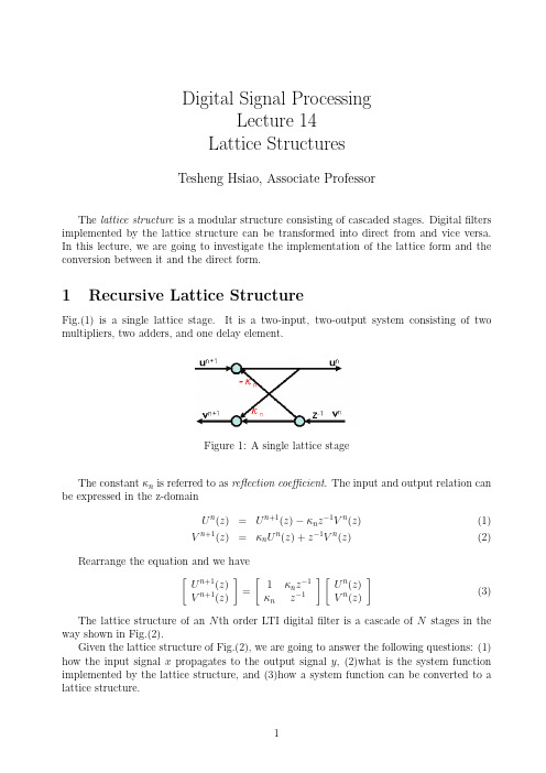
Digital Signal ProcessingLecture 14Lattice StructuresTesheng Hsiao,Associate ProfessorThe lattice structure is a modular structure consisting of cascaded stages.Digital ﬁlters implemented by the lattice structure can be transformed into direct from and vice versa.In this lecture,we are going to investigate the implementation of the lattice form and the conversion between it and the direct form.1Recursive Lattice StructureFig.(1)is a single lattice stage.It is a two-input,two-output system consisting of two multipliers,two adders,and one delayelement.Figure 1:A single lattice stageThe constant κn is referred to as reﬂection coeﬃcient .The input and output relation can be expressed in the z-domainU n (z )=U n +1(z )−κn z −1V n (z )(1)V n +1(z )=κn U n (z )+z −1V n (z )(2)Rearrange the equation and we have[U n +1(z )V n +1(z )]=[1κn z −1κn z −1][U n (z )V n (z )](3)The lattice structure of an N th order LTI digital ﬁlter is a cascade of N stages in the way shown in Fig.(2).Given the lattice structure of Fig.(2),we are going to answer the following questions:(1)how the input signal x propagates to the output signal y ,(2)what is the system function implemented by the lattice structure,and (3)how a system function can be converted to a lattice structure.Figure2:Recursive lattice structure•Lattice FilteringThe output of the lattice structure can be calculated in a recursive way.Assume that the system is at initial rest;hence v n[−1]=0,n=0,1,···,N−1.From Fig.(2),for each time step k≥0,we haveinitial conditions:v n[−1]=0,n=0,1,···,N−1for k=0,1,2,···u N[k]=x[k]for n=N−1to0u n[k]=u n+1[k]−κn v n[k−1]v n+1[k]=κn u n[k]+v n[k−1]endv0[k]=u0[k]y[k]=N∑n=0λn v n[k]end•The system function of the lattice structureLetP n(z)=U n(z)U0(z),Q n(z)=V n(z)V0(z),n=0,1,2,···,NHence,Eq.(3)can be rewritten as[P n+1(z) Q n+1(z)]=[1κn z−1κn z−1][P n(z)Q n(z)],n=0,1,2,···,N−1(4) =[1κnκn1][P n(z)z−1Q n(z)],n=0,1,2,···,N−1(5)Note thatU0(z)=V0(z),P0(z)=Q0(z)=1,X(z)U0(z)=P N(z),Y(z)U0(z)=N∑n=0λn Q n(z)Therefore the system function H (z )isH (z )=Y (z )X (z )=∑N n =0λn Q n (z )P N (z )(6)If we expand Eq.(4),we obtain [P n (z )Q n (z )]=[1κn −1z −1κn −1z −1]···[1κ0z −1κ0z −1][11],n =0,1,···,N (7)It is clear from Eq.(7)that P n (z )and Q n (z )are polynomials of z −1of order n .From Eq.(6),P N (z )is the denominator of H (z )while ∑N n =0λn Q n (z )is the numerator ofH (z ).Note that the number of parameters in the lattice structure (κn ,n =0,···N −1and λn ,n =0,···,N )is the same as the number of coeﬃcients of an N th order rational function.In summary,the system function H (z )can be determined by applying Eq.(4)recur-sively to ﬁnd P n (z )and Q n (z ),n =1,2,···,N ,given Q 0(z )=P 0(z )=1.Then use Eq.(6)to determine H (z ).•Convert the direct form to the lattice structureLet P n (z )=p n 0+p n 1z −1+···+p n n z−n and Q n (z )=q n 0+q n 1z −1+···+q n n z −n ;From Eq.(7),we have [P 1(z )Q 1(z )]=[1κ0z −1κ0z −1][11]=[1+κ0z −1κ0+z −1][P 2(z )Q 2(z )]=[1κ1z −1κ1z −1][1+κ0z −1κ0+z −1]=[1+(κ0+κ0κ1)z −1+κ1z −2κ1+(κ1κ0+κ0)z −1+z −2]...=...Hence we conclude by induction that p n n =κn −1and q n n =1for n =0,1,2,···,N .Moreover we have the following lemma.Lemma 1Q n (z )=z −n P n (z −1),n =0,1,···,NProof:This lemma can be proved by induction.The n =0case is trivialFor n =1,P 1(z )=1+κ0z −1and Q 1(z )=κ0+z −1.Thus the equality holds.Suppose that the equality holds for n =k ,i.e.Q k (z )=z −k P k (z −1).Equivalently,z −k Q k (z −1)=P k (z )For n =k +1,from Eq.(4)we haveP k +1(z )=P k (z )+κk z −1Q k (z )Q k +1(z )=κk P k (z )+z −1Q k (z )Thereforez −(k +1)P k +1(z −1)=z −k −1P k (z −1)+κk z −k Q k (z −1)=z −1Q k (z )+κk P k (z )=Q k +1(z )Thus,by mathematical induction Q n (z )=z −n P n (z −1)for n =0,1,···,NQ.E.D.Assume that κn =1for all n .If we inverse Eq.(5),we have[P n (z )z −1Q n (z )]=11−κ2n[1−κn −κn 1][P n +1(z )Q n +1(z )],n =0,1,···,N −1Hence,P n(z )=P n +1(z )−κn Q n +1(z )1−κ2n ,n =N −1,N −2,···,0(8)Let H (z )=B (z )A (z )=∑N n =0b n z −n 1−∑N n =1a n z −n ,where A (z )andB (z )are polynomials of z −1.Since p n n =κn −1for all n ,thereﬂection coeﬃcients κn ’s can be determined recur-sively by ﬁrst setting P N (z )=A (z )and Q N (z )=z −N P N (z −1).Then κN −1=p N N is determined.Applying Eq.(8)and Lemma 1recursively to ﬁnd P n (z ),κn ’s can be determined successively.To determine λn ,we observe that the coeﬃcient of z −N in the numerator must beλN since B (z )=∑Nn =0λn Q n (z )and q N N =1.Therefore λN =b N .We can removeλN Q N (z )from B (z ),resulting in a (N −1)th order polynomial,and determine λN −1by taking advantage of the property q n n =1for all n .The whole process continuous until all λn ’s are determined.In summaryP N =A (z ),S N =B (z ),λN =b Nfor n =N −1to 0κn =p n +1n +1Q n +1(z )=z −(n +1)P n +1(z −1)P n (z )=P n +1(z )−κn Q n +1(z )1−κ2nS n (z )=S n +1(z )−λn +1Q n +1(z )λn =s n nend•Stability of the Lattice Structure Form Eq.(4),we haveP 1(z )=1+κ0z −111is stable if and only if |κ0|<1.Since the lattice structure is a cascade of N similar stages,the stability of the ﬁlter can be veriﬁed easily as follows.Lemma 2The lattice structure in Fig.(2)is stable if and only if |κn |<1for all n .2All-pole SystemsAn all-pole system has no nonzero zeros,i.e.the system function is H (z )=1A (z ).In thelattice structure in Fig.(2),if λ0=1and λn =0for n >0,thenH (z )=∑N n =0λn Q n (z )P N (z )=1P N (z )Hence the all-pole system has a simpler lattice structure shown in Fig.(3).Figure 3:The lattice Structure for an all-pole systemOne interesting feature of the lattice structure in Fig.(3)is that the system function from x to v N is an all-pass system.This can be seen as follows.H all (z )=V N (z )X (z )=Q N (z )P N (z )=z −N P N (z −1)P N (z )If z 0is a pole of H all (z ),then 1/z 0must be a zero of H all (z )and vice versa.Due to the symmetry of poles and zeros,H all (z )is indeed an all-pass system.3Nonrecursive lattice structureIf H (z )=B (z ),i.e an FIR ﬁlter,the lattice structure becomes nonrecursive.We will explore its properties in this section.We would like to maintain the symmetric structure in Fig.(2)or Fig.(3)because previous results (e.q.Lemma 1)can be applied directly by doing so.In other words,Eq.(1)and Eq.(2)must hold for each stage.If H (z )is FIR,then G (z )=H −1(z )is an all-pole system.If we implement the all-pole system G (z )in the lattice form of Fig.(3),we haveG (z )=1H (z )=1P N (z )=U 0(z )U N (z )By exchanging its input and output,we get the desired FIR system.Note that in this FIR lattice structure,signals ﬂow from u 0to u N .Hence Eq.(3)should be used to compute the signal propagation from stage to stage.The corresponding lattice structure is shown in Fig.(4).Notice that the structure is nonrecursive.The system function implemented by the nonrecursive lattice structure can be constructed in the same way as the recursive lattice structure:P 0(z )=Q 0(z )=1for n =1to N [P n (z )Q n (z )]=[1κn −1z −1κn −1z −1][P n −1(z )Q n −1(z )]endH(z)=P N(z)Figure4:Nonrecursive Lattice StructureTo convert from a system function to the nonrecursive lattice structure,the algorithm is similar to that of the recursive version:P N=B(z)=1+b1z−1+···+b N z−Nfor n=N to1κn−1=p nnQ n(z)=z−n P n(z−1)P n−1(z)=P n(z)−κn−1Q n(z)1−κ2n−1endNote that from Lemma1,p n0=q nn=1for all n.Therefore the coeﬃcient of the constantterm in H(z),i.e.b0,must be1.If b0=1,an intuitive approach is to divide B(z)by b0. However,if b N=b0,as in the case of the linear phaseﬁlter,this will result inκN−1=1, and again we will run into trouble in computing the reﬂection coeﬃcients.A preferable way is to implement the FIR system H′(z)=1+(B(z)−b0)in a lattice structure and subtract 1−b0from its output.The idea is shown in Fig.(5)Figure5:Nonrecursive lattice structure for b0=1If we apply Lemma2to the nonrecursive lattice structure,we observe that B(z)is a minimum phase system if and only if|κn|<1for all n.If B(z)=P N(z)is a minimum phase system,then the system function from x=u0to v N,i.e.Q N(z),becomes a maximum phase system according to Lemma1,i.e.all its zeros are outside the unit circle.Aﬁnal remark of this lecture:According to Lemma2,each stage of the stable(or minimum phase)lattice structure is an attenuator,i.e.it does not amplify the signals.Thisproperty gives the lattice structure great computational stability and this is the primary reason that the lattice structure is implemented.However,the price for this property is the complex computation of the signalﬂow.。

Cartographic objects in a multi-scale data structure

Cartographic objectsin a multi-scale data structureSabine TimpfDept. for GeoinformationTechnical University ViennaGusshausstr. 27-29, A - 1040 Viennatimpf@geoinfo.tuwien.ac.atABSTRACTGIS need a function to draw sketches quickly and in arbitrary scales. We propose a multi-scale hierarchical spatial model for cartographic data. Objects are stored with increasing detail and can be used to compose a map at a particular scale. This results in a multi-scale cartographic forest when applied to cartographic mapping. The structure of the multi-scale forest is explained. It is based on a trade-off between storage and computation. Methods to select cartographic objects for rendering are based on the principle of equal information density.1. INTRODUCTIONGeographic Information Systems manage data with respect to spatial location and those data are presented graphically as a map or sketch. There are a number of similar graphics applications, where a database of entities with some geometric properties is used to render these entities graphically for different tasks. Typically these tasks require graphical representations at different levels of detail, ranging from overview screens to detailed views1Timpf, S. 1997. "Cartographic objects in a multi-scale data structure". In Geographic Information Research: Bridging the Atlantic. (Craglia, M., & Couclelis, H., eds.), 1 vols., Vol. 1, London,Taylor&Francis, pp: 224-234.(Herot et al., 1980). A function to draw cartographic sketches quickly and in arbitrary scales is needed. In practical applications, a base map is stored and its scale changed graphically. Without major distortions, only changes to twice or half the original scale are feasible by simple numeric scale change. This calls for map generalization, a notoriously difficult problem. Efforts to achieve automated cartographic generalization were successful for specific aspects (Freeman, and Ahn, 1987; Powitz, 1993; Staufenbiel, 1973), but no complete solution is known, nor are any to be expected within the immediate future. Buttenfield and McMaster give a comprehensive account of the current research trends (Buttenfield and McMaster, 1991).1.1 MotivationDisplays should be more adaptable to users needs and their tasks instead of creating and presenting a static view of the data (Lindholm and Sarjakoski, 1994). In current approaches, objects to render are selected for each map and then transformed into cartographic objects to construct a map. This conforms to the traditional view of the cartographic process (Fig. 1). Generalization is done each time a new map is constructed and each time a new selection of the entities to display is performed. The term ’entities’ refers to the things in the world, whereas the term ’objects’ refers to things in the database.Figure 1: Traditional view of the cartographic process The simplification we propose is to transform the entities just once into cartographic objects. We assume that geographic objects have a slow change rate and that the database is updated in appropriate intervals. The cartographic objects are stored at multiple scales in a single database (Beard, 1987) from which they are selected for each map output (Fig. 2).This database will not be much larger than the most detailed database assumed in current proposals (assume that every generalized representation is a quarter of the size of theprevious one, then the total storage requires only one third more capacity than the most detailed data set). Generalized representations can be collected from existing maps or for some cases produced automatically. A similar approach has already been presented by van Oosterom (Van Oosterom, 1989), who proposed to use an R-tree for storage of the generalized objects. Our approach is broader, in that we model the underlying conceptual organization of cartographic objects in a map and are not yet concerned with implementation methods.Figure 2: Selection processThe data structure chosen is a multi-scale cartographic forest, where renderings for objects are stored at different levels of detail. A forest is a collection of trees and therefore essentially a directed acyclic graph (DAG). This extends ideas of hierarchies or pyramids and is related to quad-trees (Samet, 1989b) and strip-trees (Ballard, 1981). The structure of the multi-scale forest is based on a trade-off between storage and computation, replacing all steps which are difficult to automate by redundant storage. The resulting forest structure is more complex than the hierarchical structures proposed in the literature so far (Samet,1989a; Samet, 1989b). Objects may change their appearance considerably, for example, they change their spatial dimension, or change from a single object to a group of objects. Special attention requires the case when new objects appear when we zoom in or disappear when we zoom out. In this work we will consider the operation zooming as a new perspective on the problem of multi-scale representations. We are convinced that the results will have an impact on the problem of generalization. The multi-scale structure will also support multi-level modeling and combinations of objects in different scales in one map as introduced in Bullen (1995).From the database, the map output is constructed as a top-down selection of pre-generalized cartographic objects, until a sufficient level of detail is achieved. Pre-generalized cartographic objects can be taken from existing map series. The dominant operation is ’zoom,’ intelligently replacing the current graphical representation with a more detailed one, that is appropriate for the selected new scale. Methods to select objects for rendering are based on the principle of equal information density, which can be derived from Töpfer's radix law (Töpfer and Pillewitzer, 1966) and has been used by cartographers (Beck, 1971). We propose a relatively simple method to achieve equal information density, namely measuring 'ink'.1.2 Structures of geographic objectsThere are several types of geographic objects in the world. Couclelis (Couclelis, 1994) made the distinction between objects and entities (Fig. 3). Entities are things in the real world that we can perceive. In our representation (our mental model) entities become objects: representations of things in the real world.Most geographic objects do not have directly visible and sharp boundaries (geological layers, soils); others do not have visible boundaries but boundary zones or undetermined boundaries (e.g., forest, sand dunes) (Burrough and Frank, 1995).There are two views (or models) of the world which have impact on the data structure chosen. The field view sees the world as a continuum and therefore implies that there are no real boundaries unless we define them. The object view divides the world into objects with different properties and sharp boundaries. Both views have their advantages and their drawbacks. We will try to incorporate both views in our data structure, although traditionalpaper maps adhere to the object view of the world. Pantazis proposed a conceptual framework in which both views coexist (Pantazis, 1995). Unfortunately the classes in his framework cannot be used for a classification of graphical objects to be used for our approach.2. A MULTI-SCALE STRUCTUREOne approach for structuring cartographic data is to consider cartography as a language with its own syntax and vocabulary (Palmer and Frank, 1988; Robinson and Petchenik, 1976; Youngmann, 1977). These objects are combined from a graphical vocabulary, which provides the atoms for graphical communication (Bertin, 1967; Head, 1991; Mackinlay, 1986; Schlichtmann, 1985). Highly simplified, cartographic objects can be differentiated by dimension (points, lines, areas) and the cartographic variations (object drawn as symbol, object representing a scaled representation, a feature associated with text, and text without a delimited graphical feature). This results in a dozen geometric categories (Morrison, 1988).The approach selected here is to construct a multi-scale directed acyclic graph (DAG) for each semantic class that exists in a map and to specify rules for their interaction. Semantic classes are waterbodies, railroads, roads, settlements, labels, and symbols (Hake, 1975; Staufenbiel, 1973). They represent the first stage in a characterization of object features which roughly corresponds to first level conceptual groups humans have. The second stage will be realized through the 12 categories mentioned above. We will have to examine the feasibility of this approach.2.1 Data structureThe idea is that every entity is represented at multiple scales (Buttenfield and Delotto, 1989) in a forest, i.e., there are multiple graphical renderings for every cartographic object, organized in increasing graphical detail and pre-generalized. This includes that an object may split in sub-objects, each with its own graphical rendering (Fig. 4). Generalizedrepresentations can be collected from existing map series or, for some cases, produced automatically. This circumvents cartographic generalization at the expense of storage.In Figure 4, a multi-scale DAG for houses is shown. At a very high level (meaning small-scale) the graphical object ’house’ is not rendered at all, at a lower level it is rendered as a symbol, then as a generalized geometrical representation, and as a geometrical description.Between each of these renderings a jump in the representation method is made.In the next lower level, the geometry is depicted more clearly and it is shown that the object is, in fact, an aggregated object, and the representation method remains the same. The most detailed rendering is again made possible through a jump in the representation method.These jumps correspond to special operations of the zooming process, e.g. specialization and disaggregation.1: 50 0001: 25 0001: 10 0001: 5 0001: 10001: 100 0001: 500 000Considering existing map series, where the same objects are mapped at different scales, a strategy for hierarchization follows (Table 1). The list demonstrates that objects may change their spatial dimension in the generalization hierarchy. A particular problem is posed by objects which are not represented at small scale and seem to appear as one zooms in. Thisappearance of objects can be accounted for in the indexing data structure which will again be a graph.Table 1: Types of changes of object representations for smaller to larger scaleMost of the change types (1-4, 6,7 in Table 1) are not reflected in the data structure (Fig. 5a).no changeincrease of scalechange in symbolincrease of setailchange in dimensionshift to geometric formFig. 5a: Examples for the changes, that do not affect the data structure However, change types 5, 8, and 9 affect the data structure. The change types‘appearance of a label’ and ‘object appears’ require a new link to come into the existing DAG from the outside (Fig. 5b).y(n o gFig. 5b: Examples for the change types ’appearance of label’ and ’object appears’The change type ‘split into several objects’ requires that more than one link is leading from a single node (Fig. 5c)....Fig. 5c: Example for the change type 'split into several objects' Of these two structural change types, namely new link and several links from one node, the first is the more important one and also the most difficult to handle.2.2 Why a Directed Acyclic Graph?A directed acyclic graph (DAG) is a well known and documented structure in graph theory (Perl, 1981) and it has many applications in the database area (Güting, 1994). The logical data structure suited for zooming would be one that links object representations of one level or scale with object representations of another level or scale in a hierarchical fashion. In our structure the nodes of the DAG contain the object representations and therefore the information necessary to render the objects. The directed links determine the direction of the zooming-in process.In graph theory a forest is a collection of trees while trees are acyclic graphs (Ahuja, Magnanti, and Orlin, 1993; Perl, 1981). In our data structure each object group (waterbodies, railroads, roads, settlements, labels, and symbols) is represented by a forest (Fig. 6). E.g., a number of houses at a certain location on the map can build a single tree because of their spatial proximity. Houses in a different area of the map build a second tree, and so forth. All 'house-trees' combined thus build a forest. This is true for all object groups. The whole collection of forests is again a forest. The forest contains the information for rendering in the nodes and the information for selection on the links.When implementing the structure we use an approach similar to the Reactive Tree (Van Oosterom, 1989). The difference is that we first classify the graphical objects and construct several trees that are spatially intertwined. They may then be represented in a reactive tree. There is still research to be done to define the relationships between the different trees and forests in order to preserve topology between objects from different groups.3. 3. MOVING ABOUT IN THE STRUCTUREZooming is a concept that originates from the metaphor of the sound of an airplane flying towards the earth. This means that as we get nearer to the object of interest, we see more detail. In computer graphics this has been partly realized as getting nearer to the focus of the window of interest while enlarging the information contained in the window (Fig. 7a). Volta (1992) studied a content zoom in which the categories of the window of interest are shown in more detail (Fig. 7b). For example, three major soil classes are differentiated into a detailed schema of several dozen classes. We identified the need for an intelligent zoom (Frank and Timpf, 1994), that realizes both requirements for zooming (Fig. 7c).Figure 7a: A graphical zoomFigure 7c: An intelligent zoomBy intelligent zoom we understand a zoom operation, which respects the known principle of equal information density (Beck, 1971; Töpfer and Pillewitzer, 1966). It implies that more detail about objects become visible as the field of vision is restricted and the scale is increased. This leads immediately to a hierarchical data structure, where objects are gradually subdivided in more details. This hierarchical structure is applied to all geometric objects, not only to lines as in strip trees (Ballard, 1981) or in the model of Plazanet (1995), to a pixel representation of an area as in a quadtree (Samet, 1989a; Samet, 1989b) or the pyramid structures used in image processing (Rosenfeld et al., 1982). When continuously zooming, the jumps in representations could be smoothed by using a morphing algorithm. Literature on 2D-morphing of geometric features is abundant and well researched (see for example (Sederberg and Greenwood, 1992)).4. SELECTION CRITERIONThe problem to address is the selection of the objects in the forest which must be rendered. Two aspects can be separated, namely, the selection of objects which geometrically extend into a window and the selection of objects to achieve constant information density. The selection of objects which extend into the window is based on a minimal bounding rectangle for each object and a refined decision that can be made based on object geometry. In order to assure fast processing in the multi-scale forest, the minimal bounding rectangles must be associated with the forest and forest branching, such that complete sub-forests can be excluded based on window limits. This is well known and the base for all data structures which support fast spatial access (Samet, 1989a; Samet, 1989b).The interesting question is how the depth of descent into the forest is controlled to achieve equal information density. In data structures for spatial access, an ’importance’characteristic has been proposed (Van Oosterom, 1989). It places objects which are statistically assessed as important higher in the forest and they are then found more quickly. The method relies on an assessment of the ’importance’ of each object, which is done once when the object is entered into the cartographic database. When a cartographic sketch is desired, the most important objects are selected for rendering from this ordered list. The usability of this idea is currently studied for a particular case, namely the selection of human dwellings (cities) for inclusion in a map (Flewelling and Egenhofer, 1993). A method based on an ordering of objects is not sufficient for the general case.The cartographic process is fundamentally constrained by the limit, that one piece of paper can carry only one graphical message. The cartographic selection process is mostly dealing with the management of the resource map space and how it is allocated. The graphical density of the displays should be preserved over several scales.A relatively simple practical method for uniform graphical density is to measure ’ink’, i.e., pixels which are black. One assumes then that there is a given ratio of ink to paper. This ratio must be experimentally determined, measuring manually produced good maps (e.g., 1 inked cell per 10 cells of paper). The expansion of the forest involves progressing from the top to the bottom, accumulating ink content and stopping when the preset value for graphical density is reached. The ink content should not be measured for the full window, but the window should be subdivided and ink for each subdivision optimized. We have not yet found a suitable method for subdividing the window and optimizing the ink content.This selection principle does not avoid that two objects can be rendered at the same location. It requires afterwards a placement process (similar in kind to the name placement algorithm known) to assign a position to each object (Herot et al., 1980). It also requires a method for displacement of objects as proposed in e.g. (Bundy, Jones, and Furse, 1994).5. CONCLUSIONSA number of applications require graphical presentations of varying scale, from overview sketches to detailed drawings. A simple scale change is not sufficient to produce drawings which humans can easily understand. The problem is most visible in cartographic mapping, where map scales vary from 1:1,000 to 1:100,000,000, covering a range of 105. Over the last five centuries, cartography has developed useful methods to produce overview maps from more detailed ones. Several complex filtering rules are used to delete what is less important, simplify the objects retained, etc. Unfortunately these rules have not been formalized and it was not possible, despite great efforts and partial solutions, to produce a fully automated system.The proposed multi-scale forest is a method to produce maps of different scales from a single database. This avoids the difficulty of cartographic generalization at the expense of storage. Objects are stored at different levels of generalization, assuming that --at least for the difficult cases-- the generalization is done by humans, but only once. Building a multi-scale forest is probably a semi-automated process where automated processes are directed by a human cartographer. All operations where valuable human time is necessary are done only once and the results are stored.The concept is based on a trade-off between computation and storage, replacing all steps which are difficult to automate with storage. These steps are performed initially, while the remaining steps, which can be easily automated, are performed each time a query asks for graphical output.The resulting forest structure is more complex than spatial hierarchical structures proposed in the literature so far, as objects may change their geometric appearance considerably. For example, they change their spatial dimension, or change from a single object to a group of objects. Special attention requires the case that objects seemingly appear as we zoom in. The proposed forest is related to quad-tree or strip-tree structures, but generalized: objects of all dimensions can be stored and the dimension of an object between steps of generalization can change.One of the problems encountered in this study is the small body of literature on cartographic formalization. We think, that more studies are needed in the formalization of cartographic knowledge and in cartographic theories.ACKNOWLEDGMENTSI thank Werner Kuhn and Andrew Frank for their inspiring discussions on this topic. I also thank all participants of the summer institute for their good comments on my presentation. Finally I thank the anonymous reviewers for their detailed comments.REFERENCESAhuja, R. K., Magnanti T. L., and Orlin, J. B., 1993, Network Flows: Theory, Algorithms, and Applications, (Englewood Cliffs, NJ: Prentice Hall).Ballard, D. H., 1981, Strip Trees: A Hierarchical Representation for Curves. ACM Communications, 24, (5), pp. 310-321.Beard, K., 1987, How to survive on a single detailed database. In: Auto-Carto 8 in Baltimore, MA, edited by N. R. Chrisman, (ASPRS & ACSM), pp. 211-220.Beck, W., 1971, Generalisierung und automatische Kartenherstellung. Allgemeine Vermessungs-Nachrichten, 78 (6), pp. 197-209.Bertin, J., 1967, Sémiologie Graphique, (Gauthier-Villars).Bullen, N., 1995, Linking GIS and Multilevel Modelling in the Spatial Analysis of House Prices. In this volume (Taylor & Francis).Bundy, G.Ll., Jones, C.B., and Furse, E., 1994, A topological structure for the generalization of large scale cartographic data. In: GISRUK, Leicester, England, edited by P. Fisher, pp.87-96.Burrough, P., and Frank, A. U., 1995, Natural Objects with Indeterminate Boundaries, GISDATA Series, (Taylor and Francis) (in press).Buttenfield, B.P., and McMaster, R., 1991, Rule based cartographic generalization, (London: Longman).Buttenfield, B.P., and Delotto, J., 1989, Multiple Representations: Report on the Specialist Meeting. National Center for Geographic Information and Analysis, Santa Barbara, CA, Report 89-3.Couclelis, H., 1994, Towards an operational typology of geographic entities with ill-defined boundaries, TU Wien, Position paper at the Workshop on objects with undeterminate boundaries.Flewelling, D. M., and Egenhofer, M. J., 1993, Formalizing Importance: Parameters for Settlement Selection. In: 11th International Conference on Automated Cartography, Minneapolis, MN, (ACSM).Frank, A. U., and Timpf, S., 1995, Multiple representations for cartographic objects in a multi-scale tree - An intelligent graphical zoom. Computers and Graphics Special issue: Modelling and Visualisation of Spatial Data in Geographical Information Systems, 18(6), pp. 823-830.Freeman, H., and Ahn, J., 1987, On the Problem of Placing Names in a Geographic Map.International Journal of Pattern Recognition and Artificial Intelligence, 1 (1), pp. 121-140.Güting, R.H., 1994, GraphDB: A Data Model and Query Language for Graphs in Databases.FernUniversität Hagen, Informatik-Bericht 155.Hake, G., 1975, Kartographie. (Göschen/de Gruyter).Head, C. G., 1991, Mapping as language or semiotic system: review and comment. In Cognitive and Linguistic aspects of space, editde by D.M. Mark and A.U. Frank,(Dordrecht: Kluwer Academic Publishers), pp. 237-262.Herot, C.F. et al., 1980, A Prototype Spatial Data Management System. Computer Graphics,14 (3).Lindholm, M. and Sarjakoski, T., 1994, Designing a visualization user interface. In Visualization in modern cartography, edited by A. MacEachren and D.R.F. Taylor, (Oxford: Pergamon, Elsevier Science Ltd.), pp. 167-184.Mackinlay, J., 1986, Automating the Design of Graphical Presentations of Relational Information. Transactions on Graphics, 5 (2), pp. 110-141.Morrison, J., 1988, The proposed standard for digital cartographic data. American Cartographer, 15 (1), pp. 9-140.Palmer, B. and Frank, A., 1988, Spatial Languages. In: Third International Symposium on Spatial Data Handling, Sydney, Australia, edited by D. Marble, pp. 201-210. Pantazis, D., 1995, CON.G.O.O., a conceptual formalism for geo-graphic models: basic concepts and extensions for modeling of objects with indeterminate boundaries. In this volume, (Taylor & Francis) (in press).Perl, J., 1981, Graph Theory (in german). (Wiesbaden (FRG): Akademische Verlagsgesellschaft).Plazanet, C., 1995, Geometry modeling for linear feature generalization. In this volume, (Taylor & Francis) (in press).Powitz, B.M., 1993, Zur Automatisierung der kartographischen Generalisierung topographischer Daten in Geo-Informationssystemen. PhD-thesis, University ofHannover.Robinson, A.H., and Petchenik, B.B., 1976, The Nature of Maps: Essays toward Understanding Maps and Mapping. (Chicago: The University of Chicago Press). Rosenfeld, A. et al., 1982, Applications of hierachical data structures to geographical information systems. Computer Vision Laboratory, Computer Science Center, University of Maryland.Samet, H., 1989a, Applications of Spatial Data Structures: Computer Graphics, Image Processing and GIS. (Reading, MA: Addison-Wesley).Samet, H., 1989b, The Design and Analysis of Spatial Data Structures. (Reading, MA: Addison-Wesley).Schlichtmann, H.,1985, Characteristic traits of the semiotic system ’map symbolism’.Cartographic Journal, pp. 23-30.Sederberg, T.W., and Greenwood, E., 1992, A physically shaped approach to 2-D shape blending. In: Computer Graphics Proceedings SIGGRAPH’92 edited by SIGGRAPH, ACM, (Addison-Wesley), pp. 25-34.Staufenbiel, W., 1973, Zur Automation der Generalisierung topographischer Karten mit besonderer Berücksichtigung grossmasstäbiger Gebäudedarstellungen. Kartographisches Intitut Hannover. Wissenschaftliche Arbeiten WissArbUH 51.Töpfer, F., and Pillewitzer, W., 1966, The principes of selection.” Cartographic Journal, (3), pp. 10-16.Van Oosterom, P., 1989, A reactive data structure for geographic information systems. In: Auto-Carto 9, Baltimore, MA, edited by E. Anderson, (ASPRS & ACSM), pp. 665-674. Volta, Gary., 1992, Interaction with attribute data in Geographic Information Systems: A model for categorical coverages. Master of Science, University of Maine, USA. Youngmann, Carl., 1977, A linguistic approach to map description. In: First International Advanced Study Symposium on Topological Data Structures for Geographic Information Systems, Cambridge, Mass., edited by G. Dutton, Laboratory for Computer Graphics and Spatial Analysis, Harvard University, pp.1-17.。

data structure +课程内容

英文回答：The concept of data structure is a fundamental and essential element in the field ofputer science, with a primary focus on the organization and storage of data in a manner that facilitates efficient access and manipulation. It constitutes a criticalponent in the development of effective algorithms and significantly influences the performance of software applications. The study of data structure epasses an in-depth understanding of various types of data structures, including arrays, linked lists, stacks, queues, trees, graphs, and others. Proficiency inprehending the characteristics, operations, and applications of these data structures is indispensable for individuals involved in programming or software development. Within the framework of aputer science curriculum, students engage in learning the principles and methodologies of data structure design and implementation, as well as conducting thorough analysis of their efficiency and performance across diverse applications.数据结构的概念是计算器科学领域的一个基本要素，主要侧重于以有利于高效获取和操纵的方式组织和储存数据。

AUGMENTEDQUAD-EDGE–3DDATASTRUCTURE…

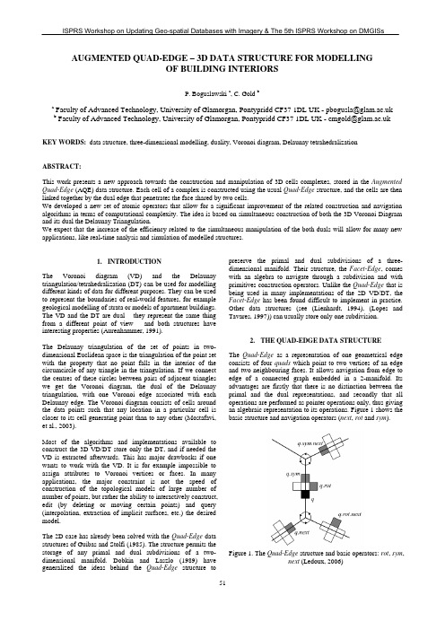
AUGMENTED QUAD-EDGE – 3D DATA STRUCTURE FOR MODELLINGOF BUILDING INTERIORSP. Boguslawski a, C. Gold ba FacultyofAdvancedTechnology,UniversityofGlamorgan,************************************.ukb FacultyofAdvancedTechnology,UniversityofGlamorgan,**********************************.uk KEY WORDS: data structure, three-dimensional modelling, duality, Voronoi diagram, Delaunay tetrahedralizationABSTRACT:This work presents a new approach towards the construction and manipulation of 3D cells complexes, stored in the Augmented Quad-Edge (AQE) data structure. Each cell of a complex is constructed using the usual Quad-Edge structure, and the cells are then linked together by the dual edge that penetrates the face shared by two cells.We developed a new set of atomic operators that allow for a significant improvement of the related construction and navigation algorithms in terms of computational complexity. The idea is based on simultaneous construction of both the 3D Voronoi Diagram and its dual the Delaunay Triangulation.We expect that the increase of the efficiency related to the simultaneous manipulation of the both duals will allow for many new applications, like real-time analysis and simulation of modelled structures.1.INTRODUCTIONThe Voronoi diagram (VD) and the Delaunay triangulation/tetrahedralization (DT) can be used for modelling different kinds of data for different purposes. They can be usedto represent the boundaries of real-world features, for example geological modelling of strata or models of apartment buildings. The VD and the DT are dual – they represent the same thing from a different point of view – and both structures have interesting properties (Aurenhammer, 1991).The Delaunay triangulation of the set of points in two-dimensional Euclidean space is the triangulation of the point set with the property that no point falls in the interior of the circumcircle of any triangle in the triangulation. If we connect the centres of these circles between pairs of adjacent triangles we get the Voronoi diagram, the dual of the Delaunay triangulation, with one Voronoi edge associated with each Delaunay edge. The Voronoi diagram consists of cells around the data points such that any location in a particular cell is closer to its cell generating point than to any other (Mostafavi,et al., 2003).Most of the algorithms and implementations available to construct the 3D VD/DT store only the DT, and if needed the VD is extracted afterwards. This has major drawbacks if one wants to work with the VD. It is for example impossible to assign attributes to Voronoi vertices or faces. In many applications, the major constraint is not the speed of construction of the topological models of large number of number of points, but rather the ability to interactively construct, edit (by deleting or moving certain points) and query (interpolation, extraction of implicit surfaces, etc.) the desired model.The 2D case has already been solved with the Quad-Edge data structures of Guibas and Stolfi (1985). The structure permits the storage of any primal and dual subdivisions of a two-dimensional manifold. Dobkin and Laszlo (1989) have generalized the ideas behind the Quad-Edge structure to preserve the primal and dual subdivisions of a three-dimensional manifold. Their structure, the Facet-Edge, comes with an algebra to navigate through a subdivision and with primitives construction operators. Unlike the Quad-Edge that is being used in many implementations of the 2D VD/DT, the Facet-Edge has been found difficult to implement in practice. Other data structures (see (Lienhardt, 1994), (Lopes and Tavares, 1997)) can usually store only one subdivision.2.THE QUAD-EDGE DATA STRUCTUREThe Quad-Edge as a representation of one geometrical edge consists of four quads which point to two vertices of an edge and two neighbouring faces. It allows navigation from edge to edge of a connected graph embedded in a 2-manifold. Its advantages are firstly that there is no distinction between the primal and the dual representations, and secondly that all operations are performed as pointer operations only, thus giving an algebraic representation to its operations. Figure 1 shows the basic structure and navigation operators (next, rot and sym).Figure 1. The Quad-Edge structure and basic operators: rot, sym,next (Ledoux, 2006)3. AUGMENTED QUAD-EDGE (AQE)The AQE (Ledoux and Gold, in press), (Gold, et al., 2005) uses the Quad-Edge to represent each cell of a 3D complex, in either space. For instance, each tetrahedron and each Voronoi cell are independently represented with the Quad-Edge , which is a boundary representation. With this simple structure, it is possible to navigate within a single cell with the Quad-Edge operators, but in order to do the same for a 3D complex two things are missing: a ways to link adjacent cells in a given space, and also a mechanism to navigate to the dual space. In this case two of the four org pointers are not used in 3D. The idea is to use the free face pointers in the Quad-Edge to link two cells sharing a face. This permits us to link cells together in either space, and also to navigate from a space to its dual. Indeed, we may move from any Quad-Edge to a Quad-Edge in the dual cell complex, and from there we may return to a different cell in the original cell complex.The AQE is high in storage but it is computationally efficient (Ledoux, 2006). Each tetrahedron contains 6 edges – each one is represented by four quads containing 3 pointers. This makes a total of 72 pointers. The total number of pointers for the dual is also 72. It makes a total of 144 pointers for each tetrahedron. However we preserve valuable properties which are crucial in real-time computations.Construction and navigation In previous work the theoretical basis of the storage and manipulation of 3D subdivisions with use of the AQE were described (Ledoux and Gold, in press) and it was shown that this model worked.The main construction operator is MakeEdge . It creates a single edge, that at the moment of creation it is not linked to any other edge. The Splice operator is used to link edges in the same subdivision. Edges in the dual subdivisions are linked one-by-one later using the through pointer.a)b)Figure 2. Flip operators (Ledoux, 2006): a) flip14 is used when a new point is inserted. Its reverse is flip41; b) flip23 is used when the structure has to be modified in order to preserve thecorrect DT. Its reverse is flip32.When a new point is inserted in the structure of the DT, four new tetrahedra are created inside the already existing one that contains the newly inserted point. Then the enclosing tetrahedron is removed. The new corresponding Voronoi points are calculated and another tetrahedron is created separately in the dual subdivision. Then all edges are linked together and, to maintain a properly built DT structure, subdivisions are modified by flip operators. Two basic flip operators are shown in Figure 2.Another requirement for the navigation is the through pointer that links together both dual subdivisions (Ledoux and Gold, in press), (Ledoux, 2006). The org pointers that are not used in 3D allow for making a connection to the dual edge. With this operator it is possible to go to the dual subdivision and back to the origin. It is the only way to connect two different cells in the same subdivision.Figure 3. The through pointer is used to connect both dualsubdivisions (Ledoux, 2006)To get the shared face of two cells, the adjacent operator is used. It is a complex operator that consists of a sequence of through and other basic operators. (Ledoux, 2006)4. ATOMIC OPERATORS The general algorithm of the point insertion to the DT/VD structure was described by Ledoux (2006). In our current work we have implemented and improved the way of building the whole structure.Algorithm 1: ComplexMakeEdge (DOrg, DDest, VOrg, VDest)// DOrg, DDest – points defined edge in DT // VOrg, VDest – points defined edge in VDe1:=MakeEdge(DOrg, DDest); e2:=MakeEdge(VOrg, VDest); e1.Rot.V:=e2;e2.InvRot.V:=e1.Sym;The most fundamental operator is ComplexMakeEdge which creates two edges using MakeEdge (Ledoux, 2006). They are dual and the one belongs to the DT and the second to the VD. The V pointer from the Quad-Edge structure is used to link them as shown in Algorithm 1. We claim that the connection between the newly created edges in both dual subdivisions has a very important property – it is permanent and not changed by any other operator.Algorithm 2: InsertNewPoint(N) – ComplexFflip14// N – new point inserted to the DT1.Find tetrahedron which contain point N2.Calculate 4 new Voronoi points3.Create new edges with using ComplexMakeEdge withpoint N and new Voronoi points4.Assign through pointers5.Disconnect origin edges of tetrahedron using Splice6.Connect edges of 4 new tetrahedra using Splice7.Add 4 new tetrahedra to a stack8.while necessary do flip23 or flip32 for tetrahedra fromthe stackFigure 4. fli p14 divides origin tetrahedron ABCD into 4 new The first operation in the point insertion to the structure is flip14 (Fig. 2a). It divides space occupied by tetrahedron ABCD into four smaller ones (Fig. 4). The inserted point N is a vertex shared by new tetrahedra. As mentioned above, this version of the algorithm is an improvement over Ledoux (2006). The significant aspect is that we don’t remove the origin tetrahedra and create 4 new. Edges from the origin tetrahedron are disconnected and used to create 4 new. Thus no edges are deleted from the DT structure. What is more, the same applies to the VD because dual edges are linked together permanently. Only new edges are added to the structure.Tetra- hedronEdges from originABCD tetrahedronused to create 4 newNewly created edgesT I CA, AD DC, CN, AN, DNT II AB, BD DA, AN, BN, DNT III BC, CD DB, BN, CN, DNT IV - BA, AC, CB, BN, AN, CNTable 5. Edges used in flip14Table 5 in conjunction with Fig. 2a) shows which edges are created and which ones are taken from the origin tetrahedron. The operation of point insertion does not demand any modification to the whole structure except for local changes of a single cell. This case is implemented in the ComplexFlip14 operator (Algorithm 2). The structure created this way keeps all new cells connected, and navigation between them, and within the whole structure, remains possible. The new complex operator is more efficient because it requires fewer operations to insert a point and modify the structure.Tetra-hedronEdges from origintetrahedra used tocreate new onesNewlycreatededgesDeletededgesT’ Ifrom TI: BEfrom TII: BD, ABAE, AD,DEAB (from TI) T’ IIfrom TI: AEfrom TII: AD, CACE, CD,DECA (from TI) T’ IIIfrom TI: CEfrom TII: CD, BCBE, BD,DEBC (from TI)Table 6. Edges used in flip23Algorithm 3: flip23(TI, TII):// TI, TII – two adjacent tetrahedra1.Calculate 3 new Voronoi points2.Copy edges and create new ones as shown in Table 63.Assign through pointers4.Disconnect edges of 2 original tetrahedra using Splice5.Connect edges of 3 new tetrahedra using Splice6.Remove spare edges (see Table 6)7.Remove 2 old Voronoi points8.Add 6 new tetrahedra to the stackTetra-hedronEdges from origintetrahedra used tocreate new onesNewlycreatededgesDeleted edges T Ifrom T’I: BEfrom T’II: CEfrom T’III:AEAB, BC,CAT IIfrom T’I: AB, BDfrom T’II: BC, CDfrom T’III: CA, AD-from T’I: AE,AD, DEfrom T’II: BE,BD, DEfrom T’III: CE,CD, DETable 7. Edges used in flip32Algorithm 4: flip32(TI, TII, TIII):// TI, TII, TIII – three tetrahedra adjacent in pairs1.Calculate 2 new Voronoi points2.Copy some edges and create new ones as shown inTable 73.Assign t hrough pointers4.Disconnect edges of 3 origin tetrahedra using Splice5.Connect edges of 2 new tetrahedra using Splice6.Remove spare edges (see Table 7)7.Remove 3 old Voronoi points8.Add 6 new tetrahedra to the stackFinally all edges are linked together to give a correctly built structure. Then correctness tests are performed. They check if the new tetrahedra have built the correct DT structure. If not, flip23 (Algorithm 3) or flip32 (Algorithm 4) are executed(Ledoux, 2006). Edges taking part in these operators are listed in Tables 6 and 7 and showed in Fig. 2b).To check the validity of our assumptions a special computer application was created. The implementation showed that our new complex operators work. The number of required operations for creation and deletion of edges and assignment of pointers has significantly decreased from the previous work of (Gold, et al., 2005).PUTER AIDED MODELLING Emergency planning and design of buildings are major issues for many people especially after 11th September 2001. To manage disasters effectively they need tools for rapid building plan compilation, editing and analysis.In many cases 2D analysis is inadequate for modelling building interiors and escape routes. 3D methods are needed. This is more obvious in disciplines such as geology (with complex adjacencies between rock types) and building construction (with security aspects). There is no appropriate data structure to describe those issues in a “3D GIS” context.Figure 8. The AQE is an appropriate structure for the modelling of building interiors. (Ledoux, 2006)The new operators can be used for advanced 3D modelling. In our opinion the AQE is a good structure for the modelling of building interiors (Fig. 8). Faces in the structure are stored twice, so every wall separating two rooms can have different properties on each side. It can help to make models not only of simple buildings but also of overpasses, tunnels and other awkward objects. It will be possible to create systems for disaster management, for example to simulate such phenomena as spreading fire inside buildings, flooding, falling walls, terrorist activity, etc.Another example is navigation in buildings, which requires the primal graph for forming rooms and the dual graph for making connections between rooms. Even though one can be reconstructed from the other, they both are needed for full real-time query and editing. These graphs need to be modifiable in real-time to take account of changing scenarios. This 3D Data Structure will assist applications in looking for escape routes from buildings.6.CONCLUSIONSOur current work involved the development and improvement of the atomic construction operations similar to the Quad-Edge. When we complete all atomic operators and prove their correctness, we will be able to use binary operations for location of quads in the stored structures. That will improve the efficiency of algorithms and allow for their use in real-time applications.In future work we will try to create a basic program for the modelling of building interiors and implement new functions such as the evaluation of optimal escape routes. We believe that such basis “edge algebra” has many practical advantages, and that it will be a base for many future applications.REFERENCESAurenhammer, F., 1991. Voronoi diagrams: A survey of a fundamental geometric data structure. ACM Computing Surveys, 23 (3), pp. 345-405.Dobkin, D. P. and Laszlo, M. J., 1989. Primitives for the manipulation of three-dimensional subdivisions. Algorithmica, 4, pp. 3-32.Gold, C. M., Ledoux, H. and Dzieszko, M., 2005. A Data Structure for the Construction and Navigation of 3D Voronoi and Delaunay Cell Complexes. WSCG’2005 Conference, Plzen, Czech Republic.Guibas, L. J. and Stolfi, J., 1985. Primitives for the manipulation of general subdivisions and the computation of Voronoi diagrams. ACM Transactions on Graphics, 4, pp. 74-123.Ledoux, H. and Gold, C. M., in press. Simultaneous storage of primal and dual three-dimensional subdivisions. Computers, Environment and Urban Systems.Ledoux, H., 2006. Modelling three-dimensional fields in geoscience with the Voronoi diagram and its dual. Ph.D. dissertation, School of Computing, University of Glamorgan, Pontypridd, Wales, UK.Lienhardt, P., 1994. N-dimensional generalized combinatioral maps and cellular quasi-manifolds. International Journal of Computational Geometry and Applications, 4 (3), pp. 275-324. Lopes, H. and Tavares, G., 1997. Structural operators for modelling 3-manifolds. Proceedings 4th ACM Symposium on Solid Modeling and Applications, Atlanta, Georgia, USA, pp. 10-18.Mostafavi, M. A., Gold, C. M. and Dakowicz, M., 2003. A Delete and insert operations in Voronoi/Delaunay methods and applications. Computers & Geosciences, 29 (4), pp. 523-530.。

Geometric Modeling

Geometric ModelingGeometric modeling is a crucial aspect of computer graphics and design, playing a significant role in various fields such as engineering, architecture, animation, and gaming. It involves the creation and manipulation of geometric shapes and structures in a digital environment, allowing for the visualization and representation of complex objects and scenes. However, despite its importance, geometric modeling presents several challenges and limitations that need to be addressed in order to improve its efficiency and effectiveness. One of the primary issues in geometric modeling is the complexity of representing real-world objects and environments in a digital format. The process of converting physical objects into digital models involves capturing and processing a vast amount of data, which can be time-consuming and resource-intensive. This is particularly challenging when dealing with intricate and irregular shapes, as it requires advanced techniques such as surface reconstruction and mesh generation to accurately capture the details of the object. As a result, geometric modeling often requires a balance between precision and efficiency, as the level of detail in the model directly impacts its computational cost and performance. Another challenge in geometric modeling is the need for seamless integration with other design and simulation tools. In many applications, geometric models are used as a basis for further analysis and manipulation, such as finite element analysis in engineering or physics-based simulations in animation. Therefore, it is essential for geometric modeling software to be compatible with other software and data formats, allowing for the transfer and utilization of geometric models across different platforms. This interoperability is crucial for streamlining the design and production process, as it enables seamless collaboration and data exchange between different teams and disciplines. Furthermore, geometric modeling also faces challenges related to the representation and manipulation of geometric data. Traditional modeling techniques, such as boundary representation (B-rep) and constructive solid geometry (CSG), have limitations in representing complex and organic shapes, often leading to issues such as geometric inaccuracies and topological errors. To address this, advanced modeling techniques such as non-uniform rational B-splines (NURBS) and subdivision surfaces have been developed toprovide more flexible and accurate representations of geometric shapes. However, these techniques also come with their own set of challenges, such as increased computational complexity and difficulty in controlling the shape of the model. In addition to technical challenges, geometric modeling also raises ethical and societal considerations, particularly in the context of digital representation and manipulation. As the boundary between physical and digital reality becomes increasingly blurred, issues such as intellectual property rights, privacy, and authenticity of digital models have become more prominent. For example, the unauthorized use and reproduction of digital models can lead to copyright infringement and legal disputes, highlighting the need for robust mechanisms to protect the intellectual property of digital content creators. Similarly, the rise of deepfakes and digital forgeries has raised concerns about the potential misuse of geometric modeling technology for malicious purposes, such as misinformation and identity theft. It is crucial for the industry to address these ethical concerns and develop standards and regulations to ensure the responsible use of geometric modeling technology. Despite these challenges, the field of geometric modeling continues to evolve and advance, driven by the growing demand forrealistic and interactive digital experiences. Recent developments in machine learning and artificial intelligence have shown promise in addressing some of the technical limitations of geometric modeling, such as automated feature recognition and shape optimization. Furthermore, the increasing availability of powerful hardware and software tools has enabled more efficient and accessible geometric modeling workflows, empowering designers and artists to create intricate and immersive digital content. With ongoing research and innovation, it is likely that many of the current challenges in geometric modeling will be overcome, leading to more sophisticated and versatile tools for digital design and visualization. In conclusion, geometric modeling is a critical component of modern digital design and visualization, enabling the creation and manipulation of complex geometric shapes and structures. However, the field faces several challenges related to the representation, integration, and ethical implications of geometric models. By addressing these challenges through technological innovation and ethical considerations, the industry can continue to push the boundaries of what ispossible in digital design and create more immersive and impactful experiences for users.。

Introducing the ITP tool a tutorial

Introducing the ITP Tool:a TutorialManuel Clavel(Universidad Complutense de Madrid,Spainclavel@sip.ucm.es)Miguel Palomino(Universidad Complutense de Madrid,Spainmiguelpt@sip.ucm.es)Adri´a n Riesco(Universidad Complutense de Madrid,Spainariesco@fdi.ucm.es)Abstract:We present a tutorial of the ITP tool,a rewriting-based theorem prover that can be used to prove inductive properties of membership equational speciﬁcations.We also introduce membership equational logic as a formal language particularly ad-equate for specifying and verifying semantic data structures,such as ordered lists,binary search trees,priority queues,and powerlists.The ITP tool is a Maude program that makes extensive use of the reﬂective capabilities of this system.In fact,rewriting-based proof simpliﬁcation steps are directly executed by the powerful underlying Maude rewriting engine.The ITP tool is currently available as a web-based application that includes a module editor,a formula editor,and a command editor.These editors allow users to create and modify their speciﬁcations,to formalize properties about them,and to guide their proofs by ﬁlling and submitting web forms.Key Words:inductive theorem proving,semantic data structures,membership equa-tional logic,ITPCategory: F.3.1,F.4.21IntroductionThe ITP tool is a theorem prover that can be used to prove properties of mem-bership equational speciﬁcations,as well as incompletely speciﬁed algorithms on them,as a way to support incremental development of speciﬁcations.As an introduction to the ITP tutorial,we recall in Section 1.1the basic concepts un-derlying the equational speciﬁcation of data structures;then,in Section 1.2we highlight the advanced concepts provided by membership equational logic to specify semantic data structures;ﬁnally,in Section 1.3,we discuss the models of the membership equational speciﬁcations with respect to which the properties are veriﬁed in the ITP tool.Research supported by Spanish MEC Projects TIC2003-01000,TIN2005-09207-C03-03,and by Comunidad de Madrid Program S-0505/TIC/0407.Journal of Universal Computer Science, vol. 12, no. 11 (2006), 1618-1650submitted: 1/5/06, accepted: 15/10/06, appeared: 28/11/06 © J.UCS1.1Speciﬁcation and Veriﬁcation of Data StructuresThe equational speciﬁcation of data structures starts with the declaration of an alphabet of symbols with which to build terms to represent the elements of the data structure.These symbols are called the constructor symbols,and (ground)constructor-terms are those built only with constructor symbols.Since non-trivial data structures contain data of diﬀerent types,contructors are typi-cally declared along with the sorts of their arguments and of their results.Example 1.Consider an equational speciﬁcation of lists of integers.To represent lists of integers as terms,we can declare the constant symbol nil and the binary operator cons as constructors;the constant nil is a term of sort List ,and the operator cons takes terms of sort Int and List and builds terms of sort List .For the sake of the example,we suppose that ...,-1,0,1,...have been also declared as constant symbols of the sort Int .In this speciﬁcation,the empty list[]is represented by the term nil and the list [1,2]is represented by the term cons(1,cons(2,nil)).Interesting data structures provide operations over elements of the data type.Their equational speciﬁcations include the declaration of the symbols that rep-resent these operations,along with their deﬁnitions.The union of the alphabets of constructor symbols and of operation symbols is called the signature of the speciﬁcation.The clauses that deﬁne the operations of a data structure are called the axioms of the speciﬁcation.Example 2.Consider an equational speciﬁcation of lists of integers with an op-eration that returns the concatenation of two lists.To represent this operation we can add to the alphabet in Example 1a binary symbol append and introduce in the speciﬁcation the following equations:∀{L }(append (nil ,L )=L )∀{I,L,L }(append (cons (I,L ),L )=cons (I,append (L,L ))),where I is a variable over the sort Int ,and L and L are variables over the sort List .Equational speciﬁcations have many possible interpretations or models ,which are ﬁrst-order structures M in which–sorts s are interpreted as sets s M ;–constants c of the sort s are interpreted as elements c M in the set s M ;and –operators f are interpreted as functions f M over the elements in the sets interpreting the sorts of their arguments,and which return elements in the sets interpreting the sorts of their results.1619Clavel M., Palomino M., Riesco A.: Introducing the ITP Tool: a Tutorial1620Clavel M., Palomino M., Riesco A.: Introducing the ITP Tool: a Tutorial While the diﬀerent interpretations have in common that they satisfy the axioms included in the speciﬁcation and their logical consequences,they are diﬀerent because each one can satisfy other properties,which cannot be derived from those axioms using the inference rules of equational logic.Example3.All possible interpretations of the speciﬁcation of lists of integers introduced in Example2satisfy that∀{I,L}(append(cons(I,nil),nil)=cons(I,nil)),where I is a variable over the sort Int.However,some of them may satisfy thatappend(append(L,L ),L )=append(L,append(L ,L )),(1) that is,that the operation append is associative,while others may satisfy its negation¬(append(append(L,L ),L )=append(L,append(L ,L ))),where L,L and L are variables over the sort List.Verifying an equational speciﬁcation of a data structure consists in proving that the required properties are satisﬁed at least by the“interesting”models. Consequently,in the formulation of a veriﬁcation task,it has to be clearly stated which are those models that should satisfy the property.Example4.The inductive models of the speciﬁcation introduced in Example2 certainly verify(1).In these models the sets interpreting the sorts are inductively generated by the constructors.For example,M is an inductive model for this speciﬁcation if and only if List M(and,analogously,Int M)is deﬁned as follows:–nil M∈List M.–cons M(I,L)∈List M if I∈Int M and L∈List M.–Nothing else belongs to List M.1.2Membership Equational LogicA distinguishing feature of the speciﬁcation of semantic data structures(such as ordered lists,binary search trees,priority queues,and powerlists)from the speciﬁcations of other data structures(such as lists,sets,queues,trees,etc.)is that the constructors for semantic data structures are partial,that is,ground constructor-terms not necessarily represent legal data.Example 5.Consider now an equational speciﬁcation of ordered lists of integers.As in Example 1,we can use cons and nil as constructors to represent lists;notice,however,that–cons(1,nil)is both a list and an ordered list;and–cons(2,cons(1,nil))is a list,but not an ordered list.That is,cons and nil are only partial for ordered lists.Membership equational logic (MEL)is an expressive version of equational logic;a full account of its syntax and semantics can be found in [Meseguer,1998,Bouhoula et al.,2000].MEL has been designed to ease the task of specifying semantic data structures.To handle partiality,MEL introduces the distinction between kinds and sorts ,which must be always associated to kinds.The idea is that kinds can include “illegal”terms,while sorts only include “legal”terms.Example 6.Let us specify ordered lists of integers in MEL.We ﬁrst declare a kind Bool?with an associated sort Bool (for legal Boolean values),a kind Int?with an associated sort Int (for legal integers),and a kind List?with three associated sorts,NeList (for legal non-empty lists),List (for legal lists)and OList (for legal ordered lists).Then,we declare that nil is a constant symbol of the kind List?,and that cons is a binary operator symbol that takes terms of the kind Int?and terms of the kind List?and constructs terms of the kind List?.For the sake of the example,we suppose that true and false have been declared as constant symbols of the kind Bool?,and we also suppose that ...,-1,0,1,...have been declared as constant symbols of the kind Int?,along with the standard arithmetic operations and relations (which are represented as Boolean functions).This signature can be declared in the Diet Maude speciﬁcation language as follows:kind Bool?=[Bool].kind Int?=[Int].kind List?=[NeList,List,OList].op nil :->List?.op cons :Int?List?->List?.Diet Maude is a syntactic sugar-free dialect of Maude [Clavel et al.,2005],a high-performance interpreter for MEL (and its rewriting logic extension).In Diet Maude,variables range over kinds (whose names must be included in the variables’names),and kinds must be explicitly declared with their associated sorts.In the above signature,cons(1,nil),and cons(2,cons(1,nil))are well-formed terms since they have a kind,namely,List?.But they do not have a sort,since we have not deﬁned yet which terms represent legal non-empty lists,lists,and/or ordered lists.1621Clavel M., Palomino M., Riesco A.: Introducing the ITP Tool: a TutorialTo deﬁne which well-formed terms have a sort(and not only a kind),MEL provides(conditional)membership equational axioms.A membership equational axiom is a universally quantiﬁed membership assertion,∀{x}(t(x):s),where t(x)is a pattern(that is,a well-formed term with variables in x),and s is a sort(which must be associated to the kind of the pattern).As an axiom,it declares that any well-formed term that is an instance of the pattern t(x)has the sort s.Membership equational axioms can also be conditional,∀{x}i w i(x):s i∧ju j(x)=v j(x)→t(x):s,where conditions are conjunctions of equalities and membership assertions.A membership assertion w i(x):s i in the condition of a conditional membership axiom restricts the instances of t(x)that have the sort s to be(a subset of)those for which the corresponding instances of w i(x)have the sort s i.An equality u j(x)=v j(x)in a conditional membership axiom behaves like an equality in a conditional equation in equational logic.Example7.Consider the signature introduced in Example6to represent ordered lists of integers.We can deﬁne the terms that represent legal non-empty lists, legal lists,and legal ordered lists using the following membership axioms.Let I,I be variables of the kind Int?and let L be a variable of the kind List?.–A term of the form cons(I,L)represents a legal non-empty list if I representsa legal integer and L represents a legal list:∀{I,L}((I:Int∧L:List)→cons(I,L):NeList).–The constant nil represents a legal list.nil:List.–A term that represents a legal non-empty list represents a legal list as well:∀{L}(L:NeList→L:List).–The constant nil represents a legal ordered list.nil:OList.–A term of the form cons(I,nil)represents a legal ordered list if I representsa legal integer:∀{I}(I:Int→cons(I,nil):OList).1622Clavel M., Palomino M., Riesco A.: Introducing the ITP Tool: a Tutorial–A term of the form cons (I,cons (I ,L ))represents a legal ordered list if I and I represent legal integers,L represents a legal list,cons (I ,L )represents a legal ordered list,and I ≤I :∀{I,I ,L }((I :Int ∧I :Int ∧L :List ∧cons (I ,L ):OList ∧I ≤I =true )→cons (I,cons (I ,L )):OList ).The above membership axioms can be declared in Diet Maude as follows:cmb cons(I:Int?,L:List?):NeListif I:Int?:Int /\L:List?:List .mb nil :List .cmb L:List?:List if L:List?:NeList .mb nil :OList .cmb cons(I:Int?,nil):OList if I:Int?:Int .cmb cons(I:Int?,cons(I’:Int?,L:List?)):OListif I:Int?:Int /\I’:Int?:Int /\L:List?:List /\cons(I’:Int?,L:List?):OList /\I:Int?<=I’:Int?=true .In this context,the term cons(1,nil)has sorts NeList ,List and OList ,while the term cons(2,cons(1,nil))has only sorts NeList and List .That is,the term cons(1,nil)represents both a (non-empty)legal list and a legal ordered list,while the term cons(2,cons(1,nil))represents a (non-empty)legal list but not a legal ordered list.To deﬁne the value of the operations over the elements of the data type,MEL provides (conditional)equational axioms .An equational axiom is a universally quantiﬁed equality,∀{x }(t (x )=t (x )),where t (x )and t (x )are patterns (which must have the same kind):t (x )is called the left-hand side,which typically consists of a term representing an operation call,and t (x )the right-hand side of the equation.As an axiom,it declares that any well-formed term that is an instance of the left-hand side is equal to the corresponding instance of the right-hand side.Equational axioms can also be conditional,∀{x } i w i (x ):s i ∧ ju j (x )=v j (x ) →t (x )=t (x ) ,where conditions are conjunctions of equalities and membership assertions.1623Clavel M., Palomino M., Riesco A.: Introducing the ITP Tool: a Tutorial1624Clavel M., Palomino M., Riesco A.: Introducing the ITP Tool: a TutorialExample8.Consider the operation that returns the tail of a list of integers. Weﬁrst extend the signature introduced in Example7with a unary operation symbol tail that takes terms of the kind List?and returns terms also of the kind List?.Then,we deﬁne that–the tail of a list constructed by cons-ing an integer to a list is equal to this list:∀{I,L}(tail(cons(I,L))=L),where I is a variable of the kind Int?and L is a variable of the kind List?.This equational axiom can be declared in Diet Maude as follows:eq tail(cons(I:Int?,L:List?))=L:List?.Finally,MEL speciﬁcations have many possible interpretations or models, which areﬁrst-order structures M in which–kinds k are interpreted as sets k M;–sorts s of the kind k are interpreted as subsets s M⊆k M;–constants c of the kind k are interpreted as elements c M in the set k M;and–operators f are interpreted as functions f M over the elements in the sets interpreting the kinds of their arguments,and which return elements in the sets interpreting the kinds of their results.–sort-membership is interpreted as membership in the set interpreting the sort.The diﬀerent interpretations have in common that they satisfy the axioms in-cluded in the speciﬁcation and their logical consequences.To prove that a prop-erty is a logical consequence we can use the MEL inference system presented in [Meseguer,1998].This is a sound and complete calculus that extends equational logic with rules for proving memberships.In particular,to prove that a term t has a sort s we can–check that t is an instance of(the pattern of)a membership axiom and,in the case of a conditional membership,prove that the conditions are fulﬁlled, or–prove that t is equal to another term t and that t has the sort s. Example9.Consider the speciﬁcation of ordered lists with the tail operation introduced in Example8.We can prove that∀{I,L}((I:Int∧L:List)→tail(cons(I,L)):List)(2)since,for any terms I and L ,tail (cons (I,L ))is equal to L and L is,by as-sumption,of the sort List .Thus,by soundness of the calculus,(2)is a logical consequence and it holds in all the models of the speciﬁcation.1.3The ITP ToolThe ITP tool is a theorem-proving assistant .It can be used to interactively verify properties of MEL speciﬁcations with respect to its ITP-models .An ITP-model is a model of the speciﬁcation such that:–It is an inductive model,in the sense that the sets interpreting the sorts in the model are inductively generated by the membership axioms deﬁning the sorts in the speciﬁcation.That is,sorts have no junk [Goguen et al.,1978].–It is a standard model of the theory of arithmetic for the integer numbers.Example 10.Let M be a model of the speciﬁcation of ordered lists introduced in Example 7.Let us suppose that M is also a standard model for the theory of arithmetic,with Int M being the set of integer numbers Z ,and <=M the in-equality relation ≤.Then,NeList M is inductively generated by the membership axioms deﬁning NeList if and only if NeList M is deﬁned as follows:–cons M (I,L )∈NeList M if I ∈Z and L ∈List M .–Nothing else belongs to NeList M .Similarly,List M is inductively generated if and only if:–nil M ∈List M .–L ∈List M if L ∈NeList M .–Nothing else belongs to List M .Finally,OList M is inductively generated if and only if:–nil M ∈OList M .–cons M (I,nil M )∈OList M if I ∈Z .–cons M (I,cons M (I ,L ))∈OList M if I,I ∈Z ,L ∈List M ,cons M (I ,L )∈OList M ,and I ≤I .–Nothing else belongs to OList M .1625Clavel M., Palomino M., Riesco A.: Introducing the ITP Tool: a Tutorial1626Clavel M., Palomino M., Riesco A.: Introducing the ITP Tool: a Tutorial By default,the ITP tool assumes that the sets interpreting the sorts are also freely generated[Enderton,2000],that is,two diﬀerent ground constructor-terms always denote diﬀerent elements.However,users can“customize”the tool for verifying properties about models that do not satisfy the“freeness”require-ment;of course,some of the commands,whose soundness is based on this re-quirement,would not be then available.An important feature of the proposed semantic framework is that it supports proofs by complete induction over the natural numbers and by structural induc-tion.Another interesting feature is that incompletely speciﬁed operations can be reasoned about to support incrementality.Unlike in most reasoning systems including RRL[Kapur and Zhang,1995]and ACL2[Kaufmann et al.,2000],op-erations do not have to be completely speciﬁed before inductive properties about them can be veriﬁed mechanically.Example11.Consider an extension of the speciﬁcation of ordered lists intro-duced in Example7that includes an operation length to calculate the length of a list.For the sake of the example,suppose that length is incompletely speciﬁed. op length:List?->Int?.eq length(cons(I:Int?,L:List?))=1+length(L:List?).Despite the fact that the length of an empty list is not deﬁned,the following property can be veriﬁed:(∀{L}(L:List→length(L):Int)∧0<=length(nil)=true)→∀{L}(L:List→length(L)>=0=true),(3) where L is a variable of the kind List?.The proof goes as follows.Assume that∀{L}(L:List→length(L):Int)(4) and that0<=length(nil)=true.(5) Then,by induction on L,∀{L}(L:List→length(L)>=0=true)holds iflength(nil)>=0=true(6) holds and,for any term L in the kind List?,∀{I}(I:Int∧L:List→length(cons(I,L))>=0=true)(7) holds wheneverlength(L)>=0=true(8)does.The base case (6)is a consequence,in the theory of arithmetic,of (4)and(5).The inductive case (7)can be reduced to proving that1+length (L )>=0=true (9)holds since,for any terms I and L of the kinds,respectively,Int?and List?,(length (cons (I,L ))>=0)=(1+length (L )>=0)is a consequence of the axiom deﬁning length .But,(9)is a consequence,in the theory of arithmetic,of (4)and (8).Finally,notice that the class of the ITP-models includes the initial model of the speciﬁcation,1but possibly also many other models.This “tolerance”pro-vides the extra freedom that is needed to inductively reason about incompletely speciﬁed operations.Example 12.That the initial model of the speciﬁcation of ordered lists intro-duced in Example 11satisﬁes property (3)can be alternatively proved by notic-ing that0<=length (nil )=truedoes not hold in the initial model.In fact,it also satisﬁes(∀{L }(L :List →length (L ):Int )∧0>length (nil )=true )→∀{L }(L :List →length (L )>=0=true )(10)simply because,again,0>length (nil )=true (11)does not hold in the initial model.However,(10)cannot be veriﬁed,as expected,in the class of the ITP-models since,for those in which (11)holds,thenlength (nil )>=0=truecannot be true.2Getting startedThe ITP tool is a Maude program.It comprises over 8.000lines of Maude code that make extensive use of the reﬂective capabilities of the system.In fact,rewriting-based proof simpliﬁcation steps are directly executed by the powerful 1In the initial model [Meseguer,1998],sorts are interpreted as the smallest sets satis-fying the axioms in the theory,and equality is interpreted as the smallest congruence satisfying those axioms.1627Clavel M., Palomino M., Riesco A.: Introducing the ITP Tool: a Tutorialunderlying Maude rewriting engine,by transforming the Diet Maude speciﬁca-tions into Maude admissible modules.The ITP tool is currently available as a web-based application that includes a module editor,a formula editor,and a command editor.These editors allow users to create and modify their speciﬁcations,to formalize properties about them,and to guide the proofs byﬁlling and submitting web forms.The web application also oﬀers a goal viewer,a script viewer,and a log viewer.They generate web pages that allow the user to check,print,and save the current state of a proof,the commands that have guided it,and the logs generated in the process by the Maude system.The ITP Web tool can be executed in two diﬀerent ways:either as a remote or as a local application.It comprises2.000lines of Maude code,3.000lines of JSP, and7.500lines of Java.The only requirements to run the remote application are a computer with an Internet connection and JDK1.4.1installed(it should be available on most computers),and a browser.The remote application can be accessed at the URL http://maude.sip.ucm.es:8080/webitp/,which displays the initial window shown in Figure1.Running the ITP tool as a local application is more demanding.In addition to JDK1.4.1and a browser,it is also necessary to have the Tomcat server installed,as well as Maude and theﬁles containing the speciﬁcation of the ITP.The concrete details of theﬁles needed and the steps to follow to complete the installation can be found at http://maude.sip. ucm.es/itp/.2.1Introducing a moduleThe screen captured in Figure2shows the ITP Web main menu:from it,Diet Maude modules can be created(create button)and edited(open button),and ITP scripts can be loaded(load).To give a taste of the tool,let us create the module corresponding to the speciﬁcation of lists of integers introduced in Ex-ample2which contained an operation append to concatenate two lists.To create a module from scratch,we push the create button,which takes us to the module editor whose appearance is shown in Figure3.A new module tmp-id is opened which,by default,contains kinds for quoted identiﬁers,Booleans, integers(with the standard operations),and strings.The kind Int?contains the sorts Zero(for the number0),NzNat(for natural numbers diﬀerent from0), Nat(for natural numbers),NzInt(for integer numbers diﬀerent from0),and Int(for integer numbers).There are three main actions that can be executed from the module editor:modifying(modify column),inserting(insert column), and deleting(delete column)an element from the module.To insert a kind,sort,operator,membership,or equation,we have to select the corresponding option from the drop-down list below insert and then push select.The next step depends on the selection.For inserting a kind,we only needFigure1:Initial screen of the ITP Webto write its name;for inserting a sort,in addition to its name,the kind to which it belongs has to be speciﬁed:this is done by selecting one of the currently declared kinds from a drop-down list which is dynamically updated.The insertion of a new operator is guided by the menu in Figure4.The operator’s name is written below operator.Then,the types of the arguments are selected from a drop-down list which contains the available kinds,and inserted(or removed)by pressing add(delete).Finally,the type of the result is speciﬁed in the same manner using the list below result.There is also a check box ctor that allows the operator to be ﬂagged as a free constructor.The procedure for adding a membership or equation is similar in both cases:a term(or two,for an equation)has to be written and a sort selected from those available.Conditions,if required,are added in a similar way.Proceeding in this manner we introduce the whole speciﬁcation LIST,as shown in Figure5.Once completed,we can press save to save the resulting module in aﬁle.2We can also press next to load the module in the ITP database and return to the ITP Web main menu.2In fact,save generates a web page with the ITP commands that have created the module.To really save the module,save the content of this web page as aﬁle.Figure2:Main menuFigure3:Module editorFigure4:Inserting an operatorFigure5:Speciﬁcation of lists of integers2.2Aﬁrst proofA property that LIST should verify is that append is associative:∀{L,L L }(L:List∧L :List∧L :List)→append(append(L,L ),L )=append(L,append(L ,L )),(12) where L,L ,and L are variables of the kind List?.This goal can be introduced by choosing the command goal from the drop-down list beside select,in the main menu;initially,this is the only option available,but once a goal has been intro-duced other commands will appear in the list.Theﬁrst step consists in choosing the goal’s label and the module is going to refer to.In this case,we choose the name list-assoc and the module LIST,as shown in Figure6.The second step consists in introducing the formula to be veriﬁed.For this,the tool takes us to the formula editor.Formulas are constructed in a top-down,left-to-right fashion, as illustrated by the partially built formula in Figure7.The formula editor con-tains a drop-down list from which the(sub)formula’s top structure is chosen: this can be an equality(=),membership(:),implication(=>),conjunction(&), or existential(E)or universal quantiﬁcation(A).Once completed,we can press next to return to the main menu:the goal’s label will appear in the proof state viewer,as shown in Figure8.We can try to prove(12)by structural induction.For this,we select thesort-ind command,that has now been included,along several other options,inFigure6:Naming a goalFigure7:Building a formulathe drop-down list beside select.The command editor then asks to select from a drop-down list of variables which one is to be used for the induction(L:List? in this case);notice that the list only includes those variables for which the goal hypothesis contains a membership assertion.The command generates then an inductive subgoal for each of the memberships that specify the sort of the variable,and it chooses one of them as the working subgoal and tags it with (Selected).(Actually,the working subgoal can be changed using the command sel.)The output is as in Figure9.We can use the goal viewer to obtain information about the selected subgoal: its label,the property to be proved,the hypotheses and lemmas available(ifFigure8:A goal just introducedFigure9:Subgoalsany),the“fresh”constants introduced(if any),and the original module.In this case,the goal viewer shows us the following information:Label:append-assoc@1.0Formula:A{L’:List?;L’’:List?}(((L’:List?:List)&(L’’:List?:List))==>(append(append(nil,L’:List?),L’’:List?)=append(nil,append(L’:List?,L’’:List?)))).Notice that this is the subgoal corresponding to the base case in the inductive proof:the module LIST should verify(12)when L is nil.At this point,we can try to automatically prove append-assoc@1.0with the command auto,that sim-pliﬁes the goal,using the axioms in the original module along with the available hypotheses and lemmas,and discharges it when it discovers an inconsistency3or reaches an identity.The command succeeds,the subgoal is discharged,and the ITP returns to us with the remaining subgoal generated by the induction.The goal viewer presents us with the following information:Label:append-assoc@2.0Formula:A{V0#0:Int?;V0#1:List?}((((V0#1:List?:List))&(V0#0:Int?:Int)&(A{L’:List?;L’’:List?}(((L’:List?:List)&(L’’:List?:List))==>(append(append(V0#1:List?,L’:List?),L’’:List?)=append(V0#1:List?,3Inconsistencies,like having length(nil)=-1and length(nil)>=0=true,are de-tected by the decision procedure for Presburger arithmetic with uninterpreted func-tion symbols that the tool implements[Clavel et al.,2004].。

Balancing

Balancing interpixel cross talk and detector noiseto optimize areal density in holographic storage systems Marı´a-P.Bernal,Geoffrey W.Burr,Hans Coufal,and Manuel QuintanillaWe investigate the effects of interpixel cross talk and detector noise on the areal storage density ofholographic data storage.A numerical simulation is used to obtain the bit-error rate͑BER͒as a functionof hologram aperture,pixelﬁll factors,and additive Gaussian intensity noise.We consider the effect ofinterpixel cross talk at an output pixel from all possible conﬁgurations of its12closest-neighbor pixels.Experimental veriﬁcation of this simulation procedure is shown for severalﬁll-factor combinations.Thesimulation results show that areal density is maximized when the aperture coincides with the zero orderof the spatial light modulator͑SLM͒͑Nyquist sampling condition͒and the CCDﬁll factor is large.Additional numerical analysis includingﬁnite SLM contrast andﬁxed-pattern noise show that,if theﬁxed-pattern noise reaches6%of the mean signal level,the SLM contrast has to be larger than6:1tomaintain high areal density.We also investigate the improvement of areal density when error-pronepixel combinations are forbidden by using coding schemes.A trade-off between an increase in arealdensity and the redundancy of a coding scheme that avoids isolated-ON pixels occurs at a code rate ofapproximately83%.©1998Optical Society of AmericaOCIS codes:210.2860,040.1520,050.1220,070.2580,070.2590,050.1960.1.IntroductionDigital holographic data storage has become the fo-cus of study of many researchers in the past fewyears1–8because of its potential use in storage withfast parallel access and high storage density.Thetechnique consists of storing a large number of digitalpages in a thick photosensitive medium as superim-posed gratings produced by the interference betweencoherent object and reference laser beams.One of the most widely used conﬁgurations in ho-lographic data storage is the Fourier transform con-ﬁguration͑a4f system͒,as shown in Fig. 1.Information to be stored is encoded with aprogrammable-pixel device,a spatial light modulator ͑SLM͒,located in the front focal plane of lens L1.A collimated and expanded laser beam͑the objectbeam͒is transmitted through the SLM and focusedwith lens L1in the photosensitive medium,which for our purposes can be simpliﬁed to a square aperture of area D2.The storage material is placed at or near this Fourier transform plane to maximize areal den-sity.If the SLM pixels could be made extremely small͑ϳ5␮m͒,an image-plane geometry could be-come attractive.9A hologram is written when a second coherent laser beam͑the reference beam͒intersects with the object beam and their interference fringes are recorded as a diffraction grating in the medium.The information-bearing object beam can then be reconstructed by illumination of the stored diffraction grating with the reference beam.By use of a second lens L2to per-form a second Fourier transformation,the digital in-formation can be retrieved by a CCD camera in parallel.The SLM and the CCD camera are typi-cally pixelated:Each pixel on the SLM has a corre-sponding pixel on the CCD camera.The high areal densities needed to make digital holographic data storage a feasible technology are achieved by the superimposition of multiple holo-grams within the same region of storage material͑a stack of holograms͒.However,the diffraction efﬁ-ciency of each hologram scales as1over the square of the number of overlapping exposures.Therefore it is crucial to minimize the exposure area of each hologram with a small aperture.An aperture also allows reuse of the same set of reference angles–wavelengths in neighboring storage locations withoutM.-P.Bernal,G.W.Burr,and H.Coufal are with the IBMAlmaden Research Center,650Harry Road,San Jose,California91520-6099.M.Quintanilla is with the Departamento de Fı´sicaAplicada,Facultad de Ciencias,Universidad de Zaragoza,50009Zaragoza,Spain.Received24December1997;revised manuscript received29April1998.0003-6935͞98͞235377-09$15.00͞0©1998Optical Society of America10August1998͞Vol.37,No.23͞APPLIED OPTICS5377creating interstack cross talk.However,the small aperture acts to spatially low-pass ﬁlter the data-bearing object beam.High-spatial-frequency com-ponents of the data pattern displayed on the SLM will not be recorded by the holographic medium.As a result,the light propagated from a SLM pixel is spread to the neighboring pixels of the intended tar-get CCD pixel.Depending on the pattern of the nearby pixels displayed on the SLM,the retrieved data might no longer be able to be decoded correctly.10–11This source of deterministic errors is called interpixel cross talk.For a modest amount of interpixel cross talk,al-though there could be no decoding errors,the sepa-ration between the brightest OFF pixel and the darkest ON pixel is reduced ͓the signal-to-noise ratio ͑SNR ͒is decreased ͔.Even a small amount of addi-tional random noise ͑from the detector electronics,for instance ͒will begin to cause decoding errors.In general,a holographic system that can tolerate more random noise can afford to reduce its signal levels and thus superimpose more holograms.So part of the SNR budget is used to tolerate interpixel cross talk and increase density by minimization of the stack area,and part of the SNR budget is used to tolerate random noise and increase density by an increase in the number of holograms per stack.In this study we use a numerical algorithm to ob-tain a set of design parameters that produces a digital holographic data-storage system with the optimal areal density for a given target bit-error rate ͑BER ͒.We account for several of the important noise sources present in a practical holographic system:deter-ministic sources of signal variation,such as interpixel cross talk,ﬁxed-pattern noise,and limited SLM con-trast,and random noise sources,such as detector noise.The effects of detector alignment and optical aberrations are not included in this ing these simulations,we can model any linear ﬁll factor in the SLM and in the CCD camera,as well as various spatial cutoff frequencies in the Fourier transform plane.In Section 2we describe the numerical algorithm to evaluate the BER as a function of the SLM and the CCD ﬁll factors,the aperture in the Fourier plane,and the relative amount of additive noise.Simula-tions at several ﬁll-factor combinations are compared with experimental BER measurements to validate the approach.Simulated BER maps for the fullrange of ﬁll-factor choices indicate that each aperture has its own best SLM and CCD ﬁll-factor combina-tion.By relating the amount of random noise to the number of holograms that can be stored,we deter-mine the areal density as a function of the target BER.We show that density is maximized by push-ing the system toward the Nyquist sampling condi-tion and that large SLM and CCD ﬁll factors are appropriate for systems dominated by detector noise.The effects of ﬁnite SLM contrast and ﬁxed-pattern noise are then included,and the possible beneﬁts of low-pass modulation coding are evaluated.2.Review of the MethodOur numerical algorithm considers the system model described in Fig.1.Lenses L 1and L 2form a 4f system of unity magniﬁcation that images the SLM exactly onto the CCD detector array.We assume a SLM with pixels of a linear dimension ⌫and a linear ﬁll factor g SLM ,a CCD camera also with pixels of an identical linear dimension ⌫but a linear ﬁll factor g CCD ,and a square aperture of area D 2located in the common focal plane of lenses L 1and L 2.We assume that the system has a space-invariant impulse re-sponse ͑point-spread function ͒that is due solely to the aperture.The possible effects of magniﬁcation,focus,and registration errors and of lens aberrations are not included.For uniform plane-wave illumination and a linear ﬁll factor g SLM ,the transmission-ﬁeld amplitude of a single SLM pixel centered at the optical axis is given byU 0͑x ,y ,z ϭ0͒ϭrectͩx g SLM ⌫ͪrectͩy g SLM ⌫ͪ.(1)By use of the Rayleigh–Sommerfeld diffraction theo-ry,12the electric-ﬁeld amplitude in the Fourier trans-form plane of lens L 1is the two-dimensional ͑2-D ͒spatial Fourier transform of Eq.͑1͒:Uc ͑x ,y ,z ϭ2f ͒ϭg SLM 2⌫2i ␭f sincͩg SLM ⌫x ␭f ͪsinc ͩg SLM ⌫y␭fͪ,(2)where ␭is the laser wavelength and f is the focallength of lenses L 1and L 2.If these lenses are as-sumed to be diffraction limited and of inﬁnite extent,the range of frequency components that are stored in the medium is limited by the square aperture of lin-ear dimension D ͑located in the back focal plane of L 1͒,which can be expressed mathematically asP ͑x ,y ͒ϭrectͩx D ͪrect ͩy Dͪ.(3)The electric-ﬁeld amplitude at the CCD can be ob-tained directly by the application of the scalar dif-fraction theory again:U d ͑x ,y ,z ϭ4f ͒ϭϪg SLM 2⌫2I ͑x ͒I ͑y ͒,(4)Fig.1.Schematic of a 4f conﬁguration used for holographic data storage.5378APPLIED OPTICS ͞Vol.37,No.23͞10August 1998whereI ͑v ͒ϭ͐Ϫ␣ϩ␣sinc ͑⌫g SLM s ͒exp ͑Ϫi 2␲vs ͒d s ,␣ϵD 2␭f.(5)So U d ͑x ,y ,z ϭ4f ͒is the pixel-spread function:the ﬁeld distribution along the x –y direction in the CCD plane resulting from a single SLM pixel of linear ﬁll factor g SLM centered at x ϭy ϭ0and an aperture of linear width D .By use of the convolution theorem,this can be described as the convolution of the point-spread function ͓the Fourier transform of Eq.͑3͔͒with the original pixel shape ͓Eq.͑1͔͒.There is a particular choice of aperture D that will become im-portant in the simulation:D ϭ␭f ͞⌫ϵD N .If the aperture is thought of as a low-pass ﬁlter of band-width D N ͞2and the pixel spacing at the CCD camera as a sampling at the frequency ␭f ͞⌫,then the aper-ture D N corresponds to the Nyquist sampling condi-tion.With temporal signals this condition is usually met if one chooses to sample at twice the low-pass ﬁlter bandwidth.In this context the sampling rate is ﬁxed by the CCD pixel spacing,and it is the low-pass ﬁlter of aperture D N that is chosen.In describ-ing our simulation results,we describe aperture sizes in terms of the ratio D ͞D N .This allows the results to be independent of the particular choice of ␭,f ,and ⌫up to the point at which an absolute areal density is evaluated.In our simulation this pixel-spread function is eval-uated by a 2-D fast Fourier transform,a 2-D low-pass operation,and a second 2-D fast Fourier transform for one pixel.The input SLM pixel is represented as a grid of 51ϫ51subpixels centered at x ϭy ϭ0.A large number of subpixels ensures the accuracy of the algorithm 11and increases the number of ﬁll factors that can be simulated.This ON pixel is surrounded by 10OFF pixels ͑51ϫ51subpixels each ͒to increase the resolution with which the aperture can be speci-ﬁed.The limit on the total number of input subpix-els is the memory requirement of the fast Fourier transform.After the space-invariant pixel-spread function has been evaluated for a particular SLM ﬁll factor g SLM and aperture D ,the next step is to use linear superposition to synthesize the response at the CCD to an arbitrary input pattern of neighboring pixels on the SLM.In previous studies of interpixel cross talk 10,11only the inﬂuence of the four closest neighboring SLM pix-els was considered.In this paper we investigate the interpixel cross talk when the 12nearest neighboring SLM pixels are taken into account.A schematic of our procedure is shown in Fig.2.As the ﬁeld at the CCD plane for a single SLM pixel is known ͓Eq.͑4͔͒,evaluation of the ﬁeld at the target CCD ͓pixel ͑0,0͔͒is simple.For each of the 13pixels under consideration the electric-ﬁeld distribution for the pixel-spread func-tion is translated by the appropriate pixel increment,multiplied by the corresponding SLM brightness value,and summed at the subpixel level.This results in the total amplitude distribution over the 51ϫ51subpixels of the central CCD pixel.Integrating the output intensity over the square subpixel area deﬁned by the CCD linear ﬁll factor g CCD gives the signal seen by the CCD pixel at that particular ﬁll factor.It is important to note that we are normalizing the integrated intensity over a single pixel-spread func-tion to 1,independently of the aperture or the SLM ﬁll factor.That is,reduction in the CCD pixel signal value can come from a low CCD ﬁll factor but not from having a small aperture or a low SLM ﬁll factor.In practice,this implies that a small aperture or a low SLM ﬁll factor is counteracted by longer hologram exposures,so the same diffraction efﬁciency is reached in the end.When the M ͞#of the system ͑which is the constant of proportionality between the diffraction efﬁciency and the number of holograms squared ͒is independent of the aperture ͑transmis-sion geometry but not 90°geometry ͒,13the result is a loss of recording rate but not of dynamic range.Mathematically the superposition procedure can be expressed as follows:The brightness of the ͑i ,j ͒th SLM pixel is written as c ij .Initially,we as-sume a SLM contrast of inﬁnity,so c ij takes only the value 0or 1.The amplitude-ﬁeld distribution at ͑x ,y ,z ϭ4f ͒in the CCD plane is given by U T ͑x ,y ͒ϭc 02U d ͑x ,y ϩ2⌫͒ϩc Ϫ20U d ͑x Ϫ2⌫,y ͒ϩ͚i ϭϪ11͚j ϭϪ11c ijU d͑x Ϫi ⌫,y Ϫj ⌫͒ϩc 20U d ͑x ϩ2⌫,y ͒ϩc 0Ϫ2U d ͑x ,y Ϫ2⌫͒.(6)Fig.2.Thirteen-pixel pattern used to study interpixel cross talk.The coherent contribution of these 12nearest neighbors is evalu-ated over the central pixel.10August 1998͞Vol.37,No.23͞APPLIED OPTICS5379The signal received by the target CCD pixel with a linear ﬁll factor g CCD is obtained asI T ϭ͚x m ϭϪg CCD ⌫͞2ϩg CCD ⌫͞2͚y m ϭϪg CCD ⌫͞2ϩg CCD ⌫͞2͉U T ͑x m ,y m ,z ϭ4f ͉͒2.(7)The quantum efﬁciency for the detection of photons in the CCD and other scaling factors are omitted.The value of I T in Eq.͑7͒is the received signal for a particular 13-pixel pattern combination at the SLM described by the c ij values of Eq.͑6͒.The next step is to evaluate the intensity of all the 213equally likely combinations and build a discrete histogram.The 213possible combinations are separated into two classes according to the state of the central ͑de-sired ͒SLM pixel,and occurrences are accumulated in a ﬁnite number of brightness bins.Figure 3shows an example of a discrete histogram for the case of both SLM and CCD ﬁll factors equaling 100%and at the Nyquist aperture.The bin size was 1͞1000of the normalized intensity.The histogram shows de-terministic variations coming from interpixel cross talk.If the aperture were made large,the histo-gram would coalesce to two delta functions,located at 0and 1.However,the histograms shown in Fig.3are not representations of a probability density func-tion:More samples will not reveal previously hid-den structure at the tails of the distribution.If the two intensity distributions do not overlap,they will never overlap.However,ON and OFF intensity dis-tributions that are far away from each other seem more desirable than those that are close but do not overlap.The reason for this is that all systems are subject to random ﬂuctuations,either quantum ͑shot noise ͒or thermal ͑Johnson noise ͒.In practical holographic systems the noise associated with detector electronics tends to overshadow the shot noise.This noise source can be modeled with Gaussian statistics.14Thus,to represent the statistical ﬂuctuation from random noise,we convolve each intensity bin in the discrete histogram with a Gaussian distribution of standard deviation ␴d .The standard deviation ␴d isexpressed as a percentage of the incoming signal level ͑that is,normalized to 1.0on our histogram’s x axis ͒.Now we have real probability density functions for both distributions and can derive the BER.If there are N 0bins corresponding to the histogram of a target OFF pixel,we call ͕w i ,0͖i ϭ1,N 0the number of counts in the bin at the intensity value ͕␮i ,0͖i ϭ1,N 0.The variables N 1,͕w i ,1͖i ϭ1,N 1,and ͕␮i ,1͖i ϭ1,N 1are de-ﬁned analogously for the ON distribution.So we have a set of shifted and scaled equal-variance Gaus-sians,with ␮ij describing the shifting and w ij the scaling.If the total number of counts in each distribution is d 0and d 1,i.e.,d 0ϭ¥i ϭ1N 0w i ,0and d 1ϭ¥i ϭ1N 1w i ,1,the BER with a threshold of intensity ⌰is given byBER ϭ14ͫ1d 0͚i ϭ1N 0w i ,0erfcͩ⌰Ϫ␮i ,0ͱ2␴d ͪϩ1d 1͚i ϭ1N 1w i ,1erfcͩ␮i ,1Ϫ⌰ͱ2␴dͪͬ,(8)where erfc is the complementary error function.15For given ON and OFF distributions the BER depends on the selected threshold intensity ⌰.To obtain the minimum BER for each situation,we evaluated Eq.͑8͒repeatedly until the best value of ⌰was found.In summary,this numerical procedure evaluates the BER,given four dimensionless input parameters:1.A linear SLM ﬁll factor g SLM ,expressed as a fraction of ⌫.2.An aperture size D ,expressed as a fraction of D N .3.A linear CCD ﬁll factor g CCD ,expressed as a fraction of ⌫.4.Additive detector noise ␴d ,expressed as a frac-tion of the signal strength in an ideal system ͑no cross talk and a 100%ﬁll factor ͒.3.Experimental ValidationTo verify the results of our simulations,we measured the BER as a function of aperture size experimentally for some speciﬁc SLM–CCD ﬁll factors in a photo-refractive information-storage material ͑PRISM ͒tester.6The SLM was a chrome-on-glass mask with 100%and 50%linear ﬁll factors,and the CCD camera had a 100%ﬁll factor.The results are shown in Fig.4,with the BER shown as a function of the aperture ͑in units of the Nyquist aperture ͒.Note that,with a focal length of 89mm,a pixel spacing of 18␮m,and a 514.5-nm wavelength,the Nyquist aperture corresponds to 2.54mm in real units.Figure 4͑a ͒corresponds to the case of both SLM and CCD ﬁll factors equaling 100%,and in Fig.4͑b ͒the linear SLM ﬁll factor is equal to 50%.In both situations a value of ␴d could be found at which simulation and experiment showed excellent agreement.When the SLM and the CCD ﬁll factors were both 100%,the BER increased mono-tonically as the aperture size decreased.However,if the SLM ﬁll factor was smaller than 100%,theBERFig.3.Example of a discrete histogram for SLM and CCD ﬁll factors of 100%and the Nyquist aperture.5380APPLIED OPTICS ͞Vol.37,No.23͞10August 1998initially increased,then passed through a local min-imum in the BER at 1.08times the Nyquist aperture,and ﬁnally increased rapidly for smaller apertures.This is because the Fourier transform consists of a set of multiple orders at regular spacing,each one con-taining the complete information of the data page and weighted by the sinc pattern of one pixel.At the Nyquist aperture all the orders except the zero order are blocked,whereas at apertures larger than the Nyquist aperture there exists a competition between the zero order of the SLM and incomplete copies of the various Ϯ1orders ͓Fig.4͑b ͔͒.4.Bit-Error Rate Maps and Areal DensityFigure 4provides evidence that our numerical proce-dure provides an accurate representation of real ho-lographic systems and shows that there is a difference in the behavior of the BER as the SLM–CCD ﬁll factors vary.To investigate this difference further,we computed the BER for a small set of ap-ertures but varied the SLM and the CCD ﬁll factors over a large number of possible values.A constant amount of detector noise relative to the signal level was assumed.The results are shown in Fig.5.Contour plots of the BER as a function of the SLM and the CCD linear ﬁll factors are shown for two different aper-tures:the Nyquist aperture and twice the Nyquist aperture.For small BER values the contour lines are not smooth because of the inaccuracy of the numerical algorithm.Detector noise of 5%was as-sumed ͑that is,the standard deviation of the addi-tive Gaussian noise was 5%of the no-cross-talk ON signal level ͒.Two interesting effects can be seen from the results.As the aperture increases,the location of the minimum BER moves from small tolarge SLM ﬁll factors,whereas large CCD ﬁll fac-tors are always advantageous.At the Nyquist ap-erture,the minimum BER was approximately 10Ϫ6,whereas at twice the Nyquist aperture it was of the order of 10Ϫ20.Apparently,having a large aper-ture tends to be beneﬁcial because the system can tolerate more additive noise before reaching the target BER.For a practical system this target BER is dictated by the error-correction coding and tends to be approximately 10Ϫ3–10Ϫ4.Depending on one’s frame of reference,more additive noise can mean either increased noise and constant signal strength ͑like our model ͒or decreased signal strength and a constant noise ﬂoor ͑like the physi-cal holographic system ͒.If the aperture is large more detector noise ͑or equivalently,lower signal levels ͒could be tolerated,and therefore more holo-grams could be stored.Therefore on the basis of Fig.5it is necessary to quantify these concepts to understand the trade-off between the number of holograms and the aperture size in terms of areal density.To obtain a value of the areal density ͑the number of stored bits per area ͒for a given BER target,we returned to the numerical method de-scribed in Section 2.We reiterate our assump-tions:͑a ͒The location of the aperture is exactly at the Fourier plane.͑b ͒Only detector and interpixel cross-talk noise are included.Noise sources such as interpage or interstack noise are not considered in this numerical study.͑c ͒No optical aberrations are taken into account in the optical system ͑the point-spread function is assumed to be space invariant ͒.Fig.4.Experimental validation of the proposed algorithm.Experiments on the BER versus the aperture were performed in the PRISM tester for two situations:͑a ͒SLM and CCD ﬁll factors of 100%.͑b ͒SLM linear ﬁll factor of 50%and CCD ﬁll factor of 100%.10August 1998͞Vol.37,No.23͞APPLIED OPTICS5381To solve for the areal density,it is assumed that we stop recording holograms whenn d ϭ␴d n s ,(9)where n d is the number of detector-noise electrons per pixel,n s is the number of signal electrons de-tected by a CCD pixel,and ␴d is the relative standard deviation of the detector noise at which the BER hits the target level ͑of the order of 1%–10%͒.The pro-cedure is to select a set of ﬁll factors and an aperture and increase ␴d until our numerical simulation indi-cates that the target BER has been reached.Given a detector-noise speciﬁcation ͑say,100noise elec-trons ͒,we can solve for the minimum number of sig-nal electrons we must have.To relate this to readout power and integration time,we write the number of signal electrons per ON pixel asn s ϭͩP ref h ␯ͪ␩hologram ␩opt ␩e t int 1N ON,(10)where N ON is the number of ON pixels in the SLM,which,assuming half of the total number of pixels N p is ON ,can be replaced by N p ͞2.The term P ref ͞h ␯is the number of photons per second in the reference beam,␩hologram is the diffraction efﬁciency of the ho-lograms,␩opt is the efﬁciency of the optical system,which includes all the optical losses between the me-dia and the camera ͑but not the dead spaces from the CCD pixel ﬁll factors ͒,␩e is the camera quantum efﬁciency,and t int is the integration time of the cam-era.In addition,the diffraction efﬁciency of the holo-grams can be expressed in terms of the M ͞#of theholographic system and the number of stored holo-grams M ,13as␩hologram ϭͩM ͞#Mͪ2.(11)Equation ͑10͒tells us how many signal electrons we must have to overcome both the detector noise and the interpixel cross talk.Equations ͑10͒and ͑11͒indicate how P ref ,the M ͞#,and the number of holo-grams M inﬂuence the number of signal bining Eqs.͑9͒–͑12͒,we derive the number of holograms M in terms of ␴d ,␩e ,M ͞#,P ref ,and t int :M ϳM ͞#ͩ␴d n d P ref h ␯t int 2N p␩e ␩opt ͪ1͞2.(12)As expected,a higher M ͞#,more readout power,or more integration time means more holograms can be stored.The effect of a smaller aperture arises through a smaller ␴d value from the simulation.In effect,a larger portion of the SNR budget goes to interpixel cross talk,leaving less for detector noise and thus reducing M .However,a smaller aperture may be better in terms of areal density:Ᏸϭͩnumber of pixelshologramͪ͑number of holograms ͒aperture area.(13)Fig.5.BER as a function of the CCD and the SLM linear ﬁll factors for ͑a ͒the Nyquist aperture and ͑b ͒twice the Nyquist aperture.The detector-noise level is 5%of the incoming signal level ͑before losses derived from diffraction and CCD dead space ͒.5382APPLIED OPTICS ͞Vol.37,No.23͞10August 1998Substituting Eq.͑12͒into Eq.͑13͒yields the areal density in the formᏰϭM ͞#ͩN pP ref h ␯␴dn d␩opt ␩e t int 2ͪ1͞2D 2.(14)To verify that Eq.͑14͒has validity,we can try to predict the areal density achieved in the DEMON (demonstration platform)system.8In this system 1200holograms were superimposed,with 46,000user bits ͞hologram.Although a large aperture was used in the demonstration,recent results show that an identical performance could be expected with an ap-erture as small as 5mm.This is an achieved areal density of 2.2bits ͞␮m 2.By putting the parameters for this demonstration into Eq.͑14͒,i.e.,M ͞#ϳ0.2,N p ϭ320ϫ240,P ref ϳ200mW,␴d ϳ0.033,n d ϳ100e Ϫ,␩opt ϳ0.4,␩e ϳ0.3,t int ϳ0.016s,and D ϳ5mm,we obtain 1.9bits ͞␮m 2.So there is some support for using Eq.͑14͒to predict absolute areal densities.In Fig.6the areal density achievable at a BER of 10Ϫ4is shown as a function of the aperture ͑in units of the Nyquist aperture ͒for three different SLM–CCD design parameters.For curve ͑a ͒each data point has its own unique SLM–CCD ﬁll-factor pair that gives the minimum BER for that aperture,as obtained from BER maps like those in Fig.5.The other two curves show the density with a ﬁxed pair of ﬁll factors:large SLM and CCD ﬁll factors ͑90%and 87%,respectively ͒for curve ͑b ͒and small SLM and CCD ﬁll factors for curve ͑c ͒.None of the curves shown in Fig.6includes any effects from aberrations,interpage cross talk,or interstack cross talk,and they all use the following holographic-system parameters:M ͞#ϭ0.94,P ref ϭ200mW,N p ϭ106,n d ϭ115e Ϫ,␭ϭ514.5nm,t int ϭ1ms,BER ϭ10Ϫ4,and D ϭ2mm.The maximum areal density is achieved when the aperture is slightly larger ͑1.08ϫ͒than the Nyquist aperture,the SLM has a 40%linear ﬁll factor,and the detector array has an 88%linear ﬁll factor,and it corresponds to a number of holograms equal to 400͑by use of the parameters described above ͒.How-ever,if large SLM and CCD ﬁll factors are used ͓curve ͑b ͔͒,Fig.6shows that the best areal density ͑also located at 1.08times the Nyquist aperture ͒is just 10%lower than the maximum of curve ͑a ͒.When the CCD ﬁll factor is small,as shown by curve ͑c ͒,the maximum areal density is almost 50%lower than for the case depicted by curve ͑a ͒.In addition,for the case represented by curve ͑c ͒there are aper-ture sizes for which it is not possible to attain the target BER of 10Ϫ4.As expected,for apertures smaller than the Nyquist aperture not all the SLM information is transmitted through the aperture,and a low BER cannot be achieved even for a few holo-grams.In summary,our simulations show that areal den-sity is maximized by use of the Nyquist aperture and large CCD ﬁll factors,but it is reasonably indepen-dent of the SLM ﬁll factors.Given this latter ambi-guity,it is desirable to have large SLM ﬁll factors to decrease the recording rate and improve the optical efﬁciency in the object beam.5.Spatial Light Modulator Contrast and Fixed-Pattern NoiseAll the simulations up to this point assumed that the SLM has inﬁnite contrast,that is,the intensity of the OFF pixels is zero at the SLM.In a real holographic device the OFF pixels always transmit some light.For example,the Epson liquid-crystal SLM in the DEMON platform 8has an ON –OFF contrast ratio of 25:1.Therefore it is important to include the effects of ﬁnite SLM contrasts on the areal density.In ad-dition,we introduce a second deterministic noise source,ﬁxed-pattern noise,which comes from spatial variations in the ON level across the SLM.16Thus identical pixel patterns can have different intensities in the CCD plane,depending on their locations within the SLM page.This is a problem because the last step in most detection schemes is the threshold-ing of a small block of pixels by a common thresh-old.8,17This threshold can be calculated explicitly or it can be an implicit by-product of the modulation decoder.Spatial variations within the pixel block will tend to broaden the ON and the OFF distributions seen by the threshold and thus increase the BER.To include ﬁxed-pattern noise in our system model,we convolve the bins of the discrete histograms cor-responding to a target ON pixel with a Gaussian with a larger standard deviation than before.Because ﬁxed-pattern noise is a truly deterministic pattern noise,this convolution can be done only if global thresholding is assumed.For local thresholdingtheFig.6.Areal density as a function of the aperture for ͑a ͒the best combination of ﬁll factors ͑obtained with BER maps such as those shown in Fig.5͒,͑b ͒a SLM linear ﬁll factor of 90%and a CCD linear ﬁll factor of 87%,and ͑c ͒a SLM linear ﬁll factor of 60%and a CCD linear ﬁll factor of 40%͑corresponding to the DEMON system 8͒.10August 1998͞Vol.37,No.23͞APPLIED OPTICS5383。

1、下载文档前请自行甄别文档内容的完整性，平台不提供额外的编辑、内容补充、找答案等附加服务。
2、"仅部分预览"的文档,不可在线预览部分如存在完整性等问题,可反馈申请退款(可完整预览的文档不适用该条件!)。
3、如文档侵犯您的权益，请联系客服反馈,我们会尽快为您处理(人工客服工作时间：9:00-18:30)。

6.046J Introduction to Algorithms, Fall 2005Please use the following citation format:Erik Demaine and Charles Leiserson, 6.046J Introduction toAlgorithms, Fall 2005. (Massachusetts Institute of Technology: MITOpenCourseWare). (accessed MM DD, YYYY).License: Creative Commons Attribution-Noncommercial-Share Alike. Note: Please use the actual date you accessed this material in your citation.For more information about citing these materials or our Terms of Use, visit: /terms6.046J Introduction to Algorithms, Fall 2005Transcript – Lecture 11Good morning. Today we're going to talk about augmenting data structures. And this is a --Normally, rather than designing data structures from scratch, you tend to take existing data structures and build your functionality into them. And that is a process we call data-structure augmentation. And this also today marks sort of the start of the design phase of the class. We spent a lot of time doing analysis up to this point. And now we're still going to learn some new analytical techniques.But we're going to start turning our focus more toward how is it that you design efficient data structures, efficient algorithms for various problems? So this is a good example of the design phase. It is a really good idea, at this point, if you have not done so, to review the textbook Appendix B. You should take that as additional reading to make sure that you are familiar, because over the next few weeks we're going to hit almost every topic in Appendix B.It is going to be brought to bear on the subjects that we're talking about. If you're going to go scramble to learn that while you're also trying to learn the material, it will be more onerous than if you just simply review the material now. We're going to start with an illustration of the problem of dynamic order statistics. We are familiar with finding things like the median or the kth order statistic or whatever. Now we want to do the same thing but we want to do it with a dynamic set. Rather than being given all the data upfront, we're going to have a set. And then at some point somebody is going to be doing typically insert and delete. And at some point somebody is going to say OK, select for me the ith largest guy or the ith smallest guy ----in the dynamic set. Or, something like OS-Rank of x. The rank of x in the sorted order of the set. So either I want to just say, for example, if I gave n over 2, if I had n elements in the set and I said n over 2, I am asking for the median. I could be asking for the mean. I could be asking for quartile. Here I take an element and say, OK, so where does that element fall among all of the other elements in the set? And, in addition, these are dynamic sets so I want to be able to do insert and delete, I want to be able to add and remove elements. The solution we are going to look at for this one, the basic idea is to keep the sizes of subtrees in the nodes of a red-black tree. Let me draw a picture as an example. In this tree --I didn't draw the NILs for this. I am going to keep two values. I am going to keep the key. And so for the keys, what I will do is just use letters of the alphabet.And this is a red-black tree. Just for practice, how can I label this tree so it's a red-black tree? I haven't shown the NILs. Remember the NILs are all black. How can I label this, red and black? Make sure it is a red-black tree. Not every tree can be labeled as a red-black tree, right? This is good practice because this sort of thing shows up on quizzes. Make F red, good, and everything else black, that is certainly a solution. Because then that basically brings the level of this guy up to here.Actually, I had a more complicated one because it seemed like more fun. What I did was I made this guy black and then these two guys red and black and red, black and red, black and black. But your solution is perfectly good as well. So we don't have any two reds in a row on any path. And all the black height from any particular point going down we get the same number of blacks whichever way we go. Good. The idea here now is that, we're going to keep the subtree sizes, these are the keys that are stored in our dynamic set, we're going to keep the subtree sizes in the red-black tree. For example, this guy has size one. These guys have size one because they're leaves.And then we can just work up. So this has size three, this guy has size five, this guy has size three, and this guy has five plus three plus one is nine. In general, we will have size of x is equal to size of left of x plus the size of the right child of x plus one. That is how I compute it recursively. A very simple formula for what the size is. It turns out that for the code that we're going to want to write to implement these operations, it is going to be convenient to be talking about the size of NIL.So what is the size of NIL? Zero. Size of NIL, there are no elements there. However, in most program languages, if I take size of NIL, what will happen? You get an error. That is kind of inconvenient. What I have to do in my code is that everywhere that I might want to take size of NIL, or take the size of anything, I have to say, well, if it's NIL then return zero, otherwise return the size field, etc. There is an implementation trick that we're going to use to simplify that. It's called using a sentinel.A sentinel is nothing more than a dummy record. Instead of using a NIL, we will actually use a NIL sentinel. We will use a dummy record for NIL such that size of NIL is equal to zero. Instead of any place I would have used NIL in the tree, instead I will have a special record that I will call NIL. But it will be a whole record. And that way I can set its size field to be zero, and then I don't have to check that as a special case. That is a very common type of programming trick to use, is to use sentinels to simplify code so you don't have all these boundary cases or you don't have to write an extra function when all I want to do is just index the size of something. Everybody with me on that?So let's write the code for OS-Select given this representation. And this is going to basically give us the ith smallest in the subtree rooted at x. It's actually going to be a little bit more general. If I want to implement the OS-Select i of up there, I basically give it the root n_i. But we're going to build this recursively so it's going to be helpful to have the node in which we're trying to find the subtree. Here is the code.This is the code. And let's just see how it works and then we will argue why it works. As an example, let's do OS-Select of the root and 5. We're going to find the fifth largest in the set. We have OS-Select of the root and 5. This is inconvenient. We start out at the top, well, let's just switch the boards. Here we go. We start at the top, and i is the root. Excuse me, i is 5, sorry, and the root. i=5. We want to five the fifth largest.We first compute this value k. k is the size of left of x plus 1. What is that value? What is k anyway? What is it? Well, in this case it is 6. Good. But what is the meaning of k? The order. The rank. Good, the rank of the current node. This is the rank of the current node. k is always the size of the left subtree plus 1. That is just the rank of the current node. We look here and we say, well, the rank is k. Now, if it is equal then we found the element we want.But, otherwise, if i is less, we know it's going to be in the left subtree. All we're doing then is recursing in the left subtree. And here we will recurse. We will want the fifth largest one. And now this time k is going to be equal to what? Two. Now here we say, OK, this is bigger, so therefore the element we want is going to be in the right subtree. But we don't want the ith largest guy in the right subtree, because we already know there are going to be two guys over here. We want the third largest guy in this subtree. We have i equals 3 as we recurse into this subtree. And now we compute k for here. This plus 1 is 2.And that says we recursed right here. And then we have i=1, k=1, and we return in this code a pointer to this node. So this returns a pointer to the node containing H whose key is H. Just to make a comment here, we discovered k is equal to the rank of x. Any questions about what is going on in this code? OK. It's basically just finding its way down. The subtree sizes help it make the decision as to which way it should go to find which is the ith largest. We can do a quick analysis. On our red-black tree, how long does OS-Select take to run? Yeah? Yeah, order log n if there are n elements in the tree.Because the red-black tree is a balance tree. Its height is order log n. In fact, this code will work on any tree that has order log n the height of the tree. And so if you have a guaranteed height, the way that red-black trees do, you're in good shape. OS-Rank, we won't do but it is in the book, also gets order log n. Here is a question I want to pose. Why not just keep the ranks themselves?Yeah? It's the node itself. Otherwise, you cannot take left of it. I mean, if we were doing this in a decent language, strongly typed language there would be no confusion. But we're writing in this pseudocode that is good because it's compact, which lets you focus on the algorithm. But, of course, it doesn't have a lot of the things you would really want if you were programming things of scale like type safety and so forth.Yeah? It is basically hard to maintain when you modify it. For example, if we actually kept the ranks in the nodes, certainly it would be easy to find the element of a given rank. But all I have to do is insert the smallest element, an element that is smaller than all of the other elements. And what happens? All the ranks have to be changed. Order n changes have to be made if that's what I was maintaining, whereas with subtree sizes that's a lot easier. Because it's hard to maintain ----when the red-black tree is modified. And that is the other sort of tricky thing when you're augmenting a data structure. You want to put in the things that your operations go fast, but you cannot forget that there are already underlying operations on the data structure that have to be maintained in some way. Can we close this door, please? Thank you. We have to look at what are the modifying operations and how do we maintain them. The modifying operations for red-black trees are insert and delete. If I were augmenting a binary heap, what operations would I have to worry about?If I were augmenting a heap, what are the modifying operations? Binary min heap, for example, classic priority queue? Who remembers heaps? What are the operations on a heap? There's a good final question. Take-home exam, don't worry about it. Final, worry about it. What are the operations on a heap? Just look it up on Books24 or whatever it is, right? AnswerMan? What does AnswerMan say?OK. And? If it's a min heap. It's min, extract min, typical operations and insert. And of those which are modifying? Insert and extract min, OK? So, min is not. You don't have to worry about min because all that is is a query. You want to distinguish operations on a dynamic data structure those that modify and those that don't, because the ones that don't modify the data structure are all perfectly fine as long as you haven't destroyed information. The queries, those are easy. But the operations that modify the data structure, those we're very concerned about in making sure we can maintain. Our strategy for dealing with insert and delete in this case is to update the subtree sizes ----when inserting or deleting. For example, let's look at what happens when I insert k. Element key k. I am going to want to insert it in here, right? What is going to happen to this subtree size if I am inserting k in here? This is going to increase to 10. And then I go left. This one is going to increase to 6. Here it is going to increase to 4. Here 2. And then I will put my k down there with a 1. So I just updated on the way down. Pretty easy.Yeah? But now it's not a red-black tree anymore. You have to rebalance, so you must also handle rebalancing. Because, remember, and this is something that people tend to forget so it's always, I think, helpful when I see patterns going on to tell everybody what the pattern is so that you can be sure of it in your work that you're not falling into that pattern. What people tend to forget when they're doing red-black trees is they tend to remember the tree insert part of it, but red-black insert, that RB insert procedure actually has two parts to it. First you call tree insert and then you have to rebalance. And so you've got to make sure you do the whole of the red-black insert.Not just the tree insert part. We just did the tree insert part. That was easy. We also have to handle rebalancing. So there are two types of things we have to worry about. One is red-black color changes. Well, unfortunately those have no effect on subtree sizes. If I change the colors of things, no effect, no problem. But also the interesting one is rotations. Rotations, it turns out, are fairly easy to fix up. Because when I do a rotation, I can update the nodes based on the children. I will show you that. You basically look at children and fix up, in this case, in order one time per rotation.For example, imagine that I had a piece of my tree that looked like this. And let's say it was 7, 3, 4, the subtree sizes. I'm not going to put the values in here. And I did a right rotation on that edge to put them the other way. And so these guys get hooked up this way. Always the three children stay as three children. We just swing this guy over to there and make this guy be the parent of the other one.And so now the point is that I can just simply update this guy to be, well, he's got 8, 3 plus 4 plus 1 using our formula for what the size is. And now, for this one, it's going to be 8 plus 7 plus 1 is 16, or, if I think about it, it's going to be whatever that was before because I haven't changed this subtree size with a rotation. Everything beneath this edge is still beneath this edge. And so I fixed it up in order one time. There are certain other types of operations sometimes that occur where this isn't the value. If I wasn't doing subtree sizes but was doing some other property of the subtree, it could be that this was no longer 16 in which case the effect might propagate up towards the root.There is a nice little lemma in the book that shows the conditions under which you can make sure that the re-balancing doesn't cost you too much. So that was pretty good. Now, insert and delete, that is all we have to do for rotations, are therefore still order log n time, because a red-black tree only has to do order one rotations. Do they normally take constant time? Well, they still take constant time. They just take a little bit bigger constant. And so now we've been able to build this great data structure that supports dynamic order statistic queries and it works in order log n time for insert, delete and the various queries. OS-Select. I can also just search for an element.I have taken the basic data structure and have added some new operations on it. Any questions about what we did here? Do people understand this reasonably well? OK. Then let's generalize, always a dangerous thing. Augmenting data structures. What I would like to do is give you a little methodology for how you go about doing this safely so you don't forget things. The most common thing, by the way, if there is an augmentation problem on the take-home or if there is one on the final, I guarantee that probably a quarter of the class will forget the rotations if they augmented red-black tree.I guarantee it. Anyway, here is a little methodology to check yourself. As I mentioned, the reason why this is so important is because this is, in practice, the thing that you do most of the time. You don't just use a data structure as given. You take a data structure. You say I have my own operations I want to layer onto this. We're going to give a methodology. And what I will do, as I go along, is will use the example of order statistics trees to illustrate the methodology. It is four steps. The first is choose an underlying data structure.Which in the case of order statistics tree was what? Red-black tree. And the second thing we do is we figure out what additional information we wish to maintain in that data structure. Which in this case is the subtree sizes. Subtree sizes is what we keep for this one. And when we did this we could make mistakes, right? We could have said, oh, let's keep the rank. And we start playing with it and discover we can do that. It just goes really slowly. It takes some creativity to figure out what is the information that you're going to be able to keep, but also to maintain the other properties that you want. The third step is verify that the information can be maintained ----for the modifying operations on the data structure. And so in this case, for OS trees, the modifying operations were insert and delete. And, of course, we had to make sure we dealt with rotations. And because rotations are part of that we could break it down into the tree insert, the tree delete and rotations. And once we've did that everything was fine. We didn't, for this particular problem, have to worry about color changes. But that's another thing that under some things you might have to worry about.For some reason the color made a difference. Usually that doesn't make a difference. And then the fourth step is to develop new operations. Presumably that use the info that you have now stored. And this was OS-Select and OS-Rank, which we didn't give but which is there. And also it's a nice little puzzle to figure out yourself, how you would build OS-Rank. Not a hard piece of code. This methodology is not actually the way you do this. This is one of these things that's more like a checklist, because you see whether or not you've got --When you're actually doing this maybe you developed the new operations first.You've got to keep in mind the new operations while you're verifying that the information you're storing can be here. Maybe you will then go back and change this and sort of sort through it. This is more a checklist that when you're done this is how you write it up. This is how you document that what you've done is, in fact, a good thing. You have a checklist. Here is my underlying data structure. Here is the addition information I need.See, I can still support the modifying operations that the data structure used to have and now here are my new operations and see what those are. It's really a checklist. Not a prescription for the order in which you do things. You must do all these steps, not necessarily in this order. This is a guide for your documentation. When we ask for you to augment a data structure, generally we're asking you to tell us what the four steps are. It will help you organize your things.It will also help make sure you don't forget some step along the way. I've seen people who have added the information and developed new operations but completely forgot to verify that the information could be maintained. So you want to make sure that you've done all those. Usually you have to play ----with interactions ----between steps. It's not just a do this, do this, do this. We're going to do now a more complicated data structure. It's not that much more complicated, but its correctness is actually kind of challenging.And it is actually a very practical and useful data structure. I am amazed at how many people aren't aware that there are data structures of this nature that are useful for them when I see people writing really slow code. And so the example we're going to do is interval trees. And the idea of this is that we want to maintain a set of intervals. For example, time intervals. I have a whole database of time intervals that I'm trying to maintain. Let's just do an example here.This is going from 7 to 10, 5 to 11and 4 to 8, from 15 to 18, 17 to 19 and 21 to 23. This is a set of intervals. And if we have an interval i, let's say this is interval i, which is 7,10. We're going to call this endpoint the low endpoint of i and this we're going to call the high endpoint of i. The reason I use low and high rather than left or right is because we're going to have a tree, and we're going to want the left subtree and the right subtree. So if I start saying left and right for intervals and left and right for tree we're going to get really confused.This is also a tip. Let me say when you're coding, you really have to think hard sometimes about the words that you're using for things, especially things like left and right because they get so overused throughout programming. It's a good idea to come up with a whole wealth of synonyms for different situations so that it is clear in any piece of code when you're talking, for example, about the intervals versus the tree, because we're going to have both going on here.And what we're going to do is we want to support insertion and deletion of intervals here. And we're going to have a query, which is going to be the new operation we're going to develop, which is going to be to find an interval, any interval in the set that overlaps a given query interval. So I give you a query interval like say 6, 14 and you can return this guy or this guy, this guy, couldn't return any of these because these are all less than 14.So I can return any one of those. I only have to return one. I just have to find one guy that overlaps. Any question about what we're going to be setting up here? OK. Our methodology is we're going to pick, first of all, step one. And here is our methodology. Step one is we're going chose underlying data structure. Does anybody have a suggestion as to what data structure we ought to use here to support interval trees?What data structure should we try to start here to support interval trees? Anybody have any idea? A red-black tree. A binary search tree. Red-black tree. We're going to use a red-black tree. Oh, I've got to say what it is keyed on. What is going to be the key for my red-black tree? For each interval, what should I use for a key? This is where there are a bunch of options, right? Throw out some ideas. It's always better to branch than it is to prune. You can always prune later, but if you don't branch you will never get the chance to prune.So generation of ideas. You'll need that when you're doing the design phase and doing the take-home exam. Yeah? We're calling that the low endpoint. OK, you could do low endpoint. What other ideas are there? High end point. Now you can look at low endpoint, high endpoint. Well, between low and high which is better? That one is not going to matter, right? So doing high versus low, we don't have to consider that, but there is another natural point you want to think about using like the median, the middle point. At least that is symmetric. What do you think? What else might I use? The length?I think the length doesn't feel to me productive. This is just purely a matter of intuition. It doesn't feel productive, because if I know the length I don't know where it is so it's going to be hard to maintain information about where it is for queries. It turns out we're going to use the low left endpoint, but I think to me that was sort of a surprise that you'd want to use that and not the middle one.Because you're favoring one endpoint over the other. It turns out that's the right thing to do, surprisingly. There is another strategy. Actually, there's another type of tree called a segment tree. Actually, what you do is you store both the left and right endpoints separately in the tree. And then you maintain a data structure where the line segments go up through the tree on to the other.There are lots of things you can do, but we're just going to keep it keyed on the low endpoint. That's why this is a more clever data structure in some ways. Now, this is harder. That is why this is a clever data structure. What are we going to store in the --I think any of those ideas are good ideas to throw out and look at. You don't know which one is going to work until you play with it. This one, though, is, I think, much harder to guess. You're going to store in a node the largest value, I will call it m, in the subtree rooted at that node.We'll draw it like this, a node like this. We will put the interval here and we will put the m value here. Let's draw a picture. Once again, I am not drawing the NILs. I hope that that is a search tree that is keyed on the low left endpoint. 4, 5, 7, 15, 17, 21. It is keyed on the low left endpoint. If this a red-black tree, let's just do another practice. How can I color this so that it is a legal red-black tree? Not too relevant to what we're doing right nowBut a little drill doesn't hurt sometimes. Remember, the NILs are not there and they are all black. And the root is black. I will give that one to you. Good. This will work.You sort of go through a little puzzle. A logic puzzle. Because this is really short so it better not have any reds in it. This has got to be black. Now, if I'm going to balance the height, I have got to have a layer of black here. It couldn't be that one. It's got to be these two. Good. Now let's compute the m value for each of these. It's the largest value in the subtree rooted at that node.What's the largest value in the subtree rooted at this node? 10. And in this one? 18. In this one? 8. 18. That one is 23 and that is 23. In general, m is going to be the maximum of three possible values. Either the high point of the interval at x or m of the left of x or m of the right of x. Does everybody see that? It is going to be m of x for any node. I just have to look, what is the maximum here, what is the maximum here and what is the high point of the interval. Whichever one of those is largest, that's the largest for that subtree.The modifying operations. Let's first do insert. How can I do insert? There are two parts. The first part is to do the tree insert, just a normal insert into a binary search tree. What do I do? Insert a new interval? Insert a new interval here? How can I fix up the m's? That's right. You just go down the tree and look at my current interval. And if it's got a bigger max, this is something that is going into that subtree. If its high endpoint is bigger than the current max, update the current max. I just do that as I'm going through the insertion, wherever it happens to land up in every subtree that it hits, every node that it hits on the way down.I just update it with the maximum wherever it happens to fall. Good. You just fix them on the way down. But we also have to do the other section. Also need to handle rotations. So let's just see how we might do rotations as an example. Let's say this is 11, 15, 30. Let's say I'm doing a right rotation. This is coming off from somewhere. That is coming off. This is still going to be the child that has 30, the one that 14 and the one that has 19. And so now we've rotated this way, so this is the 11, 15 and this is the 6, 20. For this one, I just use my formula here.I just look here and say which is the biggest, 14, 15 or 19? 19. And I look here. Which is the biggest? 30, 19 or 20? 30. Or, once again, it turns out, not too hard to show, that it's always whatever was there, because we're talking about the biggest thing in the subtree. And the membership of the subtree hasn't changed when we do the rotation. That just took me order one time to fix up.Fixing up the m's during rotation takes O(1) time. So the total insert time is O(lg n). Once I figured out that this is the right information, of course we don't know what we're using this information for yet. But once I know that that is the information, showing you that it works in certain delete continuing work in order log n time is easy. Now, delete is actually a little bit trickier but I will just say it is similar. Because in delete you go through and you find something, you may have to go through the whole business of swapping it.If it's an internal node you've got to swap it with its successor or predecessor. And so there are a bunch of things that have to be dealt with, but it is all stuff where you can update the information using this thing. And it's all essentially local changes when you're updating this information because you can do it essentially only on a path up from the root and most of the tree is never dealt with. I will leave that for you folks to work out.。