A micro-constraint model of Optimality Theory Do infants

合集下载

运筹学英汉词汇ABC

运筹学英汉词汇(0,1) normalized ――0-1规范化Aactivity ――工序additivity――可加性adjacency matrix――邻接矩阵adjacent――邻接aligned game――结盟对策analytic functional equation――分析函数方程approximation method――近似法arc ――弧artificial constraint technique ――人工约束法artificial variable――人工变量augmenting path――增广路avoid cycle method ――避圈法Bbackward algorithm――后向算法balanced transportation problem――产销平衡运输问题basic feasible solution ――基本可行解basic matrix――基阵basic solution ――基本解basic variable ――基变量basic ――基basis iteration ――换基迭代Bayes decision――贝叶斯决策big M method ――大M 法binary integer programming ――0-1整数规划binary operation――二元运算binary relation――二元关系binary tree――二元树binomial distribution――二项分布bipartite graph――二部图birth and death process――生灭过程Bland rule ――布兰德法则branch node――分支点branch――树枝bridge――桥busy period――忙期Ccapacity of system――系统容量capacity――容量Cartesian product――笛卡儿积chain――链characteristic function――特征函数chord――弦circuit――回路coalition structure――联盟结构coalition――联盟combination me――组合法complement of a graph――补图complement of a set――补集complementary of characteristic function――特征函数的互补性complementary slackness condition ――互补松弛条件complementary slackness property――互补松弛性complete bipartite graph――完全二部图complete graph――完全图completely undeterministic decision――完全不确定型决策complexity――计算复杂性congruence method――同余法connected component――连通分支connected graph――连通图connected graph――连通图constraint condition――约束条件constraint function ――约束函数constraint matrix――约束矩阵constraint method――约束法constraint ――约束continuous game――连续对策convex combination――凸组合convex polyhedron ――凸多面体convex set――凸集core――核心corner-point ――顶点（角点）cost coefficient――费用系数cost function――费用函数cost――费用criterion ; test number――检验数critical activity ――关键工序critical path method ――关键路径法（CMP ）critical path scheduling ――关键路径cross job ――交叉作业curse of dimensionality――维数灾customer resource――顾客源customer――顾客cut magnitude ――截量cut set ――截集cut vertex――割点cutting plane method ――割平面法cycle ――回路cycling ――循环Ddecision fork――决策结点decision maker决――策者decision process of unfixed step number――不定期决策过程decision process――决策过程decision space――决策空间decision variable――决策变量decision决－－策decomposition algorithm――分解算法degenerate basic feasible solution ――退化基本可行解degree――度demand――需求deterministic inventory model――确定贮存模型deterministic type decision――确定型决策diagram method ――图解法dictionary ordered method ――字典序法differential game――微分对策digraph――有向图directed graph――有向图directed tree――有向树disconnected graph――非连通图distance――距离domain――定义域dominate――优超domination of strategies――策略的优超关系domination――优超关系dominion――优超域dual graph――对偶图Dual problem――对偶问题dual simplex algorithm ――对偶单纯形算法dual simplex method――对偶单纯形法dummy activity――虚工序dynamic game――动态对策dynamic programming――动态规划Eearliest finish time――最早可能完工时间earliest start time――最早可能开工时间economic ordering quantity formula――经济定购批量公式edge ――边effective set――有效集efficient solution――有效解efficient variable――有效变量elementary circuit――初级回路elementary path――初级通路elementary ――初等的element――元素empty set――空集entering basic variable ――进基变量equally liability method――等可能性方法equilibrium point――平衡点equipment replacement problem――设备更新问题equipment replacing problem――设备更新问题equivalence relation――等价关系equivalence――等价Erlang distribution――爱尔朗分布Euler circuit――欧拉回路Euler formula――欧拉公式Euler graph――欧拉图Euler path――欧拉通路event――事项expected value criterion――期望值准则expected value of queue length――平均排队长expected value of sojourn time――平均逗留时间expected value of team length――平均队长expected value of waiting time――平均等待时间exponential distribution――指数分布external stability――外部稳定性Ffeasible basis ――可行基feasible flow――可行流feasible point――可行点feasible region ――可行域feasible set in decision space――决策空间上的可行集feasible solution――可行解final fork――结局结点final solution――最终解finite set――有限集合flow――流following activity ――紧后工序forest――森林forward algorithm――前向算法free variable ――自由变量function iterative method――函数迭代法functional basic equation――基本函数方程function――函数fundamental circuit――基本回路fundamental cut-set――基本割集fundamental system of cut-sets――基本割集系统fundamental system of cut-sets――基本回路系统Ggame phenomenon――对策现象game theory――对策论game――对策generator――生成元geometric distribution――几何分布goal programming――目标规划graph theory――图论graph――图HHamilton circuit――哈密顿回路Hamilton graph――哈密顿图Hamilton path――哈密顿通路Hasse diagram――哈斯图hitchock method ――表上作业法hybrid method――混合法Iideal point――理想点idle period――闲期implicit enumeration method――隐枚举法in equilibrium――平衡incidence matrix――关联矩阵incident――关联indegree――入度indifference curve――无差异曲线indifference surface――无差异曲面induced subgraph――导出子图infinite set――无限集合initial basic feasible solution ――初始基本可行解initial basis ――初始基input process――输入过程Integer programming ――整数规划inventory policy―v存贮策略inventory problem―v货物存储问题inverse order method――逆序解法inverse transition method――逆转换法isolated vertex――孤立点isomorphism――同构Kkernel――核knapsack problem ――背包问题Llabeling method ――标号法latest finish time――最迟必须完工时间leaf――树叶least core――最小核心least element――最小元least spanning tree――最小生成树leaving basic variable ――出基变量lexicographic order――字典序lexicographic rule――字典序lexicographically positive――按字典序正linear multiobjective programming――线性多目标规划Linear Programming Model――线性规划模型Linear Programming――线性规划local noninferior solution――局部非劣解loop method――闭回路loop――圈loop――自环（环）loss system――损失制Mmarginal rate of substitution――边际替代率Marquart decision process――马尔可夫决策过程matching problem――匹配问题matching――匹配mathematical programming――数学规划matrix form ――矩阵形式matrix game――矩阵对策maximum element――最大元maximum flow――最大流maximum matching――最大匹配middle square method――平方取中法minimal regret value method――最小后悔值法minimum-cost flow――最小费用流mixed expansion――混合扩充mixed integer programming ――混合整数规划mixed Integer programming――混合整数规划mixed Integer ――混合整数规划mixed situation――混合局势mixed strategy set――混合策略集mixed strategy――混合策略mixed system――混合制most likely estimate――最可能时间multigraph――多重图multiobjective programming――多目标规划multiobjective simplex algorithm――多目标单纯形算法multiple optimal solutions ――多个最优解multistage decision problem――多阶段决策问题multistep decision process――多阶段决策过程Nn- person cooperative game ――n人合作对策n- person noncooperative game――n人非合作对策n probability distribution of customer arrive――顾客到达的n 概率分布natural state――自然状态nature state probability――自然状态概率negative deviational variables――负偏差变量negative exponential distribution――负指数分布network――网络newsboy problem――报童问题no solutions ――无解node――节点non-aligned game――不结盟对策nonbasic variable ――非基变量nondegenerate basic feasible solution――非退化基本可行解nondominated solution――非优超解noninferior set――非劣集noninferior solution――非劣解nonnegative constrains ――非负约束non-zero-sum game――非零和对策normal distribution――正态分布northwest corner method ――西北角法n-person game――多人对策nucleolus――核仁null graph――零图Oobjective function ――目标函数objective( indicator) function――指标函数one estimate approach――三时估计法operational index――运行指标operation――运算optimal basis ――最优基optimal criterion ――最优准则optimal solution ――最优解optimal strategy――最优策略optimal value function――最优值函数optimistic coefficient method――乐观系数法optimistic estimate――最乐观时间optimistic method――乐观法optimum binary tree――最优二元树optimum service rate――最优服务率optional plan――可供选择的方案order method――顺序解法ordered forest――有序森林ordered tree――有序树outdegree――出度outweigh――胜过Ppacking problem ――装箱问题parallel job――平行作业partition problem――分解问题partition――划分path――路path――通路pay-off function――支付函数payoff matrix――支付矩阵payoff――支付pendant edge――悬挂边pendant vertex――悬挂点pessimistic estimate――最悲观时间pessimistic method――悲观法pivot number ――主元plan branch――方案分支plane graph――平面图plant location problem――工厂选址问题player――局中人Poisson distribution――泊松分布Poisson process――泊松流policy――策略polynomial algorithm――多项式算法positive deviational variables――正偏差变量posterior――后验分析potential method ――位势法preceding activity ――紧前工序prediction posterior analysis――预验分析prefix code――前级码price coefficient vector ――价格系数向量primal problem――原问题principal of duality ――对偶原理principle of optimality――最优性原理prior analysis――先验分析prisoner’s dilemma――囚徒困境probability branch――概率分支production scheduling problem――生产计划program evaluation and review technique――计划评审技术(PERT) proof――证明proper noninferior solution――真非劣解pseudo-random number――伪随机数pure integer programming ――纯整数规划pure strategy――纯策略Qqueue discipline――排队规则queue length――排队长queuing theory――排队论Rrandom number――随机数random strategy――随机策略reachability matrix――可达矩阵reachability――可达性regular graph――正则图regular point――正则点regular solution――正则解regular tree――正则树relation――关系replenish――补充resource vector ――资源向量revised simplex method――修正单纯型法risk type decision――风险型决策rooted tree――根树root――树根Ssaddle point――鞍点saturated arc ――饱和弧scheduling (sequencing) problem――排序问题screening method――舍取法sensitivity analysis ――灵敏度分析server――服务台set of admissible decisions(policies) ――允许决策集合set of admissible states――允许状态集合set theory――集合论set――集合shadow price ――影子价格shortest path problem――最短路线问题shortest path――最短路径simple circuit――简单回路simple graph――简单图simple path――简单通路Simplex method of goal programming――目标规划单纯形法Simplex method ――单纯形法Simplex tableau――单纯形表single slack time ――单时差situation――局势situation――局势slack variable ――松弛变量sojourn time――逗留时间spanning graph――支撑子图spanning tree――支撑树spanning tree――生成树stable set――稳定集stage indicator――阶段指标stage variable――阶段变量stage――阶段standard form――标准型state fork――状态结点state of system――系统状态state transition equation――状态转移方程state transition――状态转移state variable――状态变量state――状态static game――静态对策station equilibrium state――统计平衡状态stationary input――平稳输入steady state――稳态stochastic decision process――随机性决策过程stochastic inventory method――随机贮存模型stochastic simulation――随机模拟strategic equivalence――策略等价strategic variable, decision variable ――决策变量strategy (policy) ――策略strategy set――策略集strong duality property ――强对偶性strong ε-core――强ε-核心strongly connected component――强连通分支strongly connected graph――强连通图structure variable ――结构变量subgraph――子图sub-policy――子策略subset――子集subtree――子树surplus variable ――剩余变量surrogate worth trade-off method――代替价值交换法symmetry property ――对称性system reliability problem――系统可靠性问题Tteam length――队长tear cycle method――破圈法technique coefficient vector ――技术系数矩阵test number of cell ――空格检验数the branch-and-bound technique ――分支定界法the fixed-charge problem ――固定费用问题three estimate approach一―时估计法total slack time――总时差traffic intensity――服务强度transportation problem ――运输问题traveling salesman problem――旅行售货员问题tree――树trivial graph――平凡图two person finite zero-sum game二人有限零和对策two-person game――二人对策two-phase simplex method ――两阶段单纯形法Uunbalanced transportation problem ――产销不平衡运输问题unbounded ――无界undirected graph――无向图uniform distribution――均匀分布unilaterally connected component――单向连通分支unilaterally connected graph――单向连通图union of sets――并集utility function――效用函数Vvertex――顶点voting game――投票对策Wwaiting system――等待制waiting time――等待时间weak duality property ――弱对偶性weak noninferior set――弱非劣集weak noninferior solution――弱非劣解weakly connected component――弱连通分支weakly connected graph――弱连通图weighed graph ――赋权图weighted graph――带权图weighting method――加权法win expectation――收益期望值Zzero flow――零流zero-sum game――零和对策zero-sum two person infinite game――二人无限零和对策。

A Microscopic Convexity Principle for Nonlinear Partial Differential Equations

In general, ∇2 u may not be separated from the rest of the arguments. The similar situation also arises in the case of geometric ﬂow for hypersurfaces. In this paper, we study the microscopic convexity property for equation in the form of (1.2) and related geometric nonlinear equations of elliptic and parabolic type. The core for the microscopic convexity principle is to establish a strong maximum principle for appropriate constructed functions. The key is to control ceratin gradient terms of the symmetric tensor to show that they are vanishing at the end. There have been signiﬁcant development of analysis techniques in literature [7, 27, 17, 16, 18, 8] for this purpose, in particular the method introduced in [8]. They are very eﬀective to control quadratic terms of the gradient of the symmetric tensor. For equation (1.2), linear terms of such gradient of symmetric tensor will emerge. All the previous methods break down for these terms. The main contribution of this paper is the introduction of new analytic techniques to handle these linear terms. This type new analysis involves quotients of elementary symmetric functions near the null set of det(uij ), even though equation (1.2) itself may not be symmetric with respect to the curvature tensor. The analysis is delicate and has to be balanced as both symmetric functions in the quotient will vanish at the null set. This is a novel feature of this paper, it is another indication that these quotient functions are naturally embedded with fully nonlinear equations. In a diﬀerent context, the importance of quotient functions has been demonstrated in the beautiful work of Huisken-Sinestrari [22]. We believe the techniques in this paper will ﬁnd way to solve other problems in geometric analysis. To illustrate our main results, we ﬁrst consider the equations in ﬂat domain. Let Ω is a domain in Rn , S n denotes the space of real symmetric n × n matrices, and F = F (r, p, u, x) is a given function in S n × Rn × R × Ω and elliptic in the sense that (1.3) ( ∂F (∇2 u, ∇u, u, x)) > 0, ∂rαβ ∀x ∈ Ω.

微凸体干涉机制英语

微凸体干涉机制英语Microasperity interference is a fascinating phenomenon that occurs when two surfaces with tiny protrusions come into contact. These protrusions, or microasperities, can cause all sorts of interesting effects, from increased friction to changes in surface adhesion.In the world of tribology, microasperity interference is often seen as a nuisance, as it can lead to wear and tear. But when viewed through the lens of creativity, these tiny imperfections actually have the potential to open up new areas of research. For instance, engineers are exploring ways to utilize these microasperities to create unique surface textures that enhance lubrication or reduce noise.The study of microasperity interference is not just about physics and mechanics. It's also about understanding how materials interact at the nanoscale. This requires a multidisciplinary approach, blending knowledge from fieldslike materials science, surface engineering, and tribology.One fascinating aspect of microasperity interference is how it can affect the performance of mechanical components. Even the smallest imperfections can have a significant impact on friction, wear, and the overall lifespan of a component. By understanding and controlling these microasperities, engineers can design more efficient and durable systems.In the future, as we continue to push the boundaries of technology, microasperity interference will become an even more important topic of research. As we build smaller and more complex devices, the role of these tiny imperfections will become increasingly significant. Who knows, maybe one day we'll even be able to harness the power of microasperity interference to create entirely new types of materials and devices.。

带时变生产成本的易变质经济批量模型的最优策略分析

* Supported by the State Key Program of National Natural Science Foundation of China (No. 71131004), National Natural Science Foundation of China (Nos. 11071142, 71371107), Shandong Province Natural Science Foundation (Nos. BS2013SF016, ZR2011AL017) 1. School of Management, Huazhong University of Science and Technology, Wuhan 430074, China; u ¥‰EŒÆ+nÆ , ÉÇ 430074 2. School of Management, Qufu Normal University, Rizhao 276826, Shandong, China; -H“‰ŒÆ +nÆ , ìÀFì 276826 † ÏÕŠö Corresponding author, E-mail: qfnubaiqg@
110
BAI Qingguo, XU Jianteng, ZHANG Yuzhong, XU Xianhao
17ò
'…c $ÊÆ, ¥• ¥ã©aÒ O227
., à¼ê, ´CŸ, žC¤
2010 êÆ©aÒ 90B05, 90C11, 90C39
0
Introduction
The traditional economic production quantity (EPQ) model is widely used by practitioners as a decision-making tool for inventory control. It plays an important role in determining the production quantity on a single facility so as to meet the deterministic demand over an inﬁnite planning horizon. Currently, Many researchers focus their study on the generalized EPQ model for deteriorating items. Deterioration is deﬁned as decay, evaporation, obsolescence, and loss of quality marginal value of commodity that result in decreasing usefulness from its original condition. In reality, a lot of products deteriorate during storage, like vegetables, milks, and fruits. Misra[1] initially studied the EPQ model for deteriorating items with both varying and constant rate of deterioration. Pasandideh and Niaki[2] expanded the EPQ model by assuming that the orders may be delivered discretely in the form of multiple pallets. They formulated the problem as a non-linear-integer-programming model and proposed a genetic algorithm to solve it. Teng and Chang[3] studied the optimal replenishment policies in the EPQ model under two levels of trade credit policies. More information related to this issue can be found in [4–9]. All of the above-mentioned literatures assumed that the demand rate or deterioration rate varies with time and did not incorporate the dynamic unit cost or the setup cost into their models. In fact, in time-based competition today, it is a quite natural phenomenon that the unit cost or the setup cost of products varies with time. For instance, seasonal variations may cause the increase or decrease in the unit production cost of certain commodity. Consequently, the EPQ problem with time-varying cost has been studied by researchers. Teng et al.[10] extended the EPQ model without deterioration in which the demand rate and the unit production cost are positive and ﬂuctuating with time. In addition, owing to the increasing emphasis on time-based competition, the importance of learning and forgetting eﬀects on production has been widely recognized. Some researchers extended the EPQ model by incorporating the forgetting eﬀect into setup cost or the production rate. The forgetting eﬀect is mainly caused by a break between two consecutive production runs and leads to retrogression in learning. Carlson and Rowe[11] ﬁrstly presented the forgetting curve equation to describe the forgetting or interruption portion of the learning cycle by improving the learning cure equation. Other extensions can be found in [12–14]. However, to our best knowledge, few researchers have considered the EPQ model for deteriorating items with forgetting eﬀect of setup cost and time-varying unit production cost over the ﬁnite planning horizon. In view of the above arguments, this paper incorporates the forgetting eﬀect of setup cost and time-varying unit production cost into the EPQ model for deteriorating items over a ﬁnite planning horizon. The production rate and demand rate are time-varying and

中国科学英文版模板

中国科学英文版模板1.Identification of Wiener systems with nonlinearity being piece wise-linear function HUANG YiQing，CHEN HanFu，FANG HaiTao2.A novel algorithm for explicit optimal multi-degree reduction of triangular surfaces HU QianQian，WANG GuoJin3.New approach to the automatic segmentation of coronary arte ry in X-ray angiograms ZHOU ShouJun，YANG Jun，CHEN WuFan，WANG YongTian4.Novel Ω-protocols for NP DENG Yi，LIN DongDai5.Non-coherent space-time code based on full diversity space-ti me block coding GUO YongLiang，ZHU ShiHua6.Recursive algorithm and accurate computation of dyadic Green 's functions for stratified uniaxial anisotropic media WEI BaoJun，ZH ANG GengJi，LIU QingHuo7.A blind separation method of overlapped multi-components b ased on time varying AR model CAI QuanWei，WEI Ping，XIAO Xian Ci8.Joint multiple parameters estimation for coherent chirp signals using vector sensor array WEN Zhong，LI LiPing，CHEN TianQi，ZH ANG XiXiang9.Vision implants: An electrical device will bring light to the blind NIU JinHai，LIU YiFei，REN QiuShi，ZHOU Yang，ZHOU Ye，NIU S huaibining search space partition and search Space partition and ab straction for LTL model checking PU Fei，ZHANG WenHui2.Dynamic replication of Web contents Amjad Mahmood3.On global controllability of affine nonlinear systems with a tria ngular-like structure SUN YiMin，MEI ShengWei，LU Qiang4.A fuzzy model of predicting RNA secondary structure SONG D anDan，DENG ZhiDong5.Randomization of classical inference patterns and its applicatio n WANG GuoJun，HUI XiaoJing6.Pulse shaping method to compensate for antenna distortion in ultra-wideband communications WU XuanLi，SHA XueJun，ZHANG NaiTong7.Study on modulation techniques free of orthogonality restricti on CAO QiSheng，LIANG DeQun8.Joint-state differential detection algorithm and its application in UWB wireless communication systems ZHANG Peng，BI GuangGuo，CAO XiuYing9.Accurate and robust estimation of phase error and its uncertai nty of 50 GHz bandwidth sampling circuit ZHANG Zhe，LIN MaoLiu，XU QingHua，TAN JiuBin10.Solving SAT problem by heuristic polarity decision-making al gorithm JING MingE，ZHOU Dian，TANG PuShan，ZHOU XiaoFang，ZHANG Hua1.A novel formal approach to program slicing ZHANG YingZhou2.On Hamiltonian realization of time-varying nonlinear systems WANG YuZhen，Ge S. S.，CHENG DaiZhan3.Primary exploration of nonlinear information fusion control the ory WANG ZhiSheng，WANG DaoBo，ZHEN ZiYang4.Center-configur ation selection technique for the reconfigurable modular robot LIU J inGuo，WANG YueChao，LI Bin，MA ShuGen，TAN DaLong5.Stabilization of switched linear systems with bounded disturba nces and unobservable switchings LIU Feng6.Solution to the Generalized Champagne Problem on simultane ous stabilization of linear systems GUAN Qiang，WANG Long，XIA B iCan，YANG Lu，YU WenSheng，ZENG ZhenBing7.Supporting service differentiation with enhancements of the IE EE 802.11 MAC protocol: Models and analysis LI Bo，LI JianDong，R oberto Battiti8.Differential space-time block-diagonal codes LUO ZhenDong，L IU YuanAn，GAO JinChun9.Cross-layer optimization in ultra wideband networks WU Qi，BI JingPing，GUO ZiHua，XIONG YongQiang，ZHANG Qian，LI ZhongC heng10.Searching-and-averaging method of underdetermined blind s peech signal separation in time domain XIAO Ming，XIE ShengLi，F U YuLi11.New theoretical framework for OFDM/CDMA systems with pe ak-limited nonlinearities WANG Jian，ZHANG Lin，SHAN XiuMing，R EN Yong1.Fractional Fourier domain analysis of decimation and interpolat ion MENG XiangYi，TAO Ran，WANG Yue2.A reduced state SISO iterative decoding algorithm for serially concatenated continuous phase modulation SUN JinHua，LI JianDong，JIN LiJun3.On the linear span of the p-ary cascaded GMW sequences TA NG XiaoHu4.De-interlacing technique based on total variation with spatial-t emporal smoothness constraint YIN XueMin，YUAN JianHua，LU Xia oPeng，ZOU MouYan5.Constrained total least squares algorithm for passive location based on bearing-only measurements WANG Ding，ZHANG Li，WU Ying6.Phase noise analysis of oscillators with Sylvester representation for periodic time-varying modulus matrix by regular perturbations FAN JianXing，YANG HuaZhong，WANG Hui，YAN XiaoLang，HOU ChaoHuan7.New optimal algorithm of data association for multi-passive-se nsor location system ZHOU Li，HE You，ZHANG WeiHua8.Application research on the chaos synchronization self-mainten ance characteristic to secret communication WU DanHui，ZHAO Che nFei，ZHANG YuJie9.The changes on synchronizing ability of coupled networks fro m ring networks to chain networks HAN XiuPing，LU JunAn10.A new approach to consensus problems in discrete-time mult iagent systems with time-delays WANG Long，XIAO Feng11.Unified stabilizing controller synthesis approach for discrete-ti me intelligent systems with time delays by dynamic output feedbac k LIU MeiQin1.Survey of information security SHEN ChangXiang，ZHANG Hua ngGuo，FENG DengGuo，CAO ZhenFu，HUANG JiWu2.Analysis of affinely equivalent Boolean functions MENG QingSh u，ZHANG HuanGuo，YANG Min，WANG ZhangYi3.Boolean functions of an odd number of variables with maximu m algebraic immunity LI Na，QI WenFeng4.Pirate decoder for the broadcast encryption schemes from Cry pto 2005 WENG Jian，LIU ShengLi，CHEN KeFei5.Symmetric-key cryptosystem with DNA technology LU MingXin，LAI XueJia，XIAO GuoZhen，QIN Lei6.A chaos-based image encryption algorithm using alternate stru cture ZHANG YiWei，WANG YuMin，SHEN XuBang7.Impossible differential cryptanalysis of advanced encryption sta ndard CHEN Jie，HU YuPu，ZHANG YueYu8.Classification and counting on multi-continued fractions and its application to multi-sequences DAI ZongDuo，FENG XiuTao9.A trinomial type of σ-LFSR oriented toward software implemen tation ZENG Guang，HE KaiCheng，HAN WenBao10.Identity-based signature scheme based on quadratic residues CHAI ZhenChuan，CAO ZhenFu，DONG XiaoLei11.Modular approach to the design and analysis of password-ba sed security protocols FENG DengGuo，CHEN WeiDong12.Design of secure operating systems with high security levels QING SiHan，SHEN ChangXiang13.A formal model for access control with supporting spatial co ntext ZHANG Hong，HE YePing，SHI ZhiGuo14.Universally composable anonymous Hash certification model ZHANG Fan，MA JianFeng，SangJae MOON15.Trusted dynamic level scheduling based on Bayes trust model WANG Wei，ZENG GuoSun16.Log-scaling magnitude modulated watermarking scheme LING HeFei，YUAN WuGang，ZOU FuHao，LU ZhengDing17.A digital authentication watermarking scheme for JPEG image s with superior localization and security YU Miao，HE HongJie，ZHA NG JiaShu18.Blind reconnaissance of the pseudo-random sequence in DS/ SS signal with negative SNR HUANG XianGao，HUANG Wei，WANG Chao，L(U) ZeJun，HU YanHua1.Analysis of security protocols based on challenge-response LU O JunZhou，YANG Ming2.Notes on automata theory based on quantum logic QIU Dao Wen3.Optimality analysis of one-step OOSM filtering algorithms in t arget tracking ZHOU WenHui，LI Lin，CHEN GuoHai，YU AnXi4.A general approach to attribute reduction in rough set theory ZHANG WenXiuiu，QIU GuoFang，WU WeiZhi5.Multiscale stochastic hierarchical image segmentation by spectr al clustering LI XiaoBin，TIAN Zheng6.Energy-based adaptive orthogonal FRIT and its application in i mage denoising LIU YunXia，PENG YuHua，QU HuaiJing，YiN Yong7.Remote sensing image fusion based on Bayesian linear estimat ion GE ZhiRong，WANG Bin，ZHANG LiMing8.Fiber soliton-form 3R regenerator and its performance analysis ZHU Bo，YANG XiangLin9.Study on relationships of electromagnetic band structures and left/right handed structures GAO Chu，CHEN ZhiNing，WANG YunY i，YANG Ning10.Study on joint Bayesian model selection and parameter estim ation method of GTD model SHI ZhiGuang，ZHOU JianXiong，ZHAO HongZhong，FU Qiang。

1、试题一

一、简答题1、简述传统语言类型学中依据形态特征对语言的分类。

依据语言的形态特征，语言可以分为分析（analytic）或孤立性（isolating）语言、黏着性（agglutinative或agglutinating）语言、融合性（fusional）语言和多项合成性（polysynthetic）语言。

（1）分析或孤立性语言只使用孤立形位，形位即词，没有形态变化。

汉语被认为是分析语的典型代表。

（2）黏着性语言的形位分为词干和语缀，语缀黏着在词干上，增加词干的意义或标记词的语法功能。

芬兰语、匈牙利语、斯瓦西里语和土耳其语都被认为是此类语言的代表。

（3）融合性语言的词一般由不止一个形位组成，但是这些形位往往融合在一起，彼此难以分出界限。

拉丁语和梵语是这类语言的代表。

例如拉丁语名词amicus‘朋友（阳性单数主格）’源自谓词amare‘爱’，除了词干的一部分am外，我们说不出表示‘阳性’、‘单数’、‘主格’的形位分别是什么，因为它都融合在一起了。

（4）多项合成性语言里，许多形位合并在一起，组成一个词。

美洲印第安语言和澳洲毛利语是这类语言的典型代表。

2、简述生物语言学研究的基本问题。

生物语言学研究的五个基本问题,即语言知识的组成、习得、使用、相关的大脑机制以及发展进化。

（1）“内在语言”(I-language)组成了语言知识。

（2）儿童习得语言的过程不是“学习”、“指导”的过程,而更应该被恰当地描述为语言器官的“生长”、“选择”过程,是人类的一种本能。

（3）语言知识的使用则涉及很多因素,包括处理(parsing)、言语行为、语用等等。

（4）关于语言机制，生物语言学认为UG原则和大脑神经系统的关系正如遗传学中孟德尔法则和遗传基因的关系,它们都是物质机制的抽象表征,反映基因指定的神经结构。

（5）关于语言进化，生物语言学人类的语言设计是完美的,遵循自然界中其他物理规律,如守恒、对称、经济等。

3、简述意义体验论的主要特征。

微观计量经济学模型ModelofMicroeconometrics

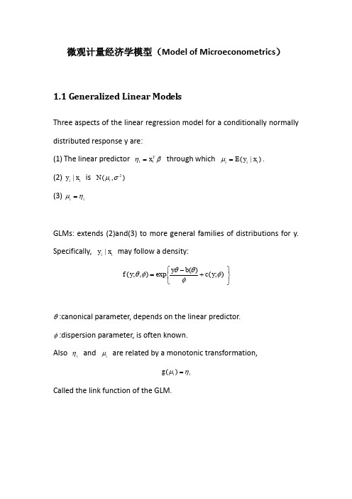
微观计量经济学模型（Model of Microeconometrics ）1.1 Generalized Linear Mod elsThree aspects of the linear regression model for a conditionally normally distributed response y are:(1) The linear predictor βηT i i x = through which )|(i i i x y E =μ. (2) i i x y | is ),(2σμi N (3) i i ημ=GLMs: extends (2)and(3) to more general families of distributions for y. Specifically, i i x y | may follow a density:⎭⎬⎫+⎩⎨⎧-=);()(exp ),;(φφθθφθy c b y y fθ:canonical parameter, depends on the linear predictor.φ:dispersion parameter, is often known.Also i η and i μ are related by a monotonic transformation,i i g ημ=)(Called the link function of the GLM.Selected GLM families and their canonical link1.2 Binary Depend ent VariablesModel:n i x F p x y E T i i i i ,......2,1),()|(===βIn the probit case: F equals the standard normal CDF In the logit case: F equals the logistic CDFExample:(1)DataConsidering female labor participation for a sample of 872 women from Switzerland.The dependent variable: participation The explain variables:income,age,education,youngkids,oldkids,foreignyesandage^2. R:library("AER")data("SwissLabor")summary(SwissLabor)participation income age educationno :471 Min. : 7.187 Min. :2.000 Min. : 1.000yes:401 1st Qu.:10.472 1st Qu.:3.200 1st Qu.: 8.000Median :10.643 Median :3.900 Median : 9.000Mean :10.686 Mean :3.996 Mean : 9.3073rd Qu.:10.887 3rd Qu.:4.800 3rd Qu.:12.000Max. :12.376 Max. :6.200 Max. :21.000 youngkids oldkids foreignMin. :0.0000 Min. :0.0000 no :6561st Qu.:0.0000 1st Qu.:0.0000 yes:216Median :0.0000 Median :1.0000Mean :0.3119 Mean :0.98283rd Qu.:0.0000 3rd Qu.:2.0000Max. :3.0000 Max. :6.0000(2) EstimationR:swiss_prob=glm(participation~.+I(age^2),data=SwissLabor,family=binomial(link="pro bit"))summary(swiss_prob)Call:glm(formula = participation ~ . + I(age^2), family = binomial(link = "probit"),data = SwissLabor)Deviance Residuals:Min 1Q Median 3Q Max-1.9191 -0.9695 -0.4792 1.0209 2.4803Coefficients:Estimate Std. Error z value Pr(>|z|)(Intercept) 3.74909 1.40695 2.665 0.00771 **income -0.66694 0.13196 -5.054 4.33e-07 ***age 2.07530 0.40544 5.119 3.08e-07 ***education 0.01920 0.01793 1.071 0.28428youngkids -0.71449 0.10039 -7.117 1.10e-12 ***oldkids -0.14698 0.05089 -2.888 0.00387 **foreignyes 0.71437 0.12133 5.888 3.92e-09 ***I(age^2) -0.29434 0.04995 -5.893 3.79e-09 ***---Signif. codes: 0 ‘***’ 0.001 ‘**’ 0.01 ‘*’ 0.05 ‘.’ 0.1 ‘ ’ 1 (Dispersion parameter for binomial family taken to be 1)Null deviance: 1203.2 on 871 degrees of freedomResidual deviance: 1017.2 on 864 degrees of freedomAIC: 1033.2Number of Fisher Scoring iterations: 4(3)VisualizationPlotting participation versus ageR:plot(participation~age,data=SwissLabor,ylevels=2:1)(4) Effectsj T i ijT i ij i i x x x x x y E ββφβ⋅=∂Φ∂=∂∂)()()|(Average marginal effects:The average of the sample marginal effects: j Ti n ix nββφ⋅∑)(1 R:fav=mean(dnorm(predict(swiss_prob,type="link"))) fav*coef(swiss_prob)(Intercept) income age education youngkids 1.241929965 -0.220931858 0.687466185 0.006358743 -0.236682273 oldkids foreignyes I(age^2) -0.048690170 0.236644422 -0.097504844The average marginal effects at the average regressor: R:av=colMeans(SwissLabor[,-c(1,7)])av=data.frame(rbind(swiss=av,foreign=av),foreign=factor(c("no","yes"))) av=predict(swiss_prob,newdata=av,type="link") av=dnorm(av)av["swiss"]*coef(swiss_prob)[-7] av["foreign"]*coef(swiss_prob)[-7]swiss:(Intercept) income age education youngkids 1.495137092 -0.265975880 0.827628145 0.007655177 -0.284937521 oldkids I(age^2) -0.058617218 -0.117384323Foreign:(Intercept) income age education youngkids 1.136517140 -0.202179551 0.629115268 0.005819024 -0.216593099 oldkids I(age^2) -0.044557434 -0.089228804(5) Goodness of fit and prediction Pseudo-R2:)()ˆ(12ββ-=R)ˆ(βas the log-likelihood for the fitted model, )(β )ˆ(β as the log-likelihood for the model containing only a constant term. R: swiss_prob0=update(swiss_prob,formula=.~1)1- as.vector(logLik(swiss_prob)/logLik(swiss_prob0))[1] 0.1546416Percent correctly predicted:R:table(true=SwissLabor$participation,pred=round(fitted(swiss_prob)))pred true 0 1 no 337 134 yes 146 25567.89% ROC curve:TPR(c):the number of women participating in the labor force that are classified as participating compared with the total number of womenparticipating.FPR(c):the number of women not participating in the labor force that are classified as participating compared with the total number of women not participating.R:l ibrary("ROCR")pred=prediction(fitted(swiss_prob),SwissLabor$participation)plot(performance(pred,"acc"))plot(performance(pred,"tpr","fpr"))abline(0,1,lty=2)Extensions: Multinomial responsesFor illustrating the most basic version of the multinomial logit model, a model with only individual-specific covariates,.data("BankWages")It contains, for employees of a US bank, an ordered factor job with levels "custodial", "admin"(for administration), and "manage" (for management), to be modeled as afunction of education (in years) and afactor minority indicating minority status. There also exists a factorgender, but since there are no women in the category "custodial", only a subset of the data corresponding to males is used for parametric modeling below.summary(BankWages)job education gender minoritycustodial: 27 Min. : 8.00 male :258 no :370admin :363 1st Qu.:12.00 female:216 yes:104manage : 84 Median :12.00Mean :13.493rd Qu.:15.00Max. :21.00summary(BankWages)edcat <- factor(BankWages$education)edcatlevels(edcat)[3:10] <- rep(c("14-15", "16-18", "19-21"),+ c(2, 3, 3))head(edcat)tab <- xtabs(~ edcat + job, data = BankWages)head(tab)prop.table(tab, 1)head(BankWages)library("nnet")bank_mn2 <- multinom(job ~ education + minority+gender,data=BankWages,trace = FALSE)summary(bank_mn2)1.3 Regression Mod els for Count DataWe begin with the standard model for count data, a Poisson regression.Poisson Regression Model:)ex p()|(βμT i i i i x x y E ==Canonical link: the log link Example:Trips to Lake Somerville,Texas,1980. based on a survey administered to 2,000 registered leisure boat owners in 23 counties in eastern Texas.The dependent variable is trips, and we want to regress it on all further variables: a (subjective) quality ranking of the facility (quality), a factor indicating whether the individual engaged in water-skiing at the lake (ski),household income (income), a factor indicating whether the individual paid a user’s fee at the lake (userfee), and three cost variables (costC, costS,costH) representing opportunity costs. (1)Datadata("RecreationDemand") summary(RecreationDemand)trips quality ski income userfee Min. : 0.000 Min. :0.000 no :417 Min. :1.000 no :646 1st Qu.: 0.000 1st Qu.:0.000 yes:242 1st Qu.:3.000 yes: 13Median : 0.000 Median :0.000 Median :3.000 Mean : 2.244 Mean :1.419 Mean :3.853 3rd Qu.: 2.000 3rd Qu.:3.000 3rd Qu.:5.000 Max. :88.000 Max. :5.000 Max. :9.000 costC costS costH Min. : 4.34 Min. : 4.767 Min. : 5.70 1st Qu.: 28.24 1st Qu.: 33.312 1st Qu.: 28.96 Median : 41.19 Median : 47.000 Median : 42.38 Mean : 55.42 Mean : 59.928 Mean : 55.993rd Qu.: 69.67 3rd Qu.: 72.573 3rd Qu.: 68.56Max. :493.77 Max. :491.547 Max. :491.05head(RecreationDemand)trips quality ski income userfee costC costS costH1 0 0 yes 4 no 67.59 68.620 76.8002 0 0 no 9 no 68.86 70.936 84.7803 0 0 yes 5 no 58.12 59.465 72.1104 0 0 no 2 no 15.79 13.750 23.6805 0 0 yes 3 no 24.02 34.033 34.5476 0 0 yes 5 no 129.46 137.377 137.850(2) Estimationrd_pois=glm(trips~.,data=RecreationDemand,family=poisson) coeftest(rd_pois)z test of coefficients:Estimate Std. Error z value Pr(>|z|) (Intercept) 0.2649934 0.0937222 2.8274 0.004692 ** quality 0.4717259 0.0170905 27.6016 < 2.2e-16 *** skiyes 0.4182137 0.0571902 7.3127 2.619e-13 *** income -0.1113232 0.0195884 -5.6831 1.323e-08 *** userfeeyes 0.8981653 0.0789851 11.3713 < 2.2e-16 *** costC -0.0034297 0.0031178 -1.1001 0.271309 costS -0.0425364 0.0016703 -25.4667 < 2.2e-16 *** costH 0.0361336 0.0027096 13.3353 < 2.2e-16 *** Signif. codes: 0 ‘***’ 0.001 ‘**’ 0.01 ‘*’ 0.05 ‘.’ 0.1 ‘R:logLik(rd_pois)the log-likelihood of the fitted model:'log Lik.' -1529.431 (df=8)rbind(obs = table(RecreationDemand$trips)[1:10], exp = round(+ sapply(0:9, function(x) sum(dpois(x, fitted(rd_pois))))))0 1 2 3 4 5 6 7 8 9obs 417 68 38 34 17 13 11 2 8 1exp 277 146 68 41 30 23 17 13 10 7table(true=RecreationDemand$trips,pred=round(fitted(rd_nb)))NOT WELL（3）Dealing with overdispersionPoisson distribution has the property that the variance equals the mean. In econometrics, Poisson regressions are often plagued by overdispersion. One way of testing for overdispersion is to consider the alternative hypothesis(Cameron and Trivedi 1990)Var(yi|xi) = μi + a*h(μi)where h is a positive function of μi.Overdispersion corresponds to a > 0 and underdispersion to a < 0. Common specifications of the transformation function h are h(μ) = μ2 or h(μ) = μ. The former corresponds to a negative binomial (NB) model (see below) with quadratic variance function (called NB2 by Cameron and Trivedi 1998), the latter to an NB model with linear variance function (called NB1 by Cameron and Trivedi 1998). In the statistical literature, the reparameterizationVar(yi|xi) = (1 + a) · μi = dispersion · μiof the NB1 model is often called a quasi-Poisson model with dispersion parameter.R: dispersiontest(rd_pois)Overdispersion testdata: rd_poisz = 2.4116, p-value = 0.007941alternative hypothesis: true dispersion is greater than 1sample estimates:dispersion6.5658R:dispersiontest(rd_pois, trafo = 2)Overdispersion testdata: rd_poisz = 2.9381, p-value = 0.001651alternative hypothesis: true alpha is greater than 0sample estimates:alpha1.316051Both suggest that the Poisson model for the trips data is not wellspecified.One possible remedy is to consider a more flexible distribution that does not impose equality of mean and variance.The most widely used distribution in this context is the negative binomial. It may be considered a mixture distribution arising from a Poisson distribution with random scale, the latter following a gamma distribution. Its probability mass function isR: library("MASS")rd_nb <- glm.nb(trips ~ ., data = RecreationDemand)coeftest(rd_nb)z test of coefficients:Estimate Std. Error z value Pr(>|z|)(Intercept) -1.1219363 0.2143029 -5.2353 1.647e-07 ***quality 0.7219990 0.0401165 17.9976 < 2.2e-16 ***skiyes 0.6121388 0.1503029 4.0727 4.647e-05 ***income -0.0260588 0.0424527 -0.6138 0.53933userfeeyes 0.6691676 0.3530211 1.8955 0.05802 .costC 0.0480087 0.0091848 5.2270 1.723e-07 ***costS -0.0926910 0.0066534 -13.9314 < 2.2e-16 ***costH 0.0388357 0.0077505 5.0107 5.423e-07 ***---Signif. codes: 0 ‘***’ 0.001 ‘**’ 0.01 ‘*’ 0.05 ‘.’ 0.1 ‘R:logLik(rd_nb)'log Lik.' -825.5576 (df=9)0 1 2 3 4 5 6 7 8 9obs 417 68 38 34 17 13 11 2 8 1exp 370 87 37 26 21 17 14 11 9 8(4)Zero-inflated Poisson and negative binomial modelsrbind(obs = table(RecreationDemand$trips)[1:10], exp = round(+ sapply(0:9, function(x) sum(dpois(x, fitted(rd_pois))))))0 1 2 3 4 5 6 7 8 9obs 417 68 38 34 17 13 11 2 8 1exp 277 146 68 41 30 23 17 13 1 0 7One such model is the zero-inflated Poisson (ZIP) model (Lambert 1992), which suggests a mixture specification with a Poisson count component and an additional point mass at zero. With I A(y) denoting the indicator function, the basic idea isf zeroinfl(y) = p i · I{0}(y) + (1 − p i) · f count(y; μi),we consider a regression of trips on all further variables for the count part (using a negative binomial distribution) and model the inflation part as a function of quality and income:library(pscl)rd_zinb = zeroinfl(trips ~ . | quality + income,data=RecreationDemand, dist="negbin")summary(rd_zinb )Call:zeroinfl(formula = trips ~ . | quality + income, data = RecreationDemand, dist = "negbin")Pearson residuals:Min 1Q Median 3Q Max-1.08885 -0.20037 -0.05696 -0.04509 40.01393Count model coefficients (negbin with log link):Estimate Std. Error z value Pr(>|z|)(Intercept) 1.096634 0.256679 4.272 1.93e-05 ***quality 0.168911 0.053032 3.185 0.001447 **skiyes 0.500694 0.134488 3.723 0.000197 ***income -0.069268 0.043800 -1.581 0.113775userfeeyes 0.542786 0.282801 1.919 0.054944 .costC 0.040445 0.014520 2.785 0.005345 **costS -0.066206 0.007745 -8.548 < 2e-16 ***costH 0.020596 0.010233 2.013 0.044146 *Log(theta) 0.190175 0.112989 1.683 0.092352 .Zero-inflation model coefficients (binomial with logit link):Estimate Std. Error z value Pr(>|z|)(Intercept) 5.7427 1.5561 3.691 0.000224 ***quality -8.3074 3.6816 -2.256 0.024041 *income -0.2585 0.2821 -0.916 0.359504---Signif. codes: 0 '***' 0.001 '**' 0.01 '*' 0.05 '.' 0.1 ' ' 1Theta = 1.2095Number of iterations in BFGS optimization: 26Log-likelihood: -722 on 12 DfR:rbind(obs =table(RecreationDemand$trips)[1:10],exp=round(colSums(predict(rd_zin b, type = "prob")[,1:10])))0 1 2 3 4 5 6 7 8 9obs 417 68 38 34 17 13 11 2 8 1exp 433 47 35 27 20 16 12 10 8 7。

18.Sequential Quadratic Programming

C H A P T E R18 Sequential Quadratic ProgrammingOne of the most effective methods for nonlinearly constrained optimization generates steps by solving quadratic subproblems.This sequential quadratic programming(SQP)approach can be used both in line search and trust-region frameworks,and is appropriate for small or large problems.Unlike linearly constrained Lagrangian methods(Chapter17),which are effective when most of the constraints are linear,SQP methods show their strength when solving problems with signiﬁcant nonlinearities in the constraints.All the methods considered in this chapter are active-set methods;a more descriptive title for this chapter would perhaps be“Active-Set Methods for Nonlinear Programming.”530C H A P T E R18.S E Q U E N T I A L Q U A D R A T I C P R O G R A M M I N GIn Chapter14we study interior-point methods for nonlinear programming,a competing approach for handling inequality-constrained problems.There are two types of active-set SQP methods.In the IQP approach,a general inequality-constrained quadratic program is solved at each iteration,with the twin goals of computing a step and generating an estimate of the optimal active set.EQP methods decouple these computations.Theyﬁrst compute an estimate of the optimal active set,then solve an equality-constrained quadratic program toﬁnd the step.In this chapter we study both IQP and EQP methods.Our development of SQP methods proceeds in two stages.First,we consider local methods that motivate the SQP approach and allow us to introduce the step computation techniques in a simple setting.Second,we consider practical line search and trust-region methods that achieve convergence from remote starting points.Throughout the chapter we give consideration to the algorithmic demands of solving large problems.18.1LOCAL SQP METHODWe begin by considering the equality-constrained problemmin f(x)(18.1a)subject to c(x) 0,(18.1b) where f:I R n→I R and c:I R n→I R m are smooth functions.The idea behind the SQP approach is to model(18.1)at the current iterate x k by a quadratic programming subproblem,then use the minimizer of this subproblem to deﬁne a new iterate x k+1.The challenge is to design the quadratic subproblem so that it yields a good step for the nonlinear optimization problem.Perhaps the simplest derivation of SQP methods,which we present now,views them as an application of Newton’s method to the KKT optimality conditions for(18.1).From(12.33),we know that the Lagrangian function for this problem is L(x,λ) f(x)−λT c(x).We use A(x)to denote the Jacobian matrix of the constraints,that is,A(x)T [∇c1(x),∇c2(x),...,∇c m(x)],(18.2) where c i(x)is the i th component of the vector c(x).Theﬁrst-order(KKT)conditions(12.34)of the equality-constrained problem(18.1)can be written as a system of n+mequations in the n+m unknowns x andλ:F(x,λ)∇f(x)−A(x)Tλc(x)0.(18.3)Any solution(x∗,λ∗)of the equality-constrained problem(18.1)for which A(x∗)has full18.1.L O C A L S Q P M E T H O D531 rank satisﬁes(18.3).One approach that suggests itself is to solve the nonlinear equations (18.3)by using Newton’s method,as described in Chapter11.The Jacobian of(18.3)with respect to x andλis given byF (x,λ)∇2xx L(x,λ)−A(x)TA(x)0.(18.4)The Newton step from the iterate(x k,λk)is thus given byx k+1λk+1x kλk+p kpλ,(18.5)where p k and pλsolve the Newton–KKT system∇2xx L k−A T kA k0p kpλ−∇f k+A T kλk−c k.(18.6)This Newton iteration is well deﬁned when the KKT matrix in(18.6)is nonsingular.We saw in Chapter16that this matrix is nonsingular if the following assumption holds at (x,λ) (x k,λk).Assumptions18.1.(a)The constraint Jacobian A(x)has full row rank;(b)The matrix∇2xx L(x,λ)is positive deﬁnite on the tangent space of the constraints,that is,d T∇2xx L(x,λ)d>0for all d 0such that A(x)d 0.Theﬁrst assumption is the linear independence constraint qualiﬁcation discussed in Chapter12(see Deﬁnition12.4),which we assume throughout this chapter.The second condition holds whenever(x,λ)is close to the optimum(x∗,λ∗)and the second-order suf-ﬁcient condition is satisﬁed at the solution(see Theorem12.6).The Newton iteration(18.5), (18.6)can be shown to be quadratically convergent under these assumptions(see Theo-rem18.4)and constitutes an excellent algorithm for solving equality-constrained problems, provided that the starting point is close enough to x∗.SQP FRAMEWORKThere is an alternative way to view the iteration(18.5),(18.6).Suppose that at the iterate(x k,λk)we model problem(18.1)using the quadratic programminpf k+∇f T k p+12p T∇2xx L k p(18.7a)subject to A k p+c k 0.(18.7b)532C H A P T E R18.S E Q U E N T I A L Q U A D R A T I C P R O G R A M M I N GIf Assumptions18.1hold,this problem has a unique solution(p k,l k)that satisﬁes∇2xx L k p k+∇f k−A T k l k 0,(18.8a)A k p k+c k 0.(18.8b)The vectors p k and l k can be identiﬁed with the solution of the Newton equations(18.6).If we subtract A T kλk from both sides of theﬁrst equation in(18.6),we obtain∇2xx L k−A T kA k0p kλk+1−∇f k−c k.(18.9)Hence,by nonsingularity of the coefﬁcient matrix,we have thatλk+1 l k and that p k solves (18.7)and(18.6).The new iterate(x k+1,λk+1)can therefore be deﬁned either as the solution of the quadratic program(18.7)or as the iterate generated by Newton’s method(18.5),(18.6) applied to the optimality conditions of the problem.Both viewpoints are useful.The Newton point of view facilitates the analysis,whereas the SQP framework enables us to derive practical algorithms and to extend the technique to the inequality-constrained case.We now state the SQP method in its simplest form.Algorithm18.1(Local SQP Algorithm for solving(18.1)).Choose an initial pair(x0,λ0);set k←0;repeat until a convergence test is satisﬁedEvaluate f k,∇f k,∇2xx L k,c k,and A k;Solve(18.7)to obtain p k and l k;Set x k+1←x k+p k andλk+1←l k;end(repeat)We note in passing that,in the objective(18.7a)of the quadratic program,we could replace the linear term∇f T k p by∇x L(x k,λk)T p,since the constraint(18.7b)makes the two choices equivalent.In this case,(18.7a)is a quadratic approximation of the Lagrangian function.This fact provides a motivation for our choice of the quadratic model(18.7):We ﬁrst replace the nonlinear program(18.1)by the problem of minimizing the Lagrangian subject to the equality constraints(18.1b),then make a quadratic approximation to the Lagrangian and a linear approximation to the constraints to obtain(18.7).INEQUALITY CONSTRAINTSThe SQP framework can be extended easily to the general nonlinear programming problemmin f(x)(18.10a)18.2.P R E V I E W O F P R A C T I C A L S Q P M E T H O D S533subject to c i(x) 0,i∈E,(18.10b)c i(x)≥0,i∈I.(18.10c)To model this problem we now linearize both the inequality and equality constraints to obtainf k+∇f T k p+12p T∇2xx L k p(18.11a)minpsubject to∇c i(x k)T p+c i(x k) 0,i∈E,(18.11b)∇c i(x k)T p+c i(x k)≥0,i∈I.(18.11c)We can use one of the algorithms for quadratic programming described in Chapter16to solve this problem.The new iterate is given by(x k+p k,λk+1)where p k andλk+1are the solution and the corresponding Lagrange multiplier of(18.11).A local SQP method for (18.10)is thus given by Algorithm18.1with the modiﬁcation that the step is computedfrom(18.11).In this IQP approach the set of active constraints A k at the solution of(18.11) constitutes our guess of the active set at the solution of the nonlinear program.If theSQP method is able to correctly identify this optimal active set(and not change its guessat a subsequent iteration)then it will act like a Newton method for equality-constrained optimization and will converge rapidly.The following result gives conditions under whichthis desirable behavior takes place.Recall that strict complementarity is said to hold at a solution pair(x∗,λ∗)if there is no index i∈I such thatλ∗i c i(x∗) 0.Theorem18.1(Robinson[267]).Suppose that x∗is a local solution of(18.10)at which the KKT conditions are satis-ﬁed for someλ∗.Suppose,too,that the linear independence constraint qualiﬁcation(LICQ)(Deﬁnition12.4),the strict complementarity condition(Deﬁnition12.5),and the second-ordersufﬁcient conditions(Theorem12.6)hold at(x∗,λ∗).Then if(x k,λk)is sufﬁciently close to(x∗,λ∗),there is a local solution of the subproblem(18.11)whose active set A k is the same asthe active set A(x∗)of the nonlinear program(18.10)at x∗.It is also remarkable that,far from the solution,the SQP approach is usually able to improvethe estimate of the active set and guide the iterates toward a solution;see Section18.7.18.2PREVIEW OF PRACTICAL SQP METHODSIQP AND EQPThere are two ways of designing SQP methods for solving the general nonlinear programming problem(18.10).Theﬁrst is the approach just described,which solves at534C H A P T E R18.S E Q U E N T I A L Q U A D R A T I C P R O G R A M M I N Gevery iteration the quadratic subprogram(18.11),taking the active set at the solution of this subproblem as a guess of the optimal active set.This approach is referred to as the IQP(inequality-constrained QP)approach;it has proved to be quite successful in practice.Its main drawback is the expense of solving the general quadratic program(18.11),which can be high when the problem is large.As the iterates of the SQP method converge to the solution,however,solving the quadratic subproblem becomes economical if we use information from the previous iteration to make a good guess of the optimal solution of the current subproblem.This warm-start strategy is described below.The second approach selects a subset of constraints at each iteration to be the so-called working set,and solves only equality-constrained subproblems of the form(18.7),where the constraints in the working sets are imposed as equalities and all other constraints are ignored.The working set is updated at every iteration by rules based on Lagrange multiplier estimates,or by solving an auxiliary subproblem.This EQP(equality-constrained QP) approach has the advantage that the equality-constrained quadratic subproblems are less expensive to solve than(18.11)in the large-scale case.An example of an EQP method is the sequential linear-quadratic programming (SLQP)method discussed in Section18.5.This approach constructs a linear program by omitting the quadratic term p T∇2xx L k p from(18.11a)and adding a trust-region constraint p ∞≤ k to the subproblem.The active set of the resulting linear programming sub-problem is taken to be the working set for the current iteration.The method thenﬁxes the constraints in the working set and solves an equality-constrained quadratic program(with the term p T∇2xx L k p reinserted)to obtain the SQP step.Another successful EQP method is the gradient projection method described in Section16.7in the context of bound con-strained quadratic programs.In this method,the working set is determined by minimizinga quadratic model along the path obtained by projecting the steepest descent direction ontothe feasible region.ENFORCING CONVERGENCETo be practical,an SQP method must be able to converge from remote starting points and on nonconvex problems.We now outline how the local SQP strategy can be adapted to meet these goals.We begin by drawing an analogy with unconstrained optimization.In its simplest form,the Newton iteration for minimizing a function f takes a step to the minimizer of the quadratic modelm k(p) f k+∇f T k p+12p T∇2f k p.This framework is useful near the solution,where the Hessian∇2f(x k)is normally positive deﬁnite and the quadratic model has a well deﬁned minimizer.When x k is not close to the solution,however,the model function m k may not be convex.Trust-region methods ensure that the new iterate is always well deﬁned and useful by restricting the candidate step p k18.3.A L G O R I T H M I C D E V E L O P M E N T535 to some neighborhood of the origin.Line search methods modify the Hessian in m k(p)to make it positive deﬁnite(possibly replacing it by a quasi-Newton approximation B k),to ensure that p k is a descent direction for the objective function f.Similar strategies are used to globalize SQP methods.If∇2xx L k is positive deﬁnite onthe tangent space of the active constraints,the quadratic subproblem(18.7)has a unique solution.When∇2xx L k does not have this property,line search methods either replace itby a positive deﬁnite approximation B k or modify∇2xx L k directly during the process of matrix factorization.In all these cases,the subproblem(18.7)becomes well deﬁned,but themodiﬁcations may introduce unwanted distortions in the model.Trust-region SQP methods add a constraint to the subproblem,limiting the step toa region within which the model(18.7)is considered reliable.These methods are able to handle indeﬁnite Hessians∇2xx L k.The inclusion of the trust region may,however,cause the subproblem to become infeasible,and the procedures for handling this situation complicatethe algorithms and increase their computational cost.Due to these tradeoffs,neither of thetwo SQP approaches—line search or trust-region—is currently regarded as clearly superiorto the other.The technique used to accept or reject steps also impacts the efﬁciency of SQP methods.In unconstrained optimization,the merit function is simply the objective f,and it remainsﬁxed throughout the minimization procedure.For constrained problems,we use devicessuch as a merit function or aﬁlter(see Section15.4).The parameters or entries used in these devices must be updated in a way that is compatible with the step produced by theSQP method.18.3ALGORITHMIC DEVELOPMENTIn this section we expand on the ideas of the previous section and describe various ingredients needed to produce practical SQP algorithms.We focus on techniques for ensuring that the subproblems are always feasible,on alternative choices for the Hessian of the quadratic model,and on step-acceptance mechanisms.HANDLING INCONSISTENT LINEARIZATIONSA possible difﬁculty with SQP methods is that the linearizations(18.11b),(18.11c)ofthe nonlinear constraints may give rise to an infeasible subproblem.Consider,for example,the case in which n 1and the constraints are x≤1and x2≥4.When we linearize these constraints at x k 1,we obtain the inequalities−p≥0and2p−3≥0,which are inconsistent.536C H A P T E R18.S E Q U E N T I A L Q U A D R A T I C P R O G R A M M I N GTo overcome this difﬁculty,we can reformulate the nonlinear program(18.10)as the 1penalty problemmin x,v,w,t f(x)+µi∈E(v i+w i)+µi∈It i(18.12a)subject to c i(x) v i−w i,i∈E,(18.12b)c i(x)≥−t i,i∈I,(18.12c)v,w,t≥0,(18.12d) for some positive choice of the penalty parameterµ.The quadratic subproblem(18.11) associated with(18.12)is always feasible.As discussed in Chapter17,if the nonlinear problem(18.10)has a solution x∗that satisﬁes certain regularity assumptions,and if the penalty parameterµis sufﬁciently large,then x∗(along with v∗i w∗i 0,i∈E and t∗i0,i∈I)is a solution of the penalty problem(18.12).If,on the other hand,there is no feasible solution to the nonlinear problem andµis large enough,then the penalty problem (18.12)usually determines a stationary point of the infeasibility measure.The choice ofµhas been discussed in Chapter17and is considered again in Section18.5.The SNOPT software package[127]uses the formulation(18.12),which is sometimes called the elastic mode,to deal with inconsistencies of the linearized constraints.Other procedures for relaxing the constraints are presented in Section18.5in the context of trust-region methods.FULL QUASI-NEWTON APPROXIMATIONSThe Hessian of the Lagrangian∇2xx L(x k,λk)is made up of second derivatives of the objective function and constraints.In some applications,this information is not easy to compute,so it is useful to consider replacing the Hessian∇2xx L(x k,λk)in(18.11a)by a quasi-Newton approximation.Since the BFGS and SR1formulae have proved to be successful in the context of unconstrained optimization,we can employ them here as well.The update for B k that results from the step from iterate k to iterate k+1makes use of the vectors s k and y k deﬁned as follows:s k x k+1−x k,y k ∇x L(x k+1,λk+1)−∇x L(x k,λk+1).(18.13) We compute the new approximation B k+1using the BFGS or SR1formulae given,respec-tively,by(6.19)and(6.24).We can view this process as the application of quasi-Newton updating to the case in which the objective function is given by the Lagrangian L(x,λ)(with λﬁxed).This viewpoint immediately reveals the strengths and weaknesses of this approach.If∇2xx L is positive deﬁnite in the region where the minimization takes place,then BFGS quasi-Newton approximations B k will reﬂect some of the curvature information of the problem,and the iteration will converge robustly and rapidly,just as in the unconstrained BFGS method.If,however,∇2xx L contains negative eigenvalues,then the BFGS approach18.3.A L G O R I T H M I C D E V E L O P M E N T537 of approximating it with a positive deﬁnite matrix may be problematic.BFGS updating requires that s k and y k satisfy the curvature condition s T k y k>0,which may not hold whens k and y k are deﬁned by(18.13),even when the iterates are close to the solution.To overcome this difﬁculty,we could skip the BFGS update if the conditions T k y k≥θs T k B k s k(18.14)is not satisﬁed,whereθis a positive parameter(10−2,say).This strategy may,on occasion,yield poor performance or even failure,so it cannot be regarded as adequate for general-purpose algorithms.A more effective modiﬁcation ensures that the update is always well deﬁned by modifying the deﬁnition of y k.Procedure18.2(Damped BFGS Updating).Given:symmetric and positive deﬁnite matrix B k;Deﬁne s k and y k as in(18.13)and setr k θk y k+(1−θk)B k s k,where the scalarθk is deﬁned asθk1if s T k y k≥0.2s T k B k s k,(0.8s T k B k s k)/(s T k B k s k−s T k y k)if s T k y k<0.2s T k B k s k;(18.15)Update B k as follows:B k+1 B k−B k s k s TkB ks TkB k s k+r k rTks Tkr k.(18.16)The formula(18.16)is simply the standard BFGS update formula,with y k replaced by r k.It guarantees that B k+1is positive deﬁnite,since it is easy to show that whenθk 1 we haves T k r k 0.2s T k B k s k>0.(18.17) To gain more insight into this strategy,note that the choiceθk 0gives B k+1 B k,while θk 1gives the(possibly indeﬁnite)matrix produced by the unmodiﬁed BFGS update.A valueθk∈(0,1)thus produces a matrix that interpolates the current approximation B k and the one produced by the unmodiﬁed BFGS formula.The choice ofθk ensures that the new approximation stays close enough to the current approximation B k to ensure positive deﬁniteness.538C H A P T E R18.S E Q U E N T I A L Q U A D R A T I C P R O G R A M M I N GDamped BFGS updating often works well but it,too,can behave poorly on difﬁcult problems.It still fails to address the underlying problem that the Lagrangian Hessian may not be positive deﬁnite.For this reason,SR1updating may be more appropriate,and is indeed a good choice for trust-region SQP methods.An SR1approximation to the Hessian of the Lagrangian is obtained by applying formula(6.24)with s k and y k deﬁned by(18.13), using the safeguards described in Chapter6.Line search methods cannot,however,accept indeﬁnite Hessian approximations and would therefore need to modify the SR1formula, possibly by adding a sufﬁciently large multiple of the identity matrix;see the discussion around(19.25).All quasi-Newton approximations B k discussed above are dense n×n matrices that can be expensive to store and manipulate in the large-scale case.Limited-memory updating is useful in this context and is often implemented in software packages.(See(19.29)for an implementation of limited-memory BFGS in a constrained optimization algorithm.) REDUCED-HESSIAN QUASI-NEWTON APPROXIMATIONSWhen we examine the KKT system(18.9)for the equality-constrained problem(18.1), we see that the part of the step p k in the range space of A T k is completely determined by the second block row A k p k −c k.The Lagrangian Hessian∇2xx L k affects only the part of p k in the orthogonal subspace,namely,the null space of A k.It is reasonable,therefore, to consider quasi-Newton methods thatﬁnd approximations to only that part of∇2xx L k that affects the component of p k in the null space of A k.In this section,we consider quasi-Newton methods based on these reduced-Hessian approximations.Our focus is on equality-constrained problems in this section,as existing SQP methods for the full problem(18.10)use reduced-Hessian approaches only after an equality-constrained subproblem hasbeen generated.To derive reduced-Hessian methods,we consider solution of the step equations(18.9) by means of the null space approach of Section16.2.In that section,we deﬁned matrices Y k and Z k whose columns span the range space of A T k and the null space of A k,respectively.By writingp k Y k p Y+Z k p Z,(18.18)and substituting into(18.9),we obtain the following system to be solved for pY and pZ:(A k Y k)pY −c k,(18.19a)Z T k∇2xx L k Z kpZ−Z T k∇2xx L k Y k p Y−Z T k∇f k.(18.19b)From theﬁrst block of equations in(18.9)we see that the Lagrange multipliersλk+1,which are sometimes called QP multipliers,can be obtained by solving(A k Y k)Tλk+1 Y T k(∇f k+∇2xx L k p k).(18.20)18.3.A L G O R I T H M I C D E V E L O P M E N T539We can avoid computation of the Hessian∇2xx L k by introducing several approx-imations in the null-space approach.First,we delete the term involving p k from theright-hand-side of(18.20),thereby decoupling the computations of p k andλk+1and elimi-nating the need for∇2xx L k in this term.This simpliﬁcation can be justiﬁed by observing thatp k converges to zero as we approach the solution,whereas∇f k normally does not.There-fore,the multipliers computed in this manner will be good estimates of the QP multipliers near the solution.More speciﬁcally,if we choose Y k A T k(which is a valid choice for Y k when A k has full row rank;see(15.16)),we obtainˆλk+1 (A k A T k)−1A k∇f k.(18.21) These are called the least-squares multipliers because they can also be derived by solving the problemmin λ ∇x L(x k,λ) 22∇f k−A T kλ22.(18.22)This observation shows that the least-squares multipliers are useful even when the current iterate is far from the solution,because they seek to satisfy theﬁrst-order optimality condition in(18.3)as closely as possible.Conceptually,the use of least-squares multipliers transforms the SQP method from a primal-dual iteration in x andλto a purely primal iteration in the x variable alone.Our second simpliﬁcation of the null-space approach is to remove the cross term Z Tk∇2xx L k Y k p Y in(18.19b),thereby yielding the simpler system(Z T k∇2xx L k Z k)p Z −Z T k∇f k.(18.23) This approach has the advantage that it needs to approximate only the matrix Z T k∇2xx L k Z k, not the(n−m)×m cross-term matrix Z T k∇2xx L k Y k,which is a relatively large matrixwhen m n−m.Dropping the cross term is justiﬁed when Z T k∇2xx L k Z k is replaced by aquasi-Newton approximation because the normal component pYusually converges to zerofaster than the tangential component pZ,thereby making(18.23)a good approximation of (18.19b).Having dispensed with the partial Hessian Z T k∇2xx L k Y k,we discuss how to approximate the remaining part Z T k∇2xx L k Z k.Suppose we have just taken a stepαk p k x k+1−x k αk Z k p Z+αk Y k p Y.By Taylor’s theorem,writing∇2xx L k+1 ∇2xx L(x k+1,λk+1),we have∇2xx L k+1αk p k≈∇x L(x k+αk p k,λk+1)−∇x L(x k,λk+1).By premultiplying by Z T k,we haveZ T k∇2xx L k+1Z kαk p Z(18.24)≈−Z T k∇2xx L k+1Y kαk p Y+Z T k[∇x L(x k+αk p k,λk+1)−∇x L(x k,λk+1)].540C H A P T E R18.S E Q U E N T I A L Q U A D R A T I C P R O G R A M M I N GIf we drop the cross term Z T k∇2xx L k+1Y kαk p Y(using the rationale discussed earlier),we see that the secant equation for M k can be deﬁned byM k+1s k y k,(18.25) where s k and y k are given bys k αk p Z,y k Z T k[∇x L(x k+αk p k,λk+1)−∇x L(x k,λk+1)].(18.26) We then apply the BFGS or SR1formulae,using these deﬁnitions for the correction vectors s k and y k,to deﬁne the new approximation M k+1.An advantage of this reduced-Hessian approach,compared to full-Hessian quasi-Newton approximations,is that the reduced Hessian is much more likely to be positive deﬁnite,even when the current iterate is some distance from the solution.When using the BFGS formula,the safeguarding mechanism discussed above will be required less often in line search implementations.MERIT FUNCTIONSSQP methods often use a merit function to decide whether a trial step should be accepted.In line search methods,the merit function controls the size of the step;in trust-region methods it determines whether the step is accepted or rejected and whether the trust-region radius should be adjusted.A variety of merit functions have been used in SQP methods,including nonsmooth penalty functions and augmented Lagrangians.We limit our discussion to exact,nonsmooth merit functions typiﬁed by the 1merit function discussed in Chapters15and17.For the purpose of step computation and evaluation of a merit function,inequality constraints c(x)≥0are often converted to the form¯c(x,s) c(x)−s 0,where s≥0is a vector of slacks.(The condition s≥0is typically not monitored by the merit function.)Therefore,in the discussion that follows we assume that all constraints are in the form of equalities,and we focus our attention on problem(18.1).The 1merit function for(18.1)takes the formφ1(x;µ) f(x)+µ c(x) 1.(18.27) In a line search method,a stepαk p k will be accepted if the following sufﬁcient decrease condition holds:φ1(x k+αk p k;µk)≤φ1(x k,µk)+ηαk D(φ1(x k;µ);p k),η∈(0,1),(18.28)18.3.A L G O R I T H M I C D E V E L O P M E N T541 where D(φ1(x k;µ);p k)denotes the directional derivative ofφ1in the direction p k.This requirement is analogous to the Armijo condition(3.4)for unconstrained optimization provided that p k is a descent direction,that is,D(φ1(x k;µ);p k)<0.This descent condition holds if the penalty parameterµis chosen sufﬁciently large,as we show in the following result. Theorem18.2.Let p k andλk+1be generated by the SQP iteration(18.9).Then the directional derivativeofφ1in the direction p k satisﬁesD(φ1(x k;µ);p k) ∇f T k p k−µ c k 1.(18.29) Moreover,we have thatD(φ1(x k;µ);p k)≤−p T k∇2xx L k p k−(µ− λk+1 ∞) c k 1.(18.30)P ROOF.By applying Taylor’s theorem(see(2.5))to f and c i,i 1,2,...,m,we obtain φ1(x k+αp;µ)−φ1(x k;µ) f(x k+αp)−f k+µ c(x k+αp) 1−µ c k 1≤α∇f T k p+γα2 p 2+µ c k+αA k p 1−µ c k 1,where the positive constantγbounds the second-derivative terms in f and c.If p p k is given by(18.9),we have that A k p k −c k,so forα≤1we have thatφ1(x k+αp k;µ)−φ1(x k;µ)≤α[∇f T k p k−µ c k 1]+α2γ p k 2.By arguing similarly,we also obtain the following lower bound:φ1(x k+αp k;µ)−φ1(x k;µ)≥α[∇f T k p k−µ c k 1]−α2γ p k 2.Taking limits,we conclude that the directional derivative ofφ1in the direction p k is given byD(φ1(x k;µ);p k) ∇f T k p k−µ c k 1,(18.31) which proves(18.29).The fact that p k satisﬁes theﬁrst equation in(18.9)implies thatD(φ1(x k;µ);p k) −p T k∇2xx L k p k+p T k A T kλk+1−µ c k 1.From the second equation in(18.9),we can replace the term p T k A T kλk+1in this expression by−c T kλk+1.By making this substitution in the expression above and invoking the inequality−c T kλk+1≤ c k 1 λk+1 ∞,we obtain(18.30).。

1、下载文档前请自行甄别文档内容的完整性，平台不提供额外的编辑、内容补充、找答案等附加服务。
2、"仅部分预览"的文档,不可在线预览部分如存在完整性等问题,可反馈申请退款(可完整预览的文档不适用该条件!)。
3、如文档侵犯您的权益，请联系客服反馈,我们会尽快为您处理(人工客服工作时间：9:00-18:30)。

A micro-constraint model of Optimality Theory:Do infantslearn universal constraints?Robert D.KyleVNMaster of ScienceCognitive Science and Natural Language ProcessingSchool of InformaticsUniversity of Edinburgh2005AbstractDoes Optimality Theory offer a basis for a neurologically plausible model of language?This paper examines the case for Optimality Theory as a plausible model of language,and suggests modiﬁcations to the theory that would improve the biological plausibility,learnability,and co-herence of the model.The micro-constraint model which emerges from these modiﬁcations, suggests that language,and linguistic universal behaviour is learned by settling upon an arbitrary set micro-constraints,rather than acquiring or ranking innate constraints as speciﬁed by Opti-mality Theory.The validity of this micro-constraint model is tested using a Simple Recurrent Network model of speech syllabiﬁcation,and some support is found for the claim that arbitrary micro-constraints might reproduce universal constraints.However,we suggest that further work, with fewer assumptions about the nature of the speech stream is needed in order to improve the conclusiveness of the result.iAcknowledgementsI would like to thank my supervisor,Mark Steedman,for his helpful guidance and advice throughout the project.I would also like to thank Mits Ota,for his considerable help on aspects of Optimality Theory, and insightful comments on the experiment.Last but not least,thanks to Lexi and Sara,whose presence in the MSc lab helped while away the three months spent on this project.Their lunchtime banter and considerable knowledge of esoteric perl and latex syntax was instrumental to the success of this project.iiDeclarationI declare that this thesis was composed by myself,that the work contained herein is my own except where explicitly stated otherwise in the text,and that this work has not been submitted for any other degree or professional qualiﬁcation except as speciﬁed.(Robert D.Kyle)iiiTable of Contents1Introduction11.1Overview (1)1.2The structure of the thesis (2)2Background42.1Optimality Theory:a neurologically plausible model of language? (4)2.1.1Why Optimality Theory is deeply connected to connectionism (4)2.1.2Why Optimality Theory has nothing to do with connectionism (8)2.1.3Is strict domination an empirical fact? (11)2.1.4Are universal constraints and strict domination necessary? (11)2.2Universal constraints:more trouble than they are worth? (12)2.2.1The learnability of universal constraints (12)2.2.2The neurological plausibility of universal constraints (13)2.2.3The biological plausibility of universal constraints (14)2.3Micro-constraints:a solution to OT’s problems? (14)2.3.1Optimality Theory at the microscopic level (14)2.3.2How learned micro-constraints might imitate universal macro-constraints152.3.3How micro-constraints offer a simpliﬁed architecture (17)2.3.4Stochastic interpretations of Optimality Theory (17)2.4Recapitulation:The features of a micro-constraint model of Optimality Theory.183Design193.1The theoretical claim (19)3.2How the claim can be tested (19)iv3.3The syllabiﬁcation problem (21)3.4Experimental hypothesis (22)4Method234.1Assembly of the corpora (23)4.2Experimental method (25)5Results275.1Assessing acquisition of phonology (27)5.2Assessing syllabiﬁcation performance (27)5.2.1Test of the experimental hypothesis (30)6Discussion346.1Support for the hypothesis (34)6.1.1How should syllabiﬁcation be measured? (34)6.1.2The difﬁculty of”doing Optimality Theory in a straitjacket” (35)6.1.3A preference for words with no coda (36)6.2Methodological Issues (36)6.2.1The corpus (36)6.2.2The model (38)6.3Interpretation of the results (39)6.4What is the use of a micro-constraint model of Optimality Theory? (40)7Future Work427.1Unsupervised learning of phonology (42)8Conclusion44 Bibliography45A Phonological key48B Phonetic feature table50vChapter1Introduction1.1OverviewThis thesis is focused upon constraint-based approaches to language,and in particular,the neu-rological plausibility of existing linguistic theories,such as Optimality Theory.Constraint based approaches to language offer an interesting basis for exploration of the plausibility of linguis-tic theories,because they describe language using a framework which has its roots in neural network research.This thesis examines the case for Optimality Theory as a neurologically plau-sible model of language,and suggests that the plausibility of the model would be improved if claims of universal constraints and strict domination were dropped.We argue that the intro-duction of universal constraints,which in turn motivates strict domination,serves to make the theory less biologically plausible,and reduces learnability of languages in the resulting model. We propose,that Optimality Theory is better conceived at the microscopic level,and that a more coherent model of language emerges if we consider the overall behaviour of Optimality Theory constraints to be as a result of the interaction of microscopic constraints at the neural level.This micro-constraint model of Optimality Theory implies that the universal constraints observed at a higher level,are in fact learned,and can be produced by any combination of micro-constraints which provide functionally equivalent behaviour to the high-level macro-constraints.This micro-constraint model of Optimality Theory is put to the test by examining whether a model that has learned to perform at a particular linguistic task by modifying internal micro-constraints,actu-ally displays behaviour,which at a higher-level of analysis can be attributed to a knowledge of the universal macro-constraints.We describe such an experiment by training a Simple Recur-1rent Network to predict syllable boundaries,and examining whether its syllabiﬁcation behaviour implies implicit knowledge of Optimality Theory constraints relevant to syllabiﬁcation.The test of the experimental hypothesis at the syllable level returns an inconclusive result, do to the considerable simplifying assumptions that were made in constructing the model and corpus.However,a test of the experimental hypothesis at the word level supports the hypothesis, and implies that the model has indeed learned a set of micro-constraints that display universal macro-constraint behaviour.We conclude by suggesting ways in which a more conclusive result might be reached,and discuss future work which could be used to further investigate this model.1.2The structure of the thesisChapter2In this chapter we introduce Optimality Theory in its historical context,and examine the properties which may or may not offer the model some neurological plausibility.We suggest areas in which the model might be modiﬁed to improve its coherence,and assess the consequences of making these modiﬁcations.Chapter3In the Design chapter we state an experimental claim motivated by the evidence described in the previous chapter.This claim is used to design an experimental test using a model of speech syllabiﬁcation.The chapter concludes with an experimental hypothesis.Chapter4Chapter4describes experimental method,including the generation of the training data from a corpus of Child-directed speech,and the construction of the syllabiﬁcation model.Chapter5In chapter5we report the model’s performance on predicting the next phoneme ina speech stream,and evaluate the model’s syllabiﬁcation preference.The model’s perfor-mance on syllabiﬁcation at word and syllable levels is used to examine the experimental hypothesisChapter6In this chapter we analyse the results reported in the previous chapter,and discuss on what grounds the experimental hypothesis is supported.We point out shortcomings of the model both theoretical and methodological,and we suggest ways in which the corpus and model could be modiﬁed to provide more conclusive evidence.We also discuss the relevance of the experimental claim,and the utility of the model proposed in chapter2.Chapter7This chapter includes a discussion of future work which might provide a more con-clusive test of the model.In particular we examine the possibility of constructing unsuper-vised models of phonological acquisition using recurrent self-organising maps.We also discuss previous language models which have made use of these architectures.Chapter8Conclusion.Chapter2Background2.1Optimality Theory:a neurologically plausible model oflanguage?This thesis is concerned with the neurological plausibility of existing linguistic theories,and for that reason we have chosen to examine the properties of Optimality Theory.Optimality Theory was chosen for study because it offers an interesting perspective on the issue for two reasons:1.It has been successful in phonology where generative models have failed.2.It describes language using mechanisms that are compatible with the way in which thebrain works.As such,it provides a interesting avenue to explore neurologically plausible descriptions of lan-guage.In this chapter we will examine the case for Optimality Theory as a neurologically plau-sible model of language,and we will suggest modiﬁcations that would improve its learnability and biological plausibility.2.1.1Why Optimality Theory is deeply connected to connectionism1Although Optimality Theory wasﬁrst introduced in1993(Prince and Smolensky,1993)and is a relatively new model,the roots of the theory stretch back further,to Harmonic Grammar(Smolensky et al.,1992),a model of language that was inspired by computational mechanisms developed in neural network research.Rather than describe language as a generative formal system which deﬁnes the legal forms of a language,Optimality Theory and Harmonic Grammar both describe language as a set of constraints which interact to determine the optimal parse.In Harmonic Grammar,the optimal parse is the one for which the numerical rankings of the violated constraints sum to the lowest value.Optimality Theory and Harmonic Grammar both claim that the constraints that are needed to adequately describe the empirical data,are a set of constraints that are universal to all languages. In these models,the differences between languages arise as a result of speakers’ranking the con-straints in subtly different ways.The difference between the Optimality Theory and Harmonic Grammar is that Harmonic Grammar originally claimed that constraints could potentially take any ranking value,whilst Optimality Theory has since proposed that the universal constraints are ranked ordinally,and obey a principle known as strict domination.The optimal version of any parse in Harmonic Grammar or Optimality Theory is often calculated using a constraint tableau, such as the one shown inﬁgure2.1.Candidate words or utterances are written on one side of the tableau,and the constraints which they violate are marked in the appropriate columns.The two theories differ in the way that the constraints interact to determine which candidate is optimal.The system of interacting constraints described by Harmonic Grammar was directly inspired by the behaviour of weights in Neural Networks,which act as constraints upon the activation of neurons.Prior to introducing Harmonic Grammar,Smolensky developed Harmony Theory (Smolensky,1986),a model of the activation dynamics that occur in certain classes of neural networks.The analysis introduced by Harmony Theory implied that networks with an architec-ture comparable to biological networks2were extremely well designed to rapidly solve constraint satisfaction problems.Perhaps it was reasoned,that if language had developed by exploiting the computational abilities of the brain,then the mechanisms of constraint satisfaction might provide a useful framework in which to understand language.The extent to which Harmonic Grammar and Optimality Theory are inspired by connectionist research can be seen in the use of the term Harmony to describe the degree of optimality of each parse.Harmony,from Harmony Theory,is a quantitative value which deﬁnes the degree to which the constraints(competing weights)in a neural network are satisﬁed at any point inFigure2.1:A constraint tableau in Optimality Theory.The table shows a list of candidates on the left hand side,and relevant constraints along the top.Asterisks indicate a violation of the con-straint,with an exclamation indicating the fatal violation.PARSE is greyed out where the violation of a higher ranked constraint has ruled out this candidate.The optimal candidate is the one which least violates the constraints in order of their ranking.Figure2.2:The way in which Optimality Theory and Harmonic Grammar deﬁne language can be viewed as a set of constraints which deﬁne the space of permissible utterances in a particular language.In this view,constraints are circles demarcating the space of utterances that each constraint allows.Each circle has a radius r n which reﬂects the ranking of the constraint.An utterance within a particular language may fall anywhere within the total space,and its Harmony can be calculated by summing the radius’of the circles the utterance falls within(the constraints which permit this utterance).In this example,the Harmony of utterance a r1,b r1r2, c r1r2r3,and d r3time.Harmony in a neural network increases monotonically towards attractor states,which once reached,are stable enough to drive activation in other areas of the network,much in the same way as stable perception of a particular concept can lead to a linguistic,motor,or other cognitive response.These harmony dynamics are present in all bi-directionally connected networks,and so given their close links with biological networks,these mechanisms provide a plausible basis from which to build a model of language.2.1.2Why Optimality Theory has nothing to do with connectionism3There are two distinct arguments as to why Optimality Theory is incompatible with connectionist descriptions of language.1.Purely connectionist approaches to language are incompatible with the goals of the In-tegrated connectionist/symbolic(ICS)paradigm in Cognitive Science(Smolensky et al., 1992).As a result,proponents of ICS have attempted to distance themselves from connec-tionist interpretations of Optimality Theory.2.Strict domination of constraints cannot plausibly occur at the neural level.2.1.2.1Optimality Theory and the Integrated Connectionist-Symbolic paradigmIn order to understand the unusual position taken by Optimality Theory,the argument must be viewed in the context of the Integrated connectionist/symbolic(ICS)paradigm.The ICS paradigm stems from the belief that in order to explain fully the nature of cognition,a theory must provide a description at both the symbolic and sub-symbolic level.Explanations which favour one level,and eliminate the other are unacceptable to the proponents of ICS.Since the introduction of Optimality Theory,this stance has forced the model to develop its symbolic credentials in order to improve its standing as an integrative theory.At the present time,the overwhelming majority of work within Optimality Theory has concentrated on its validity as a symbolic model of language,and little attention has been paid to its decreasing plausibility at the neural level.In fact,modiﬁcations to the theory motivated by symbolic considerations have rendered Optimality Theory incompatible with simple connectionist models,let alone the complex networks that occur in the brain.ICS’s stance as to what a valid model of cognition must consist of means that connectionist interpretations of Optimality Theory are typically viewed as either implementationist or elimina-tivist:either the model merely implements symbolic linguistic processing,and therefore by itself is an incomplete model,or it eliminates the need for a symbolic description,and is therefore not a valid model of cognition.Catch22!”All of the prototypical objectives in eliminativist research are completely anti-thetical to Optimality Theory.And as for the implementationalist approach,ratherthan arguing for the contribution of Optimality Theory based on issues of connec-tionist implementation,we have not even entertained the question.”(Prince andSmolensky,1993)This kind of logic has discouraged researchers working outside of the ICS paradigm from contributing to theﬁeld-any attempts to suggest sub-symbolic modiﬁcations to the theory are likely to be ruled out a priori,as an attempt to eliminate the symbolic level of description.2.1.2.2Differences between Optimality Theory and Harmonic GrammarOriginally,Harmonic Grammar was introduced as a model of language alongside the ICS paradigm, but developments in Harmonic Grammar eventually led to the introduction of Optimality The-ory,a special case of Harmonic Grammar in which constraints are ranked ordinally,rather than numerically4.”Phonological applications of Harmonic Grammar led Alan Prince and myself to a remarkable discovery:in a broad set of cases,at least,the relative strengthsof constraints need not be speciﬁed numerically.For if the numerically weightedconstraints needed in these cases are ranked from strongest to weakest,it turns outthat each constraint is stronger than all the weaker constraints combined.That is,thenumerical strengths are so arranged that each constraint can never be overruled byweaker constraints,no matter how many.”(Smolensky,1995)While the introduction of strict domination might have been empirically motivated,it quite clearly damages Optimality Theory’s validity as a sub-symbolic model.For reasons we shall discuss later,strict domination of constraints is not something which can plausibly occur in biological networks of neurons.Figure2.3:Now we can see more clearly how Optimality Theory differs from Harmonic Grammar usingﬁgure2.2.Optimality Theory can be seen as a special case of Harmonic Grammar where the rankings of the constraints(the radius’of the circles)are distributed along an exponential scale.The result is that no combination of lower ranked constraints can produce a Harmony value greater than a highly ranked constraint.For example,the ranking of permissible constraints is deﬁned so that r3r2r2r1,and therefore d b aSo does strict domination conclusively count out Optimality Theory as a neurally plausible model?Possibly not.The fact that connectionism is antithetical to ICS should not discourage re-searchers from pursuing the consequences of a connectionist interpretation of the theory.Those who do not accept the necessity of integrated connectionist/symbolic explanations in Cognitive Science need not be concerned that a neural interpretation of Optimality Theory might not grant symbolic structures the same ontological relevance as the standard model.Also,the argument that strict domination renders Optimality Theory incompatible with connectionist models of lan-guage is far from sound.The argument depends upon the following assumptions1.That strict domination is an empirical fact2.That the constraints in Optimality Theory are universalIn the next section we will examine the evidence for these two assumptions.2.1.3Is strict domination an empirical fact?Although the introduction of strict domination was motivated by observations in phonology,there are now well established cases where strict domination is broken(Joanisse,2000).One example of this is local conjunction(Ito and Mester,1998),whereby a violation of a conjunction of lower ranked constraints is enough to overrule a more highly ranked constraint.Mechanisms such as Sympathy Theory(McCarthy,1999)have been suggested as modiﬁcations to Optimality Theory that would allow for strict domination to be broken occasionally.But these modiﬁcations should ring alarm bells when claims are made of empirical support for strict domination.2.1.4Are universal constraints and strict domination necessary?Despite the example of local conjunction,there are actually relatively few case of strict domina-tion being broken.Perhaps the question we should be asking is”Why are there so few examples of strict domination being broken?”The answer to this question might lie in the considerable controversy over what can be con-sidered a constraint in Optimality Theory(Eisner,1999).It is not clear on which basis the Universal constraint set(CON)was discovered or chosen-were constraints that might break strict domination discarded in the initial deﬁnition of CON?Obviously,if we are free to choose any constraints,then it should always be possible to pick a set of constraints which will display strictdomination.The arbitrary nature of CON has also been questioned by Ellison,who has suggested that the Universal constraint is better supported as a convention,rather than fact(Ellison,2000). One of the major criticisms of Optimality Theory is aimed at the extremeﬂexibility of its choice of constraints.There are no obvious reasons why absurd constraints such as PALINDROMIC5 (Eisner,1999)or FRENCH6should be any less valid than those in the Universal constraint set.The existence and signiﬁcance of linguistic universals is a controversial topic,but there is enough evidence to suggest that many of these linguistic universals can be regarded as epiphe-nomenal features of a shared biological,social,and linguistic heritage.Or even as universal solutions to the problem of efﬁcient communication in a noisy environment.If there were a set of linguistic universals,it is not clear why they should be described at the level of folk-psychological linguistic units,as they are in Optimality Theory.If linguistic univer-sals have emerged as a by-product of agents with a shared cognitive apparatus communicating in a noisy environment,there is no obvious reason why these constraints should only be deﬁned in terms of arbitrary linguistic units,rather than a more messy set of constraints which are related to the biological apparatus of speech and cognition.To conclude,Optimality Theory’s claim to a language-speciﬁc universal constraint set can be called into question,without having to deny the existence of universal linguistic behaviour.We will now turn our attention to Optimality Theory’s claim of a universal constraint set,and the effect this has on the learnability and plausibility of the model.2.2Universal constraints:more trouble than they are worth?If the legitimacy of the universal constraint set is still an open question,perhaps we should re-examine this assumption,and ask whether or not universal constraints and strict domination are a worthy exchange for the models neurological plausibility.2.2.1The learnability of universal constraintsOne way in which we can observe the effect of universal constraints is the learnability of language within the Optimality Theory framework.Figure2.4:The architecture of Optimality Theory.A mechanism GEN generates candidate sets based upon the input,and these sets are evaluated toﬁnd the most optimal parse,which is passed on to the output.By requiring infants toﬁnd a particular ranking of a speciﬁc set of universal constraints, theorists have introduced a massive learning problem.Even if the universal constraints were somehow innate,there are a factorial number of possible rankings.Despite this apparent learning problem,Smolensky and Tesar have proposed the Constraint Demotion algorithm,which given CON,can rank the constraints,and learn certain classes of grammars within N(N-1)informative examples,where N is the number of constraints(Tesar and Smolensky,2000).However,this work assumes that the universal constraint set is innate,and is also depen-dent upon an architectural model which has no biological plausibility(something which ICS proponents believe is not a pressing concern).The constraint demotion algorithm suggested by Smolensky and Tesar also experiences problems with empirical data,as it cannot account for the way in which stages of language acquisition overlap,and the learners tendency towards regres-sion.(Curtin,2000).2.2.2The neurological plausibility of universal constraintsIf we accept the claim of an innate universal constraint set,and therefore the existence of strict domination,it is very difﬁcult to see how Optimality Theory might relate to neural processing.At the neural level,’innately speciﬁed’weights between neurons would need to line up along an exponential scale,so that no combination of lower ranked constraints could overcome a higher ranked constraint(Smolensky et al.,ress).Although this is highly implausible at a low level,itis not infeasible that moreﬂexible low-level constraints might display strict domination-like behaviour at a macroscopic level-we will explore this possibility later.2.2.3The biological plausibility of universal constraintsFinally,and most signiﬁcantly,given the difﬁculty of learning speciﬁc universal constraints, the suggestion that the problem may be solved by claiming that children are born with these constraints is not a biologically plausible hypothesis.There is no biological or neurological evidence that could support the claim that a linguistic-speciﬁc set of constraints are innate,in fact many developmental neuroscientists reject the very notion of innate behaviour(Elman et al., 1996).As discussed in section2.1.4,there are plenty of ways in which linguistic universals might emerge,without having to rely upon a speciﬁc set of linguistic constraints.Given the long list of theoretical problems introduced by claiming universal constraints,we suggest that the theory would be better off dropping the requirement of a universal constraint set,and allowing any set of constraints that provide functionally equivalent behaviour to that observed by linguists.2.3Micro-constraints:a solution to OT’s problems?2.3.1Optimality Theory at the microscopic levelAs we have discussed in section2.1.1,Optimality Theory borrows much of its computational mechanisms from Harmony Theory,a model of the activation dynamics that occur in bi-directionally connected neural networks.Harmony measures the extent to which the constraints(or weights) learned by the network are satisﬁed by a particular input.Harmony is deﬁned by the following equation2.5.1HFigure2.5:At t0,Unit C has an activation of1,and units A and B an activation of0.The competing constraints deﬁned by the weights interact toﬁnd the most Harmonious state as t∞. Note how quickly the Harmony reaches its maximum value-these networks are almost optimally designed for this task.units.Harmony in these networks increases monotonically to a state1that is stable in the absenceof further input to the network.These stable states are hypothesised to drive activation in other areas,so can be viewed as representing the optimally Harmonic state,or at a much higher level,as representing an interpretation of the input utterance,given the constraints learned by the network.The process of parallel constraint satisfaction,and the monotonic increase in harmony is showninﬁgure2.5.These bi-directionally connected networks display behaviour which makes them almost opti-mally adapted to the problem of dealing with linguistic input-their ability to resolve ambiguous input in parallel is an inherent feature of their architecture.2.3.2How learned micro-constraints might imitate universal macro-constraintsWe’ve seen how activation dynamics at the neural level provide the basis for the Optimality Theory framework,and so the question that we must now address is whether the macroscopic behaviour observed in Optimality Theory needs strict domination and a universal constraint setin order to reproduce the behaviour observed by linguists.。