高级微观经济学 (黄有光) AdMicro-L1-MathTools
高级微观经济学AdvancedMicroeconomics
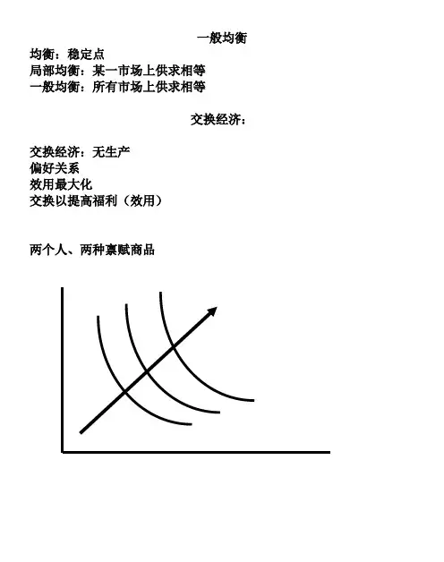
一般均衡均衡:稳定点局部均衡:某一市场上供求相等一般均衡:所有市场上供求相等交换经济:交换经济:无生产偏好关系效用最大化交换以提高福利(效用)两个人、两种禀赋商品Edgeworth 图 禀赋点为e假设自主交换能够实现帕累托改进,达到更优的配置点x对消费者1,其所偏好e 的区域为红色区域,最终的配置点必须在这一区域内,否那么,他拒绝交换或抵制这一配置。
对消费者2,其所偏好e 的区域为蓝色区域,最终的配置点必须在这一区域内,否那么,他拒绝交换或抵制这一配置。
因此,最终的配置点必须在重叠的区域中——凸透镜区域内和边上。
在这一区域里,双方或至少一方的福利能够提高。
11ee设交换后形成的配置点'x 在凸透镜内部,双方福利都得到改善,同时各有一条无差异曲线交于此点。
双方进一步通过交换改善彼此福利。
对消费者1,其所偏好'x 的区域为红色区域,最终的配置点必须在这一区域内,否那么,他拒绝交换或抵制这一配置。
对消费者2,其所偏好'x 的区域为蓝色区域,最终的配置点必须在这一区域内,否那么,他拒绝交换或抵制这一配置。
因此,最终的配置点必须在重叠的区域中——凸透镜区域内和边上。
在这一区域里,双方或至少一方的福利能够提高。
11ee'x交换过程持续下去,凸透镜越来越小,最终变为一个点:两条无差异曲线的切点:x 。
此时,双方进一步交换会使某一方福利下降。
所以,双方的交换一旦达到了切点位置,就不会有交换发生。
实现了帕累托最优。
在凸透镜内部和边上,这样的点有无数多个,最终的配置究竟是哪一个点,我们并不知道,或者说,我们不知道决定最终的帕累托效率点的位置的因素是什么。
结论只是:帕累托效率点位于凸透镜边上或内部的某个切点位置上。
11eexEdgeworth图中,所有的无差异曲线的切点的连线构成契约线,帕累托效率点是凸透镜与契约线交集中的点。
2 11eex当禀赋点落在契约线上时,即为帕累托效率点,无交换发生。
高级微观经济学

高级微观经济学
高级微观经济学(Advanced Microeconomics)是经济学中的一个分支,它深入研究个体经济主体和市场之间的相互关系。
与基础微观经济学相比,高级微观经济学更加理论性和复杂,涉及更深层次的经济学原理和模型。
高级微观经济学的研究内容包括:
1. 个体消费者和生产者的行为:研究消费者如何做出消费决策,生产者如何决定生产规模和价格。
2. 市场结构和竞争:研究市场的竞争程度和不完全竞争条件下的市场行为,如寡头垄断、垄断和寡头竞争。
3. 市场失灵:研究市场存在的各种制度和机制不完善导致的市场失灵现象,如外部性、公共物品和信息不对称等问题。
4. 游戏论和博弈论:研究个体之间的战略互动和决策过程,探讨不同策略下可能的结果。
5. 经济激励和合同理论:研究如何通过激励机制和合同设
计来引导经济主体的行为,如契约理论和机制设计等。
6. 不完全信息和不确定性:研究在信息有限和不确定性条
件下个体的决策行为和市场运行情况。
高级微观经济学的研究方法强调理论建模和分析,常常使
用数学和形式化的方法来描述经济行为和市场机制。
它是
经济学家、政策制定者和企业家等经济管理者理解经济现
象和制定决策的重要工具。
《高级微观经济学Advanced Microeconomics》课件PPT-l
2.Properties of PS.
• Additive (free entrance) :
y Y,and y Y, then y y Y • Convexity: y Y,and y Y, then y (1 )y Y, here [0,1]
See the fig.
• Proposition1: if Y is convex, so is V(q). • Proposition2: if V(q) is convex, f(x) is quasiconcave.
lecture 1 for Chu Kechen Honors College
y Y, ay Y, a 0
lecture 1 for Chu Kechen Honors College
4.Returns to scale
• Proposition 3: Y is constant returns to
scale if Y is both “additive” and “convexity”. • Proposition 4: single production, if and only if f(.) is homogenous of degree 1, Y is constant returns to scale.
the array y y, and y Y means y Y • No free lunch: Y n {0}
n n
See the fig.
• Free disposal:
See the fig.
lecture 1
y n Y
for Chu Kechen Honors College
高级微观经济学 (黄有光) Advanced Microeconomics-Topic 3-Consumer
Advanced Microeconomics Topic 3: Consumer DemandPrimary Readings: DL – Chapter 5; JR - Chapter 3; Varian, Chapters 7-9.3.1 Marshallian Demand FunctionsLet X be the consumer's consumption set and assume that the X = R m +. For a given price vector p of commodities and the level of income y , the consumer tries to solve the following problem:max u (x )subject to p ⋅x = y x ∈ X• The function x (p , y ) that solves the above problem is called the consumer's demand function .• It is also referred as the Marshallian demand function . Other commonly known namesinclude Walrasian demand correspondence/function , ordinary demand functions , market demand functions , and money income demands .• The binding property of the budget constraint at the optimal solution, i.e., p ⋅x = y , is theWalras’ Law .• It is easy to see that x (p , y ) is homogeneous of degree 0 in p and y .Examples:(1) Cobb-Douglas Utility Function:.,...,1,0 ,)(1m i x x u i mi i i =>=∏=ααFrom the example in the last lecture, the Marshallian demand functions are:.ii i p yx αα=where∑==mi i 1αα.(2) CES Utility Functions: )10( )(),(/12121<≠+=ρρρρx x x x uThen the Marshallian demands are:,),( ;),(2112221111rr r r r r p p yp y x p p y p y x +=+=--p p where r = ρ/(ρ -1). And the corresponding indirect utility function is given byrr r p p y y v /121)(),(-+=pLet us derive these results. Note that the indirect utility function is the result of the utility maximization problem:yx p x p x x x x =++2211/121, subject to )(max 21ρρρDefine the Lagrangian function:)()(),,(2211/12121y x p x p x x x x L -+-+=λλρρρThe FOCs are:00)(0)(22112121)/1(2121111)/1(211=-+=∂∂=-+=∂∂=-+=∂∂----y x p x p Lp x x x x L p x x x x L λλλρρρρρρρρ Eliminating λ, we get⎪⎩⎪⎨⎧+=⎪⎪⎭⎫⎝⎛=-2211)1/(12121x p x p y p p x x ρ So the Marshallian demand functions are:rr r rrr p p yp y x x p p yp y x x 211222211111),(),(+==+==--p pwith r = ρ/(ρ-1). So the corresponding indirect utility function is given by:r r r p p y y x y x u y v /12121)()),(),,((),(-+==p p p3.2 Optimality Conditions for Co nsumer’s ProblemFirst-Order ConditionsThe Lagrangian for the utility maximization problem can be written asL = u (x ) - λ( p ⋅x - y ).Then the first-order conditions for an interior solution are:yu i p x u i i =⋅=∇∀=∂∂x p p x x λλ)( i.e. ;)( (1)Rewriting the first set of conditions in (1) leads to,,k j p p MU MU MRS kj kj kj ≠==which is a direct generalization of the tangency condition for two-commodity case.Sufficiency of First-Order ConditionsProposition : Suppose that u (x ) is continuous and quasiconcave on R m +, and that (p , y ) > 0. If u if differentiable at x*, and (x*, λ*) > 0 solves (1), then x* solve the consumer's utility maximization problem at prices p and income y .Proof . We will use the following fact without a proof:• For all x , x ' ≥ 0 such that u (x') ≥ u (x ), if u is quasiconcave and differentiable at x , then∇u (x )(x' - x ) ≥ 0.Now suppose that ∇u (x*) exists and (x*, λ*) > 0 solves (1). Then,∇u (x*) = λ*p , p ⋅x* = y .If x* is not utility-maximizing, then must exist some x 0 ≥ 0 such thatu (x 0) > u (x*) and p ⋅x 0 ≤ y .Since u is continuous and y > 0, the above inequalities implies thatu (t x 0) > u (x*) and p ⋅(t x 0) < yfor some t ∈ [0, 1] close enough to one. Letting x' = t x 0, we then have∇u (x*)(x' - x ) = (λ*p )⋅( x' - x ) = λ*( p ⋅x' - p ⋅x ) < λ*(y - y ) = 0,which contradicts to the fact presented at the beginning of the proof since u (x 1) > u (x*).Remark• Note that the requirement that (x*, λ*) > 0 means that the result is true only forinterior solutions.Roy's IdentityNote that the indirect utility function is defined as the "value function" of the utility maximization problem. Therefore, we can use the Envelope Theorem to quickly derive the famous Roy's identity.Proposition (Roy's Identity?): If the indirect utility function v (p , y ) is differentiable at (p 0, y 0) and assume that ∂v (p 0, y 0)/ ∂y ≠ 0, then.,...,1 ,),(),(),(000000m i yy v p y v y x ii =∂∂∂∂-=p p pProof . Let x * = x (p , y ) and λ* be the optimal solution associated with the Lagrangian function:L = u (x ) - λ( p ⋅x - y ).First applying the Envelope Theorem, to evaluate ∂v (p 0, y 0)/ ∂p i gives.**)*,(),(*i ii x p L p y v λλ-=∂∂=∂∂x p But it is clear that λ* = ∂v (p , y )/ ∂y , which immediately leads to the Roy's identity.Exercise• Verify the Roy's identity for CES utility function.Inverse Demand FunctionsSometimes, it is convenient to express price vector in terms of the quantity demanded, which leads to the so-called inverse demand functions .• the inverse demand function may not always exist. But the following conditions willguarantee the existence of p (x ):• u is continuous, strictly monotonic and strictly quasiconcave. (In fact, these conditionswill imply that the Marshallian demand functions are uniquely defined.)Exercise (Duality of Indirect and Direct Demand Functions):(1) Show that for y = 1 the inverse demand function p = p (x ) is given by:.,...,1 ,)()()(1m i x x u x u p m j j jii =∂∂∂∂=∑=x x x(Consult JR, pp.79-80.)(2) Show that for y = 1, the (direct) demand function x = x (p, 1) satisfies.,...,1 ,)1,()1,()1,(1m i p p v p v x m j j j ii =∂∂∂∂=∑=p p p(Hint: Use Roy’s identity and the homogeneity of degree zero of the indirect uti lityfunction.)3.3 Hicksian Demand FunctionsRecall that the expenditure function e (p , u ) is the minimum-value function of the following optimization problem:,)( s.t. min ),(u u u e m≥⋅=+∈x x p p R x for all p > 0 and all attainable utility levels.It is clear that e (p , u ) is well-defined because for p ∈ R m ++, x ∈ R m +, p ⋅x ≥ 0.If the utility function u is continuous and strictly quasiconcave, then the solution to the above problem is unique, so we can denote the solution as the function x h (p , u ) ≥ 0. By definition, it follows thate (p , u ) = p ⋅x h (p , u ).• x h (p , u ) is called the compensated demand functions , also commonly known as Hicksiandemand functions , named after John Hicks when he first discussed this type of demand functions in 1939.Remarks1. The reason that they are called "compensated " demand function is that we mustimpose an artificial income adjustment when the price of one good is changing while the utility level is assumed to be fixed.2. It is important to understand that, in contrast with the Marshallian demands, theHicksian demands are not directly observable.As usual, it should be no longer a surprise that there is a close link between the expenditure function and the Hicksian demands, as summarized in the following result, which is again a direct application of the Envelope Theorem..Proposition (Shephard's Lemma for Consumer): If e (p , u ) is differentiable in p at (p 0, u 0) with p 0 > 0, then,.,...,1 ,),(),(000m i p u e u x ih i=∂∂=p pExample: CES Utility Functions)10( )(),(/12121<≠+=ρρρρx x x x uLet us now derive the Hicksian demands and the corresponding expenditure function.min {p 1x 1 + p 2x 2} subject to)(/121u x x =+ρρρThe Lagrangian function is))((),,(/121221121u x x x p x p x x L -+-+=ρρρλλThen the FOCs are:0)(0)((0)((/121121/12122111/12111=+-=∂∂=+-=∂∂=+-=∂∂----ρρρρρρρρρρρλλλx x u L x x x p x L x x x p x L Eliminating λ, we getρρρρ/121)1/(12121)(x x u p p x x +=⎪⎪⎭⎫ ⎝⎛=- From these, it is easy to derive the Hicksian demand functions given by:121)/1(212111)/1(211)(),()(),(----+=+=r r r r h r r r r h pp p u u x p p p u u x p pwhere r = ρ/(ρ-1). And the expenditure function is.)(),(),(),(/1212211rr r h h p p u u x p u x p u e +=+=p p pAlternatively, since we know that the indirect utility function is given by:,)(),(/121rr r p p y y v -+=p3.4 Recall that (last the indirect utility function v (p (a) e (p , v (b) v (p , eFurthermore, we solutions ofboth optimization the following interesting identities between Marshallian demands and Hicksian demands:x (p , y ) = x h (p , v (p , y )) x h (p , u ) = x (p , e (p , u ))which hold for all values of p , y and u .The second identity leads to a classic differentiation relation between Hicksian demands and Marshallian demands, known as Slutsky equation.Proposition (Slutsky Equation): If the Marshallian and Hicksian demands are all well-defined and continuously differentiable, then for p > 0, x > 0,),,(),(),(),(y x yy x p u x p y x j i j h i j i p p p p ⋅∂∂-∂∂=∂∂where u = v (p , y ).Proof . It follows easily from taking derivative and applying Shephard's Lemma.Substitution and Income Effects• The significance of Slutsky equation is that it decomposes the change caused by a pricechange into two effects: a substitution effect and an income effect .• The substitution effect is the change in compensated demand due to the change inrelative prices, which is the first item in Slutsky equation.• The income effect is the change in demand due to the effective change in incomecaused by the price change, which is the second item in Slutsky equation. • The substitution effect is unobservable, while the income effect is observable.Question: From the above diagram (also know as Hicksian decomposition ), can you see crossing property between a Marshallian demand function and the corresponding Hicksian demand? (Hint: there are two general cases.)Slutsky MatrixThe substitution effect between good i and good j is measured byj i p u x s jh i ij ,,),(∀∂∂=pSo the Slutsky matrix or the substitution matrix is the m ⨯m matrix of the substitution items:⎥⎥⎦⎤⎢⎢⎣⎡∂∂==j h i ij p u x s ),(][p SThe following result summarizes the basic properties of the Slutsky matrix.Proposition (Substitution Properties). The Slutsky matrix S is symmetric and negative semidefinite.Proof . By Shephard’s Lemma (for consumer), we know thatji ihj i j j i j h i ij s p u x p p u e p p u e p u x s =∂∂=∂∂∂=∂∂∂=∂∂=),(),(),(),(22p p p pHence S is symmetric. It is evident that S is the Hessian matrix of the expenditure function e (p , u ).Since we know that e (p , u ) is concave, so its Hessian matrix must be negative semidefinite.Since the second-order own partial derivatives of a concave function are always nonpositive, this implies that s ii ≤ 0, i.e.,i p u x s ih i ii ∀≤∂∂=,0),(pwhich indicates the intuitive property of a demand function: as its own price increases, the quantity demanded will decrease. You are reminded that this is a general property for Hicksian demands.For the Marshallian demands, note that by Slutsky equation,).,(),(),(),(y x yy x p u x p y x i i i h i i i p p p p ⋅∂∂-∂∂=∂∂Then for a small change in p i , we will have the following:.),(),(),(),(i i i i i h i i i i i p y x yy x p p u x p p y x x ∆⋅∂∂-∆∂∂=∆∂∂≈∆p p p pThe first item, capturing the own price effect of the Hicksian demands, is of course nonpositive.The sign of the second item depends on the nature of the good:• Normal good : ∂x i (p , y )/ ∂y > 0.• This leads to a normal Marshallian demand function: it is decreasing in its ownprice.• Inferior good : ∂x i (p , y )/ ∂y < 0.• When the substitution effect still dominates the income effect, the resultingMarshallian demand is also decreasing in its own price.• When the substitution effect is dominated by the income effect, it will lead to aGiffen good, that is, its demand function is an increasing function of its own price.Because of Slutsky equation, the Slutsky matrix (i.e., the substitution matrix) also has the following form that is in terms of Marshallian demand functions.⎥⎥⎦⎤⎢⎢⎣⎡∂∂+∂∂=⎥⎥⎦⎤⎢⎢⎣⎡∂∂==),(),(),(),(][y x y y x p y x p u x s j i j i j h i ij p p p p SWe will get back to the above Slutsky matrix in the next lecture when we discuss the integrability problem .3.5. The Elasticity Relations for Marshallian Demand FunctionsDefinition . Let x (p , y ) be the consumer’s Marshallian demand functions. Define.),(,),(),(,),(),(yy x p s y x p p y x y x yy y x i i i i jj i ij i i i p p p p p =∂∂=∂∂=εηThen1. ηi is called the income elasticity of demand for good i .2. ε ij is called the price elasticity of the demand for good i with respect to a price change ingood j . ε ii is the own-price elasticity of the demand for good i . For i ≠ j , ε ij is the cross-price elasticity .3. s i is called the income share spent on good i .The following result summarizes some important relationships among the income shares, income elasticities and the price elasticities.Proposition . Let x (p , y ) be the consumer’s Marshallian demand functions. Then1. Engel aggregation :.11=∑=mi ii s η2. Cournot aggregation :.,...,1 ,1m j s s j mi iji =-=∑=εProof . Both identities are derived from the Walras’ Law, namely, the fact that the budget is tight or balanced:y = p ⋅x (p , y ) for all p and y . (A)To prove Engel aggregation, we differentiate both sides of (A) w.r.t. y :∑∑∑====∂∂=∂∂=m i mi i i ii i i mi i i s y x yy y x y y x p y y x p 111,),(),(),(),(1ηp p p pas required.To prove Cournot aggregation, we differentiate both sides of (A) w.r.t. p j :.),(),(),(),(),(01∑∑=≠∂∂=-⇒∂∂++∂∂=mi j i i j jj jj ji j i ip y x p y x p y x p y x p y x p p p p p pMultiplying both sides by p j /y leads to∑∑∑====-⇒∂∂=∂∂=-mi iji j mi i jj i i i mi j j i i j j s s y x p p y x y y x p p p y x y p yy x p 111),(),(),(),(),(εp p p p pas required too.3.6 Hicks ’ Composite Commodity TheoremAny group of goods & services with no change in relative prices between themselves may be treated as a single composite commodity, with the price of any one of the group used as the price of the composite good and the quantity of the composite good defined as the aggregate value of the whole group divided by this price. Important use in applied economic analysis.Additional ReferencesAfriat, S. (1967) "The Construction of Utility Functions from Expenditure Data," International Economic Review, 8, 67-77.Arrow, K. J. (1951, 1963) Social Choice and Individual Values. 1st Ed., Yale University Press, New Haven, 1951; 2nd Ed., John Wiley & Sons, New York, 1963.Becker, G. S. (1962) "Irrational Behavior and Economic Theory," Journal of Political Economy, 70, 1-13.Cook, P. (1972) "A One-line Proof of the Slutsky Equation," American Economic Review, 42, 139. Deaton, A. and J. Muellbauer (1980) Economics and Consumer Behavior. Cambridge University Press, Cambridge.Debreu, G. (1959) Theory of Value. John Wiley & Sons, New York.Debreu, G. (1960) "Topological Methods in Cardinal Utility Theory," in Mathematical Methods in the Social Sciences, ed. K. J. Arrow and M. D. Intriligator, North Holland, Amsterdam. Diewert, W. E. (1982) "Duality Approaches to Microeconomic Theory," Chapter 12 in Handbook of Mathematical Economics, ed. K. J. Arrow and M. D. Intriligator, North Holland, Amsterdam.Gorman, T. (1953) “Community Preference Fields,” Econometrica, 21, 63-80.Hicks, J. (1946) V alue and Capital. Clarendon Press, Oxford, England.Katzner, D.W. (1970) Static Demand Theory. MacMillan, New York.Marshall, A. (1920) Principle of Economics, 8th Ed. MacMillan, London.McKenzie, L. (1957) “Demand Theory Without a Utility In dex," Review of Economic Studies, 24, 183-189.Pollak, R. (1969) "Conditional Demand Functions and Consumption Theory," Quarterly Journal of Economics, 83, 60-78.Roy, R. (1942) De l'utilite. Hermann, Paris.Roy, R. (1947) "La distribution de revenu entre les divers biens," Econometrica, 15, 205-225. Samuelson, P. A. (1938) "A Note on the Pure Theory of Consumer's Behavior," Econometrica, 5, 61-71, 353-354.Samuelson, P. (1947) Foundations of Economic Analysis. Harvard University Press, Cambridge, Massachusetts.Sen, (1970) Collective Choice and Social Welfare. Holden Day, San Francisco.Stigler, G. (1950) "Development of Utility Theory," Journal of Political Economy, 59, parts 1 & 2, pp. 307-327, 373-396.Varian, H. R. (1992) Microeconomic Analysis. Third Edition. W.W. Norton & Company, New York. (Chapters 7, 8 and 9)Wold, H. and L. Jureen (1953) Demand Analysis. John Wiley & Sons, New York.11。
《高级微观经济学》课程教学大纲(2022)
《高级微观经济学》课程教学大纲一、课程名称(宋小四号粗体,以下标题同)1.中文名称:高级微观经济学2.英文名称:Advanced Microeconomic Theory二、课程概况课程类别:学位必修课学时数:32学分数:2适用专业:交通运输学院开课学期:1开课单位:经济管理学院三、四、教学目的及要求培养学员以严谨方式分析经济理论问题的能力,培养学员的经济学思维方式,掌握微观经济学的前沿理论和现代方法体系,为今后深入研究经济学铺垫基石。
通过本课程教学,希望加深读者对经济学理论精髓的理解,把读者引向当代经济学研究的前沿,并能灵活运用经济学原理深入、系统地分析现实经济问题。
本课程采用启发式教学,注重进一步提高学员发现、分析和解决经济理论问题的能力。
五、课程主要内容及先修课程主要内容:(1) 从对经济学的深层含义分析入手,反思经济学基本问题,回顾发展历程,分析研究动态,阐明微观经济学的发展趋势。
(5学时)(2) 通过对经济活动主体、市场结构、经济行为与商品空间的深入剖析,实现高级与中级微观经济学之间的有效衔接。
尤其是建立一般商品空间理论,以反映20世纪90年代以来经济学研究的新动向。
(5学时)(3) 建立消费选择的完整理论体系,特别是要建立确定性条件下的效用公理体系,揭示消费者需求的逻辑事实。
(5学时)(4) 以个人需求为基础来建立总需求理论,为宏观经济分析奠定微观基础。
(5学时)(5) 全面论述不确定条件下的个人选择问题,建立完整的理论体系,包括预期效用理论、主观概率理论、风险规避度量理论、资产需求理论。
(5学时)(6) 建立完整的生产者行为理论,包括单一产品的生产理论和多种产品的生产理论。
(5学时)(7) 运用博弈论方法严格论述一般均衡与社会福利问题,建立令人满意的一般经济均衡理论体系。
(5学时)先修课程:中级微观经济学、中级宏观经济学、货币银行学、公共财政学、数学分析、高等代数、实变函数、概率论、泛函分析初步知识六、课程教学方法32小时的课堂教学七、课程考核方式考试八、课程使用教材杰弗瑞的《高级微观经济学》九、课程主要参考资料1.A. Mas-Colell, M. D. Whinston & J. R. Green, Microeconomic Theory, Oford University Press, 19952.K. J. Arrow & M. D. Intriligator, Handbook of Mathematical Economics, VolumeI, Elsevier Science Publishers, 19813. K. J. Arrow & M. D. Intriligator, Handbook of Mathematical Economics, Volume II, Elsevier Science Publishers, 19824. K. J. Arrow & M. D. Intriligator, Handbook of Mathematical Economics, Volume III, Elsevier Science Publishers, 1986分委员会主席审批:年月日学院主管院长审批:年月日编号:C3/研部03/002注:(1)英文课程名称务必写准确;(2)需编写的内容统一用宋小四号,行间距固定值22磅。
825微观经济学参考书目 -回复
825微观经济学参考书目-回复微观经济学参考书目如下:1. "微观经济学原理" (Principles of Microeconomics)- Mankiw, N. Gregory2. "微观经济学" (Microeconomics)- Perloff, Jeffrey M.3. "微观经济学导论" (Microeconomics: An Intuitive Approach with Calculus)- Nechyba, Thomas J.4. "微观经济学" (Microeconomic Theory)- Mas-Colell, Andreu, Whinston, Michael D., and Green, Jerry R.5. "高级微观经济学" (Advanced Microeconomic Theory)- Jehle, Geoffrey A. and Reny, Philip J.6. "微观经济学分析" (Intermediate Microeconomics and Its Application)- Nicholson, Walter and Snyder, Christopher M.7. "微观经济学" (Microeconomics for Managers)- Kreps, David M.这些参考书目覆盖了微观经济学的基本概念、理论和应用。
下面,我将逐步回答这一主题,并简要介绍每本参考书目的内容和特点。
首先,我们来看"Mankiw, N. Gregory"的"微观经济学原理"。
这本书是学习微观经济学的经典教材之一,它介绍了微观经济学的基本原理和概念,包括供求关系、市场均衡、消费者行为、生产者行为等。
高级微观经济学 (黄有光) Advanced Microeconomics-Topic 3-Consumer
Advanced Microeconomics Topic 3: Consumer DemandPrimary Readings: DL – Chapter 5; JR - Chapter 3; Varian, Chapters 7-9.3.1 Marshallian Demand FunctionsLet X be the consumer's consumption set and assume that the X = R m +. For a given price vector p of commodities and the level of income y , the consumer tries to solve the following problem:max u (x )subject to p ⋅x = y x ∈ X• The function x (p , y ) that solves the above problem is called the consumer's demand function .• It is also referred as the Marshallian demand function . Other commonly known namesinclude Walrasian demand correspondence/function , ordinary demand functions , market demand functions , and money income demands .• The binding property of the budget constraint at the optimal solution, i.e., p ⋅x = y , is theWalras’ Law .• It is easy to see that x (p , y ) is homogeneous of degree 0 in p and y .Examples:(1) Cobb-Douglas Utility Function:.,...,1,0 ,)(1m i x x u i mi i i =>=∏=ααFrom the example in the last lecture, the Marshallian demand functions are:.ii i p yx αα=where∑==mi i 1αα.(2) CES Utility Functions: )10( )(),(/12121<≠+=ρρρρx x x x uThen the Marshallian demands are:,),( ;),(2112221111rr r r r r p p yp y x p p y p y x +=+=--p p where r = ρ/(ρ -1). And the corresponding indirect utility function is given byrr r p p y y v /121)(),(-+=pLet us derive these results. Note that the indirect utility function is the result of the utility maximization problem:yx p x p x x x x =++2211/121, subject to )(max 21ρρρDefine the Lagrangian function:)()(),,(2211/12121y x p x p x x x x L -+-+=λλρρρThe FOCs are:00)(0)(22112121)/1(2121111)/1(211=-+=∂∂=-+=∂∂=-+=∂∂----y x p x p Lp x x x x L p x x x x L λλλρρρρρρρρ Eliminating λ, we get⎪⎩⎪⎨⎧+=⎪⎪⎭⎫⎝⎛=-2211)1/(12121x p x p y p p x x ρ So the Marshallian demand functions are:rr r rrr p p yp y x x p p yp y x x 211222211111),(),(+==+==--p pwith r = ρ/(ρ-1). So the corresponding indirect utility function is given by:r r r p p y y x y x u y v /12121)()),(),,((),(-+==p p p3.2 Optimality Conditions for Co nsumer’s ProblemFirst-Order ConditionsThe Lagrangian for the utility maximization problem can be written asL = u (x ) - λ( p ⋅x - y ).Then the first-order conditions for an interior solution are:yu i p x u i i =⋅=∇∀=∂∂x p p x x λλ)( i.e. ;)( (1)Rewriting the first set of conditions in (1) leads to,,k j p p MU MU MRS kj kj kj ≠==which is a direct generalization of the tangency condition for two-commodity case.Sufficiency of First-Order ConditionsProposition : Suppose that u (x ) is continuous and quasiconcave on R m +, and that (p , y ) > 0. If u if differentiable at x*, and (x*, λ*) > 0 solves (1), then x* solve the consumer's utility maximization problem at prices p and income y .Proof . We will use the following fact without a proof:• For all x , x ' ≥ 0 such that u (x') ≥ u (x ), if u is quasiconcave and differentiable at x , then∇u (x )(x' - x ) ≥ 0.Now suppose that ∇u (x*) exists and (x*, λ*) > 0 solves (1). Then,∇u (x*) = λ*p , p ⋅x* = y .If x* is not utility-maximizing, then must exist some x 0 ≥ 0 such thatu (x 0) > u (x*) and p ⋅x 0 ≤ y .Since u is continuous and y > 0, the above inequalities implies thatu (t x 0) > u (x*) and p ⋅(t x 0) < yfor some t ∈ [0, 1] close enough to one. Letting x' = t x 0, we then have∇u (x*)(x' - x ) = (λ*p )⋅( x' - x ) = λ*( p ⋅x' - p ⋅x ) < λ*(y - y ) = 0,which contradicts to the fact presented at the beginning of the proof since u (x 1) > u (x*).Remark• Note that the requirement that (x*, λ*) > 0 means that the result is true only forinterior solutions.Roy's IdentityNote that the indirect utility function is defined as the "value function" of the utility maximization problem. Therefore, we can use the Envelope Theorem to quickly derive the famous Roy's identity.Proposition (Roy's Identity?): If the indirect utility function v (p , y ) is differentiable at (p 0, y 0) and assume that ∂v (p 0, y 0)/ ∂y ≠ 0, then.,...,1 ,),(),(),(000000m i yy v p y v y x ii =∂∂∂∂-=p p pProof . Let x * = x (p , y ) and λ* be the optimal solution associated with the Lagrangian function:L = u (x ) - λ( p ⋅x - y ).First applying the Envelope Theorem, to evaluate ∂v (p 0, y 0)/ ∂p i gives.**)*,(),(*i ii x p L p y v λλ-=∂∂=∂∂x p But it is clear that λ* = ∂v (p , y )/ ∂y , which immediately leads to the Roy's identity.Exercise• Verify the Roy's identity for CES utility function.Inverse Demand FunctionsSometimes, it is convenient to express price vector in terms of the quantity demanded, which leads to the so-called inverse demand functions .• the inverse demand function may not always exist. But the following conditions willguarantee the existence of p (x ):• u is continuous, strictly monotonic and strictly quasiconcave. (In fact, these conditionswill imply that the Marshallian demand functions are uniquely defined.)Exercise (Duality of Indirect and Direct Demand Functions):(1) Show that for y = 1 the inverse demand function p = p (x ) is given by:.,...,1 ,)()()(1m i x x u x u p m j j jii =∂∂∂∂=∑=x x x(Consult JR, pp.79-80.)(2) Show that for y = 1, the (direct) demand function x = x (p, 1) satisfies.,...,1 ,)1,()1,()1,(1m i p p v p v x m j j j ii =∂∂∂∂=∑=p p p(Hint: Use Roy’s identity and the homogeneity of degree zero of the indirect uti lityfunction.)3.3 Hicksian Demand FunctionsRecall that the expenditure function e (p , u ) is the minimum-value function of the following optimization problem:,)( s.t. min ),(u u u e m≥⋅=+∈x x p p R x for all p > 0 and all attainable utility levels.It is clear that e (p , u ) is well-defined because for p ∈ R m ++, x ∈ R m +, p ⋅x ≥ 0.If the utility function u is continuous and strictly quasiconcave, then the solution to the above problem is unique, so we can denote the solution as the function x h (p , u ) ≥ 0. By definition, it follows thate (p , u ) = p ⋅x h (p , u ).• x h (p , u ) is called the compensated demand functions , also commonly known as Hicksiandemand functions , named after John Hicks when he first discussed this type of demand functions in 1939.Remarks1. The reason that they are called "compensated " demand function is that we mustimpose an artificial income adjustment when the price of one good is changing while the utility level is assumed to be fixed.2. It is important to understand that, in contrast with the Marshallian demands, theHicksian demands are not directly observable.As usual, it should be no longer a surprise that there is a close link between the expenditure function and the Hicksian demands, as summarized in the following result, which is again a direct application of the Envelope Theorem..Proposition (Shephard's Lemma for Consumer): If e (p , u ) is differentiable in p at (p 0, u 0) with p 0 > 0, then,.,...,1 ,),(),(000m i p u e u x ih i=∂∂=p pExample: CES Utility Functions)10( )(),(/12121<≠+=ρρρρx x x x uLet us now derive the Hicksian demands and the corresponding expenditure function.min {p 1x 1 + p 2x 2} subject to)(/121u x x =+ρρρThe Lagrangian function is))((),,(/121221121u x x x p x p x x L -+-+=ρρρλλThen the FOCs are:0)(0)((0)((/121121/12122111/12111=+-=∂∂=+-=∂∂=+-=∂∂----ρρρρρρρρρρρλλλx x u L x x x p x L x x x p x L Eliminating λ, we getρρρρ/121)1/(12121)(x x u p p x x +=⎪⎪⎭⎫ ⎝⎛=- From these, it is easy to derive the Hicksian demand functions given by:121)/1(212111)/1(211)(),()(),(----+=+=r r r r h r r r r h pp p u u x p p p u u x p pwhere r = ρ/(ρ-1). And the expenditure function is.)(),(),(),(/1212211rr r h h p p u u x p u x p u e +=+=p p pAlternatively, since we know that the indirect utility function is given by:,)(),(/121rr r p p y y v -+=p3.4 Recall that (last the indirect utility function v (p (a) e (p , v (b) v (p , eFurthermore, we solutions ofboth optimization the following interesting identities between Marshallian demands and Hicksian demands:x (p , y ) = x h (p , v (p , y )) x h (p , u ) = x (p , e (p , u ))which hold for all values of p , y and u .The second identity leads to a classic differentiation relation between Hicksian demands and Marshallian demands, known as Slutsky equation.Proposition (Slutsky Equation): If the Marshallian and Hicksian demands are all well-defined and continuously differentiable, then for p > 0, x > 0,),,(),(),(),(y x yy x p u x p y x j i j h i j i p p p p ⋅∂∂-∂∂=∂∂where u = v (p , y ).Proof . It follows easily from taking derivative and applying Shephard's Lemma.Substitution and Income Effects• The significance of Slutsky equation is that it decomposes the change caused by a pricechange into two effects: a substitution effect and an income effect .• The substitution effect is the change in compensated demand due to the change inrelative prices, which is the first item in Slutsky equation.• The income effect is the change in demand due to the effective change in incomecaused by the price change, which is the second item in Slutsky equation. • The substitution effect is unobservable, while the income effect is observable.Question: From the above diagram (also know as Hicksian decomposition ), can you see crossing property between a Marshallian demand function and the corresponding Hicksian demand? (Hint: there are two general cases.)Slutsky MatrixThe substitution effect between good i and good j is measured byj i p u x s jh i ij ,,),(∀∂∂=pSo the Slutsky matrix or the substitution matrix is the m ⨯m matrix of the substitution items:⎥⎥⎦⎤⎢⎢⎣⎡∂∂==j h i ij p u x s ),(][p SThe following result summarizes the basic properties of the Slutsky matrix.Proposition (Substitution Properties). The Slutsky matrix S is symmetric and negative semidefinite.Proof . By Shephard’s Lemma (for consumer), we know thatji ihj i j j i j h i ij s p u x p p u e p p u e p u x s =∂∂=∂∂∂=∂∂∂=∂∂=),(),(),(),(22p p p pHence S is symmetric. It is evident that S is the Hessian matrix of the expenditure function e (p , u ).Since we know that e (p , u ) is concave, so its Hessian matrix must be negative semidefinite.Since the second-order own partial derivatives of a concave function are always nonpositive, this implies that s ii ≤ 0, i.e.,i p u x s ih i ii ∀≤∂∂=,0),(pwhich indicates the intuitive property of a demand function: as its own price increases, the quantity demanded will decrease. You are reminded that this is a general property for Hicksian demands.For the Marshallian demands, note that by Slutsky equation,).,(),(),(),(y x yy x p u x p y x i i i h i i i p p p p ⋅∂∂-∂∂=∂∂Then for a small change in p i , we will have the following:.),(),(),(),(i i i i i h i i i i i p y x yy x p p u x p p y x x ∆⋅∂∂-∆∂∂=∆∂∂≈∆p p p pThe first item, capturing the own price effect of the Hicksian demands, is of course nonpositive.The sign of the second item depends on the nature of the good:• Normal good : ∂x i (p , y )/ ∂y > 0.• This leads to a normal Marshallian demand function: it is decreasing in its ownprice.• Inferior good : ∂x i (p , y )/ ∂y < 0.• When the substitution effect still dominates the income effect, the resultingMarshallian demand is also decreasing in its own price.• When the substitution effect is dominated by the income effect, it will lead to aGiffen good, that is, its demand function is an increasing function of its own price.Because of Slutsky equation, the Slutsky matrix (i.e., the substitution matrix) also has the following form that is in terms of Marshallian demand functions.⎥⎥⎦⎤⎢⎢⎣⎡∂∂+∂∂=⎥⎥⎦⎤⎢⎢⎣⎡∂∂==),(),(),(),(][y x y y x p y x p u x s j i j i j h i ij p p p p SWe will get back to the above Slutsky matrix in the next lecture when we discuss the integrability problem .3.5. The Elasticity Relations for Marshallian Demand FunctionsDefinition . Let x (p , y ) be the consumer’s Marshallian demand functions. Define.),(,),(),(,),(),(yy x p s y x p p y x y x yy y x i i i i jj i ij i i i p p p p p =∂∂=∂∂=εηThen1. ηi is called the income elasticity of demand for good i .2. ε ij is called the price elasticity of the demand for good i with respect to a price change ingood j . ε ii is the own-price elasticity of the demand for good i . For i ≠ j , ε ij is the cross-price elasticity .3. s i is called the income share spent on good i .The following result summarizes some important relationships among the income shares, income elasticities and the price elasticities.Proposition . Let x (p , y ) be the consumer’s Marshallian demand functions. Then1. Engel aggregation :.11=∑=mi ii s η2. Cournot aggregation :.,...,1 ,1m j s s j mi iji =-=∑=εProof . Both identities are derived from the Walras’ Law, namely, the fact that the budget is tight or balanced:y = p ⋅x (p , y ) for all p and y . (A)To prove Engel aggregation, we differentiate both sides of (A) w.r.t. y :∑∑∑====∂∂=∂∂=m i mi i i ii i i mi i i s y x yy y x y y x p y y x p 111,),(),(),(),(1ηp p p pas required.To prove Cournot aggregation, we differentiate both sides of (A) w.r.t. p j :.),(),(),(),(),(01∑∑=≠∂∂=-⇒∂∂++∂∂=mi j i i j jj jj ji j i ip y x p y x p y x p y x p y x p p p p p pMultiplying both sides by p j /y leads to∑∑∑====-⇒∂∂=∂∂=-mi iji j mi i jj i i i mi j j i i j j s s y x p p y x y y x p p p y x y p yy x p 111),(),(),(),(),(εp p p p pas required too.3.6 Hicks ’ Composite Commodity TheoremAny group of goods & services with no change in relative prices between themselves may be treated as a single composite commodity, with the price of any one of the group used as the price of the composite good and the quantity of the composite good defined as the aggregate value of the whole group divided by this price. Important use in applied economic analysis.Additional ReferencesAfriat, S. (1967) "The Construction of Utility Functions from Expenditure Data," International Economic Review, 8, 67-77.Arrow, K. J. (1951, 1963) Social Choice and Individual Values. 1st Ed., Yale University Press, New Haven, 1951; 2nd Ed., John Wiley & Sons, New York, 1963.Becker, G. S. (1962) "Irrational Behavior and Economic Theory," Journal of Political Economy, 70, 1-13.Cook, P. (1972) "A One-line Proof of the Slutsky Equation," American Economic Review, 42, 139. Deaton, A. and J. Muellbauer (1980) Economics and Consumer Behavior. Cambridge University Press, Cambridge.Debreu, G. (1959) Theory of Value. John Wiley & Sons, New York.Debreu, G. (1960) "Topological Methods in Cardinal Utility Theory," in Mathematical Methods in the Social Sciences, ed. K. J. Arrow and M. D. Intriligator, North Holland, Amsterdam. Diewert, W. E. (1982) "Duality Approaches to Microeconomic Theory," Chapter 12 in Handbook of Mathematical Economics, ed. K. J. Arrow and M. D. Intriligator, North Holland, Amsterdam.Gorman, T. (1953) “Community Preference Fields,” Econometrica, 21, 63-80.Hicks, J. (1946) V alue and Capital. Clarendon Press, Oxford, England.Katzner, D.W. (1970) Static Demand Theory. MacMillan, New York.Marshall, A. (1920) Principle of Economics, 8th Ed. MacMillan, London.McKenzie, L. (1957) “Demand Theory Without a Utility In dex," Review of Economic Studies, 24, 183-189.Pollak, R. (1969) "Conditional Demand Functions and Consumption Theory," Quarterly Journal of Economics, 83, 60-78.Roy, R. (1942) De l'utilite. Hermann, Paris.Roy, R. (1947) "La distribution de revenu entre les divers biens," Econometrica, 15, 205-225. Samuelson, P. A. (1938) "A Note on the Pure Theory of Consumer's Behavior," Econometrica, 5, 61-71, 353-354.Samuelson, P. (1947) Foundations of Economic Analysis. Harvard University Press, Cambridge, Massachusetts.Sen, (1970) Collective Choice and Social Welfare. Holden Day, San Francisco.Stigler, G. (1950) "Development of Utility Theory," Journal of Political Economy, 59, parts 1 & 2, pp. 307-327, 373-396.Varian, H. R. (1992) Microeconomic Analysis. Third Edition. W.W. Norton & Company, New York. (Chapters 7, 8 and 9)Wold, H. and L. Jureen (1953) Demand Analysis. John Wiley & Sons, New York.11。
《高级微观经济学》课件
公共支出
政府通过提供公共服务和基础 设施,弥补市场失灵,提高社 会福利。
监管和行政干预
政府对市场进行监管和行政干 预,防止垄断和不公平竞争。
市场失灵与政府干预的案例分析
环境污染案例
政府通过制定环保法规和排污标准,限制企 业排污,保护环境。
医疗保障案例
政府通过提供医疗保险和医疗救助,弥补市 场失灵,保障公民健康。
最优消费选择
在预算约束下,消费者选择能够最大化效用的商品组合。
边际替代效应
描述消费者在保持效用不变的情况下,一种商品对另一种商品的 替代程度。
消费者行为理论的扩展
风险偏好与不确定性
研究消费者在面临风险和不确定性时的消费行 为。
跨期消费选择
探讨消费者在不同时期之间的消费决策和储蓄 行为。
消费外部性
分析消费行为对其他个体或社会的影响,以及如何通过政策干预来改善消费行 为。
微观经济学的重要性
微观经济学是现代经济学的重要组成部分,它为政策制定者、企业家和消费者提供了理解和预测市场运作的基础 。通过研究微观经济学,人们可以更好地理解市场机制、价格体系和资源配置,从而做出更明智的决策。
微观经济学的基本假设和概念
基本假设
微观经济学通常基于一些基本假设, 如完全竞争、理性行为、完全信息等 。这些假设为理论分析提供了基础, 但在实际生活中可能并不完全成立。
公共选择理论与政治经济学
01
公共选择理论
研究公共物品和服务的供给和需求,以及政府决策的经济学分析。
02
政治经济学
研究政治和经济之间的相互作用,以及政治制度对经济发展的影响。
03
总结
公共选择理论和政治经济学是微观经济学的前沿领域,它们对于理解政
厦门大学 高级微观经济学AdvancedMicro1Midterm2016
SchoolofEconomics·WangYananInstituteforStudiesinEconomics
Advanced Microeconomics I
MIDTERM EXAMINATION
Fall, 2016
Instructions
• There are 4 questions in the exam. Please answer ALL of them. • Write your name, student ID, department and ALL answers on answer sheets. • NO calculator or references are allowed. • Any discussion or otherwise inappropriate communication between examinees, as
well as the appearance of any unnecessary material or cell phone usage, will be dealt with severely. • Good Luck!
Questions
1. Preference and Utility (25 marks) A consumer purchases two goods x1, x2 and his utility function is u(x1, x2) = [min(2x1 + x2, x1 + 2x2)]2 (a) Draw indifference curves on a graph. (3 marks) (b) Do the following properties hold for this utility function? Why? (i) Concave (3 marks) (ii) Quasi-Concave (3 marks) (iii) Homogeneous (If so, which degree?) (3 marks) (iv) Homothetic (3 marks) (c) Find the Marshallian demand for both goods. (7 marks) (d) Find the indirect utility function. (3 marks)
微观经济学讲义(黄有光)
Department of EconomicsA DVANCED M ICROECONOMICS -Course Outline and Reading Guide Students who have solid background and are not adverse to a mathematical approach may use H.R. Varian, Microeconomic Analysis, Norton, 3rd edition, 1992. An alternative advanced text emphasizing game theory is David M. Kreps, A Course in Microeconomic Theory, Princeton University Press, 1990. Even more advanced texts includes:Andreu Mas-Colell, Michael D. Whinston and Jerry R. Green, 1995. Microeconomics Theory. Oxford University Press. (An advanced textbook in microeconomics theory.)However, the following texts are referred to frequently.Geoffery A. Jehle & Philip J. Reny (2001). Advanced Microeconomic Theory (2nd Edition). Boston: Addison-Wesley. (JR)Y.-K. Ng, Mesoeconomics: A Micro-Macro Analysis, London: Harvester, 1986.A simpler alternative to JR is:David G. Luenberger (1995). Microeconomic Theory. McGraw-Hill. (DL)The following topics are provided for reading. The lectures may not cover all topics and may not proceed in the same order.:(0) Mathematical Introduction (May be skipped if students are already familiar)JR: Ch. A1 & A2DL: Appendix C(1) Basic Consumer TheoryMainly on consumer preferences and the existence of utility functions, properties of demand functions, the composite commodity theorem, and the Slutsky equation.DL: Ch. 4JR: Ch. 1, 2, 3.Ng, Welfare Economics, App.1B.H.A.J. Green, Consumer Theory, Chapters 1-7P.R.G. Layard and A.A. Walters, Microeconomic Theory, McGraw-Hill, Sections 5.1 and 5.2Varian, Chapters 7-9(2) Some ExtensionsR.H. Frank, “If Homo Economicus could choose his own utility function, would he want one with a conscience?” American Economic Review, September 1987,593-604; June 1989, 588-596.Y.-K. Ng, “Step-optimization, secondary constraints, and Giffen goods”, Canadian Journal of Economics, November 1972, 553-560.Y.-K. Ng, “Diamonds are a government’s best friend: Burden-free taxes on goods valued for their values”, American Economic Review, March 1987, 77: 186-191.Y.-K. Ng, “Mixed diamond goods and anomalies in consumer theory: Upward-sloping compensated demand curves with unchanged diamondness”, Mathematical Social Sciences, 1993, 25: 287-293.(3) UncertaintyDL: Ch.11Gravelle & Rees, Chapters 19 and 20Green, Chapters 13, 14 & 15Y.-K. Ng, “Why do people buy lottery tickets? Choices involving risk and the indivisibility of expenditure”, Journal of Political Economy, October 1965, 530-535.Varian, Chapter 11Y.-K. Ng, “Expected subjective utility: Is the Neumann-Morgenstern utility the same as the neoclassical’s?” Social Choice Welfare, 1984, pp. 177-186.(4) Production and Marginal Productivity TheoriesDL: Ch. 5JR: Ch. 2, 3.Baumol, Chapter 11Henderson & Quandt, Chapter 3Varian, Chapters 1-5R.H. Frank, “Are workers paid their marginal products”, American Economic Review, 1984, 549-571.L. Borghans & L. Groot, “Superstardom and monopolistic power: Why media stars earn more than their marginal contribution to welfar e”, Journal of Institutional and Theoretical Economics, 1998, pp.546-(5) Introduction to Mesoeconomic AnalysisY.-K. Ng, Mesoeconomics: A Micro-Macro Analysis, London: Harvester, 1986.Y.-K. Ng, “Business confidence and depression prevention: A meso economic perspective”, American Economic Review, May 1992, 82(2): 365-371.Ng, “Non-neutrality of money under non-perfect competition: why do economists fail to see the possibility?” In Arrow, Ng, and Yang, eds., Increasing Returns and Economic Analysis, London: Macmillan, 1998, pp.232-252.(6) General EquilibriumDL: Ch. 7; JR: Ch.5K.J. Arrow & F. Hahn (1971), General Competitive Analysis, Chapter 1F. Black (1995), Exploring General Equilibrium, Cambridge, Mass.: MIT Press.J.S. Chipman, “The nature and meaning of equilibrium in economic theory”, in D.Martindale, ed., Functionalism in Social Sciences; reprinted in H. Townsend, ed., Price Theory, Penguin.Gravelle & Rees, Chapter 16W. Nicholson, Appendix B to Chapter 19, “The existence of genera l equilibrium prices”, Microeconomic Theory, 1985, The Dryden Press, 684-694.Starr. R.M. (1997). General Equilibrium Theory: An Introduction. Cambridge University Press.Varian, Chapters 17 & 21S. Zamagni, Microeconomic Theory. Oxford: Blackwell, 1987, Ch. 16.(7) Selected Topics in Microeconomic Analysis(a)Adverse selection, signalling, and screening.Akerlof, G. “The market for lemons: quality uncertainty and the market mechanism”, Quarterly Journal of Economics, 1970, 89: 488-500.Mas-Colell, Andreu, Whinston, Michael D. & Green, Jerry R., Microeconomic theory New York : Oxford University Press, 1995, Ch. 13.(b)The principal-agent problemHolmstrom, B., (1979), “Moral hazard and Observability”, Bell Journal of Economics, 10(1), 74-91Mas-Colell, Andreu, Whinston, Michael D. & Green, Jerry R., Microeconomic theory New York : Oxford University Press, 1995, Ch. 14.3typescript.(h) Specialization and Economic OrganizationYang, Xiaokai, Economics: New Classical versus Neoclassical Frameworks, Blackwell, 2001, Chs.5-7, 11.Yang, Xiaokai & Ng, Y.-K. Specialization and Economic Organization: A New Classical Microeconomic Framework. In "Contributions to Economic Analysis", V ol. 215, 1993, Amsterdam: North Holland, pp. xvi + 507. (Mainly Chs.0-2, 5.)Yang, X iaokai & Ng, Siang, “Specialization and Division of Labour: A Survey”, in Kenneth J. Arrow, et al, eds., Increasing Returns and Economic Analysis, London: Macmillan, 1998, pp. 3-63.Yang, Xiaokai & Ng, Y.-K. “Theory of the Firm and Structur e of Residual Rights”, Journal of Economic Behaviour and Organization, V ol. 16, pp. 107-28, 1995.(i)Does the enrichment of a sector benefit others?Ng, "The Enrichment of a Sector (Individual/Region/Country) Benefits Others: The Third Welfare Theorem?", Pacific Economic Review, Nov. 1996, V ol. 1, No.2, pp.93-115.Ng, Siang & Y.-K., “The enrichment of a sector(individual/region/country) benefits others: a generalization”, Pacific Economic Review, Oct. 2000, 5(3): 299-302.Ng, Siang & Y.-K., “The enrichmen t of a sector(individual/region/country) benefits others: the case of trade for specialization”, International Journal of Development Planning Literature, 1999, 14(3): 403-410.。
- 1、下载文档前请自行甄别文档内容的完整性,平台不提供额外的编辑、内容补充、找答案等附加服务。
- 2、"仅部分预览"的文档,不可在线预览部分如存在完整性等问题,可反馈申请退款(可完整预览的文档不适用该条件!)。
- 3、如文档侵犯您的权益,请联系客服反馈,我们会尽快为您处理(人工客服工作时间:9:00-18:30)。
ECC5650 Microeconomic TheoryTopic 1: Set, Topology, Real Analysis and Optimization Readings: JR - Chapters 1 & 2, supplemented by DL - Appendix C 1.1 IntroductionIn this lecture, we will quickly go through some basic mathematical concepts and tools that will be used throughout the rest of the course. As this is a review session, the attention will be mainly on refreshing on the language, style and rigor of mathematical reasoning. In economic analysis, especially microeconomic analysis, mathematics is always treated as a tool, never the end. On the other hand, by integrating economics with rigorous mathematics, we will be able to develop the theoretical expositions in a sound and logical manner, which is why economics is also known as economic science. Not many other traditionally known as social science fields manage to pass this critical stage. But it is important to remember that as an economist, we must go beyond the normal mathematical treatment and the underlying economics and their policy implications are far more important and interesting.The plan of this lecture goes like this. First, we will review the basic set theory. We then move on to a bit of topology. After reviewing basic elements of real analysis, we will cover some key results in optimization. 1.2 Basics of Set Theory1.2.1 Basic Concepts∙ set : a collection of elements∙ sets operations : union, intersection ∙ real sets : n n +R R R , , (the notion of vectors) ∙ ∀ : for any; ∃ : there exists; ∍ : such that; ∈ : belongs to; is an element of1.2.2 Convexity & RelationsConvex Set:∙ A set S ⊂ R n is convex if .10 and ,,)1(2121≤≤∈∀∈-+t S S t t x x x x∙ Intuitively, a set is a convex set if and only if (iff) we can connect any two points ina straight line that lies entirely within the set.∙ Convex set has no holes, no breaks, no awkward curvatures on the boundaries;they are considered as “nice sets”.∙ The intersection of two convex sets remains convex.Relations∙ For any two given sets, S and T , a binary relation R between S and T is acollection of ordered pairs (s , t ) with s ∈S and t ∈T . ∙ It is clear that R is a subset of S ⨯ T : (s , t ) ∈ R or s R t .Properties of Relations :∙ Completeness∙ R ⊂ S ⨯ S is complete iff for all x and y (x ≠ y ) in S , x R y or y R x .∙ Reflexivity∙ R ⊂ S ⨯ S is reflexive if for all x in S , x R x .∙ Transitivity∙ R ⊂ S ⨯ S is transitive if for all x, y, z in S , x R y and y R z implies x R z .1.3 TopologyTopology attempts to study the fundamental properties of sets and mappings. Our discussion will be mainly on the real space R n .∙ A real topological space is normally denoted as (R n , d ), where d is the metricdefined on the real space. Intuitively speaking, d is a distance measure between two points in the real space.∙ Euclidean spaces are special real topological spaces associated with the Euclideanmetric defined as follows:nn n x x x x x x d R x x x x x x ∈∀-++-+-=-=2122122212221112121,;)()()(||||),(1.3.1 Sets on a Real Topological Spaceε-Balls∙ Open ε-Ball for a point x 0: for ε > 0,}),(|{)(0εε<∈≡x x R x x d B n∙ Closed ε-Ball for a point x 0: for ε > 0,}),(|{)(00εε≤∈≡x x Rx x d B nOpen Sets∙ S ⊂ R n is open set if, ∀ x ∈ S , ∃ ε > 0 such that (∍) B ε(x ) ⊂ S . ∙ Properties of Open Sets:∙ The empty set and the whole set are open set∙ Union of open sets is open; intersection of open sets is open too. ∙ Any open set can be represented as a union of open balls:)(x xx εB S S∈= , where S B ⊂)(x xε.Closed Sets∙ S is a closed set if its complement, S c , is an open set.∙ A point x ∈S is an interior point if there is some ε-ball centered at x that is entirelycontained in S . The collection of all interior points of S is denoted by int S , known as the interior of S .∙ Properties of Closed Sets:∙ The empty set and the whole set are closed;∙ Union of any finite collection of closed sets is a closed set; ∙ Intersection of closed sets is a closed set.Compact Sets∙ A set S is bounded if ∃ ε > 0 such that (∍): S ⊂ B ε(x ) for some x ∈ S . ∙ A set in R n that is closed and bounded is called a compact set .1.3.2 Functions/Mappings on R n∙ Let D ⊂ R m , f : D → R n . We say f is continuous at the point x 0 ∈D if∀ ε > 0, ∃ δ > 0 ∍ ))(())((00x x f B D B f εδ⊂⋂∙ Special Case: D ⊂ R , f : D → R . f is continuous at x 0 ∈D if ∀ ε > 0, ∃ δ > 0 ∍ δε<-∈<-|| and whenever ,|)()(|00x x D x x f x fProperties of Continuous Mappings:∙ Let D ⊂ R m , f : D → R n . Then∙ f is continuous ⇔ for all open ball B ⊂ R n , f --1(B ) is open in D⇔ for all open set S ⊂ R n , f --1(S ) is open in D∙ If S ⊂ D is compact (closed and bounded), then its image f (S ) is compact in R n .1.3.3 Weierstrass Theorem & The Brouwer Fixed-Point TheoremThese two theorems, known as existence theorems , are very important in microeconomic theory. “An existence theorem” specifies conditions that, if met, something exists . In the meantime, please keep in mind that the conditions in the existence theorems are normallysufficient conditions , meaning that if the required conditions are NOT met, it does not mean the nonexistence of something – it may still exist. The existence theorems say very little about exact location of this something . In other words, existence theorems are powerful tools for showing that something is there; but it is not sufficient in actually finding the equilibrium.Weierstrass Theorem – Existence of Extreme Values∙ This is a fundamental result in optimization theory .∙ (Weierstrass Theorem ) Let f : S ⊂ R be a continuous real-valued mapping where S is anonempty compact subset of R n . Then a global maximum and a global minimum exist, namely,.),~()()( that such ~,**S f f f S S ∈∀≤≤∈∈∃x x x x x xThe Brouwer Fixed-Point TheoremMany profound questions about the fundamental consistency of microeconomic systems have been answered by reformulating the question as one of the existence of a fixed point. Examples include:∙ The view of a competitive economy as a system of interrelated markets is logicallyconsistent with this setting;∙ The well-known Minimax Theorem in game theory∙ (Brouwer Fixed-Point Theorem ) Let S ⊂ R n be a nonempty compact and convexset. Let f : S → S be continuous mapping. Then there exists at least one fixed point of f in S . That is, ∃ x * ∈S such that x * = f (x *).1.4 Real-Valued Functions∙ By definition, a real-valued function is a mapping from an arbitrary set D (domain set ) ofR n to a subset R of the real line R (range set ). ∙ f : D → R , with D ⊂ R n & R ⊂ R.Increasing/Decreasing Functions:∙ Increasing function : f (x 0) ≥ f (x 1) whenever x 0 ≥ x 1;∙ Strictly increasing function : f (x 0) > f (x 1) whenever x 0 > x 1;∙ Strongly increasing function : f (x 0) > f (x 1) whenever x 0 ≠ x 1 and x 0 ≥ x 1∙ Similarly, we can define the three types of decreasing functions.Concavity of Real-Valued Functions∙ Assumption f : D → R , with D ⊂ R n is convex subset of R n & R ⊂ R.∙ f : D → R is concave if for all x 1, x 2 ∈ D ,]1 ,0[),()1()())1((2121∈∀-+≥-+t f t tf t t f x x x x∙ Intuitively speaking, a function is concave iff for every pair of points on its graph,the chord between them lies on or below the graph.∙ f : D → R is strict concave if for all x 1≠ x 2 in D ,)1 ,0(),()1()())1((2121∈∀-+>-+t f t tf t t f x x x x∙ f : D → R is quasiconcave if for all x 1, x 2 ∈ D ,]1 ,0[)],(),(min[))1((2121∈∀≥-+t f f t t f x x x x∙ f : D → R is strictly quasiconcave if for all x 1≠ x 2 in D ,)1 ,0()],(),(min[))1((2121∈∀>-+t f f t t f x x x xConvexity of Real-Valued Functions∙ After the discussion of concave functions, we can take care of the convex functions bytaking the negative of a concave function.∙ f : D → R is convex if for all x 1, x 2 ∈ D ,]1 ,0[),()1()())1((2121∈∀-+≤-+t f t tf t t f x x x x∙ f : D → R is strict convex if for all x 1≠ x 2 in D ,)1 ,0(),()1()())1((2121∈∀-+<-+t f t tf t t f x x x x∙ f : D → R is quasiconvex if for all x 1, x 2 ∈ D ,]1 ,0[)],(),(min[))1((2121∈∀≤-+t f f t t f x x x x∙ f : D → R is strictly quasiconvex if for all x 1≠ x 2 in D ,)1 ,0()],(),(min[))1((2121∈∀<-+t f f t t f x x x xProperties of Concave/Convex Functions∙ f : D → R is concave ⇔ the set of points beneath the graph, i.e., {(x , y )| x ∈ D , f (x ) ≥ y }is a convex set.∙ f : D → R is convex ⇔ the set of points above the graph, i.e., {(x , y )| x ∈ D , f (x ) ≤ y } isa convex set.∙ f : D → R is quasiconcave ⇔ superior sets, i.e., {x | x ∈ D , f (x ) ≥ y } are convex for all y∈ R .∙ f : D → R is quasiconvex ⇔ inferior sets, i.e., {x | x ∈ D , f (x ) ≤y } are convex for all y ∈R .∙ If f is concave/convex ⇒ f is quasiconcave/quasiconvex;∙ f (strictly) concave/quasiconcave ⇔ -f (strictly) convex/quasiconvex.∙ Let f be a real-valued function defined on a convex subset D of R n with a nonempty interioron which f is a twice differentiable function, then the following statements are equivalent: ∙ If f is concave.∙ The Hessian matrix H (x ) is negative semidefinite for all x in D . ∙ For all x 0 ∈ D , f (x ) ≤ f (x 0) + ∇ f (x 0) (x – x 0), ∀ x ∈ D .Homogeneous Functions∙ A real-valued function f (x ) is called homogeneous of degree k if0 all for )()(>=t f t t f kx x .Properties of Homogeneous Functions:∙ f is homogeneous of degree k , its partial derivatives are homogeneous of degree k – 1. ∙ (Euler’s Theorem) f (x ) is homogeneous of degree k iff. all for )()(1x x x ∑=∂∂=ni i ix x f kf1.5 Introduction to Optimization∙ We will focus on real-valued functions only.Main Concepts of Optima∙ Local minimum/maximum ∙ Global minimum/maximum∙ Interior maxima, boundary maxima1.5.1 Unconstrained OptimizationFirst-Order (Necessary) Condition for Local Interior Optima∙ If the differentiable function f (x ) reaches on a local interior maximum or minimumat x *, then x * solves the system of simultaneous equations:∇ f (x *) = 0.Second-Order (Necessary) Condition for Local Interior OptimaLet f (x ) be twice differentiable.1. If f (x ) reaches a local interior maximum at x *, then H (x *) is negative semidefinite.2. If f (x ) reaches a local interior minimum at x *, then H (x *) is positive semidefinite.Notes:∙ There is a simple method in checking whether a matrix is a negative (positive)semidefinte, which is to examine the signs of the determinants of the principle minors for the given matrix.Local-Global Optimization Theorem∙ For a twice continuously differentiable real-valued concave function f on D , thefollowing three statements are equivalent, where x* is an interior point of D : 1. ∇ f (x*) = 0.2. f achieves a local maximum at x*.3. f achieves a global maximum at x*.Strict Concavity/Convexity and Uniqueness of Global Optima∙ If x * maximizes the strictly concave (convex) function f , then x * is the unique globalmaximizer (minimizer).1.5.2 Constrained OptimizationThe Lagrangian MethodConsider the following optimization problem:m j g f jn,,1,0)( subject to )(max ==∈x x RxNote:∙ If the objective function f is real-valued and differentiable, and if the constraint setdefined by the constraint equations is compact, then according to Weierstrass Theorem, optima of the objective function over the constraint set do exist.To solve this, we form the Lagrangian by multiplying each constraint equation g i by a different Lagrangian multiplier λj and adding them all to the objective function f . Namely,∑=+=mj jjg f L 1).()(),(x x Λx λLagrange’s TheoremLet f and g j be continuously differentiable real-valued function over some D ⊂ R n . Let x * be an interior point of D and suppose that x * is an optimum (maximum or minimum) of f subject to the constraints, g j (x *) = 0, j = 1, …, m . If the gradient vectors, ∇ g j (x *), j = 1, …, m , are linearly independent, then there exist m unique numbers λ, j = 1,…, m , such that.,...,1for 0 )()(),(1**n i x g x f x L mj ij jii==∂∂+∂∂=∂Λ∂∑=x x x λSpecial Case: Graphical InterpretationConsider the special case: max f (x 1, x 2) subject to g (x 1, x 2) = 0.As our primary interest is to solve the problem for x 1, x 2, then the Lagrangian condition becomes:21212211*x g x g x f x f x g x f x g x f ∂∂∂∂-=∂∂∂∂-⇒∂∂∂∂-=∂∂∂∂-=λwhich is what we commonly known as tangency condition . To see this, define the level set as follows:L (y 0) = {(x 1, x 2) | f (x 1, x 2) = y 0}.and refer the diagram below.Second-Order Condition & Bordered HessianFor ease of discussion, let us focus the special case: max f (x 1, x 2) subject to g (x 1, x 2) = 0. Assume that there is a (curve) solution to the constraint, namely, x 2 = x 2(x 1), such thatg (x 1, x 2(x 1)) = 0Lettingy = f (x 1, x 2(x 1))be the value of the objective function subject to the constraint.∙ As a function of single variable, the second-order (sufficient) condition for amaximum/minimum is that the second-order derivative of y with respect to x 1 is negative (concave) or positive (convex).∙ This second-order derivative is associated with the determinant of the following matrix,known as bordered Hessian of the Lagrange function L :⎪⎪⎪⎭⎫ ⎝⎛=0212222111211g g g L L g L L H ∙ In particular, we have the following relationship:22212)()1(g Ddxy d -=where D is the determinant of the bordered Hessian, i.e.,])(2)([0212221122211212222111211g L g g L g L g g g L L g L L D +--== ∙ The above discussion can be extended to the general case.Inequality ConstraintsLet f (x ) be continuously differentiable.∙ If x* maximizes f (x ) subject to x ≥ 0, then x satisfies:ni x n i x f x ni x f i i i i,...,1 ,0,...,1 ,0*)(,...,1 ,0*)(**=≥==⎥⎦⎤⎢⎣⎡∂∂=≤∂∂x x∙ If x* mimimizes f (x ) subject to x ≥ 0, then x satisfies:ni x ni x f x ni x f i i i i,...,1 ,0,...,1 ,0*)(,...,1 ,0*)(**=≥==⎥⎦⎤⎢⎣⎡∂∂=≥∂∂x xKuhn-Tucker Conditions(Kuhn-Tucker) Necessary Conditions for Optima of Real-Valued Functions Subject to Inequality Constraints:Let f (x ) and g j (x ), j = 1,…,m , be continuously differentiable real-valued functions over some domain D ⊂ R n . Let x * be an interior point of D and suppose that x * is an optimum (maximum or maximum) of f subject to the constraints, g j (x ) ≥ 0, j = 1,…,m .If the gradient vectors ∇ g j (x*) associated with all binding constraints are linearly independent, then there exists a unique vector Λ* such that (x*, Λ*) satisfies the Kuhn-Tucker conditions:.,...,1 0*)( ,0*)( ,...,1 0*)(*)(*)*,(*1*m j g g ni x g x f L jjj mj ijjii =≥===∂∂+∂∂≡Λ∑=x x x x x λλFurthermore, the vector Λ* is nonnegative if x* is a maximum, and nonpositive if it is a minimum.1.5.3 Value FunctionsConsider the following parameterized optimization problem:max {x } f (x, a ) subject to g (x, a ) = 0 and x ≥ 0.where x is a vector of choice variables, and a = (a 1, …, a m ) is a vector of parameters that may enter the objective function, the constraint, or both.∙ Suppose that for each a , there is a unique solution denoted by x(a).∙ Define the value function M (a ) = f (x(a), a ), which is the optimal value of the objectivefunction associated with a .The Envelope TheoremConsider the same optimization problem as identified above. For each a , let x(a). > 0 uniquely solve the problem. Assume that the objective function and the constraints are continuously differentiable in the parameters a . Let L (x,a,λ) be the problem's associated Lagrangian function and let (x(a), λ(a )) solve the Kuhn-Tucker conditions. And let M (a ) be the problem's associated maximum-value function. Then, the Envelope Theorem states that.,...,1 )()(),(m j a L a M jj=∂∂=∂∂a a x a λNote:∙ The theorem says that the total effect on the optimized value of the objectivefunction when a parameter changes (and so, presumably, the whole problem must be reoptimized) can be deduced simply by taking the partial of the problem'sLagarangian with respect to the parameter and then evaluating that derivative at the solution to the original problem's first-order Kuhn-Tucker conditions. ∙ The theorem applies to cases having many constraints.。