imagemotion2
text2motion 预训练

text2motion 预训练Text2Motion是一种预训练技术,能够将文本转化为动作。
这项技术的出现在很大程度上改变了我们对人工智能的认识,为人机交互带来了新的可能性。
本文将介绍Text2Motion的原理、应用以及对未来的影响。
Text2Motion的基本原理是通过深度学习模型将自然语言处理与动作生成相结合。
首先,模型会对输入的文本进行语义理解,从中提取出关键信息。
然后,模型会根据这些信息生成相应的动作序列,以实现对应的行为。
这些动作可以是人体的姿势、表情或者其他形式的动作。
Text2Motion的应用非常广泛。
比如,在虚拟现实领域,它可以将虚拟角色的对话转化为具体的动作,使其更加生动和真实。
在影视制作中,Text2Motion可以帮助导演和编剧将剧本转化为实际的动作指导,提高制作效率。
此外,Text2Motion还可以应用于机器人领域,使机器人能够通过语音指令执行相应的动作,实现更智能化的交互。
Text2Motion的出现对人机交互带来了新的可能性。
传统的人机交互方式主要是通过键盘、鼠标或触摸屏来实现,而Text2Motion则使得人们可以通过自然语言与机器进行交流。
这种交互方式更加直观和便捷,使得人机交互更加贴近人类的习惯和需求。
未来,随着人工智能技术的不断发展和完善,Text2Motion有望在更多领域得到应用。
比如,在医疗领域,它可以帮助医生将病历转化为具体的操作指导,提高诊疗效率。
在教育领域,Text2Motion 可以帮助教师将课程内容转化为生动的动作演示,提高学生的学习兴趣和理解能力。
然而,Text2Motion技术也面临一些挑战和问题。
首先,语义理解和动作生成是两个相对独立的任务,如何将二者有效结合起来仍然是一个挑战。
其次,不同语言和文化背景下的表达方式存在差异,如何处理这些差异也是一个需要解决的问题。
此外,由于动作的多样性和复杂性,如何生成符合预期的动作序列也是一个需要研究的方向。
《影像传播论》

《影像传播论》已获得北京市社科基金资助,正在出版过程中,应在年内出版。
现将《摘要》和部分内容在这里发布,请广大读者批评指正。
盛希贵 2004年8月《摘要》随着影像技术、印刷技术、电子传播技术等的数字化和数字传播技术的发展,信息传播进入"视觉化"、"图像化"时代。
与"视觉化"、"图像化"紧密相关的关键词之一是"影像"。
无论是在现实生活中、新闻传播中,还是在新闻传播学的学术研究、不同学科的著述、文献中,人们都常常听到、读到、用到"影像"这个概念,但是,对"影像"却从未做过认真的界定。
影像究竟是什么?应当如何界定其内涵?影像的本质是什么?影像传播的规律有哪些?等等,关于影像本体的研究少之又少;有关"影像传播"的理论研究也不多见。
在国外,对于视觉传播的研究有一些著述,但是具体到影像,尤其是将摄影、电影、电视等融为一体的影像传播著述也不多见。
本文以大众传播理论、视觉心理学、视觉传播理论等为依据,以影像本体研究、现代社会中影像传播的特点、过程、效果、功能、对社会的影响以及影像传播者和受众研究等为主要研究对象,揭示影像传播的基本原理和规律;并且,以批判的眼光来分析影像传播带来的社会问题,提出改进、提高影像传播质量、加强影像传播学研究和学科建设的建议。
在美国、加拿大等传播学研究起步较早、传播学理论和实践研究、发展较为完善的国家,视觉传播学和影像传播研究有一些基础和成果,例如,视觉传播学(Visual Communication)、视觉教养理论(Visual Literacy)、双通道编码理论(The Dual Coding Theory)、多渠道传播与提示-累计理论(The multiple- Channel Communication and Cue Summation Theory ),马歇尔.麦克卢汉的媒体划分理论--"冷与热"等,著述有See What I Mean--"An Introduction to Visual Communication, John Morgan and Peter Welton, Edward Arnold (Publisher) Ltd.,1986;Seeing is Believing --An Introduction to Visual Communication, Arthur Asa Berger, Copyright 1989 by Mayfield Publishing Company等。
NIS-Elements 观察器 用户手册说明书

Main Tool Bar
• Depending on the dimensions contained in the ND2 file, you can display other views of the data set: Main View When you open an ND2 file, it opens in this view. Slices This view displays orthogonal XY, XZ, and YZ projections of the image sequence. (Requires Z or T dimension) Tiles This view displays frames of the selected dimension arranged one next to other. (Requires Z, T or XY dimension) Volume This view creates a 3D model of the acquired object. (Requires Z dimension)
Export to TIFF/JPEG 2000 All images of an ND2 data-set can be saved as a sequence of grayscale TIFF or JPEG2000 files. See [File Menu > Export ND2 Image].
3.1.2. Export ND2 Image
Run this command to convert the current ND2 file to a sequence of grayscale TIFF/JPEG2000 images. The following window appears.
Creating full view panoramic image mosaics and environment maps

Copyright ©1997 by the Association for Computing Machinery, Inc. Permission to make digital or hard copies of part or all of this work for personal or classroom use is granted without fee provided that copies are not made or distributed for profit or commercial advantage and that copies bear this notice and the full citation on the first page. To copy otherwise, to republish, to post on servers, or to distribute to lists, requires prior specific permission and/or a fee.
ZEISS Axio Imager 2 开放微观系统,适用于自动材料分析说明书
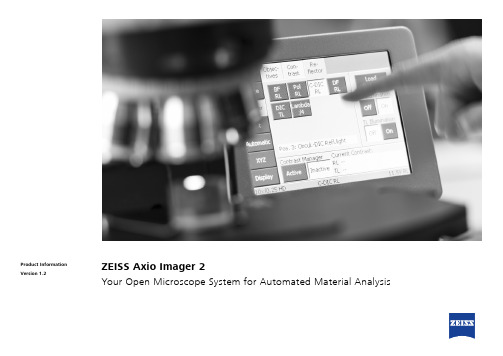
ZEISS Axio Imager 2Your Open Microscope System for Automated Material AnalysisProduct Information Version 1.2Axio Imager 2 from ZEISS is your system platform tailored to demanding materials analysis tasks, development of new materials as well as quality control.You always profit from crisp images and high optical performance. This applies in particular to sophisticated contrasting techniques, e.g. like the Circular Differential Interference Contrast (C-DIC) and polarization contrast.Use the motorized stand to achieve reproducible illumination settings and, consequently, constant image quality. You always obtain comparable results and high productivity by automating your workflow. Axio Imager 2 offers a high degree of adaptability in line with your future requirements. The stands are open to expand and cover a wide range of applications.Your Open Microscope System for Automated Material Analysis› In Brief › The Advantages › The Applications › The System› Technology and Details ›ServiceAnimation20 µmSimpler. More Intelligent. More Integrated.Profit from an Open Microscope System Whether in research, testing or failure analysis, materials microscopy faces quite various challenges. With Axio Imager 2 from ZEISS you will be able to meet and win these challenges. Attach application-specific components and perform e.g. particle analysis, investigate non-metallic inclusions (NMI), liquid crystals or semiconductor-based MEMs. Axio Imager 2 supports the correlative workflow to electron microscopic investigations, too.Achieve Reliable, Reproducible ResultsStability is essential if you want to obtain good results. You will appreciate the stable imaging conditions of Axio Imager 2, especially when working with high magnifications and performing time dependent studies. Due to the motorization of Axio Imager 2 you will achieve quick and repro-ducible results while you always work under constant conditions. For instance, the motorized apertures and the illumination control, which automatically adjusts the color temperature via filter wheels. Experience Competence in all Contrasting TechniquesChoose from a variety of contrasting techniques to achieve an optimum image quality for your dedicated applications. Examine your samples in reflected light in brightfield, darkfield, Differential Interference Contrast (DIC), Circular Differential Interference Contrast (C-DIC), polarization or fluorescence contrast. For transmitted light you can choose between brightfield, darkfield, Differential Interference Contrast (DIC), polarization or circular polarization. Minimized stray light enables homogenous illumination. You achieve outstanding image contrast, even at high magnifications.Carbon fiber-reinforced polymer (CFRP), Differential Interference Contrast (DIC); Objective: EC Epiplan-NEOFLUAR 50×/0.8Stage insert with correlative sample holder for a big variety of specimen.Appreciate the stable imaging conditions with Axio Imager 2.› In Brief› The Advantages › The Applications › The System› Technology and Details › ServiceBrightfield and Darkfield: Maximum Homogeneity and a Stray Light Free Image Background In brightfield Axio Imager 2 provides homoge-neous illumination and exceptional contrast. By minimizing disturbing stray light and reducing the longitudinal color aberration of the illumination optics, the darkfield illumination contrast is suitable for the most challenging samples and impresses even when faced with finest structures. Switching between the techniques only requires a simple turn. The motorized stands allow you to work particularly quickly and conveniently.C-DIC: Perfect for All StructuresCircular Differential Interference Contrast (C-DIC) is a polarization-optical technique which, in contrast to ordinary Differential Interference Contrast (DIC), uses circularly polarized light. This technique has a number of decisive advantages for the contrasting of differently aligned object structures. The speci-men no longer has to be rotated for best imageExpand Your PossibilitiesCopper casting, brightfield.Objective: EC Epiplan-NEOFLUAR 20×/0.5Copper casting, darkfield.Objective: EC Epiplan-NEOFLUAR 20×/0.5contrast and quality, as it is the case in basic DIC. With C-DIC it is simply enough to adjust the position of the C-DIC prism to achieve best image quality whether it is for contrast and/or resolution independent of sample orientation. And all this is possible using one C-DIC prism for a homoge-neous unsurpassed quality image.Copper casting, C-DIC.Objective: EC Epiplan-NEOFLUAR 20×/0.5Experience Competence in all Contrasting Techniques › In Brief› The Advantages › The Applications › The System› Technology and Details › Service200 µm Experience Competence in All Contrasting TechniquesExpand Your PossibilitiesBrightfieldDarkfieldC-DICSample: pure aluminum; Objective: EC Epiplan-NEOFLUAR 10×/0.25, same position acquired with different contrasting techniquesPolarization Contrast Polarization with Additional Lambda Plate› In Brief› The Advantages › The Applications › The System› Technology and Details › ServiceTailored Precisely to Your Applications› The Advantages› The Applications› The System› Technology and Details› ServiceTailored Precisely to Your Applications› The Advantages› The Applications› The System› Technology and Details› Service20 µm20 µm20 µm20 µm200 µm200 µmZEISS Axio Imager 2 at WorkAviation and Space IndustryCarbon fiber-reinforced polymer (CFRP), brightfield, objective: EC Epiplan-NEOFLUAR 50×/0.8Carbon fiber-reinforced polymer (CFRP), darkfield, objective: EC Epiplan-NEOFLUAR 50×/0.8Carbon fiber-reinforced polymer (CFRP), DIC, objective: EC Epiplan-NEOFLUAR 50×/0.8Raw iron, brightfield,objective: EC Epiplan-NEOFLUAR 50×/0.8Aluminium, polarization,objective: EC Epiplan-NEOFLUAR 10×/0.25Metal Producing and Processing IndustryAluminium, polarization with Lambda plate, objective: EC Epiplan-NEOFLUAR 10×/0.25› In Brief › The Advantages › The Applications › The System› Technology and Details › Service10 µm20 µm50 µmZEISS Axio Imager 2 at WorkOil, Gas and Mining IndustryVitrinite,objective: EC Epiplan-NEOFLUAR 50×/1.0 Oil PolCast iron, brightfield,objective: EC Epiplan-APOCHROMAT 50×/0.95Particle analysis, brightfield,objective: EC Epiplan-NEOFLUAR 20×/0.5Automotive IndustryParticle Analysis› In Brief › The Advantages › The Applications › The System› Technology and Details › ServiceExpand Your PossibilitiesAnalyze Tiny Particles: Accurately and ReproduciblyParticle Analyzer is a milestone for your quality control. With the fully motorized light microscope Axio Imager 2 you measure particles down to 2 µm.Particle Analyzer software supports the standards for cleanliness testing ISO 16232, VDA 19, and oil analysis ISO 4406, ISO 4407, and SAE AS 4059. With the system solutions from ZEISS, you ensure that the required microscope settings are always selected correctly. You receive reliable, reproducible results nearly independent of the user carrying out the analysis. By carrying out correlative particle analyzes, you expand the depth of information contained within your findings to include the results of element and materials characterization.› In Brief › The Advantages › The Applications › The System› Technology and Details › Service100 µmExpand Your PossibilitiesCompletely characterize residual dirt particles with Correlative Automated Particle Analysis from ZEISS. Detect particles with your Axio Imager 2 and relocate preselected particles automatically, using your SEM from ZEISS. Perform an EDX analyisis to reveal information of their elemental composition. Correlative Particle Analyzer automatically documents the results from both, the light microscopic and electron microscopic analysis. You receive a combined, informative report at the touch of a button.As an experienced user, you can inspect the results of the combined light microscopic and electron microscopic analysis on an interactive overview screen. Retrieve particles at the touch of a button, automatically start new EDX analyzes, and auto-matically generate a report. With Correlative Particle Analyzer, your results will be available up to ten times faster than first conducting an analysis with a light microscope and then sub-sequently with an electron microscope. You can systematically focus on potentially process-critical particles.The complementary material characterization from both microscopic worlds gives you added security.Correlative Automated Particle Analysis (CAPA): More Knowledge. Higher Quality.Image of a metallic particle from a light microscopeImage of the same metallic particle from an electron microscopeOverlay of the images from both systems; chemical element composition via EDX analysis; graphical EDX overlay prepared with Bruker Esprit softwareCorrelative sample holder for efficient relocation of particles in your ZEISS scanning electron microscope.› In Brief › The Advantages › The Applications › The System› Technology and Details › Service20 µm 20 µm20 µm20 µmExpand Your PossibilitiesCLEM (Correlative Light and Electron Microscopy) image of a region of interest from an aged Li-ion battery with different contrasts of brightfield (a) and polarized light (b) in LM as well as BSE signal (c) and EDS mapping (d) in SEM.Correlative Microscopy withZEISS Axio Imager 2: Bridging the Micro and Nano WorldAre you looking for a way to combine imaging and analytical methods effectively?Shuttle & Find offers precisely this: An easy-to-use, highly productive workflow from a light to an electron microscope – and vice versa.The workflow between the two systems has never been so easy. The precise recall of regions of interest enhances productivity. Instead of wasting valuable time searching, you now gain new insights into your samples with a few mouse clicks. Regions of interest, marked on one system, you can instantely relocate on the other system. Open up new dimensions of information in numerous material analysis applications. Absolutely reproducible.› In Brief › The Advantages › The Applications › The System› Technology and Details › ServiceExpand Your PossibilitiesExaminations in the fields of research and industrial production (e.g. surface examinations of reflective, low-contrast specimens such as metallographic specimens and polished or textured wafers) require a fast focusing system that ensures high precision levels of max. 0.3 times the objective’s depth of field. This requirement can be easily met by com-bining your Axio Imager 2 with the Auto Focus system to benefit from fast and accurate focusing across a wide capture range of up to 12,000 µm. The Auto Focus system is designed to work with reflected light and transmitted light in brightfield, darkfield, polarized light and DIC.How it WorksThe objective guides the structured light produced by an LED in the Auto Focus system onto the specimen, with the specimen’s surface reflecting it back. During this process, Auto Focus permanently analyses the signal and derives the appropriate control signals for the focus drive, to bring the surface into focus. The Auto Focus sensor detects changes and deviations in the focus position and compensates them automatically. The Auto Focus system comes with three different modes corre-sponding to different specimen characteristics (reflective/partially reflective/diffuse) and with three different precision levels (precision/balance/speed).How the Auto Focus system works: 1) LED 2) Sensor module 3) Sensor 4) Beam splitter 5) O bjective 6) Specimen› In Brief › The Advantages › The Applications › The System› Technology and Details › Service5362141 Microscope• Axio Imager.A2m (encoded)• Axio Imager.D2m (encoded, partly motorizable)• Axio Imager.M2m (motorizable, TL manual)• Axio Imager.Z2m (motorizable, TL motorized)2 Objectives Reflected Light • EC EPIPLAN• EC Epiplan-NEOFLUAR • EC Epiplan-APOCHROMAT Transmitted Light • N-ACHROPLAN • EC Plan-NEOFLUAR • Plan-APOCHROMAT • C-APOCHROMAT • FLUARLong Working Distance • LD EPIPLAN• LD EC Epiplan-NEOFLUAR 3 Illumination Reflected Light • MicroLED • VisLED • Halogen • HBO / HXP Transmitted Light • MicroLED • VisLED • HalogenYour Flexible Choice of Components4 Cameras • Axiocam 105 • Axiocam 305• Axiocam 506• Axiocam 705• Axiocam 7125 Software • ZEN core • ZEN starter6 Accessories • Auto Focus• Linkam heating- and cooling stages • Focus Linear Sensor • Correlative Microscopy› In Brief › The Advantages › The Applications › The System› Technology and Details › ServiceSystem Overview› The Advantages› The Applications› The System› Technology and Details› ServiceSystem Overview› The Advantages› The Applications› The System› Technology and Details› ServiceSystem Overview› The Advantages› The Applications› The System› Technology and Details› ServiceTechnical Specifications› The Advantages› The Applications› The System› Technology and Details› ServiceTechnical Specifications› The Advantages› The Applications› The System› Technology and Details› ServiceTechnical Specifications› The Advantages› The Applications› The System› Technology and Details› ServiceTechnical Specifications› The Advantages› The Applications› The System› Technology and Details› ServiceBecause the ZEISS microscope system is one of your most important tools, we make sure it is always ready to perform. What’s more, we’ll see to it that you are employing all the options that get the best from your microscope. You can choose from a range of service products, each delivered by highly qualified ZEISS specialists who will support you long beyond the purchase of your system. Our aim is to enable you to experience those special moments that inspire your work.Repair. Maintain. Optimize.Attain maximum uptime with your microscope. A ZEISS Protect Service Agreement lets you budget for operating costs, all the while reducing costly downtime and achieving the best results through the improved performance of your system. Choose from service agreements designed to give you a range of options and control levels. We’ll work with you to select the service program that addresses your system needs and usage requirements, in line with your organization’s standard practices.Our service on-demand also brings you distinct advantages. ZEISS service staff will analyze issues at hand and resolve them – whether using remote maintenance software or working on site. Enhance Your Microscope System.Your ZEISS microscope system is designed for a variety of updates: open interfaces allow you to maintain a high technological level at all times. As a result you’ll work more efficiently now, while extending the productive lifetime of your microscope as new update possibilities come on stream.Profit from the optimized performance of your microscope system with services from ZEISS – now and for years to come.Count on Service in the True Sense of the Word>> /microservice› In Brief › The Advantages › The Applications › The System› Technology and Details › ServiceCarl Zeiss Microscopy GmbH 07745 Jena, Germany******************** /axioimager-mat Notfortherapeuticuse,treatmentormedicaldiagnosticevidence.Notallproductsareavailableineverycountry.ContactyourlocalZEISSrepresentativeformoreinformation.EN_42_11_31|CZ11-219|Design,scopeofdelivery,andtechnicalprogresssubjecttochangewithoutnotice.|©CarlZeissMicroscopyGmbH。
stable difusion api img2img 参数

stable difusion api img2img 参数简介在计算机视觉领域,图像转换是一个重要的任务。
图像间的转换可以用于图像修复、风格转换、图像增强等多个应用场景。
而在实际应用中,我们更倾向于使用稳定性好、效果好的图像转换算法。
而 stable difusion api img2img 就是一个强大的图像转换模型。
什么是 stable difusion api img2img?stable difusion api img2img 是一个基于稳定扩散(Stable Difusion)算法的图像转换模型。
它是由图像中心切块、转化为低维潜变量、通过正反向映射进行转换的一种方法。
这个模型可以在图像转换任务中取得很好的效果,并且具有较高的稳定性,适用于各种图像转换应用。
稳定扩散算法简介稳定扩散算法是一个基于梯度迭代的图像转换方法。
它的主要思路是将图像转换问题转化为一个梯度下降问题,通过迭代优化潜变量,从而实现图像的转换。
稳定扩散算法的具体步骤如下: 1. 图像切块:将输入的图像按照一定的尺寸进行切块,得到一系列的小图像块。
2. 特征提取:使用深度神经网络对每个小图像块进行特征提取,得到对应的低维潜变量。
3. 正向映射:使用正向映射函数将低维潜变量映射到目标图像的低维潜变量空间。
4. 反向映射:使用反向映射函数将目标图像的低维潜变量映射回原始图像空间。
5. 梯度下降:通过梯度下降算法迭代优化潜变量,从而不断改进图像转换的效果。
6. 重构图像:在达到一定的迭代次数后,将更新后的潜变量反向映射回原始图像空间,得到最终的转换结果。
stable difusion api img2img 的参数设置为了实现更好的图像转换效果,stable difusion api img2img 提供了多个参数供用户设置。
以下是一些重要的参数: 1. image_size:输入图像的大小。
2. latent_dim:潜变量的维度。
stable diffusion img2img原理

stable diffusion img2img原理一、引言本文将详细介绍stable diffusion img2img原理。
img2img是一种图像到图像的转换方法,它可以将一张图像转换为另一张图像,广泛应用于计算机视觉、图像处理等领域。
stable diffusion作为一种稳健的扩散算法,具有稳定、高效的优点,可以应用于多种img2img 任务中。
二、原理概述1. 扩散过程:在img2img转换中,扩散是一种常用的方法,它可以将输入图像逐步转换为目标图像。
在stable diffusion算法中,通过将原始图像和噪声图像进行迭代处理,逐渐向目标图像方向演变。
2. 稳定扩散:stable diffusion算法采用了一种稳定扩散机制,通过在每次迭代中引入一些随机噪声,使得算法在处理不同输入图像时都能够得到稳定的结果。
这种机制能够避免算法陷入局部最优解,从而提高算法的鲁棒性和稳定性。
3. 权重更新:在stable diffusion算法中,通过更新每个像素的权重来实现图像的转换。
权重更新规则采用了一种非线性函数,能够根据像素值的大小自动调整权重,从而实现平滑过渡的效果。
这种权重更新规则可以确保算法在处理不同输入图像时都能够得到较为自然的图像转换效果。
三、步骤详解1. 初始化:首先,需要将原始图像和噪声图像进行初始化,并设置一定的迭代次数。
2. 迭代处理:在每次迭代中,将原始图像与噪声图像进行卷积操作,并更新每个像素的权重。
重复以上步骤,直到达到预设的迭代次数或达到满意的转换效果。
3. 后处理:在迭代完成后,对转换后的图像进行一些后处理操作,如阈值化、色彩调整等,以得到更加自然和清晰的图像转换效果。
四、应用场景stable diffusion算法可以应用于多种img2img任务中,如人脸识别、图像修复、超分辨率等。
通过将输入图像转换为目标图像,可以提高图像的质量和清晰度,为计算机视觉和图像处理领域的研究和应用提供了有力支持。
stable diffusion img2img 参数

"Stable Diffusion" 是一种深度学习模型,通常用于图像到图像的转换。
它经常被用于图像修复、超分辨率、风格迁移等任务。
至于"img2img" 参数,这通常是指在深度学习中使用的图像到图像转换任务的参数。
在 Stable Diffusion 中,img2img 参数可能包括以下几种:
1. **输入图像大小**:这指的是输入到模型的图像的大小。
通常,这会是一个二维的元组,例如 (256, 256)。
2. **步长**:这指的是在扩散过程中,每个步骤中随机噪声的添加量。
步长越大,噪声的添加量就越多,反之亦然。
3. **时间步长**:这指的是在扩散过程中,每个步骤之间的时间间隔。
时间步长越大,每个步骤之间的间隔就越长。
4. **学习率**:这指的是在训练过程中,模型参数更新的步长。
学习率越大,参数更新的步长就越大,反之亦然。
5. **权重衰减**:这指的是在训练过程中,对模型参数施加的权重衰减。
权重衰减越大,模型参数的权重就越小。
6. **批次大小**:这指的是在训练过程中,每次更新模型参数时使用的样本数量。
批次大小越大,每次更新的样本数量就越多。
7. **迭代次数**:这指的是在训练过程中,模型参数更新的总次数。
迭代次数越多,模型参数更新的次数就越多。
这些参数通常需要根据具体任务和数据集进行调整和优化。
- 1、下载文档前请自行甄别文档内容的完整性,平台不提供额外的编辑、内容补充、找答案等附加服务。
- 2、"仅部分预览"的文档,不可在线预览部分如存在完整性等问题,可反馈申请退款(可完整预览的文档不适用该条件!)。
- 3、如文档侵犯您的权益,请联系客服反馈,我们会尽快为您处理(人工客服工作时间:9:00-18:30)。
Examples of Motion Fields I
(a)
(b)
(a) Motion field of a pilot looking straight ahead while approaching a fixed point on a landing strip. (b) Pilot is looking to the right in level flight.
The matrix for corner detection:
TA) (A
is singular (not invertible) when det(ATA) = 0 But det(ATA) = ∏ λi = 0 -> one or both e.v. are 0 One e.v. = 0 -> no corner, just an edge Two e.v. = 0 -> no corner, homogeneous region Aperture Problem !
Segmentation Problem
– What are the regions of the image plane which correspond to different moving objects?
Motion Field (MF)
The MF assigns a velocity vector to each pixel in the image. These velocities are INDUCED by the RELATIVE MOTION btw the camera and the 3D scene The MF can be thought as the projection of the 3D velocities on the image plane.
E ( x + uδt , y + vδt , t + δt ) = E ( x, y, t )
Taylor expansion
E E E + e = E ( x, y , t ) + δy + δt t x y dividing by δt and taking limit δt → 0 E ( x , y , t ) + δx
– Camera still, moving scene – Moving camera, still scene – Moving camera, moving scene
Motion Analysis Problems
Correspondence Problem
– Track corresponding elements across frames
Brightness Constancy Equation
Let P be a moving point in 3D:
– At time t, P has coords (X(t),Y(t),Z(t)) – Let p=(x(t),y(t)) be the coords. of its image at time t. – Let E(x(t),y(t),t) be the brightness at p at time t.
– The summations are over all pixels in the K x K window
Taking a closer look at
TA) (A
This same matrix can be used for corner detection!
Taking a closer look at
vxLeabharlann The OF is CONSTRAINED to be on a line !
Interpretation
Values of (u, v) satisfying the constraint equation lie on a straight line in velocity space. A local measurement only provides this constraint line (aperture problem). Normal flow u n
The aperture problem
Aperture Problem
(a)
(b)
(a) Line feature observed through a small aperture at time t. (b) At time t+δt the feature has moved to a new position. It is not possible to determine exactly where each point has moved. From local image measurements only the flow component perpendicular to the line feature can be computed. Normal flow: Component of flow perpendicular to line feature.
(E
x
, E y ) (u , v ) = Et
Let n =
(E E ) (E , E )
x y x y
T T
E E E y Et u n = (u n )n = 2 x t , 2 E +E E +E 2 y x y x
T
Optical flow equation
Barber Pole illusion /Ambiguous/barberpole.htm
Brightness Constancy Assumption:
– As P moves over time, E(x(t),y(t),t) remains constant.
Brightness Constraint Equation
Let E ( x, y, t ) be the irradiance and u ( x, y ), v( x, y ) the components of optical flow.
Reconstruction Problem
– Given a number of corresponding elements, and camera parameters, what can we say about the 3D motion and structure of the observed scene?
Brightness Constancy Equation
Let
(Frame spatial gradient)
(optical flow)
and
(derivative across frames)
Brightness Constancy Equation
Becomes:
vy E -Et/| E|
– If we use a 5x5 window, that gives us 25 equations per pixel!
Constant flow
Prob: we have more equations than unknowns
Solution: solve least squares problem – minimum least squares solution given by solution (in d) of:
Optical flow field: apparent motion of brightness patterns We equate motion field with optical flow field
2 Cases Where this Assumption Clearly is not Valid
Solving the aperture problem
How to get more equations for a pixel?
– Basic idea: impose additional constraints
most common is to assume that the flow field is smooth locally one method: pretend the pixel’s neighbors have the same (u,v)
Examples of Motion Fields II
(a)
(b)
(c)
(d)
(a) Translation perpendicular to a surface. (b) Rotation about axis perpendicular to image plane. (c) Translation parallel to a surface at a constant distance. (d) Translation parallel to an obstacle in front of a more distant background.
E dx E dy E + =0 + x dt y dt t which is the expansion of the total derivative dE =0 dt short: E x u + E y v + Et = 0
Brightness Constancy Equation
Taking derivative wrt time:
Assuming that illumination does not change: Image changes are due to the RELATIVE MOTION between the scene and the camera. There are 3 possibilities: