Correlation Between BATSE Hard X-ray Spectral and Timing Properties of Cygnus X-1
grey correlation analysis
Grey Correlation AnalysisIntroductionGrey correlation analysis is a statistical method used to measure the correlation between two or more variables when the data is limited or uncertain. It was developed by Deng Julong in China in the 1980s and has since been widely applied in various fields including finance, economics, engineering, and social sciences.Grey correlation analysis is particularly useful when dealing with incomplete or uncertain data. It can provide valuable insights and helpin decision-making processes when traditional correlation analysis methods may not be applicable.Principles of Grey Correlation AnalysisGrey correlation analysis is based on the principles of grey system theory, which aims to study systems with limited information and uncertain data. The method involves four main steps:1.Data Organization: The first step in grey correlation analysis isto organize the available data. This may involve collecting datafrom various sources and arranging it in a systematic manner.2.Data Comparison: Once the data is organized, the next step is tocompare the different variables or factors under consideration.This can be done using various statistical measures such as mean,range, and standard deviation.3.Grey Correlation Coefficient Calculation: The grey correlationcoefficient is calculated to measure the correlation between thevariables. It is a value between 0 and 1, where a higher valueindicates a stronger correlation. The grey correlation coefficient takes into account the uncertainties and variations in the data.4.Grey Correlation Analysis: Finally, the grey correlation analysisis performed to determine the relationships between the variables.This can help in identifying the most influential factors andmaking predictions or forecasts based on the available data.Applications of Grey Correlation AnalysisGrey correlation analysis has been widely used in various fields for different purposes. Some of the applications include:1. Financial AnalysisGrey correlation analysis has been applied in financial analysis to study the relationships between different financial indicators. It can help in identifying the key factors influencing the financial performance of companies or investment portfolios. For example, it can be used to analyze the correlation between stock prices and economic indicators such as inflation rates or interest rates.2. Engineering DesignIn engineering design, grey correlation analysis can be used to evaluate the relationship between various design parameters and the performance of a system or product. It can help in optimizing the design process by identifying the most critical factors and their impact on the overall performance. For example, it can be used to analyze the correlation between different manufacturing parameters and the strength of a material.3. Economic ForecastingGrey correlation analysis has also been used in economic forecasting to predict future trends based on historical data. It can help in identifying the key factors influencing economic growth or decline and making accurate predictions. For example, it can be used to analyze the correlation between GDP growth and factors such as consumer spending, investment, and government policies.4. Social SciencesIn social sciences, grey correlation analysis can be used to study the relationships between different social or demographic variables. It can help in understanding the factors influencing social phenomena and making informed policy decisions. For example, it can be used to analyze the correlation between education levels, income levels, and crime rates in a specific region.Advantages and LimitationsGrey correlation analysis has several advantages over traditional correlation analysis methods. Some of the advantages include:•Suitable for limited or uncertain data: Grey correlation analysis can handle situations where the data is incomplete or uncertain,making it useful in real-world applications.•Provides insights in complex systems: Grey correlation analysis can provide valuable insights in complex systems where traditional correlation analysis methods may not be effective.•Helps in decision-making: Grey correlation analysis can help in decision-making processes by identifying the most influentialfactors and their impact on the outcomes.However, grey correlation analysis also has some limitations. These include:•Subject to data quality: The accuracy and reliability of the results obtained through grey correlation analysis are highlydependent on the quality of the data used.•Limited to linear relationships: Grey correlation analysis assumesa linear relationship between the variables under consideration.It may not be suitable for analyzing non-linear relationships.•Interpretation challenges: Interpreting the results of greycorrelation analysis can be challenging due to the complexity ofthe method and the uncertainties involved.ConclusionGrey correlation analysis is a valuable statistical method for measuring the correlation between variables when data is limited or uncertain. It has been widely applied in various fields and has provided valuable insights in complex systems. However, it is important to consider the limitations and challenges associated with grey correlation analysis when using it for decision-making processes. Overall, grey correlation analysis is a useful tool that complements traditional correlation analysis methods and helps in addressing real-world challenges.。
外源性磷输入改变农业河岸带湿地中土壤溶解有机碳的复杂性

Exogenous phosphorus inputs alter complexity of soil-dissolved organic carbon in agricultural riparianwetlandsMeng Liu a ,Zhijian Zhang a ,⇑,Qiang He b ,Hang Wang a ,Xia Li a ,Jonathan Schoer caCollege of Natural Resource and Environmental Sciences,China Academy of West Region Development,ZheJiang University,Yuhangtang Avenue 866,HangZhou,ZheJiang Province 310058,China bDepartment of Civil and Environmental Engineering,University of Tennessee,Knoxville,TN 37996-2010,USA cDepartment of Chemistry,Valparaiso University,Valparaiso,IN 46383,USAh i g h l i g h t sExternal P input stimulated the production of sediment active C fractions.External P input decreased DOC humicity and increased its microbial-derived sources. Sediments with gradient P loading rate had a blue shift of fluorescence fingerprint. Spectra measurements were helpful for describing sediment DOC composition.a r t i c l e i n f o Article history:Received 29June 2013Received in revised form 23September 2013Accepted 25September 2013Available online 30October 2013Keywords:Dissolved organic carbon (DOC)Phosphorous (P)Riparian wetlandsStructural compositiona b s t r a c tHigh-strengthened farmland fertilization leads to mass inputs of nutrients and elements to agricultural riparian wetlands.The dissolved organic carbon (DOC)of such wetland sediments is an important inter-mediate in global carbon (C)cycling due to its role in connecting soil C pools with atmospheric CO 2.But the impact of phosphorus (P)on sediment DOC is still largely unknown,despite increasing investigations to emphasize P interception by riparian wetlands.Here,we simulated the temporal influences of exoge-nous P on sediment DOC of riparian wetlands by integrating gradient P loading at rates of 0%,5%,10%,20%,30%,and 60%relative to the initial total phosphorus content of the sediment with the purpose of illustrating the role of external P on the complexity of soil DOC in terms of its amount and composition.After incubating for nine months,a dramatic linear correlation between Olsen-P and fluorescent and ultraviolet spectral indices considered DOC skeleton was observed.Together with a more microbial-derived origin of DOC and a reduction of DOC aromaticity or humicity,the excitation-emission matrix had shown a blue shift reflecting a trend towards a simpler molecular structure of sediment DOC after P addition.Meanwhile,the content of soil DOC and its ratio with total organic carbon (TOC)were also increased by P loading,coupled with enhanced values of highly labile organic carbon and two C-related enzymes.While TOC and recalcitrant organic carbon decreased significantly.Such implications of DOC amounts and composition stimulated by external P loading may enhance its bioavailability,thereby inducing an accelerated effect on soil C cycling and a potential C loss in response to global climate change.Ó2013Elsevier Ltd.All rights reserved.1.IntroductionSince the 1980s,as agricultural activity has intensified signifi-cantly in Eastern China,the extensive application of fertilizers to farmlands and production of livestock manure have led to great phosphorus (P)loss from agricultural areas to adjacent ecosystems (Zhang and Shan,2008).Enhanced levels of P not only have led to great eutrophication with characteristic algal blooms (Roberts et al.,2012),but have also impacted the ecological remediationand resilience of such aquatic ecosystems (Jeppesen et al.,2005;Wang et al.,2013).For this particular purpose,many riparian wet-lands have been arranged in agricultural catchments in use world-wide to reduce the concentration of nutrients in through-flowing water and improve water quality (Verhoeven et al.,2006;Hoff-mann et al.,2009).Currently,total phosphorus (TP)content in riparian wetland sediment located in the southern region of the Taihu Basin has reached 169–1200mg kg À1after interception (Wang et al.,2010).Some researchers have found the decomposi-tion of longer-term or mineral-associated soil carbon (C)fractions and soil organic C sink strengths could be enhanced by P availability (Mack et al.,2004;Cleveland and Townsend,2006;0045-6535/$-see front matter Ó2013Elsevier Ltd.All rights reserved./10.1016/j.chemosphere.2013.09.117Corresponding author.Tel.:+8657186971854;fax:+8657186971719.E-mail addresses:zhangzhijian@ (Z.Zhang),qhe2@ (Q.He).Bradford et al.,2008).Other authors pointed out that undesired ef-fects such as additional risks for global warming may be induced as a result of nutrients overloading wetland sediment(Verhoeven et al.,2006;Zhang et al.,2012;Wang et al.,2013).However,the is-sue of sediment P accumulation on the sediment C pool has at-tracted less attention during past years,while policymakers mostly focus on the interception of P in riparian wetlands.Global warming significantly correlates to CO2loss from soils and creates a feedback to oceanic and land ecosystems(Cox et al.,2011).In soils,dissolved organic carbon(DOC),as the impor-tant fraction in the active soil organic C pool(Song et al.,2012), intimately correlates with CO2evolution from soil although DOC makes up only a small portion of total soil organic matter(Fang and Moncrieff,2005;Bengtson and Bengtsson,2007;Zhao et al., 2008).Meanwhile,soil DOC not only contains both substrates and end products of enzymatic reactions of varying molecular weight,but also constitutes the most bioavailable moiety for soil microorganisms(Song et al.,2012).Some researchers have also found that soil microbial respiration is significantly limited by large differences in the complexity of DOC(Fang and Moncrieff, 2005).Moreover,the microbial degradability of DOC and,there-fore,the relationship with C mineralization from soils may also be affected by its composition(Zhao et al.,2008),although not al-ways linearly dependent in amounts(Liu et al.,2012).The features of the DOC skeleton,particularly percent aromaticity,degree of structural conjugation,and humicity(Johnson et al.,2011;Guo et al.,2013),are of fundamental significance to indicating the retention or out-gassing processes for soil C pools(Wilson and Xenopoulos,2008).For instance,aromatic compounds probably derived from lignin are stable components,whereas carbohydrates are preferentially respired(Kalbitz et al.,2003).Thus,connecting DOC content variance with its structural complexity would better reflect the status and bioavailability of the soil C pool and its fur-ther retention.Among analytical characterization methods,the ra-pid,non-destructive,cost-effective,and informative density nature offluorescence spectroscopy(Guo et al.,2013)is well suited to provide informative data on the aromatic content and humicity of DOC,specific locations of differentfluorophores,andfluorescent characteristics of structure,functional group,configuration,heter-ogeneity,and molecular dynamics,which gives information about DOC composition(Fellman et al.,2008;Johnson et al.,2011;Guo et al.,2013).In soils,environmental factors such as climate(tem-perature,precipitation)and vegetation,or anthropic disturbances such as land-use,acidification,tillage,and application of fertilizer, may affect the DOC amount and composition indirectly via micro-bial consumption and lysis(Hishi et al.,2004;Jinbo et al.,2006). However,until recently,few studies have focused on the impacts of external P amendment on DOC of agricultural riparian wetland sediment,both in amount and composition,and thus the underly-ing mechanisms are largely unknown.Obviously,it is important to investigate the impact of P addition on wetland sediment DOC amounts,as well as its composition in agricultural areas.In this study,we designed a simulative experi-ment to illustrate the complex status of DOC by conducting labora-tory-scale incubation with P addition at rates of0%(P-0),5%(P-5), 10%(P-10),20%(P-20),30%(P-30),and60%(P-60)relative to the initial TP content of the sediment(0.29g kgÀ1;Supplementary Information,SI-1).Fluorescent and ultraviolet(UV)spectral mea-surements directly describe the effect on soil DOC composition. Moreover,the use of chemical or biochemical tests,with respect to their relationships withfluorescent and UV indices,gives in-sights into the complexity and biological degradability of soil DOC under disturbance of P inputs will be discussed.Further,we hypothesize that P loading could induce the variance of sediment DOC amount and composition to that of a simpler molecular struc-ture and enhance the bioavailability of soil DOC,thereby leading to a weakening effect on potential retention processes of soil C pool and accelerate soil C cycling in response to climate changes.2.Material and methods2.1.Site description and experimental designsRiparian wetland soil samples for this study were collected from the Southwest part of the Taihu Lake Basin(30°18051.8400N and119°54013.3700E).This area is one of the most productive and intensively farmed agricultural areas in the downstream delta re-gion of the Yangtze River in Southeast China.This region possesses a subtropical monsoon climate with an average summer tempera-ture of28°C and an average annual rainfall of1550mm.The most common agricultural land uses in this area include ricefields,veg-etable gardens,aquaculture,and swine farms.During the pastfive years,the annual soil P application rate has been30–85kg haÀ1-yrÀ1.In order to best profile the impact of exogenous P on soil DOC features,sediment was selected from a site(pH7.24;mois-ture57%)that contained a relatively low initial TP concentration of0.29g kgÀ1,compared to other similar wetland sediments in this region(0.17–1.20g kgÀ1of TP)(Wang et al.,2010).An average water depth around this particular sampling riparian wetland was1.4m with macrophyte plants on bank,and there was no arti-ficial channel existing nearby this natural isolated pond.The or-ganic C of this riparian wetland stored in the sediment and no other C inputs in this region,and the basic properties of the wet-land sediment were provided in Table2.The sediment samples were collected using a lab-made stain-less steel sampler at a depth of0–10cm from20different points. Samples were wiped clear of macro-particles and transported on ice to the lab within3h after collection.Plastic barrels(35cm diameterÂ35cm height)werefilled with8kg of mixed wet soil (5kg dry weight)to a depth of20cm.Water-soluble superphos-phate(CaP2H4O8)was chosen to be the external P in our study, which was recognized by Justus Liebig as P-related fertilizer and applied widely to agricultural production(Brunner,2010).Super-phosphate of different mass was dissolved with deionized water, then the mixed solution was added to those soil-filled barrels homogeneously with a spray without disturbing soil cores,of which TP concentration accounted for0%(P-0),5%(P-5),10% (P-10),20%(P-20),30%(P-30),and60%(P-60)relative to the initial sediment TP content.See supplementary information(SI-1)for the rationale for selecting the spiking levels of P in the sediment sam-ples.After several minutes,all the samples were covered with a 10cm layer of deionized water and were incubated in the labora-tory.To avoid the growth of aquatic plants and disturbance from other environmental factors,the barrels were placed in lab with dam-board to keep the samples in the dark at room temperature (20–25°C)for the nine months incubation.Deionized water was replenished every three months to maintain the liquid depth.Trip-licates of each sample were prepared.2.2.Soil samplingSoil samples for multifarious analyses were collected after incu-bating them for nine months.Each barrel was divided into four sub-barrels to minimize edge effects for grab-sampling.The soil samples for each barrel consisted of four composited2cm diame-terÂ10cm deep cores.50g fresh soil was collected from each bar-rel and then divided into two aliquots.One aliquot was stored at 4°C in the dark for microbial biomass and enzyme studies while the other was air-dried and ground to pass through a1mm mesh sieve for subsequent chemical analyses and spectral measurements.M.Liu et al./Chemosphere95(2014)572–5805732.3.Analytical methods2.3.1.Spectral measurementsBased on reported methods(Wilson and Xenopoulos,2008;Guo et al.,2013),the Solutions for UV andfluorescence measurements to determine DOC structure were prepared by water extraction of the air-dried and sieved(100mesh sieves)soil in a1:5w/w ratio to Milli-Q water,then shaking for4h at room temperature.Extracts were centrifuged at7000rpm(Hitachi Inc.,CR22G,Japan)for 10min at4°C andfiltered through a0.45l m membranefilter. The quantity of DOC in the extract was measured with a total or-ganic carbon(TOC)analyzer(Shimadzu Inc.,TOC-VCHP,Japan).Four UV andfluorescence–related indices were determined in this study:fluorescence index(FI),humification index(HI),fresh-ness index(b/a),and specific UV absorbance at280nm(E280).De-tails about the determination of these indices are provided in the supplementary information(SI-2).Briefly,FI,b/a,and HI were determined using afluorescence spectrophotometer(Hitachi Inc., F-4500,Japan).While E280was determined using a UV scanning spectrophotometer(Shimadzu Inc.,UV-2550,Japan).Milli-Q high-purity water was used as the reference for all measurements. Spectralfluorometric3D excitation-emission matrix(EEM)mea-surements were obtained for excitation wavelengths from200to 400nm and at emission wavelengths from300to600nm at 5nm increments as previously described(Wilson and Xenopoulos, 2008).Data analysis was then performed using an in-house pro-gram SigmaPlot12.0.2.3.2.Chemical and biochemical analysisMeasurements of sediment TOC,DOC,TP,and available P(pH 8.5,0.5mol LÀ1NaHCO3extractable P,i.e.,Olsen-P)were con-ducted according to standard methods of physicochemical analysis (ISSCAS,1978;Westerman,1990).Due to the susceptibility of or-ganic C to KMnO4oxidation,the contents of three fractions of labile organic components in soil samples,namely highly labile organic carbon(HLOC),mid-labile organic carbon(MLOC),and labile or-ganic carbon(LOC),were determined using33,167,and 333mmol LÀ1KMnO4,respectively(Loginow et al.,1987).Recalci-trant organic carbon(ROC)was calculated as the difference be-tween these three labile C forms and the TOC.Soil microbial biomass C(MBC)and P(MBP)were determined by the chloroform fumigation extraction method(Inubushi et al.,1991).Moist soil samples were split into two subsamples with one immediately ex-tracted with either0.5mol LÀ1K2SO4for MBC or0.5mol LÀ1 NaHCO3for MBP,while the other was fumigated with chloroform and then extracted.Following centrifugation,C and P concentra-tions of soil microbial biomass were calculated from the difference between the fumigated and non-fumigated soil samples.2.3.3.Enzyme analysisThree eco-enzymes,b-1,4-glucosidase(BG),cellobiohydrolase (CBH),and acid phosphatase(AP)(Sinsabaugh et al.,2009)were se-lected as indicators of microbial nutrient demand in the C and P cy-cles,respectively.Sample suspensions were prepared by using a vortex mixer for1min to homogenize1g(wet weight)of soil with 125mL of50mmol LÀ1sodium acetate buffer(pH6.0to match the mean soil pH of the environmental samples).Sample suspensions, buffer,references,and substrates(the substrate solutions for BG, CBH and AP are4-MUB-b-D-glucoside,4-MUB-b-D-cellobioside, and4-MUB-phosphate,respectively)were pipetted into96-well blankfluorescent plates(Corning Inc.,costar3603,USA)following the strict order and position on the well plate according to the work of Saiya-Cork(Saiya-Cork et al.,2002).The micro-plates were covered and incubated in the dark at20°C for4h.Then,10l L of 1.0mol LÀ1NaOH was added to each well to stop the reaction and increase thefluorescence of residual substrates.Finally,standard high-throughputfluorometric detection of the enzyme assays were carried out using a Bio-Tek Synergy HT microplate reader(Bio-Tek Inc.,Winooski,VT,USA)with365nm excitation and460nm emissionfilters(Saiya-Cork et al.,2002).Enzyme activities were calculated and expressed as nmol hÀ1gÀ1(Sinsab-augh et al.,2008).2.4.Statistical analysisData were tested for homogeneity of group variances using the Pearson test.Data were square root transformed if necessary.The data were analyzed by analysis of variance using SPSS16.0statis-tical software.For the enzymes analysis,each data point was char-acterized by a response ratio(RR)and the log of the response ratio (L RR).RR was calculated as the mean of the experimental samples divided by the mean of the control samples(sample P-0)to provide an index of response magnitudes,while L RR was calculated as the log10of RR.The use of L RR is preferred over the use of RR because it equally weighs the negative and positive responses and facili-tates statistical analysis(Marklein and Houlton,2012).Positive values of L RR represented an increase in enzyme activity relative to the control sample,whereas negative values indicated sup-pressed activity.Before analysis,each class was summarized by the weighted mean of L RR(LÃRR).3.Results3.1.Structural complexity of soil DOC under phosphorus loadingSpectral analysis showed that P input was an excellent factor for soil DOC composition of the riparian wetlands(Table1).FI in soil solutions was raised from P-0to P-60by a range of0.65%to a max-imum6.5%.Meanwhile,the ratio of b/a was observed to follow the same trend as FI,with an increment of21–64%.As to aromatic sub-strate,E280and HI were reduced in all P loading samples by a fac-tor of3–12%and12–47%,respectively.Moreover,we found that all spectral indices changed significantly with P availability.Briefly,FI and b/a correlated positively with Olsen-P content(Fig.1A and C; p<0.05),but the relationship with respect to HI was negative (Fig.1D;p<0.05),while there existed a less linear correlation with E280(Fig.1B).Two remarkablefluorophores in3D EEMs were revealed from the tested six treatments:one at Ex/Em280–320/ 400–450nm and another at Ex/Em210–240/395–450nm(Fig.2). Usually,the peak at longer wavelengths was recognized as the humic-likefluorescence peak C in the UV region,while the other was determined to be the humic-like peak A in the visible region (Klotzbücher et al.,2012).Compared to humic-likefluorophores reported in Fig.2,a clear blue shift about the positions of the fluorophores both in the visible and UV region was observed with the increment of P loading,displaying a trend towards shorterTable1Spectral parameters of sediment dissolved organic carbon(DOC)in the tested samples,namelyfluorescence index(FI),humification index(HI),UV absorption at 280nm(E280),and freshness index(b/a).Treatment FI E280b/a HIP-0 1.53±0.05b0.63±0.08ab0.91±0.07cd0.48±0.01a P-5 1.54±0.01b0.64±0.03a0.88±0.08d0.42±0.01b P-10 1.56±0.02ab0.61±0.03ab0.90±0.03cd0.40±0.03b P-20 1.59±0.03ab0.56±0.01ab 1.00±0.06c0.32±0.01c P-30 1.59±0.05ab0.55±0.03b 1.31±0.02b0.22±0.01d P-60 1.63±0.07a0.57±0.02ab 1.49±0.03a0.22±0.01d Values in parentheses are standard deviations.Different letters listed beside the data represent significant differences at p<0.05 (Duncan test,One-way ANOVA).574M.Liu et al./Chemosphere95(2014)572–580wavelengths(black line)relative to the maximum emission of the humic-like peak which moved towards to the left side of the emis-sion axis(Fig.2).3.2.Overall C-P features and enzyme activities under P loadingThe data calculated from the mean value of three tested soils for each sampling pot(Table2)showed that soil TOC content de-creased about12–18%relative to each sample without P amend-ment.Meanwhile,DOC content increased by a factor of0.7–25.5%,as did the ratio of DOC/TOC with the incremental addition of P(Fig.3C).Soil TP and Olsen-P were significantly increased with the rate of P application.Remarkable increases were also found for MBC and MBP by a rate of22–50%and5–54%,respectively.The ratio of HLOC/TOC followed the enhanced tendency of soil MBC compared to blank treatment(Fig.3A),while the ROC/TOC ratio was found to decrease with the rate of P addition(Fig.3B).As summarized in Table3,the activities of both soil BG and CBH were stimulated consistently with P amendment.The RR of BG ranged by a factor of31–62%;at the same time an increment of 14–19%was found for CBH.The positive weighted mean of L RR illustrated an enhancement effect on the activities of these two C-related enzymes induced by external P loading.P amendment depressed AP activity due to all weighted means of L RR about AP, which showed negative values reduced by16–43%,except for P-5.3.3.Pearson correlation for soil chemical or biochemical properties in relation to soil DOC characteristicsPearson correlation analysis showed that soil chemical or bio-chemical properties had a strongly significant correlation with1.Relationships between spectral parameters and Olsen-P after incubation.Shown are selected univariate linear regressions with the highestthe structure of soil DOC(Table4).Both TP and Olsen-P greatly promoted the change of DOC composition,considering its signifi-cantly positive relationship with b/a,FI,and HI values(p<0.05).Moreover,the DOC composition intimately correlated with soil C-related features.For example,FI and b/a correlated positively to soil DOC,MBC,HLOC/TOC,DOC/TOC,and C-relatedenzymes,but negatively to the ROC/TOC ratio (p <0.05),while HI positively correlated with the ROC/TOC ratio (p <0.01),but negatively to MBC,DOC,and C-related enzymes (p <0.05).4.Discussion4.1.Structural complexity of soil DOC under external P loading The characteristics of soil DOC composition are quite different from one another in gradient P input treatments.High FI and b /a values for P amendment samples represent a ‘‘first flush’’of predominant microbial-derived sources that builds up soil DOC (Table 1)with an intimate correlation with soil DOC content and DOC/TOC ratio (Table 4;p <0.05).This increase is consistent with standard interpretation of FI values,where higher values are representative of microbial decomposition of soil C and most labile C sources have already been microbially acquired (Wilson and Xenopoulos,2008;Johnson et al.,2011).Some authors have re-ported that P availability is one of the limiting factors for microbial growth (Ahn et al.,2007).Thus,the input of external P can be responsible for the enrichment of microbial-derived origins in soil DOC (Table 4;p <0.05),which is supported by the significant linear correlation between Olsen-P and FI,as well as b /a (Fig.1A and C;p <0.05),illustrating an enhanced function of autochthonous pro-duction of soil DOC of a simpler molecular structure as well as microorganism activities after gradient P irrigation.At the same time,the humicity of soil DOC intimately correlated with soil TP content (Table 4;p <0.05)and showed a negative linear relation-ship with available P (Fig.1D;p <0.05).HI,related to the degree of condensation or conjugation (Klotzbücher et al.,2012;GuoTable 3Eco-enzymes as indicators of microbial nutrient demand in the cycles of sediment carbon (C)and phosphorus (P)respectively:b -1,4-glucosidase,acid phosphate and cellobiohydrolase in the tested sediment.TreatmentAcid phosphatase b -1,4-glucosidase Cellobiohydrolase RRL ÃRR ±ClRR L ÃRR ±Cl RR L ÃRR ±Cl P-5 1.000.002±0.013a 1.090.036±0.008c 1.360.128±0.078b P-100.83À0.082±0.005b 1.310.116±0.047b 1.340.122±0.094b P-200.84À0.076±0.015b 1.570.196±0.031a 1.590.201±0.012a P-300.63À0.201±0.020c 1.660.220±0.037a 1.560.191±0.049a P-600.57À0.247±0.014d1.770.247±0.039a1.620.209±0.047aR,the response ratio;L ÃRR ,the weighted mean;Cl,95%confidence interval.Values in parentheses are standard deviations.Different letters listed beside the data represent significant differences at p <0.05(Duncan test,One-way ANOVA).et al.,2013),was significantly smaller in the sample with the high-est P loading rate(Table1),characterized by the lowest ROC/TOC ratio(Fig.3B),and showed a positive relationship with the refrac-tory moiety(Table4;p<0.01).The same tendency is deduced for E280from UV absorbance(Table1),but without much linear sig-nificance to Olsen-P(Fig.1B).The decreased HI and E280values (Table1)indicate that soil DOC contains less aromatic compounds as gradient rates of P loading increases,which further verifies selective removal of aromatic structures with a shift towards less aromatic precursors induced by external P.A clearer trend,considered qualitative information of soil DOC composition,induced by P loading is displayed by3D EEMs (Fig.2).Previous studies have demonstrated that the humic-like component or aromatic C content is negatively correlated with bio-degradation of DOC(Fellman et al.,2008;Hassouna et al.,2012), andfluorophores with long emission wavelengths are highly con-jugated and more aromatic in nature(Klotzbücher et al.,2012; Guo et al.,2013).Thus,as the black line shifted to the left side of the emission axis(Fig.2),the weakened humicfluorescence inten-sity indicated that addition of external P drives the transition of soil DOC composition to much more labile components with a sim-pler molecular structure and a lower degree of aromatic polycon-densation,which coincided with the data collected by spectral measurements(Table1).Since the molecular structure of organic material has long been thought to determine long-term decompo-sition rates in soil humic substances(Schmidt et al.,2011),the re-duced degree of DOC humicity and aromaticity(Table1and Fig.1B)combined with enhanced microbial-derived production of soil DOC(Table1and Fig.1A and C)may weaken the chemical stability and residence time of soil organic C components(Zhao et al.,2008),thereby accelerating cycling of the soil C pool.4.2.Is the transition of sediment DOC composition harmful for the retention of wetland sediment C pools under P loading?Previous studies have demonstrated the importance of soil DOC composition to soil microbial respiration(Fang and Moncrieff, 2005)and C mineralization(Zhao et al.,2008).As mentioned above,P input is a significant factor for the transition of soil DOC composition.Does this trend towards simpler structural complex-ity of soil DOC increase the possibility of the loss of soil C fractions and have a bad impact on C sequestration at the same time?In order to test this hypothesis,soil C-P features and enzymology were examined synchronously after incubation for a better under-standing of the complexity of soil DOC subjected to P loading and its implications for the retention of wetland sediment C pools.As P does not have a significant gaseous removal mechanism and therefore remains in the system to which it is added(Bostic et al.,2010),P loading to wetland systems results in a chemical gradient with P non-limiting conditions for microbial nutrient de-mand(Ahn et al.,2007)and mitigates the severity of P limitation to microbial biomass after enzymatic mineralization(Roberts et al., 2012).An obvious increase in content of MBC and MBP infive treatments was observed under P addition(Table2)indicating that microbial utilization of C and P might simply be stimulated by add-ing P due to the greater availability of labile organic components (Fig.3A and C),which generally implies enhanced availability of substrates for microbial growth(Lipson and Schmidt,2004).The increased microbial biomass positively correlated to DOC origins of microbial-derivation and negatively to soil humicity(Table4; p<0.05),better indicating the enhanced bioavailability of soil DOC after P incubation.Meanwhile,the response of enzyme activ-ities has provided insight into organic matter decomposition and soil Cfixing(Sinsabaugh et al.,2008).The corresponding activities of C-related enzymes(BG and CBH)were significantly stimulated after P amendment(Table3;L RR>0)due to increased DOC content (Table2and Fig.3C)since DOC contains both substrates and end products of enzymatic reactions of varying molecular weight(Bon-nett et al.,2006).In addition,enhanced DOC in soil results in en-riched substrate abundance for microbial metabolism and supports the synthesis of new enzymes(Song et al.,2012).BG and CBH are enzymes that contribute to the degradation of cellu-lose and other b-1,4glucans into glucose by deconstructing micro-bial cell walls and reducing macromolecules to soluble substrates for microbial assimilation(Sinsabaugh et al.,2008;Peoples and Koide,2012).Such mechanisms combined with the results of en-hanced microbial utilization of soil C(Table2)are highly respon-sive to changes in soil DOC composition.The Pearson analysis shown in Table4verifies that the activities of BG were closely linked to FI and b/a(p<0.05),but negatively correlated to HI and E280(p<0.05),illustrating the decomposition of soil organic mat-ter(Sinsabaugh et al.,2008)induced by P addition.Moreover,we found an average decrease of12–18%in TOC(Ta-ble2)and a reduced ROC/TOC ratio(Fig.3B)after P addition. Although this data changes little supported by the statistic analysis among the six treatments,but we can certainly predict a loss of sediment organic carbon since a more stable stage of the carbon pool appears due to the activities of microorganism during the long-term incubation.The lowest TOC content and ROC/TOC ratio in P-60,along with the highest MBC content(Table2),DOC/TOC, HLOC/DOC(Fig.3A and C),and enzymatic values(Table3),may as-sert a loss of organic resources and metabolized organic material at faster rates due to microorganism growth and activities stimulated by external P loading.Similar changes in the soil C pool subjected to P amendment are supported by Bradford et al.,who demon-strated enzyme-catalyzed depolymerization induced by P inputs would increase decomposition of soil C fractions that constituted the longer-term C pool(Bradford et al.,2008).The refractory C components comprising the C pool in the sediment were decom-posed during incubation(Fig.3B),when other interfering C-im-ports such as aquatic plants and animals were excluded,which are revealed to be positively correlated with soil humicity (p<0.01)and negatively related to b/a(Table4;p<0.05).Since humification has been defined as the conversion of fresh organic matter inputs into more stabilized substances(Kirkby et al., 2013),the reduction of the refractory moiety(Fig.3B)and TOC fractions(Table2)in our study undoubtedly caused a loss in the soil C pool,which asserts an intimate relationship with soil DOCTable4Pearson correlation coefficients between sediment chemical or biochemical proper-ties and sediment dissolved organic carbon(DOC)spectral characters responding toexogenous phosphorus(P)application of the riparian wetland.FI E280b/a HITOCÀ0.3950.318À0.802**0.804**DOC0.554*À0.4270.847**À0.830**MBC0.542*À0.485*0.551*À0.731**HLOC/TOC0.395À0.1790.717**À0.793**ROC/TOCÀ0.542*0.322À0.674**0.581*DOC/TOC0.514*À0.3900.902**À0.881**TP0.708**À0.3850.874**À0.824**Olsen-P0.580*À0.3910.864**À0.753**MBP0.736**À0.490*0.894**À0.805**APÀ0.628**0.529*À0.918**0.933**BG0.661**À0.632**0.819**À0.946**CBH0.478*À0.3720.545*À0.783**Sediment chemical or biochemical properties and DOC spectral characters aredimensionless.Pearson correlation coefficients showed by correlation matrix.Thepositive data denotes positive correlation coefficient,while the negative one rep-resents the opposite correlation coefficient;the correlation increases with theabsolute numerical value.*p<0.05.**p<0.01.578M.Liu et al./Chemosphere95(2014)572–580。
超高效液相色谱法测定血浆华法林浓度及临床应用

•实验研究•超高效液相色谱法测定血浆华法林浓度及临床应用唐江涛1 陈瑶2 白杨娟1 苗强1 邹远高1【摘要】 目的 建立超高效液相色谱法(ultra performance liquid chromatography,UPLC)测定血浆华法林浓度,探讨心脏换瓣术后患者华法林血药浓度与国际标准化比率(international normalizedratio,INR)测值的关系,以寻求更安全可靠的监测指标,指导临床抗凝治疗的合理用药。
方法 利用6-甲氧基萘乙酸作为内标,建立一种超高效液相色谱法,测定血浆中的华法林浓度。
同时对79例样本的INR、华法林剂量和血浆华法林浓度进行相关性分析。
结果 华法林和内标的保留时间分别是2.2和1.1 min,血浆中华法林的平均提取回收率为96.0%,华法林浓度在15.6~4000 ng/ml具有良好的线性(R2=0.9996),方法回收率为98.5%~99.9%,最低检测限为5.0 ng/ml。
日内和日间精密度分别低于1.34%和2.69%。
79例患者INR和华法林剂量相关性为r2=0.006(P=0.481),INR和血浆华法林浓度为r2=0.006(P=0.497),华法林剂量和血浆浓度相关性为r2=0.298(P=0.001)。
结论 该方法是一种简便、快速、准确、灵敏的定量测定人体血浆中华法林浓度的UPLC方法,华法林血药浓度测定对于心脏瓣膜置换手术后患者的抗凝治疗具有指导意义。
【关键词】 华法林; 国际标准化比率; 超高效液相色谱法Determination of plasma warfarin concentration by ultra-high performance liquid chromatography andclinical application Tang Jiangtao1, Chen Yao2, Bai Yangjuan1, Miao Qiang1, Zou Yuangao1. 1Departmentof Laboratory Medicine, West China Hospital of Sichuan University, Chengdu 610041, China; 2Departmentof Clinical Laboratory, Women′s and Children′s Hospital of Sichuan Province, Chengdu 610000, ChinaCorresponding author: Zou Yuangao, Email: zouyg69@【Abstract】 Objective To establish a method to determine warfarin concentration in plasmaby ultra performance liquid chromatography (UPLC), and to explore the relationship between warfarinplasma concentration and international normalized ratio (INR) in patients after cardiac valve replacement,so as to seek more safe and reliable monitoring indicators and guide rational use of anticoagulant therapy.Methods An ultra performance liquid chromatography method has been developed for measuring warfarinconcentration in plasma by using 6-methoxy naphthaleneacetic acid (6-MNA) as internal standard (IS). Atthe some time, the correlation of INR, warfarin dosage and plasma warfarin concentration in 79 samples wasanalyzed. Results The retention time of warfarin and the IS were 2.2 and 1.1 min, respectively. The averageextraction recovery of plasma warfarin was 96.0%, The concentration of warfarin was 15.6~4000 ng/ml withgood linearity (R2=0.9996). The overall accuracy of the method was 98.5%~99.9% and the lowest detectionlimit was 5.0 ng/ml. The intra-and inter-day variations were less than 1.34% and 2.69%, respectively. Thecorrelation between INR and warfarin dose was r2=0.006 (P=0.481), INR and plasma warfarin concentrationwas r2=0.006 (P=0.497), and the correlation between warfarin dose and plasma concentration was r2=0.298(P=0.001) in 79 cases of samples. Conclusions A simple, rapid, accurate and sensitive UPLC methodfor quantifying warfarin levels in human plasma was validated. The determination of warfarin bloodconcentration has guiding significance for anticoagulant therapy of patients after heart valve replacement.【Key words】 Warfarin; International normalized ratio; Ultra performance liquid chromatographyDOI:10.3877/cma.j.issn.2095-5820.2019.03.002作者单位:610041 成都,四川大学华西医院实验医学科临床免疫室1;610000 成都,四川省妇女儿童医院检验科2通信作者:邹远高,Email:zouyg69@华法林(warfarin ,WFR)作为维生素K 的抑制剂,通过抑制肝脏内凝血酶原和凝血因子的合成起到抗凝作用,主要应用于心脏瓣膜置换术的病人的抗凝治疗[1-3]。
郝红军田俊龙

48 40 32 19
Ca + Ca + S+
48 90
Ca; Zr;
76
74 74
89
144
Y; Pb
208
F+
208
89
3. Results and discussions
Rv is the distance between the two nuclei at which the potential is Es .
h2 v v v v H (r ) = [t n (r ) + t 2 p (r )] + H sky (r ) + H coul (r ) 2m
Skyrme energy-density functional
t v 1 1 H sky (r ) = 0( [ 1 + x 0)r 2 - (x 0 + )( r n 2 + r p 2 )] 2 2 2 1 1 1 1 1 + t 3 r a [(1 + x 3 )r 2 - (x 3 + )( r p 2 + r n 2 )] + [t1(1 + x 1) 12 2 2 4 2 1 1 1 1 + t 2 (1 + x 2 )]t r + [t 2 (x 2 + ) - t1(x 1 + )]( t p r p + t n r n ) 2 4 2 2 1 1 1 + [3t 1(1 + x 1) - t 2(1 + x 2 )](? r )2 16 2 2 1 1 1 [3t1(x 1 + ) + t 2 (x 2 + )][(? r n )2 (? r p )2 ] 16 2 2 1 + W 0[J 籽 r + J n 籽 r n + J p 籽 r p ] 2
测量不确定度评定中的相关性1什么是相关性相关correlation指两
测量不确定度评定中的相关性1.什么是相关性?相关(correlation)指两个或多个随机变量分布内,各随机变量间的关系。
相关是统计学中最重要的概念之一。
从数学上来讲,相关是根据线性相关系数ρ或其估计值r来考虑的。
JJF1059—1999《测量不确定度评定与表示》2.22节对相关系数给出了以下定义:相关系数是两个变量之间相互依赖性的度量,它等于两个变量间的协方差除以各自方差之积的正平方根,因此:其估计值:r(y,z)=[s(y,z)]/[s(y)s(z)]式中υ为协方差,σ为总体标准偏差,s为实验标准偏差,s(y,z)为υ的估计值,称为协方差的估计:式中y k与z k为输入量Y与Z的第k对观测结果,共进行了n对观测,分别为其算术平均值。
在不确定度评定中,上述计算式给出的结果为r的A类评定。
习惯上,r的绝对值大于≈0.7时,称为强相关。
否则称为弱相关。
r为正值时,称为正相关;为负值时,称为负相关。
例如当一个被测量Y的两个输入量X i和X j的估计值(随机变量)x i和x j,由于使用了相同的测量标准而可能同时偏大或偏小的情况下,就会出现正相关。
例如:为了测量一个矩形面积A(被测量),通过长l与宽b(输入量)的测量,按A=l·b得出。
如果使用了同一个钢卷尺,则由于这个计量标准器(钢卷尺)的最大允许误差的存在,导致l与b的估计值有可能同时偏大或同时偏小,特别是在这种测量中随机效应带来的不确定度较小的情况下。
如果l与b的测量结果不是为了得到A,它们的相关是没有意义的,更确切一点说,如果不是为了评定A的合成标准不确定度u c(A),r(l,b)没有意义。
又如:某省用他的一等50mm的量块,校准了两个市的二等50mm量块,无疑,由于这个一等量块修正值本身不确定度带来的影响,使得通过校准所给出的这两个二等量块的修正值同时偏大或同时偏小是十分明显的,虽然这两个二等量块的估计值(校准结果)明显相关,而且是正相关,但是,如果不把它们构成一个100mm的输出量,它们自己成为输入量,则它们之间的相关也是没有意义的。
XANES_intro

basics Selection rules (LS coupling)
Text
source /Pubs/AtSpec/node17.html
radial wavefunctions
• electric dipole selection rules require p final
The literature abounds with empirical correlations between edge shifts and formal charge state, and the relationships between pre-edge transitions and symmetry The purpose of this talk to try to dig below the surface of these correlations without getting buried in mathematics. I recommend Simon Bare’s talk on XANES (2005 APS XAFS school) for a good overview of the applications and very interesting figures, and Bruce Ravel’s APS XAFS school) talk on applying the FEFFx program to modeling data.
(consequence of Pauli exclusion principle)
• filling of orbital suppresses white line
Core Hole Lifetime
The core hole (vacancy in the initial state following x-ray absorption) is unstable. It decays in a short time ~ 1 femtosecond, typically by emitting a fluorescence photon or auger electron. By the uncertainty principle, the energy width of a state is inversely proportional to its lifetime. Higher atomic number elements have shorter lifetimes -> greater broadening. This gets to be a limitation for high Z edges although it can be deconvoluted out in favorable cases. Low atomic number (~Z=8) spectra “NEXAFS” can be interpreted in great detail because of sharp spectral lines X-ray Inelastic Scattering can be used to suppress core hole lifetime broadening and explore XANES in detail
X-ray Emission Diagnostics from the M87 Jet
a r X i v :a s t r o -p h /0212381v 1 17 D e c 20021X-ray Emission Diagnostics from the M87JetE.S.Perlman a A.S.Wilson baJoint Center for Astrophysics,University of Maryland,Baltimore County bAstronomy Department,University of Maryland,College ParkWe use Chandra,HST and VLA observations of M87to investigate the physics of X-ray emission from AGN jets.We find that X-ray hotspots in the M87jet occur primarily in regions with hard optical-to-X-ray spectra and lower than average polarization.Particle injection appears to be required both continuously in the jet sheath as well as locally at X-ray hotspots.1.Introduction and ObservationsThe M87jet is the nearest (16Mpc,giving a scale of 1′′=78pc)and highest surface-brightness jet in the optical,radio and X-rays.As such it makes an excellent prototype for studying jet physics.The jet shows only modest differences in morphology between the optical and radio:in the optical the jet appears knottier and is more concentrated along the centerline (Sparks,Biretta &Macchetto 1996).Baade (1956)showed that its radio-optical emission was synchrotron radi-ation,on the basis of its high polarization.X-ray emission from the jet of M87was first cleanly separated from Virgo cluster X-ray emission by Einstein (Biretta,Stern &Harris 1991),but un-til the launch of Chandra ,there was essentially no information on its X-ray morphology.Deep Chandra observations (Wilson &Yang 2002)of M87were taken 2000July 29-30with ACIS-S.We compare those data to HST observa-tions (Perlman et al.2001)taken 1998February and April,which include 7bands between 0.3-2.05µm wavelength,and to HST (V band)and radio (15GHz)polarimetry observations (Perl-man et al.1999),which were obtained in 1995May and 1994February respectively.We con-volved the HST and VLA images with Gaussians to a common resolution of 0.5′′(FWHM)for mor-phology comparisons;however,we have chosen to leave the polarimetry data at full (0.2′′)resolution to bring out relevant details.We show in Figure 1the image of the jet in the0.3-1.5keV band (where the PSF is smallest in size and varies the least),after maximum-entropy deconvolution using a monochromatic 1keV PSF.Deconvolution of the Chandra data improved the resolution from 0.84′′to 0.54′′(FWHM),enabling us to resolve knot HST-1from the nucleus and better separate other features.Superposed as contours on this are (at left)an HST I-band im-age of the jet,Gaussian smoothed to 0.5′′resolu-tion,and (at right)an unsmoothed HST polariza-tion image (0.2′′resolution).In Figure 2we show the run of X-ray flux,along with softness ratios SR1=F(0.3-1keV)/F(1-3keV)and SR2=F(1-3keV)/F(3-10keV)as well as αox ,the optical-to X-ray spectral index.A full accounting of our work will appear as Perlman &Wilson (2003).We refer the reader to that paper for details on our data reduction and deconvolution procedures.Here we summa-rize some of the findings,particularly as respects the issue of particle acceleration.2.Jet Morphology,Spectrum and Po-larimetry The optical and X-ray emission of the jet (Fig-ure 1)track fairly closely in most regions;how-ever,some significant differences are seen.In particular,two bright X-ray hotspots are located where there is no corresponding optical hotspot:in the interknot region between knots D and E,and in the interknot region between knots C and G (both were mentioned in Marshall et al.200225101520220510152022Figure 1.Left panel.Deconvolved Chandra 0.3–1.5keV image of the jet with contours from a smoothed HST I-band (F814W)optical image.In both cases,the scaling is by the square root of image values.Right panel.Deconvolved Chandra 0.3–1.5keV image of the jet with contours from a full-resolution HST optical polarimetry image.The greyscaling is identical to the above;however,the contours begin at 5%polarization and go up to 60%.2002).In addition,the X-knots (E and F)are located upstream of their consistent with an X-ray 1.3.This has been re-components by Wilson et al.;however,our anal-knot HST-1(see also to fit a spectral in-There do,however,ap-in the softness ratios (Fig-significantly at distances The variations in SR1are increasing column in of the jet.Significant im-fits are obtained with .7×1020cm −2for the nu-by Wilson &Yang)and The variations in SR2,explained by an increasing N (H )values.Rather,of the jet spectrum at are too few photons in constrain this.more variation in αox HST-1has a much harder than any other knot,remainder of the inner jet steeper spectra at larger In addition to this small flattenings at the po-The additional flat-of localized particle accel-(see §3).The jet’s optical-to-X-ray spectrum becomes even steeper beyond knot A (12.4′′from the nucleus),reach-ing αox =1.8in knot C.Interestingly,the knot A-B-C complex does knot show significant spec-tral hardening near the knot maxima.X-ray flux is strongly anti-correlated with opti-cal polarization (Figure 1),although the details of the relationship differ in the inner and outer jet.In all the knots in the inner jet,the X-ray flux peak is located at a local polarization minimum with P <20%,similar to the optical flux-optical polarization anti-correlation noted in Perlman et al.(1999).Immediately upstream from inner3Figure 2.Top Panel.The run of X-ray flux in the deconvolved Chandra image.Plotted against this (with the same distance scale)are:Second from top.Optical-to-X-ray spectral index,Third and Fourth from the top.Softness ratios SR1and SR2,and Bottom.The comparison of predicted to observed 1keV flux from the continuous injec-tion synchrotron model.jet knot maxima we see increases in polarization and magnetic fields to the jet,while downstream from the knot maxima we see increased polariza-tion but magnetic fields parallel to the jet.In the outer jet,the anti-correlation between X-ray flux and optical polarization is weaker.Knot A’s maximum is located at a local minimum in po-larization although unlike the inner jet knots the polarization there is still appreciable (35%)rather than consistent with zero.The peak of knot B is also located in relatively low polarization regions,but there are also polarization minima in the knot A-B-C complex which do not correspond to X-ray maxima.In addition,the X-ray peak of knot C is located in a fairly high polarization region.3.Physical ImplicationsX-ray synchrotron emitting particles have life-times of only a few to tens of years assuming near-equipartition magnetic fields (e.g.,Meisenheimer,R¨o ser &Schl¨o telburg 1996,Heinz &Begelman 1997),meaning that in situ particle acceleration is required to produce the observed X-ray emis-sion extending over a jet 7000ly long.Can we identify loci of particle acceleration?In Figure 2one notices an excellent correlation (at least in the inner jet)between the loci of X-ray flux max-ima and the loci of flat optical-to-X-ray spectrum regions.Such spectral changes are suggestive of local particle acceleration in the knot maxima.However our modeling shows that to be insuffi-cient to explain the observed X-ray emission.We fit the radio to optical data with syn-chrotron spectrum models,and then use the mod-els to predict the X-ray flux and spectral index in each pixel.We have done this using the code of Leahy (1991)and Carilli et al.(1991).Three models were fit:(1)the Jaffe &Perola (1972)model,which assumes no continuous particle in-jection and but includes pitch-angle reisotropiza-tion;(2)the Kardashev (1962)and Pacholczyk (1970)model,which assumes neither particle in-jection nor pitch-angle scattering;and (3)a con-tinuous injection (CI:Heavens &Meisenheimer 1987)model,under which a power law distribu-tion of electrons is continuously injected.We show in the bottom panel of Figure 2the ratio4F pred/F obs at1keV for the continuous injection model.The Jaffe&Perola model is not shown because it underpredicts the X-rayflux by or-ders of magnitude at many places and predicts an exponential decay of the X-ray spectral index (not observed),while the Kardashev-Pacholczyk model is not shown because it consistently un-derpredicts the X-rayflux by large factors and predicts too steep a spectral index.Two main patterns can be seen in this plot. In most of the jet(except for knot HST-1), F pred/F obs∼1−10,meaning that particle accel-eration occurs within100-10%of the volume of the jet.There is a gradual increase in F pred/F obs as the distance from the nucleus increases.Small increases in F pred/F obs occur at knot maxima in the inner jet.This suggests that if particle accel-eration occurs within the knot maxima,as sug-gested by the optical-to-X-ray(this paper)and optical spectra(Perlman et al.2001)at these points,the loci of particle acceleration must be much smaller than Chandra can resolve.Knot HST-1appears to be a special case.It is the only place in the jet where the contin-uous injection model significantly underpredicts the X-rayflux.The reason for this is unclear. Knot HST-1is known to be very active,with superluminally moving components(Biretta et al.1999).Recently,HST-1has shown blazar-like X-ray’flaring’(Harris,these proceedings).It is possible that this variability plays a part in the anomalous F pred/F obs seen in HST-1.Al-ternately,an extra emission component could be present in the jet at higher energies;however,our modeling does not have sufficient angular resolu-tion to test this hypothesis.Importantly,we do not see large departures in the value of F pred/F obs in inter-knot regions. Moreover,the spectral models that do not include particle injection or acceleration still underpre-dict the X-ray emission at these loci by large fac-tors.Thus even in inter-knot regions wefind evi-dence of continuous particle injection,most likely operating in the sheath of the M87jet.A similar conclusion was reached by Jester et al.(2001)for 3C273on the basis of radio-optical data. Interestingly,we see different polarization sig-natures in the regions where our modeling indi-cates in situ particle acceleration.As shown in Figure1and Perlman et al.(1999),the sheath of the M87jet exhibits high polarization and mag-neticfields parallel to the jet,while the knot max-ima have either low or no polarization.Thus while the knots appear to be shock-like features (Perlman et al.1999),where Fermi acceleration may be the dominant process,a different mecha-nism may operate in the sheath. REFERENCES[1]Baade,W.,1956,ApJ,123,550[2]Biretta,J.A.,Stern,C.P.,&Harris,D.E.,1991,AJ,101,1632[3]Carilli,C.L.,Perley,R.A.,Dreher,J.W.,&Leahy,J.P.,1991,ApJ,383,554[4]Harris,D.E.,these proceedings[5]Heavens,A.,&Meisenheimer,K.,1987,MN-RAS,225,335[6]Heinz,S.,&Begelman,M.C.,1997,ApJ,490,633[7]Jaffe,W.J.,&Perola,G.C.,1973,A&A,26,421[8]Jester,S.,R¨o ser,H.–J.,Meisenheimer,K.,Perley,R.,Conway,R.,2001,A&A,373,447 [9]Kardashev,N.S.,1962,Soviet AstronomyAJ,6,317[10]Leahy,J.P.,1991,in Beams and Jets in As-trophysics(Cambridge),p.100][11]Meisenheimer,K.,R¨o ser,H.-J.,&Shl¨o telburg,M.,1996,A&A,307,61] [12]Perlman, E.S.,Biretta,J. A.,Zhou, F.,Sparks,W.B.,Macchetto,F.D.,1999,AJ, 117,2185[13]Perlman,E.S.,Biretta,J.A.,Sparks,W.B.,Macchetto,F.D.,Leahy,J.P.,2001,ApJ, 551,206[14]Sparks,W.B.,Biretta,J.A.,&Macchetto,F.D.,1996,ApJ,473,254[15]Wilson,A.S.,&Yang,Y.,2002,ApJ,568,133。
相关(Correlation)算法
相关(Correlation)算法实验六相关(Correlation)算法⼀、实验⽬的1.加强相关的概念;2.学习相关算法的实现⽅法。
⼆、实验设备计算机,CCS 2.0版软件,实验箱、DSP仿真器。
三、实验原理1.概率论中相关的概念;2.随机信号相关函数的估计。
四、实验步骤1.熟悉基本原理;阅读实验提供的程序;2.运⾏CCS,记录相关系数;3.填写实验报告。
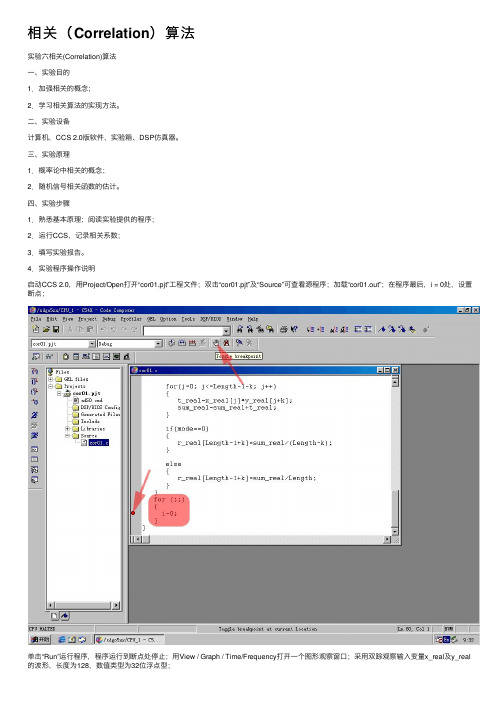
4.实验程序操作说明启动CCS 2.0,⽤Project/Open打开“cor01.pjt”⼯程⽂件;双击“cor01.pjt”及“Source”可查看源程序;加载“cor01.out”;在程序最后,i = 0处,设置断点;单击“Run”运⾏程序,程序运⾏到断点处停⽌;⽤View / Graph / Time/Frequency打开⼀个图形观察窗⼝;采⽤双踪观察输⼊变量x_real及y_real 的波形,长度为128,数值类型为32位浮点型;再打开⼀个图形观察窗⼝,以观察相关运算的结果;该观察窗⼝的参数设置为:变量为r_real,长度为255,数据类型为32位浮点数;调整观察窗⼝,观察两路输⼊信号相关运算的结果;程序中,mode可赋0或1,赋0时,完成相关函数⽆偏估计的计算,赋1时,完成相关函数有偏估计的计算;x_real和y_real为参与相关运算的两路信号,当x_real = y_real时,完成⾃相关函数的计算,⽽当x_real y_real时,完成互相关函数的计算。
修改以上参数,进⾏“Rebuild All”,并重新加载程序,运⾏程序可以得到不同的实验结果。
关闭“cor01.pjt”⼯程⽂件,关闭各窗⼝,实验结束。
五、思考题⽤其他数学⼯具计算相关系数,并与实验结果⽐较(如:SPSS,MA TLAB)。
六、相关算法时域表达式: ()()()∑--=+=lN ln n s l n s l R 121七、程序参数说明x_real[Length] // 原始输⼊数据A y_real[Length] // 原始输⼊数据B r_real[Lengthcor] // 相关估计数值Length // 输⼊数据长度 Lengthcor // 相关计算结果长度 mode = 0 // ⽆偏估计 mode = 1 // 有偏估计⼋、程序流程图:实验七 u_LAW 算法⼀、实验⽬的1.学习u-律的基本原理、压扩特性、编码和解码⽅法; 2.学习u-律算法在DSP 上的实现⽅法。
- 1、下载文档前请自行甄别文档内容的完整性,平台不提供额外的编辑、内容补充、找答案等附加服务。
- 2、"仅部分预览"的文档,不可在线预览部分如存在完整性等问题,可反馈申请退款(可完整预览的文档不适用该条件!)。
- 3、如文档侵犯您的权益,请联系客服反馈,我们会尽快为您处理(人工客服工作时间:9:00-18:30)。
a rXiv:as tr o-ph/963112v12Mar1996Correlation Between BATSE Hard X-ray Spectral and Timing Properties of Cygnus X-1D.J.Crary 1,C.Kouveliotou 2,J.van Paradijs 3,4,F.van der Hooft 4,D.M.Scott 2,W.S.Paciesas 3,M.van der Klis 4,M.H.Finger 2,B.A.Harmon 5,and W.H.G.Lewin 6Received 1995December 18;accepted 1996March 1ABSTRACTWe have analyzed approximately1100days of Cygnus X-1hard X-ray data obtained with BATSE to study its rapid variability.Wefind for thefirst time correlations between the slope of the spectrum and the hard X-ray intensity,and between the spectral slope and the amplitude of the rapid variations of the hard X-rayflux.We compare our results with expectations from current theories of accretion onto black holes.Subject headings:X-rays:stars—stars:individual(Cygnus X-1)1.IntroductionAccreting black-hole candidates(BHC)in X-ray binaries show three‘source states’that are distinguished by characteristic spectral and(correlated)fast-variability properties. They are called the‘low state’,‘high state’and‘very high state’;the dominant parameter that determines the source state is likely to be the mass accretion rate(see Van der Klis 1995b,and Tanaka&Lewin1995for recent reviews).In the low state the X-ray spectrum is dominated by a very hard power law component extending to several hundreds of keV.The source intensity shows strongfluctuations,with broad-band r.m.s.amplitudes as high as40percent.At frequencies above∼1Hz the power density spectrum(PDS)of these variations follows a power law;at frequencies below a low-frequency cut offthe PDS isflat.In several BHC the cut-offfrequencyνc has been observed to vary by up to an order of magnitude,while the high-frequency part of the PDS remained approximately constant(Belloni&Hasinger1990;Miyamoto et al.1992).As a result,the power integrated over a frequency range belowνc is strongly anti-correlated with that cut-offfrequency.In the high state the X-ray spectrum contains an ultra-soft thermal component,with (bremsstrahlung)temperatures of order1keV.In some sources(e.g.,LMC X-3,see Tanaka 1989)the power-law spectral component is not detected,but in others(e.g.,GS1124−68, see Ebisawa et al.1994)it is observed in combination with the ultra-soft component.In the1–10keV range the amplitude of the intensity variations is correlated with photon energy;this can be understood if the variability is connected with the power law spectral component,which is‘diluted’by the much lower variability of the ultrasoft emission(Van der Klis1994).In the very high state the PDS of BHC show3–10Hz quasi-periodic oscillations and branch structure in an X-ray color-color diagram reminiscent of the normal-branch(NB)state of Z sources(Van der Klis1995a),i.e.,accreting neutron stars with magneticfields of order1010G.In view of the strong arguments that the accretion rate of Z sources is then close to the Eddington limit it has been suggested that in the very high state the BHC are likewise accreting near the Eddington limit(Van der Klis1995b).In their low state the BHC are remarkably similar to atoll sources,i.e.,accreting neutron stars with magneticfield strengths generally believed to be below109G(substantially weaker than those of Z sources).At low accretion rates,i.e.,in their so-called‘island state’, atoll sources have power law X-ray spectra(see,e.g.,Barret&Vedrenne1994).On average, these spectra appear to be not quite as hard as those of low-state BHC(see,e.g.,Gilfanov et al.1995);however,the distribution of the spectral slopes of BHC and atoll sources shows clear overlap(Wilson et al.1995;Ebisawa et al.1994;see also Van Paradijs&Van der Klis1994).Also,the PDS of island-state atoll sources are very similar to those of low-state BHC.They follow a power law at high frequencies,and areflat below a cut-offfrequency; the high-frequency part of the PDS of the atoll source1608−522was observed to remain approximately constant as the cut-offfrequency varied,like for Cyg X-1(Yoshida et al. 1993).As part of our attempt to gain a better understanding of the similarities between accreting BHC and neutron stars we are studying the variability of bright BHC using the almost continuous record provided by the Burst and Transient Source Experiment (BATSE)on the Compton Gamma Ray Observatory.We here report on a variability record of Cyg X-1,covering approximately1100days,and we show that the amplitude of its variations are strongly correlated with the slope of the hard X-ray spectrum,and that correlations exist between the amplitude of the variations and the totalflux.2.Data AnalysisTo quantify the rapid variability,we have created PDS from the1.024second time resolution large area detector(LAD)count rate data,(the so-called DISCLA data)using two energy channels covering the range20–50and50–100keV.These data werefiltered to eliminate bursts,Earth magnetospheric events,etc.,then searched for data segments of 512contiguous time bins(524.288seconds without gaps)when the source was above the Earth’s limb.During outburst of the bright transients GRO J0422+32and GRO J1719−24 the data from detectors that had these sources in theirfields of view were eliminated from consideration.On average,we selected40intervals of these512-bin data strings per day, amounting to a total data set of2.2×107seconds.The data for each detector and each energy channel were individuallyfit to a quadratic polynomial and thefit residuals converted to Fourier amplitudes using standard fast Fourier transform ing similar524.288second intervals obtained when the source was occulted by the Earth,we have determined that the quadratic detrending of the raw data yields a background(source occulted)power level that isflat between0.01Hz and the Nyquist frequency(0.488Hz).The power level in these background data is very close to Poissonian;using the normalization of Leahy et al.(1983),in which Poisson noise corresponds to a power density2.0,the background power density level equals2.040±0.005. This latter value has been subtracted from the data,so that these corrected data reflects the contribution to the PDS from Cyg X-1only.Deadtime corrections are not important for the count rate data used here.The Fourier transforms of each data segment were then summed coherently and converted to PDS.We made daily averages of these PDS over all segments selected for that day.After subtraction of the average background noise level these were normalized to the squared fractional r.m.s.amplitude per unit frequency(Van der Klis1995b)using the dailyaveraged detector count rates in the20–100keV energy band obtained from the BATSE occultation analysis(Harmon et al.1993).As a measure of the variability of the hard X-ray flux of Cyg X-1we used the fractional r.m.s.amplitude,f,of the intensityfluctuations in the frequency range0.03–0.488Hz,obtained by integrating the power spectral density(Van der Klis1995b).3.ResultsFrom their investigation of the1–25keV variability of Cyg X-1Belloni and Hasinger (1990)found that the cut-offfrequencyνc in the PDS varies between0.01and0.1Hz;since the high-frequency part of the PDS remains constant,the cut-offfrequency is anti-correlated with the power level at,and below,that frequency.Crary et al.(1996a)have confirmed this result for the20–100keV range using the data discussed here.We have searched for a possible correlation of the variability of Cyg X-1,and its hard X-ray intensity and spectral shape.The latter quantities were obtained from the 45–140keV X-ray light curve of Cyg X-1,which has been monitored with BATSE since the beginning of the CGRO mission(Paciesas et al.1996).The45–140keVflux,F,is generally between0.07and0.15cm−2sec−1,with no prominent long term(>50day)trends in the data evident through most of this period.At about Truncated Julian Day(TJD =JD−2440000.5)9250(1993September20),the sourceflux gradually declined over a period of about150days to a level of∼0.01cm−2sec−1.After that,theflux rose within30 days,back to a level of approximately0.1cm−2sec−1.Although it is not possible,on the basis of BATSE observations alone,to determine the source state of Cyg X-1during these observations,the presence of a hard component in the BATSE energy range indicates that Cyg X-1was probably in the low state during most of the BATSE observations;during the low-flux episode between TJD9250and9430a temporary transition to the high state mayhave occurred.In Figure1we show a plot of f versus F.In the following discussion we will distinguish the data from the low-flux episode(indicated by squares in Fig.1)from the remainder of the data(indicated by asterisks).We have included only days when F was higher than0.04 cm−2sec−1;below thisflux,f is dominated by detector noise due to unresolved sourcesin the uncollimated LADfield of view(Crary et al.1996b),and the measured value of f becomes uncertain.Typical errors are shown,calculated from the variance per bin of the daily averaged power spectra propagated through the calculation of f,and from the results of the occultation analysis averaged over an entire day.From Figure1it appears that during the low-flux episode(TJD9250–9430),Cyg X-1 showed relatively little variability,with f generally below12%.These low-flux data by themselves do not show a correlation between f and F;similarly,the remaining points in Figure1,with f usually in the range10–30%,do not show such correlation either.However, all points together follow a broad,upturning band in Figure1,which indicates that there is a relation between the hard X-rayflux of Cyg X-1and its variability.If during the low-flux episode Cyg X-1was in the high state,this result would suggest a dependence of the hard X-ray variability on source state.Although previous observations of other black-hole candidates have indicated that theflux in the hard tail of the energy spectrum decreases as the source enters a high state(this,however,is very uncertain,see Gilfanov et al.1995,and Tanaka&Lewin1995),the hard X-rayflux alone may not be a good marker of source state.However,the lack of low energy(1–10keV)observations prevents us from drawing afirm conclusion on this.Note that the low value of f is not the result of dilution of the variability of a hard spectral component by a less variable soft component.In Figure2we have plotted f versus the exponent,α,of a power lawfit to the45–140keV spectrum(Paciesas et al.1996);thisfigure shows that these two quantities are strongly correlated.The data obtained during the low-flux episode are offset systematically from the other data,showing both a softer spectrum(by about0.4inα)and smaller variability. However,the correlation between f andαdoes not reflect this systematic offset:the same correlation is followed by each of the two groups of points separately.The offset of the data from the low-flux episode from the other data,shown in both Figures1and2leads one to suspect that the hard X-rayflux and spectral slope of Cyg X-1 are also correlated.Figure3,which shows a plot ofαversus F,confirms this suspicion. Again,the two groups of data points are clearly separated in this diagram.However,for each of the two groups of points separately the correlation is not apparent(for the‘high-flux’points a correlation in the opposite sense may actually be present).4.ConclusionsWe have found a strong correlation between the slope of the high-energy(20-100keV) X-ray spectrum of Cyg X-1and both its high-energy X-rayflux and the variability thereof. During most of our observations Cyg X-1showed strong variability with an amplitude that varied in anti-correlation with a cut-offfrequency(Crary et al.1996a)similar to the low-state behavior in the lower-energy range described by Belloni and Hasinger(1990).It is therefore likely that we encountered Cyg X-1mainly in the low state.During a150day interval beginning in1993September both the high-energy X-rayflux and its variability were extremely low;it is possible that Cyg X-1had then entered a high state;this remains uncertain,due to lack of low-energy coverage.The global correlations we have found betweenflux,variability and spectral hardness suggest to us that all three are determined by a basic system parameter;the mass accretionrate is the obvious candidate.A variety of models have been calculated for the structure of the accretion disks around black holes,to explain the two-component character of their X-ray spectra,and the suspected relation of these spectral components with accretion rate (Liang&Nolan1984,and references therein;see also Haardt et al.1993;Chakrabarti& Titarchuk1995).Most of these models invoke a very hot medium,e.g.,a corona around the inner disk regions,that produces the hard power law component through upscattering of low-energy photons,and a standard Shakura-Sunyaev disk that provides the latter.Most of these models do not address source variability.The fast variability of Cyg X-1and other black holes has often been described in terms of shot noise models;the break frequency in the PDS reflects the decay time of the shots (Sutherland,Weisskopf,&Kahn1978;Miyamoto&Kitamoto1989;Belloni&Hasinger 1990).However,the X-ray spectral properties are usually not considered in these models.Mineshige et al.(1994,1995),proposed that accretion disks around black holes are in a self-organized critical state.Their qualitative arguments,aimed at an understanding of the low and high states,indicate that relatively hard X-ray spectra go with strong variability, and relatively soft X-ray spectra with weak variability.Chakrabarti&Titarchuk(1995)recently argued that accretion disks around black holes contain a shock,at several tens of Schwarzschild radii.In the low state,the post-shock region is quite hot,and the emergent spectrum is very hard(α<2.5).In this model,αincreases with disk accretion rate in the low state.Also in this context,Molteni,Sponholz, &Chakrabarti(1996)found that over a range in mass accretion rates the cooling time of theflow inside the shock is comparable to the infall time scale.Under these conditions the location of the shock,and the X-ray luminosity,undergoes quasi-periodic oscillations.The centroid frequency of these oscillations increases with the mass accretion rate,with typicalvalues around5Hz for a5M⊙black hole.This result may be related to the anti-correlation betweenαand f for Cyg X-1,by using the recent results of Van der Hooft et al.(1996)on the PDS of the black-hole transient GRO J1719−24.They found that the detailed shape of the PDS remained invariant under a frequency shift marked by the variation of a strong QPO peak(between∼40and∼300 mHz),while also the power in a given(stretched and squeezed)‘rest frequency’interval remained constant.This would suggest that the QPO frequency is proportional to a break frequency in the PDS of this source,and that the latter may be used as a frequency scaler as well.If we are allowed to generalize this result for GRO J1719−24to Cyg X-1,at least the direction of the correlation betweenαand f found by us for Cyg X-1would be accounted for by the model described by Chakrabarti&Titarchuk(1995)and Molteni et al.(1996).At super-Eddington disk accretion rates the model of Chakrabarti&Titarchuk(1995) predicts that theflow inside the shock is cooled by Comptonization of low energy photons from the disk,and the post-shockflow becomes predominantly radial(and converging). Comptonization in this region can still occur due to bulk motions,producing a hard tail withα∼2.5.The value ofαincreases weakly with the accretion rate;note however that in this model the X-ray luminosity may not be a good measure of the accretion rate as part of the internal energy in the disk is advected into the black hole(see also Narayan, McClintock,&Yi1996).In this regime theflux variability is determined by the variability of the illumination geometry of the converging inflow,and not by the change in the size of the post-shock region,as it is in the low state.The amplitude variation of the hardflux is expected to be smaller in this case(corresponding to the high state,since the increase in disk accretion rate leads to a increase in soft emission)than in the low state.It appears, then,that these theoretical results are in qualitative agreement with the data from thelow-flux episode that we have observed in Cyg X-1.The correlations we have found for Cyg X-1would easily have escaped attention were it not for the1100days of continuous coverage provided by the BATSE all-sky monitoring capabilities.We are looking forward to an improved understanding of our results in terms of the source state framework for black holes(Van der Klis1994)by combining the BATSE hard X-ray monitoring with that provided in the near future at low energies by XTE.We would like to thank the referee,Lev Titarchuk,for helpful comments.This project was performed within NASA grant NAG5-2560and supported in part by the Netherlands Organization for Scientific Research(NWO)under grant PGS78-277.This work was performed while DJC held a National Research Council-NASA Research Associateship.FvdH acknowledges support by the Netherlands Foundation for Research in Astronomy withfinancial aid from NWO under contract number782-376-011,and the Leids Kerkhoven–Bosscha Fonds for a travel grant.JvP acknowledges support from NASA grant NAG5-2755.WHGL acknowledges support from NASA grant NAG8-216.REFERENCESBarret,D.,&Vedrenne,G.1994,ApJS,92,505Belloni,T.,&Hasinger,G.1990,A&A,227,L33Chakrabarti,S.K.,&Titarchuk,L.G.1995,ApJ,455,623Crary,D.J.,et al.1996a,A&AS,submittedCrary,D.J.,et al.1996b,ApJ,in pressEbisawa,K.,et al.1994,PASJ,46,375Gilfanov,M.,et al.1995,in The Lives of the Neutron Stars,eds.M.A.Alpar,¨U.Kiziloˇg lu, &J.van Paradijs(Dordrecht:Kluwer Academic Publishers),331Haardt,F.,Done,C.,Matt,G.,&Fabian,A.C.1993,ApJ,411,L95Harmon,B.A.,et al.1993,AIP Conf.Proc.280,First Compton Gamma Ray Observatory Symposium,ed.M.Friedlander,N.Gehrels,&D.J.Macomb(New York:AIP),313 Leahy,D.A.,Darbro,W.,Elsner,R.F.,Weisskopf,M.C.,Sutherland,P.G.,Kahn,S.,& Grindlay,J.E.1983,ApJ,226,160Liang,E.P.,&Nolan,P.L.1984,Space Sci.Rev.,38,353Mineshige,S.,Takeuchi,M.,&Nishimori,H.1994,ApJ,435,L125Mineshige,S.,Kusnose,M.,&Matsumoto,R.1995,ApJ,445,L43Miyamoto,S.,&Kitamoto,S.1989,Nature,342,774Miyamoto,S.,Kitamoto,K.,Iga,S.,Negoro,H.,&Terada,K.1992ApJ,391,L21 Molteni,D.,Sponholz,H.,&Chakrabarti,S.K.1996,ApJ,457,805Narayan,R.,McClintock,J.,&Yi,I.1996,ApJ,457,821Paciesas,W.S.,et al.1996,ApJ,in preparationSutherland,P.G.,Weisskopf,M.C.,&Kahn,S.M.1978ApJ,219,1029Tanaka,Y.1989,in Proc.23rd ESLAB Symposium on Two Topics in X-ray Astronomy,ed.J.Hunt&B.Battrick(Paris:ESA Publications Division),p.3Tanaka,Y.,&Lewin,W.H.G.1995,in X-ray Binaries,ed.W.H.G.Lewin,J.van Paradijs,&E.P.J.van den Heuvel(London:Cambridge University Press),126Van der Hooft,F.,et al.1996,ApJ,458,L75Van der Klis,M.1994,ApJS,92,511Van der Klis,M.,1995a,in The Lives of the Neutron Stars,eds.M.A.Alpar,¨U.Kiziloˇg lu, &J.van Paradijs(Dordrecht:Kluwer Academic Publishers),301Van der Klis,M.1995b,in X-ray Binaries,W.H.G.Lewin,J.van Paradijs,&E.P.J.van den Heuvel(London:Cambridge University Press),p.252Van Paradijs,J.&Van der Klis,M.1994,A&A,281,L17Wilson,C.A.,Harmon,B.A.,Zhang,S.N.,Paciesas,W.S.,&Fishman,G.J.1995,IAU Circ.6152Yoshida,K.,Mitsuda,K.,Ebisawa,K.,Ueda,Y.,Fujimoto,R.,Yaqoob,T.,Done,C.1993, PASJ,45,605Fig.1–Cyg X-1fractional r.m.s.amplitude(0.03–0.488Hz)in the20–100keV band versus 45–140keVflux(cm−2sec−1).Fig.2–Fractional r.m.s.amplitude(0.03–0.488Hz)in the20–100keV band versus photon power law index from afit in the45–140keV range.Fig.3–Cyg X-145–140keVflux versus photon power law index from afit in the45–140 keV range.Fig.1.—Fig.2.—Fig.3.—。