CSDMS TauDEM Exercise
姜黄素在神经系统疾病治疗中的应用
姜黄素在神经系统疾病治疗中的应用
陈思砚
【期刊名称】《上海交通大学学报(医学版)》
【年(卷),期】2010(030)006
【摘要】姜黄素是一种天然多酚.近年来,姜黄素的抗炎症、抗氧化、免疫调节、促凋亡等药理作用已在神经系统疾病的研究中得到证实,特别是在基因及信号通路转导多重水平中的作用,已经成为研究热点.文章就姜黄素的生物学特性及其在神经系统疾病中的研究进展作一综述.
【总页数】4页(P732-734,741)
【作者】陈思砚
【作者单位】上海交通大学,医学院瑞金医院神经科神经病学研究所,上海,200025【正文语种】中文
【中图分类】R915;R741.05
【相关文献】
1.艾地苯醌在神经系统疾病治疗中的应用 [J], 兰晓艳; 温德树; 马莉琴; 吴志武; 谢姚屹; 丘宇; 黄妍菊; 宋玲玲
2.尼古丁药理学作用机制及在神经系统疾病治疗中的应用研究进展 [J], 陆凡晟;徐晓铭;司成;张洋;戴建国
3.姜黄素及其纳米制剂在中枢神经系统疾病治疗中的应用 [J], 许洁;蒋岩;张欣欣;赵丽艳;张万明
4.姜黄素及其纳米制剂在中枢神经系统疾病治疗中的应用 [J], 许洁;蒋岩;张欣欣;
赵丽艳;张万明
5.光遗传学在中枢神经系统疾病治疗中的应用 [J], 班德翔;向振洋;刘洋;曹富江因版权原因,仅展示原文概要,查看原文内容请购买。
半胱亚磺酸脱羧酶(CSD)在成年小鼠生殖系统的表达及相关功能的研究

研
究
生: 范 晶 晶
指 导 教 师: 崔 胜
申 请 学 位 类 别: 理学博士
教授
专 业 领 域 名 称: 生理学
研 究 方 向: 动物生殖与发育调控
所 在 学 院: 生物学院
2009 年 5 月
博士学位论文
半胱亚磺酸脱羧酶(CSD)在成年小鼠生殖系 统的表达及相关功能的研究
范晶晶
指 导 教 师: 崔 胜 教授 申请学位级别:理学博士 论文提交日期:2009 年 4 月 论文答辩日期:2009 年 5 月 27 日 学位授予单位:中国农业大学 学位授予时间:2009 年 9 月 学 科 门 类: 生理学
2.免疫组织化学染色显示 CSD 在小鼠围着床期子宫中呈动态分布:妊娠 D1 和 D2 只定位 在子宫腔上皮细胞和腺上皮细胞中;D3 开始,大量基质细胞也表现出较强的 CSD 阳性着色,但 着床点周围的蜕膜细胞中无阳性反应;从 D9 开始,子宫 CSD 阳性反应明显减弱,D9 着床点之 间的子宫腔上皮和腺上皮细胞也表达 CSD;从囊胚到 D9 的胚胎都可检测到 CSD 阳性。高效液 相色谱(HPLC)测定结果显示,牛磺酸在子宫组织中的含量在胚胎发育早期和着床过程最高, 妊娠中期开始下降,后期最低,分娩以后又回升。CSD mRNA、蛋白在子宫表达变化与牛磺酸含 量变化的论文是我个人在导师指导下进行的研究工作及取得的研究成 果。尽我所知,除了文中特别加以标注和致谢的地方外,论文中不包含其他人已经发 表或撰写过的研究成果,也不包含为获得中国农业大学或其它教育机构的学位或证书 而使用过的材料。与我一同工作的同志对本研究所做的任何贡献均已在论文中作了明 确的说明并表示了谢意。
大麻二酚干预下力竭运动大鼠骨骼肌炎症相关基因的挖掘与验证
大麻二酚干预下力竭运动大鼠骨骼肌炎症相关基因的挖掘与验证1. 内容概要本研究旨在探索大麻二酚(CBD)在大鼠力竭运动后对骨骼肌炎症相关基因的影响,并对其进行验证。
通过力竭运动训练大鼠模型,模拟运动员在剧烈运动后的生理状态。
采用实时荧光定量PCR技术检测大鼠骨骼肌中炎症相关基因的表达水平。
给予大鼠不同剂量的CBD处理,再次检测炎症相关基因的表达变化。
通过Western blot和免疫组化方法验证CBD对炎症相关基因表达的影响。
本研究旨在为临床治疗运动员过度训练引起的骨骼肌损伤提供新的理论依据和实验基础。
1.1 研究背景随着现代社会节奏的加快,人们的生活压力逐渐增大,导致慢性疲劳综合征(CFS)等疾病的发病率逐年上升。
力竭运动是一种常见的诱发CFS的方法,而炎症在力竭运动大鼠中普遍存在。
探讨力竭运动大鼠骨骼肌炎症相关基因的变化,对于理解力竭运动诱发CFS的机制具有重要意义。
大麻二酚(CBD)作为一种具有抗炎、镇痛和神经保护作用的药物成分,近年来在医学领域引起了广泛关注。
CBD可以通过调节多种信号通路来减轻炎症反应。
本研究旨在利用CBD干预力竭运动大鼠,挖掘其骨骼肌炎症相关基因的变化,并验证这些变化与力竭运动诱导的炎症反应之间的关系,以期为进一步研究CFS的发病机制提供新的思路。
1.2 研究目的通过力竭运动刺激大鼠骨骼肌,模拟真实生活中的运动损伤情况,从而使骨骼肌处于炎症状态。
使用CBD干预大鼠骨骼肌炎症过程,观察其对骨骼肌炎症相关基因表达的影响。
通过挖掘与验证这些炎症相关基因,探讨CBD在骨骼肌炎症中的潜在作用机制。
1.3 研究意义本研究旨在探索大麻二酚(CBD)在大鼠力竭运动后对骨骼肌炎症相关基因表达的影响,以期为进一步理解和治疗相关疾病提供理论依据。
通过力竭运动刺激大鼠产生骨骼肌炎症反应,然后利用RNA干扰技术敲除炎症相关基因,再给予不同剂量的CBD处理,观察其对炎症相关基因表达水平的影响。
这将有助于揭示CBD在骨骼肌炎症过程中的作用机制,以及其可能的抗炎作用。
局部施用辣椒素可使Aδ纤维介导的激光诱发电位减小
局部施用辣椒素可使Aδ纤维介导的激光诱发电位减小佚名
【期刊名称】《中国疼痛医学杂志》
【年(卷),期】1996(000)003
【总页数】1页(P191)
【正文语种】中文
【相关文献】
1.皮层激光诱发电位研究证实:先激活C纤维能够抑制皮层对后来的Aδ传入的反应 [J], 刘瀛瀛(译);王锦琰(校)
2.辣椒素可使前列腺癌细胞自杀 [J], 施麒斓
3.低能量激光照射对脂多糖介导人牙周膜成纤维细胞炎性损伤的保护作用 [J], 靳晓兰;张亚男;孙成蕊;邹朝晖
4.TriQuint推出新氮化镓晶体管可使放大器尺寸减小50% [J],
5.Algenol微藻制乙醇工艺可使碳足迹减小67%~87% [J],
因版权原因,仅展示原文概要,查看原文内容请购买。
远志皂苷元调控tau蛋白磷酸化的实验研究
go r up r ie no m a a i . i s pe i e f a h o r e o e r m heh pp c m p we egv n r l s l ne T s ues cm nso c g up we er m v d fo t i o a e r us CA1
t fe to e he e c ft nuie n o e c ng s a d x o e ism e ha s . eh d i g ni n t ha e h n e plr t c nim M t o s S SD la ng l o a o y ce ni ab r t r
关键词 :tu蛋 白;磷酸化 ;远志 皂苷元 ;大鼠 a
D I 1 . 9 9 j i . 0 — 4 2 1 . 9 0 6 O : 0 3 6 / . n 1 5 5 0 . 0 2 O . 1 S s 0 3
中图分类号 :R 8 . 2 55
文献标 识码 :A
文 章编 号:10 —3 42 1 )90 4 —3 0 55 0 (0 20 —0 50
理。方法
清 洁级 s D雄性 大鼠 6 只 , 0 随机 分为对照组 、模型组 、多奈哌 齐组及远志 皂苷元低 、中、高剂量组, 每组
1 0只。侧脑 室注射寡 聚体形 式的 p淀粉样 蛋 白 ( p) 制备 A A D大 鼠模 型, 术后给 药组给予 不同剂量远志皂苷元和多
奈哌 齐灌 胃, 照组 和 A 型组 给予等量生理盐水灌 胃。应用免疫组 织化 学方法和蛋 白印迹 法检 测海 马 tu蛋 白激 对 D模 a 酶 (S一 GK 3 p、C K 5 和磷酸 酯酶 (P 1 P 2) D一) P - 、P 一 A 的表达水平 。结果 显升 高 ( P<0 0 ) . 1 。结论 与对 照组 比较 , 模型组 tu蛋 白激酶表 达明显升 a 高, 磷酸 酯酶表 达明显 降低 ( P<0 0) . 1 ;与模型组 比较, 远志皂苷元各剂量组蛋 白激酶表达 明显 降低, 酸酯酶表 达明 磷 远 志皂苷元能调 节 A D大鼠模型蛋 白激酶和磷 酸酯酶之 间的平衡 失调
西安大略和麦克马斯特大学骨关节炎指数用于膝退行性骨关节炎患者

西安大略和麦克马斯特大学骨关节炎指数用于膝退行性骨关节
炎患者
退行性骨关节炎(OSTEOARTHRITIS)是一种常见的慢性疾病,是因为关节软骨逐渐磨损而引起的疼痛、僵硬和关节失能。
随着人们生活水平的提高和老龄化人口的增长,在全球范围内,骨关节炎病例逐年增加。
因此,骨关节炎专家们研究开发了许多骨关节炎指数以帮助医生和患者诊断和治疗骨关节炎病例,其中西安大略和麦克马斯特大学骨关节炎指数是比较常用的两种。
西安大略骨关节炎指数(WOMAC)是由加拿大多个机构共同开发的一种系统评估方法。
该评估方法使用问卷,旨在评估患者膝关节疼痛、僵硬和功能障碍的程度。
WOMAC评分包括
三个方面:疼痛、身体功能和刚硬程度,其中每个方面包括不同的问题。
例如,在疼痛部分,问题包括在常规活动中是否感到膝关节疼痛,而在体能方面,问题包括有多少困难是走路时支持体重。
医生会根据病人的回答得出总分,以确定病人的病情程度和治疗效果。
相对于WOMAC,麦克马斯特大学骨关节炎指数(KOOS)更加广泛和全面。
它包括特定动态活动的问题,例如弯曲,步行和跳跃。
此外,它还评估了生活质量方面的问题,包括睡眠质量和情感状态。
因此,KOOS更适合对运动损伤引起的骨关节炎进行评估,而WOMAC更适合研究退行性骨关节炎的影响。
总的来说,西安大略和麦克马斯特大学骨关节炎指数是研究骨关节炎的重要工具。
通过使用这些评估工具,医生可以更好地
了解病情,在治疗过程中进行调整和跟踪治疗效果。
另外,患者也可以根据评估结果更好地了解他们的病情和治疗,从而更好地应对骨关节炎的挑战。
利用网络药理学和分子对接技术分析“猫爪草-_冬凌草”对肝癌的治疗作用机制
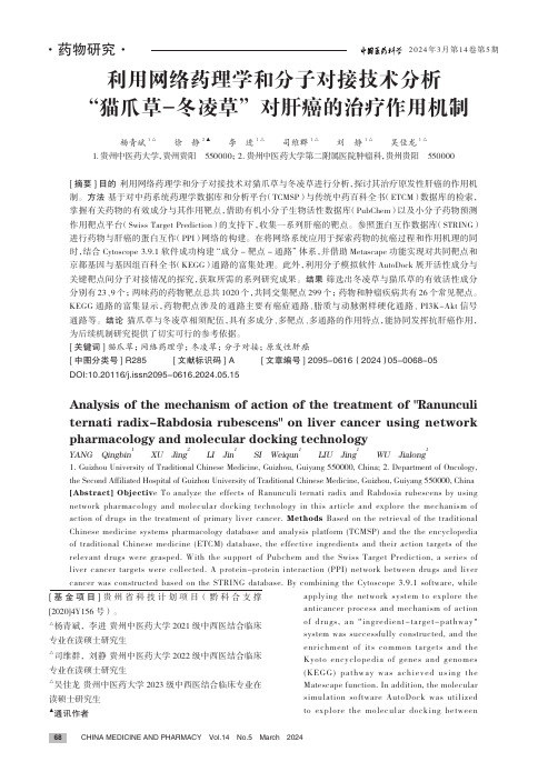
[基金项目]贵州省科技计划项目(黔科合支撑[2020]4Y156号)。
△杨青斌,李进 贵州中医药大学2021级中西医结合临床专业在读硕士研究生△司维群,刘静 贵州中医药大学2022级中西医结合临床专业在读硕士研究生△吴佳龙 贵州中医药大学2023级中西医结合临床专业在读硕士研究生▲通讯作者利用网络药理学和分子对接技术分析“猫爪草-冬凌草”对肝癌的治疗作用机制杨青斌1△ 徐 静2▲ 李 进1△ 司维群1△ 刘 静1△ 吴佳龙1△1.贵州中医药大学,贵州贵阳 550000;2.贵州中医药大学第二附属医院肿瘤科,贵州贵阳 550000[摘要]目的 利用网络药理学和分子对接技术对猫爪草与冬凌草进行分析,探讨其治疗原发性肝癌的作用机制。
方法 基于对中药系统药理学数据库和分析平台(TCMSP)与传统中药百科全书(ETCM)数据库的检索,掌握有关药物的有效成分与其作用靶点,借助有机小分子生物活性数据库(PubChem)以及小分子药物预测作用靶点平台(Swiss Target Prediction)的支持下,收集一系列肝癌的靶点。
参照蛋白互作数据库(STRING)进行药物与肝癌的蛋白互作(PPI)网络的构建。
在将网络系统应用于探索药物的抗癌过程和作用机理的同时,结合Cytoscope3.9.1软件成功构建“成分-靶点-通路”体系,并借助Metascape 功能实现对共同靶点和京都基因与基因组百科全书(KEGG)通路的富集处理。
此外,利用分子模拟软件AutoDock 展开活性成分与关键靶点间分子对接情况的探究,获取所需的系列研究成果。
结果 筛选出冬凌草与猫爪草的有效活性成分分别有23、9个;两味药的药物靶点总共1020个,共同交集靶点299个;药物和肿瘤疾病共有26个常见靶点。
KEGG 通路的富集显示,药物靶点涉及的通路主要有癌症通路、脂质与动脉粥样硬化通路、PI3K-Akt 信号通路等。
结论 猫爪草与冬凌草相须配伍,具有多成分、多靶点、多通路的作用特点,能协同发挥抗肝癌作用,为后续机制研究提供了切实可行的参考依据。
欧洲药品局发布了新的基于干细胞药物的指南

欧洲药品局发布了新的基于干细胞药物的指南李晗(译)【期刊名称】《药品评价》【年(卷),期】2011(8)4【摘要】欧洲药品局发布了新的基于干细胞药物的指南。
该指南涵盖了用于药物的不同类型的干细胞,并且考虑了当开发包括干细胞或从干细胞发育来细胞的药物时需将制药公司考虑在内。
【总页数】1页(P28-28)【关键词】欧洲药品局;干细胞;药物;指南;制药公司;细胞发育;同类型【作者】李晗(译)【作者单位】北京大学医药管理国际研究中心【正文语种】中文【中图分类】R95【相关文献】1.欧洲药品管理局人用药品委员会治疗慢性便秘药物研发临床评价指南介绍 [J], 闫雨佳;胡思源;杨娜;晋黎2.药品分类管理:破局与新局——[新局]之药物登记:形式大于内容? [J], 刘昕3.国家医保局发布《2019年国家医保药品目录调整工作方案》/两项“标准”发布助药品信息化追溯体系落地/糖尿病治疗药物聚乙二醇洛塞那肽注射液获批上市[J],4.勇气号火星车成功完成原定使命将继续工作/俄将发射载人飞船送3名宇航员到国际空间站/法国航天局计划发射新一代微卫星/阿丽亚娜5型火箭将两颗通信卫星成功送入轨道/美科学家纳米研究获得突破图像分辨率达0.7埃/德专家模仿昆虫复眼发明超薄成像系统/日本发明消除抗癌剂副作用的新疗法/基因疗法为阿尔茨海默氏症患者带来希望/瑞典科学家表示对成年干细胞再造器官能力存疑/欧洲药品评价署起草焦虑症药物指南/日本将有更多OTC药解除管理/转基因细菌可帮助治疗癌症/日本发现与细胞核分裂相关的蛋白质/英科学家:发现掌握双语的人更聪 [J], 5.FDA和欧洲药品管理局授予TB治疗药物SQ109“罕用药物”身份 [J], 姚瑜因版权原因,仅展示原文概要,查看原文内容请购买。
- 1、下载文档前请自行甄别文档内容的完整性,平台不提供额外的编辑、内容补充、找答案等附加服务。
- 2、"仅部分预览"的文档,不可在线预览部分如存在完整性等问题,可反馈申请退款(可完整预览的文档不适用该条件!)。
- 3、如文档侵犯您的权益,请联系客服反馈,我们会尽快为您处理(人工客服工作时间:9:00-18:30)。
CSDMS TauDEM Clinic "Hands On" ExerciseDavid Tarboton, dtarb@Utah State UniversityGoalBe able to use TauDEM tools to derive hydrologically useful information from Digital Elevation Models (DEMs)PurposeThe purpose of this exercise is to introduceHydrologic Terrain Analysis usingTauDEMand to guide you through the steps of running some of the more important functions required to delineate a stream network. Comprehensive documentation on the use of each TauDEM function is given in the online help that is part of the program.TauDEM (Terrain Analysis Using Digital Elevation Models) is a set of Digital Elevation Model (DEM) tools for the extraction and analysis of hydrologic information from topography as represented by a DEM. This is software developed at Utah State University (USU) for hydrologic digital elevation model analysis and watershed delineation and may be obtained from /taudem/taudem5.0/.In this exercise, you will perform the following tasks:-Basic Grid Analysis using TauDEM functions, including.-Pit Remove-D8 Flow Directions-D8 Contributing Area-Grid Network-D-Infinity flow direction-D-infinity Contributing Area-Stream Network Analysis using TauDEM functions, including-Stream Definition by threshold-Move Outlets to Streams-Stream Reach and Watershed-Peuker Douglas-Peuker Douglas Stream Definition-Specialized Grid Analysis using TauDEM functions, including-Wetness index derived from slope to area ratio-D-Infinity Distance DownThe Logan River watershed is used as an example.Computer SetupTo complete this exercise, you will need to use the TauDEM 5.0 software as well as MPICH2 software from /research/projects/mpich2/.You will also need to use visualizationsoftware such as ArcGIS or R. Refer to CSDMS Workshop setup instructions at/taudem/taudem5.0/documentation.html for computer setup details. Basic Grid Analysis using TauDEM functionsIn this section we illustrate the TauDEMbasic grid analysis functions.1.Download the Logan River example data zip file from/taudem/taudem5.0/LoganDemo.zip. Extract all files from the zip file.Look at the data.This data was obtained originally from the National Elevation Dataset seamless data server. See appendix 1 for how to obtain US DEM data from the USGS seamless data server and project it to a spatial reference system for the area of interest. Projected data should be used when working with TauDEM because TauDEM uses grid dimensions (cell size) in its length and slope calculations and these will be incorrect if they are not consistent in E-W and N-S directions and in the same units as the vertical units of the DEM.ArcMAP. Add data and adjust the symbology.Rz=raster("logan.tif")plot(z)2.The first TauDEM function used is Pit Remove. Pits are grid cells surrounded by higher terrain thatdo not drain. Pit Remove creates a hydrologically correct DEM by raising the elevation of pits to the point where they overflow their confining pour point and can drain to the edge of the domain.ArcMap.Open (by double clicking on) the TauDEM Pit Remove Tool (in the Basic Grid Analysis set)Select logan.tif for the Input Elevation Grid. Note that the Output Pit Removed Elevation Grid name is automatically filled with loganfel.tif following the file naming convention. Select the Input Number of Processes (I used 8 for a dual quad core PC).The parallel approach used by TauDEM is illustrated below. The domain is subdivided into row oriented partitions that are each processed independently by separate processes. When the algorithms reach a point where they can proceed no further within the partitions there is a swap step that exchanges information along the boundaries. The algorithms then proceed working within the partitions using new boundary information. This process is iterated until completion. The strategies for sharing information across boundaries and iterating are specific to each algorithm.The number of processes does not have to be the same as the number of processors on your computer, although generally should be the same order of magnitude. The operating system (and MPICH2) takes care of time sharing between processes, so in cases where some processes are likely to be waiting for other processes to complete there may be a benefit in selecting more processes than physical processors on the computer. However then message passing across the borders is increased. For large datasets, some experimentation as to the number of processes that works best (fastest) is suggested.Click OK on the Pit Remove tool to run the Pit Remove function for the Logan River DEM. The output dialog reports run statistics that include timing, as well as any error or warning messages.R# Pitremovesystem("mpiexec -n 8 pitremove -z logan.tif -felloganfel.tif")fel=raster("loganfel.tif")plot(fel)Command LineOpen a command prompt. Select Start -> All Programs -> Accessories -> Command PromptIn the command prompt type the equivalent on your computer tocdC:\Users\dtarb\Scratch\DemoThis changes directory to the folder where you are workingType (or cut and paste from here) into the command promptmpiexec -n 8 pitremove -z logan.tif -felloganfel.tifNote. Command line commands, are exactly the same as the string argument in R system calls so are not repeated in what follows. You can learn more about running TauDEM from the command line at: /taudem/taudem5.0/TauDEM5LineGuide.pdf3.The next function to run is D8 Flow Direction. This takes as input the hydrologically correct elevationgrid and outputs D8 flow direction and slope for each grid cell.ArcMapThe resulting D8 flow direction grid (grid has suffix p) is illustrated. This is an encoding of the direction of steepest descent from each grid cell using the numbers 1 to 8 per the embedded help above. This is the simplest model of the direction water would flow over the terrain.R# D8 flow directionssystem("mpiexec -n 8 D8Flowdir -p loganp.tif -sd8 logansd8.tif -felloganfel.tif",show.output.on.console=F,invisible=F)p=raster("loganp.tif")plot(p)sd8=raster("logansd8.tif")plot(sd8)Note that on the R system calls there is the option to include "show.output.on.console=F", and "invisible=F" in the arguments. TauDEM functions write to stderr and stdout. This output gives progress information and an indication of how long each program may take. For long tasks it is helpful to see this to get a sense of progress and get reassurance that the program has not crashed. These arguments enable this, rather than this output being held by R for display only when the task completes. These arguments may be included in any R system call, although this was for expedience not done in many of the calls below.4.The next function to run is D8 Contributing Area. This counts the number of grid cells drainingthrough (out of) each grid cell based on D8 flow directions.ArcMapThere are options to specify outlets and an input weight grid that were not used here. These are detailed in the tool help and allow calculations to be restricted to the area upstream of designated outlets (specified as a shapefile) and to accumulate an input weight field, rather than just counting contributing area as a number of grid cells.There is also an option to check for edge contamination. Edge contamination is a problem that can occur in the calculation of contributing area when flow is inwards from the boundary of the terrain. The computer does not know what the inflowing contributing area at the edge is, so evaluates the contributing area that may be impacted by this unknown area as no data. The result is streaks that enter the domain along flow paths. This is a desired result as it guards against missing parts of thewatershed, but it can and should be turned off if the DEM has been clipped to a watershed boundary. Red has been used to display no data to illustrate edge contamination.A logarithmic scale is often best to render contributing area values as in the illustration below.R# Contributing areasystem("mpiexec -n 8 AreaD8 -p loganp.tif -ad8 loganad8.tif")ad8=raster("loganad8.tif")plot(log(ad8)) # Use log scale for plottingzoom(log(ad8))5.The Grid Network function outputs three grids: (1) the longest flow path along D8 flow directions toeach grid cell, (2) the total length of all flow paths that end at each grid cell, and (3) the grid network order. This is obtained by applying the Strahler stream ordering system to the network defined starting at each grid cell.ArcMapR# Grid Networksystem("mpiexec -n 8 Gridnet -p loganp.tif -gordlogangord.tif -plenloganplen.tif -tlenlogantlen.tif")gord=raster("logangord.tif")plot(gord)zoom(gord)Grid Network Order (file name suffix gord) output from Grid Network is illustrated:The functions above used the D8 flow model that represents flow from each grid cell to one neighbor. TauDEM also uses the D (D-Infinity) flow model that calculates the steepest outwards flow direction using triangular facets centered on each grid cell and apportions flow between neighboring grid cells based on flow direction angles.6.The D-InfinityFlow Direction function is the starting point for all D-Infinity work. It calculates the D-Infinity flow directions for use in other TauDEM functions requiring D-infinity flow direction input.ArcMapR# DInf flow directionssystem("mpiexec -n 8 DinfFlowdir -angloganang.tif -slploganslp.tif -felloganfel.tif",show.output.on.console=F,invisible=F)ang=raster("loganang.tif")plot(ang)slp=raster("loganslp.tif")plot(slp)D-Infinity flow directions are encoded as angles counter clockwise from East in Radians as illustrated in the help.D-Infinity flow directions render similar to a hillshading.7.TheD-InfinityContributing Area function evaluates contributing area using the D-Infinity modelbased on flow being shared between grid cells proportional to the angle to the steepest downslope direction. This is designed to represent specific catchment area within dispersed flow over a smooth topographic surface.ArcMapR# Grid Networksystem("mpiexec -n 8 AreaDinf -angloganang.tif -scalogansca.tif")sca=raster("logansca.tif")plot(log(sca))zoom(log(sca))The result from running this is specific catchment area obtained from the D-Infinity contributing area function (with edge contamination) as illustrated below.Stream Network Analysis using TauDEM functionsTauDEM provides a number of methods for delineating and analyzing stream networks and watersheds. The simplest stream network delineation method uses a threshold on contributing area.8.Stream Definition by Threshold. This function defines a stream raster grid (src suffix) by applying athreshold to the input. In this case the input is a D8 contributing area grid and a threshold of 100 grid cells has been used.ArcMapR# Thresholdsystem("mpiexec -n 8 Threshold -ssa loganad8.tif -srclogansrc.tif -thresh 100") src=raster("logansrc.tif")plot(src)zoom(src)The result depicts the stream network as a binary grid (but is not logically connected as a network shapefile yet).9.Identify a watershed outlet. It is common to want to delineate watersheds upstream of an outlet,say a USGS stream gauge. This requires that gauge locations be precisely located on streams as rendered from the DEM. Due to inaccuracies in gauge locations and DEM stream delineation it is common for gauge locations not to be precisely on streams delineated from the DEM. The move Outlets to streams function slides gauge locations downslope following D8 flow directions until a stream (as defined by a stream raster grid) is encountered. An outlet shapefile can be created by clicking on or near a stream. I did this using the R function below.R# a quick R function to write a shapefilemakeshape.r=function(sname="shape",n=1){xy=locator(n=n)points(xy)#Pointdd<- data.frame(Id=1:n,X=xy$x,Y=xy$y)ddTable<- data.frame(Id=c(1),Name=paste("Outlet",1:n,sep="")) ddShapefile<- convert.to.shapefile(dd, ddTable, "Id", 1) write.shapefile(ddShapefile, sname, arcgis=T) }makeshape.r("ApproxOutlets ")This can also be done in ArcGIS using standard shape editing functionality.4340004360004380004400004420004440004618000462000046220004624000462600046280000.00.20.40.60.81.0ArcMapAdd the ApproxOutlets.shp file to ArcMap and zoom in to the area around it. Change the symbology if necessary.10.The Move Outlets to Streams function is used to move the outlets to the streams.ArcMapR# Move Outletssystem("mpiexec -n 8 moveoutletstostreams -p loganp.tif -srclogansrc.tif -o approxoutlets.shp -omOutlet.shp")outpt=read.shp("outlet.shp")plot(src)points(outpt$shp[2],outpt$shp[3],pch=19,col=2)Visualize the outlet.shp shapefile. Notice (below) how the outlet has been moved to coincide with the stream.It is somewhat overkill to use 8 processors to move one outlet point, but this is illustrative of how this could be used for many more points. Upon adding the moved outlet you may have received an ArcMAP unknown spatial reference warning. Be aware in using TauDEM that TauDEM does not do any spatial reference (projection) conversions. Therefore all data needs to be in the same spatial reference system. TauDEM does copy the spatial reference information from input grids to output grids, but does not do this for shapefiles.With the outlet positioned on the stream the stream network upstream of the outlet can be delineated.11.Once the outlet has been placed exactly on the stream paths, the D8 Contributing Area function isrun again, but specifying an outlet shapefile to evaluate contributing area and effectively identify the watershed upstream of the outlet point (or points for multiple outlets).ArcMapR# Contributing area upstream of outletsystem("mpiexec -n 8 Aread8 -p loganp.tif -o Outlet.shp -ad8 loganssa.tif") ssa=raster("loganssa.tif")plot(ssa)The result is contributing area only for the watershed upstream of the outlet.12.The next step is to use the Stream Definition By Threshold function to define streams using aspecified contributing area threshold. Here a threshold of 2000 grid cells is arbitrarily chosen ArcMapR# Thresholdsystem("mpiexec -n 8 threshold -ssaloganssa.tif -src logansrc1.tif -thresh 2000") src1=raster("logansrc1.tif")plot(src1)zoom(src1)The result is a grid stream network upstream of the outlet13.This network is still only represented as a grid. To convert this into vector elements representedusing a shapefile, the Stream Reach and Watershed function is used.ArcMapR# Stream Reach and Watershedsystem("mpiexec -n 8 Streamnet -felloganfel.tif -p loganp.tif -ad8 loganad8.tif -src logansrc1.tif -o outlet.shp -ordloganord.tif -tree logantree.txt -coord logancoord.txt -net logannet.shp -w loganw.tif")plot(raster("loganord.tif"))zoom(raster("loganord.tif"))plot(raster("loganw.tif"))# Plot streams using stream order as widthsnet=read.shapefile("logannet")ns=length(snet$shp$shp)for(i in 1:ns){lines(snet$shp$shp[[i]]$points,lwd=snet$dbf$dbf$Order[i])}The result is a number of outputs that need to be added to visualized. Here I visualized the watershed grid, loganw.tif, and stream network shapefile, logannet.shp, in R.The subwatershed raster and stream network shapefile are key outputs from TauDEM. Each link in the stream network has a unique identifier that is linked to downstream and upstream links. Each subwatershed also has a unique identifier that is referenced in terms of the stream network that it drains to. This information enables construction of a subwatershed based distributed hydrologic model with flow from subwatersheds being connected to, accumulated in, and routed along the appropriate stream reaches. It is interesting to zoom in on the outlet and examine the properties of the stream network and subwatersheds near the outlet to identify how the linkages between stream links are represented and what other attributes there are for each stream link. This is easiest to do in an interactive visualization system such as ArcMap. It is a little cumbersome in R.An important question in stream network delineation is what stream delineation threshold to use. The above used an arbitrary thresholds of 2000 grid cells. TauDEMalso provides ways to do select stream delineation threshold objectively using a stream drop test following theory described in Tarboton et al. (Tarboton et al., 1991; 1992) and Tarboton and Ames (2001). This may be combined with moregeomorphologically based methods for channel definition that attempt to capture topographic texture and spatial variability in drainage density. These will be illustrated next.14.The Peuker Douglas function produces a "valley" network skeleton following the proceduredescribed in their paper (Peuker and Douglas, 1975).ArcMapR# Peuker Douglas stream definitionsystem("mpiexec -n 8 PeukerDouglas -felloganfel.tif -ssloganss.tif")ss=raster("loganss.tif")plot(ss)zoom(ss)The result, derived entirely from a local filter applied to the topography is a skeleton of a stream network illustrated below15.The Peuker Douglas Stream Definition function has a rather extensive set of inputs. It configuresTauDEM to run Peuker Douglas, then use the Peuker Douglas stream skeleton as a weighted input toa D8 contributing area calculation. The result is then thresholded using a range of thresholds (thedrop analysis thresholds at the bottom of the input) to identify the smallest threshold for which the mean stream drop of first order streams is not significantly different from the mean stream drop of higher order streams. This is the constant drop law (Broscoe, 1959), and TauDEM uses it here to identify the highest resolution stream network that complies with this law as an objective way of identifying the stream delineation threshold.ArcMapThe output results include a table that reports the stream drop statistics for each threshold examined. This is included in the completion dialog as well as written to the drop analysis table file shown below. The last column of this gives T statistics for the differences of first and higher order streams. Using a threshold of |2| as indicating significance in this T test the threshold of 299 is chosen in this case as the objective stream delineation threshold.R. The ArcMap tool above ran 4 underlying TauDEM commands. The PeukerDouglas command was run earlier. Here are the next three.# Accumulating candidate stream source cellssystem("mpiexec -n 8 Aread8 -p loganp.tif -o outlet.shp -ad8 loganssa.tif -wgloganss.tif")ssa=raster("loganssa.tif")plot(ssa)# Drop Analysissystem("mpiexec -n 8 Dropanalysis -p loganp.tif -felloganfel.tif -ad8loganad8.tif -ssaloganssa.tif -drp logandrp.txt -o outlet.shp -par 5 500 10 0")# Deduce that the optimal threshold is 300# Stream raster by thresholdsystem("mpiexec -n 8 Threshold -ssaloganssa.tif -src logansrc2.tif -thresh 300") plot(raster("logansrc2.tif"))16.Next the Stream Reach and Watershed function is used to produce a vector stream shapefile fromthe resulting stream raster.ArcMapR# Stream networksystem("mpiexec -n 8 Streamnet -felloganfel.tif -p loganp.tif -ad8 loganad8.tif -src logansrc2.tif -ord loganord2.tif -tree logantree2.dat -coord logancoord2.dat -net logannet2.shp -w loganw2.tif -oOutlet.shp",show.output.on.console=F,invisible=F)plot(raster("loganw2.tif"))snet=read.shapefile("logannet2")ns=length(snet$shp$shp)for(i in 1:ns){lines(snet$shp$shp[[i]]$points,lwd=snet$dbf$dbf$Order[i])}Following is an illustration of the result. Notice how the stream network has been delineated more or less consistently with the contour crenulations depicting the texture of the topography.Specialized Grid Analysis using TauDEM functionsTauDEM also includes a number of specialized grid analysis functions. A few are illustrated here.17.The TOPMODEL wetness index is defined as ls(a/S) where a is specific catchment area and S is slope(tan of slope angle). In the TauDEM outputs above a is represented by sca, the D-Infinity specific catchment area grid and S by slp, the D-Infinity slope. sca is alreay in length units (the same units as grid cell size). TauDEM has a function to evaluate sar=S/a. This is done to leave to the user the choice as to how to handle grid cells that have S=0. Wetness index is then -ln(sar).ArcMapWetness index is evaluated using the ArcMap Raster CalculatorR# Wetness Indexsystem("mpiexec -n 8 SlopeAreaRatio -slploganslp.tif -scalogansca.tif -sarlogansar.tif", show.output.on.console=F, invisible=F)sar=raster("logansar.tif")wi=sarwi[,]=-log(sar[,])plot(wi)The result is illustrated below18.The D-Infinity Distance Down function computes the distance to streams (or any designated targetgrid) a number of different waysArcMapR# Distance Downsystem("mpiexec -n 8 DinfDistDown -angloganang.tif -felloganfel.tif -srclogansrc2.tif -m ave v -dd logandd.tif",show.output.on.console=F,invisible=F) plot(raster("logandd.tif"))By selecting-mave v as the distance method the result is the average vertical drop from each point, to a point on the stream as illustrated below.There are many other options for distance methods that are described in the help file/taudem/taudem5.0/TauDEM_Tools.chm and command line guide/taudem/taudem5.0/TauDEM5CommandLineGuide.pdf that you could experiment with if you want to.Appendix 1. Downloading DEM data from the USGS Seamless data server This appendix illustrates the process of downloading and projecting DEM data from the USGS Seamless data server, for the Cub River watershed as it drains to the location of a USGS streamflow station#10096000 located just north of Preston, Idaho, illustrated below.The USGS Seamless data server was used to obtain a National Elevation Dataset DEM.The steps followed were1.Access USGS Seamless data server /2.Click view and download United States Data3.Zoom to the area of interest. Activate layers on the right to help identify area of interest.4.Define a download region that covers the area of interest.5.Modify the data request to comprise the data sets (parameters) that you want to obtain6.Download the data. I selected the 1/3 arc second National elevation dataset DEM (≈ 10 m grid) Screen Image of the area that I selectedScreen Image of a Data Download RequestProjecting the Digital Elevation Model dataThe Digital Elevation Model grid from the Seamless Data Server is in Geographic Coordinates. Projected data should be used when working with TauDEM because TauDEM uses grid dimensions (cell size) in its length and slope calculations and these will be incorrect if they are not consistent in E-W and N-S directions and in the same units as the vertical units of the DEM. The DEM from the USGS was added to ArcMap. Then the ArcToolBox Project Raster tool was used to project this data. The ProjectRaster Tool is found within Data Management Tools / Projections and Transformations / Raster.In the Project Raster dialog that opens specify the input raster as the National Elevation Dataset DEM that was unzipped from the download. Name the output raster something convenient. Here I used "cubdem". Click on the button next to Output coordinate system to open the Spatial Reference Properties dialog.At this Spatial Reference Properties dialog click "Select" and navigate to the NAD_1927_UTM_Zone_12N projection being used as the standard spatial reference system for this exercise. Click OK.Back at the Project Raster dialog set the resampling technique to CUBIC (I have found by experience that this works best for DEMs) and set the output cell size to 20 m. The raw data in this case is at 1/3 arc second which is roughly 10 m. 20 m cell size is undersampling this a bit. Click OK. A processing dialog box should appear and after a few seconds indicate completion of the projection of the DEM. The DEM data has now been projected. The result is named 'cubdem'ReferencesBroscoe, A. J., (1959), "Quantitative analysis of longitudinal stream profiles of small watersheds," Office of Naval Research, Project NR 389-042, Technical Report No. 18, Department of Geology,Columbia University, New York.Peuker, T. K. and D. H. Douglas, (1975), "Detection of surface-specific points by local parallel processing of discrete terrain elevation data," Comput. Graphics Image Process., 4: 375-387.Tarboton, D. G. and D. P. Ames, (2001), "Advances in the mapping of flow networks from digital elevation data," World Water and Environmental Resources Congress, Orlando, Florida, May 20-24, ASCE, /dtarb/asce2001.pdf.Tarboton, D. G., R. L. Bras and I. Rodriguez-Iturbe, (1991), "On the Extraction of Channel Networks from Digital Elevation Data," Hydrologic Processes, 5(1): 81-100.Tarboton, D. G., R. L. Bras and I. Rodriguez-Iturbe, (1992), "A Physical Basis for Drainage Density,"Geomorphology, 5(1/2): 59-76.。
