18 A Novel Preprocessing Method Using Hilbert Huang Transform for MALDI-TOF and SELDI-TOF Mass Spect

合集下载

Improved prediction of signal peptides SignalP 3.0.

”J.Mol.Biol.,to appear2004.”Improved prediction of signal peptides—SignalP3.0 Jannick Dyrløv Bendtsen1,Henrik Nielsen1,Gunnar von Heijne3and Søren Brunak1∗1Center for Biological Sequence AnalysisBioCentrum-DTUBuilding208Technical University of DenmarkDK-2800Lyngby,Denmark3Stockholm Bioinformatics CenterDepartment of Biochemistry and BiophysicsStockholm UniversitySE-10691Stockholm,Sweden∗To whom correspondence should be addressed(email:brunak@cbs.dtu.dk) Keywords:Signal peptide,signal peptidase I,neural network,hidden Markov model, SignalPRunning title:Signal peptide prediction by SignalPWe describe improvements of the currently most popular method for predic-tion of classically secreted proteins,SignalP.SignalP consists of two diﬀerent predictors based on neural network and hidden Markov model algorithms, where both components have been updated.Motivated by the idea that the cleavage site position and the amino acid composition of the signal peptide are correlated,new features have been included as input to the neural network. This addition,combined with a thorough error-correction of a new data set, have improved the performance of the predictor signiﬁcantly over SignalP ver-sion2.In version3,correctness of the cleavage site predictions have increased notably for all three organism groups,eukaryotes,Gram-negative and Gram-positive bacteria.The accuracy of cleavage site prediction has increased in the range from6-17%over the previous version,whereas the signal peptide discrimination improvement is mainly due to the elimination of false positive predictions,as well as the introduction of a new discrimination score for the neural network.The new method has also been benchmarked against other available methods.Predictions can be made at the publicly available web server http://www.cbs.dtu.dk/services/SignalP/.1IntroductionNumerous attempts to predict the correct subcellular location of proteins using machine learning techniques have been developed1–putational methods for prediction of N-terminal signal peptides were published around20years ago,initially using a weight matrix approach1,2.Development of prediction methods shifted to machine learning al-gorithms in the mid1990’s10,11,with a signiﬁcant increase in performance12.SignalP,one of the currently most used methods,predicts the presence of signal peptidase I cleavage sites.For signal peptidase II cleavage sites found in lipo-proteins the LipoP predictor has been constructed13.SignalP produces both classiﬁcation and cleavage site assignment, while most of the other methods classiﬁes proteins as secretory or non-secretory.A consistent assessment of the predictive performance requires a reliable benchmark data set.This is particularly important in this area where the predictive performance is approaching the performance calculated from interpretation of experimental data,which is not always perfect.Incorrect annotation of signal peptide cleavage sites in the databases stems not only from trivial database errors,but also from peptide sequencing where it may be hard to control the level of post-processing of the protein by other peptidases, after the signal peptidase I has made its initial cleavage.Such post-processing typically leads to cleavage site assignments shifted downstream relative to the true signal peptidase I cleavage site.In the process of training the new version of SignalP we have generated a new,thor-oughly curated data set based on the extraction and redundancy reduction method pub-lished earlier14.Other methods were used for cleaning the new data set,and we found a surprisingly high error rate in Swiss-Prot,where,for example,in the order of7%of the Gram-positive entries had either wrong cleavage site position and/or wrong annotation of the experimental evidence.Also,we found many errors in a previously used bench-mark set12(stemming from automatic extraction from Swiss-Prot),and it appears that some programs are in fact better than the performance reported(predictions are correct, while feature annotation is incorrect).For comparison,we made use of this independent benchmark data set that was initially used for evaluation ofﬁve diﬀerent signal peptide predictors12.In the new version of SignalP we have introduced novel amino acid composition units as well as sequence position units in the neural network input layer in order to obtain better performance.Moreover,we have slightly changed the window sizes compared to the previous version.We have usedﬁvefold cross-validation tests for direct comparison to the previous version of SignalP10.In the previous version of SignalP a combination score,Y,was created from the cleavage site score,C,and the signal peptide score,S,and used to obtain a better prediction of the position of the cleavage site.In the new version, we also use the C-score to obtain a better discrimination between secreted and non-secreted sequences,and have constructed a new D-score for this classiﬁcation task.The architecture of the hidden Markov model SignalP has not changed,but the models have been retrained on the new data set,and have also signiﬁcantly increased their performance.2Results and discussionGeneration of data setsAs the predictive performance of the earlier SignalP method was quite high,assessment of potential improvements is critically dependent on the quality of the data annotation.We generated a new positive signal peptide data set from Swiss-Prot15release40.0,retaining the negative data set extracted from the previous work.The method for redundancy reduction was the same as in the previous work14,and was based on the reduction prin-ciple developed by Hobohm et al.16.Ourﬁnal positive signal peptide data sets contain 1192,334and153sequences for eukaryotes,Gram-negative and Gram-positive bacteria, respectively.In the previous work,we found many errors by detailed inspection of hard-to-learn examples during training and wrongly predicted examples.Nevertheless,we were quite sure that even after careful examination in this manner,the data set would probably still contain errors obtained from incorrect database annotation and wrongly interpreted laboratory results.Therefore,we developed a new feature based approach where abnormal examples can be detected by inspecting rare amino acid occurrences and outlier physical-chemical properties of signal peptides.In the following,we show that the isoelectric point of signal peptides can help inﬁnding possible annotation errors and other errors,where these errors may be due to the fact that some(long)signal peptides annotated in Swiss-Prot actually include probable propeptides.In such cases,convertase cleavage sites are mixed together with signal peptidase I cleavage sites.Removal of spurious cleavage site residuesExperimental assessment of the eﬀect of certain amino acids in the cleavage site region has shown that rare residues do not allow for eﬃcient cleavage17,18.Examination of amino acids around the signal peptidase I cleavage site in the data set revealed a number of sequences containing amino acids,which very rarely appear at the cleavage site.In the eukaryotic data set we found and removed seven sequences containing lysines (K)and13sequences containing arginines(R)at the−1position.All sequences with either a lysine or an arginine at position−1were investigated manually.All of them except one had a predicted cleavage site upstream of the annotated one.Most of these sequences probably undergo N-terminal maturation by diﬀerent proteases,either in the Trans Golgi Network(TGN)or after release from the cell as mentioned below in the section on propeptide analysis.In one clear case we found an obvious error in the Swiss-Prot entry NPAB LOCMI.According to the annotation the cleavage site is located between residues24-25(arginine in position−1),but in the original paper the authors identiﬁed the cleavage to occur between amino acids22-23.In this case,the two amino acids,ER, are removed by a dipeptidase19.Furthermore,we removed sequences where other amino acids appeared at position−1 in very few of the sequences.For the eukaryotic data set,the only allowed residues at position−1were alanine(A),cysteine(C),glycine(G),leucine(L),proline(P),glutamine (Q),serine(S)and threonine(T).By allowing only the latter amino acids we might have removed a few true,unusual sequences.For instance,tyrosine(Y)and histidine(H) at position−1were found only in one case each in the entire eukaryotic data set.We3removed eight sequences with aspartic acid(D)and eight with phenylalanine(F),seven each with glutamic acid(E)and asparagine(N),respectively.Five with methionine(M), three containing isoleucine(I)and two sequences containing tryptophan(W)at position −1were also removed.Some of these are in fact provable errors,in one of the aspartic acid examples,CLUS BOVIN20,the N-terminal peptide sequencing in the paper reports the cleavage as MKTLLLLMGLLLSWESGWA---ISDKELQEMST···,while Swiss-Prot annotates the sequence as being cleaved between D and K,thereby changing a common position−1 amino acid,alanine,into a rare one.Interestingly,SignalP predicts the cleavage site as reported in the paper.For Gram-positive and Gram-negative bacteria,only four residues were allowed at position−1.These residues were alanine(A),glycine(G),serine(S)and threonine (T)17,18.For the Gram-positive data set,this approach removed four sequences containing arginines(R),three containing valines(V),two containing lysines(K)and one sequence each of glutamic acid(E),leucine(L),asparagine(N),glutamine(Q),threonine(T)and tyrosine(Y).In the Gram-negative data set,we removed two sequences containing valine (V)at position−1and one sequence for each of the following amino acids,glutamic acid (E),lysine(K),leucine(L),asparagine(N),glutamine(Q).Isoelectric point calculationsPrevious studies have shown diﬀerences in amino acid composition between signal peptide and mature protein21,22.Thus,we examined to what extent the isoelectric point(pI)could be used as a unique feature of signal peptides.We calculated the pI for all signal peptides and the corresponding mature proteins in the data set and presented this in three scatter plots(Figure1).In the scatter plot for Gram-positive bacteria two very distinct clusters appear.Only three signal peptide outliers were found and by manual inspection of the corresponding Swiss-Prot entries,we found that these proteins most likely were either not carrying signal peptides,or were annotated wrongly.These outliers having pI values below8had the following Swiss-Prot ID’s CWLA BACSP, IAA2STRGS,COTT BACSU.The three entries have annotated signal peptides,but it is doubtful whether the annotation is correct.According to the prediction from SignalPprotein,indicated by s and m,respectively.Clusters of outlier examples for bacteria are indicated on the two plots.4and PSORT,CWLA BACSP does not carry a signal peptide.CWLA BACSP was in the paper described as a “putative”signal peptide 23and later it was indicated that cwlA is part of an ancestral prophage,still remnant in the Bacillus subtilis genome 24.All phage and virus sequences were initially removed from the SignalP training set,which could result in the negative prediction for this prophage sequence.The cleavage site in the alpha-amylase inhibitor IAA2STRGS turns out not to be ex-perimentally veriﬁed.It is predicted to have a cleavage site at position 26(SignalP)or 24(PSORT).Calculation of pI using the SignalP predicted signal peptide length gave a new result of 8.66,closer to the average for Gram-positive bacteria.The paper proposes two other cleavage site positions,but none of these have been veriﬁed experimentally 25.The last entry COTT BACSU is a spore coat protein from B.subtilis 26,27and no BLAST homologs in Swiss-Prot were found to contain an experimentally veriﬁed signal peptide.CotT is proteolytically processed from a 10kD precursor protein and is localized to spore coat where it controls the assembly.By N-terminal sequencing the N-terminus of the mature and processed protein was identiﬁed,although nowhere in the two papers is an SPase I cleavage site indicated,thus no signal peptide is mentioned 26,27.With the current knowledge about spore coats,spore coat assembly does not involve translocation of coat protein across any membrane 28–30.Hence,it is very unlikely for CotT to carry an N-terminal signal peptide as annotated in Swiss-Prot.The average isoelectric point of signal peptides and mature proteins in the entire Gram-positive data set was 10.59and 6.24,respectively.This is consistent with the fact that Gram-positive bacteria are known to have the longest signal peptides that carry more basic residues (K/R)in the n-region,than Gram-negatives and eukaryotes 11.When inspecting the scatter plot for Gram-negative bacteria,we ﬁnd the same overall clustering as observed for the Gram-positive bacteria,although not as distinct.Here the major group of signal peptides have pIs between 8and 13,although the variation is larger than in the Gram-positive scatter plot.A few sequence entries with acidic signal peptides were investigated in detail.Sequence entry SFMA ECOLI having a pI of 4.78was found to0.00.20.40.60.81.0010203040506070S c o r e Position SignalP-NN prediction (gram- networks): SFMA_ECOLI MES I NE I EG I YMKLRF I SSALAAALFAATGSYAAVVDG GT I HFEGELVNAACSVNTDSADQVVTLG QYRTC score S score Y scoreFigure 2:Alternative start codon assignment.The graphical output from SignalP strongly indicates erroneous annotation of the signal peptide from Swiss-Prot entry SFMA ECOLI .Further investigation showed a wrong annotation of the start codon (see text for details).C,S,and Y-score indicate cleavage site,“signal peptide-ness”and combined cleavage site predictions,respectively.5be an obvious erroneous annotation in Swiss-Prot.This entry had an annotated cleavage site at position22,but a predicted cleavage site at position34.As seen from Figure2we found an internal methionine at position12.Since the signal peptide-ness is very low until position12we assumed that this was an incorrectly annotated start codon.If the initial 11amino acids until the internal methionine were removed,SignalP correctly predicted the cleavage to be at position22and the pI of the signal peptide increased from4.78to 9.99.Indeed,in release41.0of Swiss-Prot this entry was corrected and the signal peptide marked“POTENTIAL”.For eukaryotes on the other hand,we were not able to distinguish the pI of the signal peptide and the mature protein.Eukaryotes have the shortest signal peptides and the amount of basic residues is much lower than for bacteria.Propeptide or signal peptide?For the eukaryotic data we examined whether annotated signal peptides could possi-bly include propeptides.In secreted proteins,propeptides are often found immediately downstream of the signal peptidase I cleavage site and their cleavage site is deﬁned by a conserved set of basic amino acids.Propeptides can be hard to detect by N-terminal Edmann degradation,as the propeptides are cleaved oﬀin the TGN before the release of the mature protein to the surroundings31.We used a new propeptide predictor,ProP,to predict propeptide cleavage sites32in the eukaryotic data set.In ten sequences we found a predicted cleavage site for a propeptide at the same position where a signal peptidase I cleavage site was annotated in Swiss-Prot. In all ten cases SignalP predicted a shorter signal peptide than annotated,thus making room for a short propeptide between the predicted signal peptide and the mature pro-tein.The ten sequences,AMYH SACFI,CRYP CRYPA,FINC RAT,GUX2TRIRE,LIGC TRAVE, MDLA PENCA,RNMG ASPRE,RNT1ASPOR,XYN2TRIRE,XYNA THELA,were reassigned accord-ing to the prediction of SignalP version2.0.This is an exceptional case where we tend to rate the computational analysis higher than experimental evidence,which must be considered weak,as the propeptide processing takes place before the proteins have been subjected to experimental,N-terminal peptide sequencing.After the signal peptide in these cases had been reassigned,we got marginally higher correlation coeﬃcients when retraining the neural network on the reassigned data set (data not shown).Optimization of window sizesAs in the earlier SignalP approach,the signal peptide discrimination and the signal peptidase I cleavage site prediction were handled using two diﬀerent types of neural networks10,33.We used a brute force approach to optimize the window sizes for the neural net-works by calculating single position correlation coeﬃcients for all possible combinations of symmetric and asymmetric ing this approach we trained approximately 6500neural networks for window optimization for a single organism group.This was furthermore done for diﬀerent combinations where amino acid composition and position information was included in the input to network or not,leading to approximately27000 neural networks being tested in all.6For eukaryotes,these data are shown in Figure 3.It is clear that optimal signal peptide discrimination prediction requires symmetric (or nearly symmetric)windows,whereas cleavage site training needs asymmetric windows with more positions upstream of the cleavage site included in the input to the network.The optimal window size for cleavage site prediction for the eukaryote network included 20positions upstream and 4positions downstream of the cleavage site.The window sizes for the Gram-positive networks were retained as previously found 10,whereas the Gram-negative cleavage site network included one more position downstream of the cleavage site,resulting in a window of 11positions upstream and 3positions downstream of the cleavage site.The eukaryote discrimination network performs best when using a symmetric window of 27positions.For both Gram-positive and Gram-negative bacteria the discrimination network is based on a symmetric window of 19positions.This brute force approach changed the optimal window sizes of the cleavage site network slightly from those used in SignalP 2.010,33.Network performanceWe have evaluated the performance of SignalP version 3.0using the same performance measures as used for the previous two versions of SignalP,see Table 1.The performance values were calculated using ﬁve fold cross-validation,i.e.testing on sequences not present in the training set (all data split into ﬁve subsets of approximately the same size).The most signiﬁcant performance increase was obtained for the cleavage site prediction as seen in Table 1.A performance increase of 6-17%for all three organism classes was obtained.We were able to optimize the signal peptide discrimination performance by introducing a new score,termed the D-score,replacing the earlier used mean S-score quantifying the “signal peptide-ness”of a given sequence segment.In the earlier versions of SignalP the scores from the two types of networks were combined for cleavage site assignment,and not for the task of discrimination.In the new version 3,the D-score is calculated as the average of the mean S-score and the maximal Y-score,and the two types of networks are 0.20.30.40.50.60.550.60.650.70.750.80.850.9Figure 3:Window optimization.These plots show single position level correlation coeﬃcients for all combinations of window sizes for the signal peptide cleavage and discrimination networks used for eu-karyotic signal peptide prediction.The optimal window size for cleavage site for the eukaryotic network included 20positions to the left and 4positions to the right of the cleavage site.For reasons of computa-tional eﬃciency we have selected a discrimination network with a symmetric window of 27amino acids,although networks with larger windows have slightly higher single position level correlation coeﬃcients.7then used for both purposes(see Material and Methods for details).Version Cleavage site(Y-score)Discrimination(SP/non-SP)Euk Gram−Gram+Euk Gram−Gram+ SignalP1NN70.279.367.90.970.880.96 SignalP2NN72.483.467.40.970.900.96 SignalP2HMM69.581.464.50.940.930.96 SignalP3NN79.092.585.00.980.950.98 SignalP3HMM75.790.281.60.940.940.98 Table1:Performances of three diﬀerent SignalP versions.The most signiﬁcant improvement was for the cleavage site predictions.Cleavage site performances are presented as%and discrimination values (based on D-score)as correlation coeﬃcients.NN and HMM indicate neural network and hidden Markov model,respectively.Results are based onﬁve-fold cross validation for all SignalP versions.Improvement by position information and composition featuresIn order to improve the performance of the neural network version of SignalP,we intro-duced two new features into the network input:information about the position of the sliding window as well as information on the amino acid composition of the entire se-quence.This information was encoded by additional input units in the neural network. The new position information units were found to be important for both the cleavage site and discrimination networks,whereas the amino acid composition information only improved the discrimination network.The idea of including compositional information is based on the observation that the composition of secreted and non-secreted proteins diﬀer21,22.The average length of signal peptides range from22(eukaryotes)and24(Gram-negatives)to32amino acids for Gram-positives,and the new network encoding the po-sition of the sliding window uses these averages to penalize prediction of extremely long or short signal peptides.Therefore,twin arginine signal peptides often receive a below threshold D-score as they tend to be quite long(average37amino acids)34,35.This also means that a few cases of ordinary signal peptides with extreme length are not predicted correctly by the neural networks.The HMM is also in its structure penalizing long signal peptides,and similarly the SignalP3HMM is not able to predict these cases correctly. One example36is the(NUC STAAU)with a63amino acid long signal peptide that is not pre-dicted correctly by any of the SignalP3models.SignalP3does not always fail to predict long signal peptides correctly,e.g.the56amino acids long signal peptide of CYGD BOVIN37 is handled correctly by the neural network version,both in terms of cleavage site and dis-crimination.However,great care should be taken when interpreting the scores for long potential signal peptides.From Figure4the importance of the new approach where position and amino acid composition information is included can be assessed.Including information of the position of the sliding window during training,increased the neural network cleavage site prediction performance slightly(left panel of theﬁgure).Composition information did not increase the performance of the cleavage site prediction,therefore it is excluded from the left panel in Figure4.But composition information did increase the performance of the discrimination network slightly(right panel of theﬁgure),whereas information of the8Figure4:Improvement of the neural network by introducing length and composition fea-tures.Position of the sliding window in the neural network input increased cleavage site prediction performance slightly(left panel).Amino acid composition information together with information of the position of the sliding window improved the discrimination network signiﬁcantly as seen in the right panel.The performance improvement was evaluated as single position level correlations during training on the individual networks for cleavage and discrimination,respectively.position of the sliding window together with composition increased the discrimination signiﬁcantly(right panel).Another improvement of the discrimination stems from the new D-score(see Table2).Theﬁnal prediction method uses both position and composition information.Eﬀect of the new discrimination scoreIn SignalP version3.0we have introduced a new discrimination score for the neural network,termed the D-score.Based on the mean S-score and maximal Y-score it was found to give increased discriminative performance over the mean S-score,used in SignalP version2.0.In Table2,the D-score shows superior performance over the mean S-score for the novel part of the benchmark set deﬁned by Menne et al.(see below).Dataset sensitivity speciﬁcity accuracy cc Gram−0.94(0.93)0.88(0.81)0.95(0.93)0.88(0.82) Gram+0.98(0.98)0.98(0.98)0.98(0.98)0.96(0.95)Table2:D-score outperforms the mean S-score for discrimination of signal peptide versus non-signal ing the novel part of the Menne test set12,we tested the D-score for discrimi-nation compared to the mean S-score.The mean S-score performances are shown in parentheses.The above mentioned56amino acid long signal peptide in CYGD BOVIN is an example where the D-score leads to a correct classiﬁcation,while the mean S-score is below the threshold.In this case the strong cleavage site score adds to a weaker signal peptide-ness in the C-terminal part of the leader sequence.Performance comparison to other prediction methodsAs described in a recent review of signal peptide prediction methods it is hard toﬁnd an ideal benchmark set,as methods have been frozen at diﬀerent times12.The data used to train a method is in general“easier”than genuine test sequences that are novel to a particular method.Since we have used a more recent version of Swiss-Prot than did9Menne et al.in their assessment,we have merely retained Menne set sequences that are not present in the SignalP version3.0training set.In this manner,we do not give an advantage to SignalP,as some of these sequences possibly have been included in the training set for other methods.We did not test the performance of the weight matrix-based methods SigCleave or SPScan as the earlier report shows that these are outperformed by machine learning methods12.SigCleave is based on von Heijne’s weight matrix2from1986.SPScan is also based on the weight matrix from von Heijne,but in addition to this it uses McGeoch’s criteria for a minimal,acceptable signal peptide1.We have tested other methods which are made available,one problem being that they do not necessarily predict the same organism classes,e.g.the PSORT-B method8does only predict on Gram-negative data,and not on the two other SignalP organism classes.The comparative results are given in Table3.For the PSORT-II method38,39which predicts on eukaryotic sequences,the subcellular localization classes“endoplasmic retic-ulum(ER)”,“extracellular”and“Golgi”were merged into one category of secretory proteins,whereas the rest“cytoplasmic”,“mitochondrial”,“nuclear”,‘peroxisomal”and “vacuolar”were merged into a single“non-secretory”category.The performance reported in the paper is57%correct for all categories.In Table3it can be seen that SignalP3 outperforms PSORT-II on this particular set with a signiﬁcant margin.PSORT-II does not assign cleavage sites,and we have therefore only compared the discrimination perfor-mance.We believe that the minor decrease in discrimination performance of SignalP3on this set,when compared to the cross-validation performance reported above in Table1,is a result of errors in the Menne set(originating from Swiss-Prot)together with its redun-dancy(see below),but more importantly,the presence of transmembrane helices within theﬁrst60amino acids in more than10%of the novel negative test sequences from this set(when analyzed by TMHMM40).The new version of PSORT(PSORT-B)has been trained onﬁve subcellular localiza-tion classes in Gram-negative bacteria and was reported to obtain a97%speciﬁcity and 75%sensitivity8.PSORT-B was optimized for speciﬁcity over sensitivity.Another recent method,SubLoc5predicts three subcellular compartments for prokaryotes and four com-Data set/Method sensitivity speciﬁcity accuracy cc Eukaryotes SignalP3-NN0.990.850.930.87 Eukaryotes PSORT-II0.650.750.800.56 Eukaryotes SubLoc0.580.700.770.47Gram−PSORT-B0.990.640.750.58 Gram−Subloc0.900.790.910.78 Gram+SignalP3-NN0.950.930.970.92 Gram+PSORT0.860.800.910.77 Gram+SubLoc0.820.920.860.76 Table3:Performance measures for signal peptide ing the novel part of the Menne et al.test set12we obtained the results shown in the table.Note that the values for PSORT-B is calculated on the part of the data set where PSORT-B produces a classiﬁcation.Around55%of the sequences were classiﬁed as“Unknown”,and the actual performance is therefore much lower than indicated here.For a given organism class the relevant version of PSORT has been used to make the predictions and calculated the performance.10。

蒸汽管线外表面传热系数计算模型修正

节能经济/Energy ConservationEconomy1现状新疆油田稠油产量占我国全年稠油总产量的1/3[1]，采集技术通常为热采技术，将蒸汽注入地下油层，以达到降黏增流、提高开采效率的目的[2]。

热采过程中，管道保温是实现稠油高效开采的基础[3]。

然而，受保温层结构偏心沉降等因素影响，蒸汽管线对流散热损失严重，蒸汽品质与能量利用率降低[4-5]，其中表面传热系数是计算蒸汽管线对流散热损失的重要参数[6-7]。

国内外学者对管线对流散热研究时，通常将管线外表面传热系数做相应的简化处理。

如李涛等人[8]分析了架空管道停输介质温度分布影响规律，发现表面传热系数增加，其管内介质温度低于凝固点所需的时间缩短。

另外，随着运行年份增加，管线保温结构因自重出现上薄下厚的偏心沉降，其结构非均匀分布会对外表面传热系数产生影响，如赵旭[9]采用努塞尔准则数获取管线外表面传热系数的方式进行了大截面热力管线保温层下沉的不等厚优化设计；Sahin等人[10-11]基于控制理论方法与梯度下降法研究了变保温厚度的铺设方案，但外表面传热系数是基于定值进行分析的。

上述研究侧重于将管线外表面传热系数简化为定值或无量纲准则数，但针对保温偏心沉降情况下的表面传热系数研究尚未见诸文献报道。

通过建立蒸汽管线保温结构变异二维稳态传热模型，分析保温结构偏心沉降程度对其表面传热系数的影响规律，从而获取保温管线不同分区部分的表面传热系数，并对现有经验关联式进行了修正，为油气田地面工程运维及相关规范修订提供参考。

2数理模型2.1架空蒸汽管线物理模型蒸汽管线物理模型见图1，模拟了其传热过程。

可见保温层结构因自重、阴雨天受潮等影响出现偏心沉降。

模型满足以下假设：管道壁面温度和室外空气温度保持不变；保温材料与管壁接触良好，忽略接触热阻的影响。

图1蒸汽管线物理模型管外空气流动状态：外表面温度与环境温度引发的空气密度差导致的自然对流，以及受风速影响引起的强制对流，需通过理查森数Ri判断二者作用规律。

A_Novel_Hierarchical_Structure_for_Multilayer_Perc

Theory and Practice of Science and Technology2022, VOL. 3, NO. 6, 4-10DOI: 10.47297/taposatWSP2633-456901.20220306A Novel Hierarchical Structure for Multilayer PerceptronGuodong Ma1, Zerui Qin21The Australian University, Canberra 2600,Australia2New York University,New YorkABSTRACTBased on the training set of the football game FIFA, the project developeda model that could classify the positions of players by their variousnumerical values. The model can select the best position for a player onthe field, providing strong guidance and suggestions for players toimprove the game experience. This problem is a multi-classificationproblem, the most important is to ensure the accuracy of modelclassification. We first try to use a classification model to classify the wholesample directly, and find that the accuracy is low. Then we introduced"hierarchical classification", that is to set up a hierarchical classificationmodel and realize the final classification step by step. We choose theneural network model as the classification model by comparing theaccuracy of four classification models. In the process of implementation,we also optimized the basic hierarchical classification model innovatively,which greatly improved its performance.KEYWORDSNeural Network; Multilayer Perceptron; Hierarchical Structure1　IntroductionThe project evaluates and classifies given players by collecting, processing, and analyzing various data (age, height, weight, physical, value, position, pace, shooting, dribbling, defending) of football players worldwide. Before, there have been researches on the position distribution of players, the selection of the top ten players, and overall prediction of a FIFA player. In real games, however, players are often placed in positions that do not fit their player stats. In this project, we train the player data of various league in the world, compare the efficiency of multiple classification models, and use the optimal model to achieve different degrees of position classification.2　DatasetThe project uses the FIFA complete player data sets in Kaggle[1] and FIFA's official website[2][3] to build the project model. The data sets contains 6 data sets provided the players data for career mode from FIFA 15 to FIFA 20. Each data set includes about 18,000 player information records of 104 aspects (e.g. id, name, various skill scores, etc.). This database has a lot of football analysis that can be studied and analyzed in depth by researchers. FIFA 20 data set is used as a training set to build a model, and FIFA 19 data set is used as a testing set to detect the model.Theory and Practice of Science and Technology 3　Solution(1)　Data set preprocessingThe project first deals with the wrong data (serial, missing, format error). The number of serial and format error samples in the data set is small, and these sample data are discarded from the data set. The project explores the reasons for the missing data.According to the Figure 1, The missing value is generated because the "goalkeeper" has no record meaning in some specific features; similarly, other players have no record meaning in the goalkeeper features. Therefore, there are no recorded values on these features. The project first excludes the "goalkeeper" samples in the data set, and then deleted the meaningless features from the remaining data set. The missing value is no longer included in the current data set.In order to better build the player position classification model, the project only retains 49 useful features, and the data type saved by all characters is changed to numeric form.The label of the data set originally has 11 categories. In order to better classify the label, the 11 categories are summarized into 4 categories and 9 categories, which are recorded in digital form (i.e. 0,1,2,3 and 0, 1...,8). Before implementing classification, the project explores the influence of the left and right feet on the position in advance. The project compared the ratio of the left and right feet to the left and right field positions (forward-field, mid-field, center-back-field, side-back-field). According to the Figure 2 , we can see that for the side-back-field players, the left-footed players are basically on the left field, and the right-footed players are basically on the right field. But for the midfield, backfield and center-side the use of the left and right feet of a player has little to do with being on the left and right side of the field. Therefore, in the classification process, we will finally further classify the side-back-field players (labeled L/RB) into two categories, LB and RB.(2)　Classification structure1)　Basic hierarchical classification structureAs shown in Figure 3, the algorithm first builds four classification models [4] for all players. Because the features of the players whose label is "GK" are different from those of the other three types of players, the algorithm first classifies the players with GK features into the goalkeeper category. Next, the algorithm builds a model to classify players into three categories by training set (2020 data set):"Forward", "Mid", and "Back".Figure 1　Missing value proportion 5Guodong Ma and Zerui Qin Through the classification model in the first step, four classifications will be obtained as a result. Next, the project further categorizes the "Forward", "Mid", and "Back" categories into 8 categories "ST", "R/LW", "CAM", "CDM", "CM", "R/LM" ,"CB", and "L/RB"[5]. The classification model in the second step is still built with the MLP model, and the test set is used to get the accuracy of the second-step classification (model1, model2, model3).Because we find that the left and right feet have a great influence on the left and right guards based on the preprocessing, the project finally divided the "L/RB" into two categories.The project compares 4 types of classification models (Logistic regression, decision tree [6], QDA, MLP [7]). Considering the efficiency and accuracy of the model, MLP is the optimal model. AndtheFigure 2　Flow of classificationFigure 3　Flow of classification 6Theory and Practice of Science and Technology7 project applies MLP to the algorithm.2)　Classification improvement Array second layer outputFigure 4　When analyzing the accuracy of the model, we found that there would be some wrong classifications in the results of the second layer. For example, after the second classification, in theforward result, there will be some players who are not forwards. We decided to separate out theplayers in this section to improve our accuracy. Array Figure 5　advanced classification modelGuodong Ma and Zerui Qin As shown in the figure 5, we optimized its structure based on the existing classification model. We add an additional category to the existing categories of the three models at the third level. Then the data belonging to this category are extracted for further classification.As shown in the figure 6, take the first classification model of the third layer, which is responsible for classifying the data with the "front field" label from the previous layer. In the previous model, we only divided it into two categories: ST, L/RW. In the optimized model, we added a new category "other" to store data other than the first two, and then we used the next level of classification model to divide the data into all categories except ST and L/RW. This optimization will greatly increase the accuracy of the classification model. In fact, we can add more layers and repeat this process many times with satisfactory accuracy.In addition, PCA is also used to reduce model complexity by removing variables that are not closely related to classification results.Due to the large difference deviation between different players and different positions, the accuracy and error are different in different categories. Therefore, Boosting algorithm can be introduced in the future to make the model focus on samples with large error, so as to achieve optimization effect.(3)　Model constructionAs shown in Figure 7, the MLP classification model built by the project has two hidden layers.Figure 6　advanced classification model detailFigure 7　MLP diagram 8Theory and Practice of Science and Technology The input layer will undergo a normalization process(as shown in formula 1):Normalization formula:The batch of the model is 64, and it has been trained 300 iterations to get the best accuracy. We formulate this MLP as our core classification model.4　Results AnddiscussionThe test accuracy for the models is shown in Figure 8. The first column shows the test accuracy for the classification model that do not use the c structure, only use one MLP classifier to classify 10 classes. The second column shows the test accuracy for the hierarchical classification model before the improvement. The third column shows the test accuracy for the hierarchical classification model after the improvement.From the table, we can see that the hierarchical classification model has better performance than the non hierarchical classification model. Also, the hierarchical classification model after the improvement has better performance than the original hierarchical classification model. But the complexity of our model is high, the over fit of the training data can be a problem. In the future, we will try to increase the number of layers in the improved model layer, find a balance for how many layers we should use in the model. For each classifier in the model, we will introduce boosting algorithm and other training method to improve each classifier in each layer, this might decrease the influence of over fitting.References[1] S. Leone, "Fifa 20 complete player dataset," https:/// stefanoleone992/fifa-20-complete-player-dataset.Figure 8　Test accuracy 9Guodong Ma and Zerui Qin 10[2] X. wang, "A crawler for player data analysis of fifa football games," https: ///developer/news/368808.[3] FIFA, "Fifa players," https:///.[4] J.-P. Alemeida, A. Rutle, and M. Wimmer, "Preface to the 6th international workshop on multi-level modelling (multi2019)," in 2019 ACM/IEEE 22nd International Conference on Model Driven Engineering Languages and Systems Companion (MODELS-C), 2019, pp. 64–65.[5] francefootball, "francefootball," https://www.francefootball.fr/.[6] S. Mitrofanov and E. Semenkin, "An approach to training decision trees with the relearning of nodes," in 2021International Conference on Information Technologies (InfoTech), 2021, pp. 1–5.[7] L. Abhishek, "Optical character recognition using ensemble of svm, mlp and extra trees classifier," in 2020International Conference for Emerging Technology (INCET), 2020, pp. 1–4.。

A Novel Approach for Detecting...(IJIGSP-V7-N5-7)

I.J. Image, Graphics and Signal Processing, 2015, 5, 58-65Published Online April 2015 in MECS (/)DOI: 10.5815/ijigsp.2015.05.07A Novel Approach for Detecting Number PlateBased on Overlapping Window and Region Clustering for Indian ConditionsChirag Patel, Dr. Atul PatelSmt. Chandaben Mohanbhai Patel Institute of Computer Application, Charotar University of Science And Technology(CHARUSAT), Changa, Gujarat, IndiaEmail: {chiragpatel.mca, atulpatel.mca}@charusat.ac.inDr. Dipti ShahG.H. Patel P. G. Department of Computer Science and Technolgy, S. P. University, V. V. Nagar, Gujarat, IndiaEmail: dbshah66@Abstract—Automatic Number Plate Recognition (ANPR) is becoming very popular and topic of research for the Intelligent Transportation System (ITS). Many researchers are working in this direction, as it is the topic of interest. In proposed system, we have presented a novel approach for number plate (NP) detection, which can be useful for Indian conditions. The system works well in different illumination conditions and 24 hours manner. Experiments achieved excellent accuracy of 98.88% of overall accuracy of NP detection on 90 vehicle images with different conditions and captured at different timing during day and night. Out of these 90 images, 89 images were segmented successfully. The minimum image size was 800 X 600 pixels. The system was developed using the Microsoft .NET 3.5 framework and Visual Studio 2008 as IDE with the Intel core i3 2.13 GHz processor having 3 GB RAM. Other systems discussed in this paper reported better processing time of less than 1s, but some of these systems work under restricted conditions and accuracy is also not as good as our system.Index Terms—Number Plate, Segmentation, Edge Detection, ANPR, Region Clustering.I.I NTRODUCTIONIn India past few years, traffic control has become a challenging issue in day-to-day life. Due to insensible driving and lack of self-discipline in driving has caused many problems in recent years. Therefore, it is the high time to use automatic surveillance to identify the vehicle owner from the photo capture of vehicle number plate. It is necessary to locate the vehicle number plate from the vehicle image. The focus of this paper is to segment the vehicle number plate from the vehicle image in Automatic Number Plate Recognition (ANPR) System. The image segmentation is a very vital technique for number plate identification. The novel contributions are:1) An Overlapping Windows based approach for detection of edges and removal of noise.2) A region clustering based approach for locating NP regions.The paper is organized as follows. The review of similar techniques is presented in section II. In Section III the proposed method is explained. Experiment Results are discussed in section IV. Problems, restrictions and experiment set up are discussed in section V. The paper is concluded in section VI.II.R EVIEW O F E XISTING T ECHNIQUESImage segmentation is a very vast research topic and it can be useful in various research areas. The edge detection method like canny edge detector [1] is very useful for detecting the different edges of the object. A canny edge detector based vehicle plate detection method is also used by [2]. A histogram based method such as [3] is also used to improve the edge detection.A very good approach for detecting license plate is mentioned in [4]. The authors used Sliding Concentric Window (SCW) to describe irregularities in the image by using standard deviation and mean values. The authors also used sauvola‘s method to convert image into binary. Similar approach is presented in [5].A feature-based approach to locate the NP region is discussed in [6]. The algorithm is well suited for Indian NPs. In this method, a mask of inverted ‗L‘ used to isolate NP characters and then after completion of six steps the NP with only characters is segmented. The authors suggest that feature based approach is well suited for the Indian NPs. For converting gray scale image to binary image Otsu‘s method is used.Another Otsu‘s method based algorithm is proposed in [7]. The authors used improved Bernsen method for conditions like uneven illumination and particularly for shadow removal. For good accuracy local Otsu, global Otsu, and differential local threshold binary methods areTable 1． Performance comparison of techniques presented in the literature reviewused. In this algorithm, shadow removal is possible, which was not possible in the traditional Bernsen method. It is also possible to do the segmentation based on feature of image like image shape, image color, texture etc. By considering these features, a feature salient method proposed in [8]. To detect vertical and horizontal lines Hough transform (HT) is used. The number plate is further processed by converting red, green, blue (RGB) to hue-intensity-saturation (HIS) to segment it. This algorithm is executed on Pentium-IV 2.26-GHz PC with 1 GB RAM using MATLAB.To achieve high accuracy rate of plate detection, [9] proposed cascading framework based approach. In this approach, a cascade framework is developed successively based on the term called Rejecter. The main constraint of Rejecter is to have high True Positive Rate (TPR) and low False Positive Rate (FPR). The framework is known as cascade because each rejecter accepts output from the previous one. By using these rejecters in the shortest possible time, the average computational speed of the system would be faster than that obtained by adopting the more complex processes for all input candidates.A novel configurable method is proposed in [10], to detect the multinational and multiple license plate. A user can configure the algorithm by changing parameter values such as plate rotation angle, character line number, recognition models, character formats. The plate rotation angel should be set to correct skewed images. The authors mention that the license plate characters span across row or column so character line number parameter is considered for this purpose. The algorithm works for maximum 3 rows. Most of the NP contains either alphabets or numbers or symbols or combinations of these characters. To identify this recognition model be used and lastly to label and classify these characters in each category characters format parameter is used. For example, a symbol is labeled as S, alphabet is represented as A and digit is represented as D. So if vehicle number is GJ 23 AS 890, it can be represented as AADAADDDD, by using these parameters. The algorithm was carried out on Pentium IV 3.0 GHz processor.To find exact rectangle with vehicle number a system is proposed by [11]. In this method, horizontal and vertical difference is calculated to locate exact rectangle with vehicle number. The further technical details regarding the algorithm and experiment set up is not mentioned in this paper.Morphological operation is also useful in image segmentation. In [12], a novel approach based on texture characteristics and wavelets is proposed. The authors applied morphological operations for better performance in complicated background. To detect vertical edges Sobel mask is used. Another system based on Sobel operator is mentioned in [13].In [14], the authors proposed a novel approach for efficient localization of license plates from the CCTV footage. In this method, revised version of an existing technique for tracking and recognition is proposed. The system is intelligent enough to automatically adjust varying camera distance and diverse lighting conditions. The NP is detected based on the preprocessing steps such as background learning and Median Filtering- Morphological operations. Then after the NP detection procedure is started. First step is to find contours and connected component analysis (CCA) for detection of Region Of Interest (ROI). The rectangular region is selected based on the size and aspect ratio in the step 2. In the third step, initial learning is used for adaptive cameradistance/height. Finally, the NP is detected based on Histogram Oriented Gradients (HOG) feature extraction and nearest mean classifier.Sometimes it is necessary to remove ―salt‖ and ―peeper‖noise to avoid unwanted parts in the NP. To overcome this problem, the authors in [15] presented four step-based approach for NP detection. Initially median filtering is applied to remove non-candidate regions of NP. Then the image is convert ed to binary Otsu‘s method. After that Component labeling and region growing is used to find candidate regions. Finally, the NP is segmented based on the bounding box method. The further detail regarding this method is not mentioned in this paper.As per [16], NP detection is a crucial step in an LPR system. The authors used global edge features and local Haar-like features for real-time traffic video. A scanning windows is moved around the vehicle image. The scanning window is categorized as license plate region and non license plate region based on the pre-defined classifier. In the training phase, six cascade classifier layers are constructed for future processing. In the testing phase, local Haar-like features and global features are extracted. These features are used to find the number of rectangles covering adjacent image regions. Global features include edge density and edge density variable are calculated by using fixed size of sample image i.e. 48 X 16, which is scaled in the training phase.In [17], weighted statistical method is applied. A 24-bit color image is converted into gray scale image and then the weighted statistical method is applied on it. In this method, a 2D image matrix of N rows and M columns is prepared. Then after the modified image matrix is formed after adding weights. Further technical details are not available.To detect license plate in different varying illumination conditions, authors proposed different approach in[18]. In this method, binarization is applied as a pre-processing step for NP segmentation. The image is divided in small window regions and then dynamic thresholding method is applied to each region. The authors claim that this method is very robust for a local change in brightness of an image. Finally, labeling and segmentation is applied to the binarized image to detect candidate regions.In [19], an approach for finding text in the images is discussed. The authors assume that NP has light background and dark foreground for NP characters. To extract NP character spatial variance method is applied to identify and find text regions and non-text regions. The high variance indicates the region is text region and a low variance indicates that the region is non-text region. Some of the NP recognition algorithms are specific to certain vehicle like car, bus, two wheelers etc. In [20], a system for multinational car license plate recognition is proposed. The system is composed of mainly three steps Pre-processing, segmentation and verification. First, the pre-processing is used to apply global Thresholding for mapping color intensity into gray scale. Robert‘s edge operator is used to detect vertical boundary of NP. Skew position is eliminated by using Randon Transform (RT) function in conjunction with Dirac‘s delta function. Horizontal boundaries are detected by using a series of morphological erosions with horizontally oriented structured elements are applied. In the second step, the authors compared binarization threshold with the plate intensity median. The authors admit that the probability of detecting a number plate is higher when the intensity median of the plate zone is greater than the threshold of the image. After passing the entire test sequence, the number plate is approved successfully. If any of the tests fails, then the current plate region is rejected and the search for another NP region is started. After reaching the maximum number of iterations and no NP found then algorithms stops and appropriate error message is generated.In [21], a dynamic programming based NP segmentation algorithm is discussed. The authors discussed different approach to detect NP.Similar approach is reported in [22]. Multiple threshold-based method is used to extract candidate regions. The segmented blobs are used to provide geometric constraints for numeric characters of a number plate. So it is not required use any image features likes edges, colors, or lines. The authors used Adaboost [23] algorithm with OpenCV for training.In [24], a fuzzy discipline based approach is discussed. In NP locating module, having colors, white, black, red and green are considered. The edge detector algorithm is sensitive to only black-white, red-white and green-white edges. Then transformation from RGB (Red, Green, and Blue) to HIS (Hue, Intensity, and Saturation) is performed. Then after that different edge maps are formed and by using a two stage fuzzy aggregator, these maps are integrated. Finally, by using color edge detector, fuzzy maps and fuzzy aggregation candidate region is detected. It took around 0.4s to locate all the possible license plate regions.A probabilistic based approach is discussed in [25]. The authors propose a novel future fusion. First, the color image is transformed into gray scale by using multiple thresholds and Otsu‘s threshold. The authors used different approaches such as deterministic approach: pixel voting, probabilistic approach: global binarization, probabilistic approach: local binarization and combination among these approaches to locate the license plate.In [26], to detect NP candidates, the edges of each detecting line are examined from the bottom to the top of an input image as the authors mention that generally license plate is located at the bottom of the vehicle. They suggest that the vertical edges offer more information about the vehicle compared to the horizontal edges so they used vertical edges to find candidate region. The threshold calculation and image binarization methods are applied using the equations mentioned in this paper. Finally, candidate regions are identified by using verification process. The algorithm is sensitive to noise in the head-light area or license plate area.A cognitive and video-based approach is proposed in[27]. The authors classify license plate detectionapproach in two groups: appearance based and gradient methods. The authors implemented gradient-based approach in which, each frame is processed to localize areas with a high vertical gradient density. A vertical Sobel mark filter is applied after contour enhancement. After final labeling, pixels are identified as text and non-text area.Apart from above systems other systems such as inductive learning [28], Region based [29], Fuzzy based algorithm [30], iterative threshold based method [33] and edge-based color aided method [31] are also useful for the NP detection. As these methods are similar to the methods discussed in this section, further detail of these methods is not presented here to avoid duplication. Our previous work [32] produces good result of NP segmentation but it works with fixed threshold and under restricted conditions. The performance comparison of different non-commercial systems is presented in Table 1.III.P ROPOSED W ORKThe work is divided in two parts, which is shown in fig.1. The First vehicle image is given as input to the overlapping window based method which converts the image into binary image based on the algorithm presented in table 2. Finally the NP is segmented by using region based row and column clustering methods. The further details about these methods are presented in fig.2 and table 2. Indian number plates are generally classified in three groups:Fig. 1. Proposed system architecture1) NP with white background and Black Fonts for the private vehicles.2) NP with yellow background and black font for commercial vehicles.3) NP for government vehicles.Our algorithm works well for all these kind of Indian NPs. The details about individual steps of fig.1 are discussed in the sub sections A and B of section III.A. An Overlapping Windows Based Method Generally, license plate image can have different size for different vehicle as discussed in the previous section. As there are many components in the vehicle image, it is quite difficult to isolate NP regions from it. It is also subject to different illumination and lightening conditions during the day and night. By considering these factors, a novel overlapping windows based approach is proposed in this paper. The method is discussed as follows:1) Two scanning windows W1 and W2 are sliding and overlapping each other from first row to nth row and based on four neighbour connectivity (N4)2) The standard deviation is calculated based on the following equations (1), (2) and (3).(1)(2) Here P = Current pixel and P1, P2, P3 and P4 are four connected neighbours of pixel P. The new image Img2 is obtained as per the following formula:{(3)Here T is the threshold that can be selected based on trial and error. In this method, the value of T is 2 for a sample set of images as discussed in section IV. The windows slide until the entire image is scanned. Also, there is no evidence to choose the best possible way to choose the optimized value of threshold T. The algorithm is presented in the Table 2.B. Region ClusteringAfter doing the processing in the above step, the NP image contains combination of white color and black color characters. It is observed that an NP with only white color characters or only black color characters does not exist. So based on this observation, we have removed the rows and columns having contiguous black color or contiguous white color in it. In the row clustering method, a cluster is formed from first row (n) of image to next k rows of images. Again next row cluster is formed from (n+k)th row to next k rows. In each cluster, the percentage of pixels having white color and percentage of pixels having black color is calculated separately. This process is repeated until the entire image is scanned. Based on out observation and experiments, in thisalgorithm we have taken the value of k as 10.In the column clustering method, a cluster is formed from first column (n) of image to next k columns of image. Again next row cluster is formed from (n+ k)th column to next k column. In each cluster, number of pixels having percentage of white color and percentage of pixels having black color is calculated separately. This process is repeated until the entire image is scanned. Based on out observation and experiments, in this algorithm we have taken the value of k as 10. During this process, the clusters satisfying the criteria are considered as candidate region and stored in the array candidate region. Meanwhile, numbers of clusters having candidates regions are also calculated. If this count is less than or equal to 2 then it is considered that the image is not having number plate or algorithm fails to detect the numbers, otherwise number plate is displayed to the user. Our experiments reveal that in Indian number plate the percentage of white pixel is at least 6% and the percentage of black color is at least 6%. So 6% is considered as value of parameter N1 and N2 for identifying candidate region. The entire process is depicted in Fig 2.Fig. 2. Flow chart of the systemTable 2． NP Segmentation Algorithm/ Pseudo codeStep 1: Input Image Img1Step 2: For each pixel in Img1Perform overlapping window method for each pixels{ 1= standard deviation of pixels P,P1, P2, P3 and P4= stadard deviation of pixels P1, P2, P3 and P4P= pixel (x,y), P1=pixel (x,y-1), P2= pixel (x,y+1), P3= pixel (x-1, y) , P4 = pixel (x+1, y)}Set the pixel value of current pixel based on the following condition and obtain image Img2{ //In this algorithm T is considered as 2 Step 3: Perform region clustering based on rowcluster=0N=0 {N=number of clusters}while(cluster <height of image)for i=cluster to cluster +10for j=0 to width of Img2color_black=number of black pixels in the clustercolor_white=number of white pixels in the clusterend forper_black=percentage of black pixels in the clusterper_white=percentage of white pixels in the clusterend forif (per_black >N1 and per_white > N2)store the cluster in the candidate_region(m, n) arrayN=N +1cluster = cluster +10;end While{ N1 and N2 can be calculated based on trial and error. In our experiment N1 =6% and N2=6%}Step 4: Perform region clustering based on column {Same as step 3}Cluster=0while(cluster <width of img2)for j=cluster to cluster +10for i=0 to height of Img2color_black=number of black pixels in the clustercolor_white=number of white pixels in the clusterend forper_black=percentage of black pixels in the clusterper_white=percentage of white pixels in the clusterend forif (per_black >N1 and per_white > N2)store the cluster in the candidate_region(m, n) arrayN=N +1cluster = cluster +10;end While{ N1 and N2 can be calculated based on trial and error. In our experiment N1 =1% and N2=1%}Step 5: if N <=2 then Display ―Number plate not found‖else Display contents of candidate_region arrayTable 3． NP Segmentation experiment set up detailsimagesVehicle images captured during 9:00 am to 4:30 pm 50 800 X 600 100% 2 Vehicle images captured after 4:30 pm 40 800 X 600 97.50% 2IV.E XPERIMENTAL R ESULTSAs it is presented in Table 3, our system works in 24 hours manner with the accuracy of 98.88%, which is not possible in any of the existing systems. The average processing time is ~2s for processing 800 X 600. Our experiments reveal that if image size is reduced, then processing time reduced to less than 1s. In table 3, details about sample set is mentioned. One of the images from this sample is shown in the Fig 3. The image shown in Fig 3(a) is given as input to the algorithm and NP of vehicle is segmented as shown in Fig 3(b).Fig. 3. (a) Original Image (b) Image with Segmented NPV.P ROBLEMS A ND R ESTRICTIONSAs vehicle NP is a complex entity, in certain conditions the algorithm fails to detect number plate. It is observed that if the image is captured at the distance of more than 5m then it is difficult to segment the NP. Some of the NPs were not as per the standard defined by Indian Road and Transport Office (RTO) and because of that NPs were not detected correctly. The algorithm works well in the 24 hours manner in different lighting conditions. So mainly in two restrictions the system does not work: distance of more than 5m and non-uniform NP. The system is also dependent on a high resolution camera so if the image is captured with high resolution camera of more than 5 mega pixels then the algorithm might produce better accuracy.VI.C ONCLUSIONA novel NP segmentation technique has been discussed in this paper. The offline image of the vehicle is processed by our algorithm. The system can be further exploited by attaching the camera with it and taking the real time image of the vehicle. Also the average processing time of 2s can be improved by code optimization as present code is not optimized.A CKNOWLEDGMENTThe authors would like to thank Mr. Dharmendra Patel for providing his valuable inputs to improve this paper. The authors also thank Charotar University of Science and Technology (CHARUSAT) for providing necessary resources to accomplish this research.R EFERENCES[1]S. Nashat, A. Abdullah, and M.Z. Abdullah, "Unimodalthresholding for Laplacian-based Canny–Deriche filter,"Pattern Recognition Letters, vol. 33, no. 10, pp. 1269-1286, July 2012.[2]H. Erdinc Kocer and K. Kursat Cevik, "Artificial neuralnetwokrs based vehicle license plate recognition,"Procedia Computer Science, vol. 3, pp. 1033-1037, 2011.[3]R. Medina-Carnicer, R. Muñoz-Salinas, A. Carmona-Poyato, and F.J. Madrid-Cuevas, "A novel histogram transformation to improve the performance ofthresholding methods in edge detection," Pattern Recognition Letters, vol. 32, no. 5, pp. 676-69, April 2011.[4]Christos Nikolaos E. Anagnostopoulos, Ioannis E.Anagnostopoulos, Vassili Loumos, and Eleftherios Kayafas, "A License Plate-Recognition Algorithm for Intelligent Transportation System Applications," pp. 377-392, 2006.[5]Kaushik Deb, Ibrahim Kahn, Anik Saha, and Kang-HyunJo, "An Efficeint Method of Vehicle License Plate Recognition Based on Sliding Concentric Windows and Artificial Neural Network," Procedia Technology, vol. 4, pp. 812-819, 2012.[6]Prathamesh Kulkarni, Ashish Khatri, Prateek Banga, andKushal Shah, "Automatic Number Plate Recognition (ANPR)," in RADIOELEKTRONIKA. 19th International Conference, 2009.[7]Ying Wen et al., "An Algorithm for License Platerecognition Applied to Intelligent Transportation System,"IEEE Transactions of Intelligent Transportation Systems, pp. 1-16, 2011.[8]Zhen-Xue Chen, Cheng-Yun Liu, Fa-Liang Chang, andGuo-You Wang, "Automatic License-Plate Location and Recognition Based on Feature Saliance," IEEE Transactions on Vehicular Technology, vol. 58, no. 7, pp.3781-3785, 2009.[9]Shen-Zheng Wang and Hsi-Jian Lee, "A cascadeframework for real-time statistical plate recognition system," IEEE Trans. Inf. Forensics security, vol. 2, no. 2, pp. 267-282, 2007.[10]Jianbin Jiao, Qixiang Ye, and Qingming Huang, "Aconfigurabe method for multi-style license plate recognition," Pattern Recognition, vol. 42, no. 3, pp. 358-369, 2009.[11]Hui Wu and Bing Li, "License Plate Recognition System,"in International Conference on Multimedia Technology (ICMT), 2011, pp. 5425-5427.[12]Ch.Jaya Lakshmi, Dr.A.Jhansi Rani, Dr.K.SriRamakrishna, and M. KantiKiran, "A Novel Approach for Indian License Recognition System," International Journal of Advanced Engineering Sciences and Technologies, vol. 6, no. 1, pp. 10-14, 2011.[13]Mahmood Ashoori Lalimi, Sedigheh Ghofrani, and DesMcLernon, "A vehicle license plate detection method using region and edge based methods," Computers & Electrical Engineering, November 2012.[14]M. S. Sarfraz et al., "Real-Time automatic license platerecognition for CCTV forensic applications," Journal of Real-Time Image Processing- Springer Berlin/Heidelberg, 2011.[15] A Roy and D.P Ghoshal, "Number Plate Recognition foruse in different countries using an improved segmenation," in 2nd National Conference onEmergingTrends and Applications in Computer Science(NCETACS), 2011, pp. 1-5.[16]Lihong Zheng, Xiangjian He, Bijan Samali, and LaurenceT. Yang, "An algorithm for accuracy enhancement of license recognition," Journal of Computer and System Sciences, , 2012.[17]Zhigang Zhang and Cong Wang, "The Reseach of VehiclePlate Recogniton Technical Based on BP Neural Network," AASRI Procedia, vol. 1, pp. 74-81, 2012. [18]T Naito, T Tsukada, K Kozuka, and S yamamoto, "Robustlicense-plate recognition method for passing vehicles under outside environment," IEEE Transactions on Vehicular Technology, vol. 49, no. 6, pp. 2309-2319, 2000.[19]Yuntao Cui and Qian Huang, "Extracting character oflicense pltes from video sApplicationsequences," Machine Vision and Applications, Springer Verlag, p. 308, 1998. [20]Vladimir Shapiro and Georgi Gluhchev Dimo Dimov,"Towards a Multinational Car License Plate Recognition system," Machine Vision and Appplcations, Springer-Verlag, pp. 173-183, 2006.[21] E.N Vesnin and V.A Tsarev, "Segmentation of images oflicense plates," Pattern Recogniton and Image Analysis, pp. 108-110, 2006.[22] A Kang, D. J;, "Dynamic programming -based method forextraction of license numbers of speeding vehicles on the highway ," International Journal of Automotive Technology, pp. 205-210, 2009.[23]P. Viola and M JOnes, "Robust real-time face detection,"Int. J. Comput. Vis, vol. 57, no. 2, pp. 137-154, 2004. [24]Shyang-Lih Chang, Li-Shien Chen, Yun-Chung Chung,and Sei-Wan Chen, "Automatic license plate recogniton,"IEEE Transactions on Intelligent Transportation Systems, vol. 5, no. 1, pp. 42-53, 2004.[25]Rami Al-Hmouz and Subhash Challa, "License platelocation based on a probabilistic model," Machin Vision and Applications, Springer-Verlag, pp. 319-330, 2010. [26]J. K. Chang, Ryoo Seungteak, and Heuiseok Lim, "Real-time vehicle tracking mechanism with license plate recognition from reoad images," The journal of super computing , pp. 1-12, 2011.[27]Nicolas Thome, Antoine Vacavant, Lionel Robinault, andSerge Miguet, "A cognitive and video-based approach for multinational License Plate Recognition ," Machine Vision and Applications, Springer-Verlag, pp. 389-407, 2011.[28]Mehmet Sabih Aksoy and Ahmet Kürsat Türker GültekinÇagıl, "Number-plate recognition using inductive learning," Robotics and Autonomous Systems, vol. 33, no.2-3, pp. 149-153, 2000.[29]Wenjing Jia, Huaifeng Zhang, and Xiangjian He,"Region-based license plate detection," Journal of Network and Computer Applications, vol. 30, no. 4, pp.1324-1333, November 2007.[30]Feng Wang et al., "Fuzzy-based algorithm for colorrecognition of license plates," Pattern Recognition Letters, vol. 29, no. 7, pp. 1007-1020, May 2008. [31]Vahid Abolghasemi and Alireza Ahmadyfard, "An edge-based color aided method for license plate detection,"Image and Vision Computing , vol. 27, no. 8, pp. 1134-1142, July 2009.[32]Chirag Patel, Atul Patel, and Dipti Shah, "ThresholdBased Image Binarization Technique for Number PlateSegmentation," International Journal of AdvancedResearch in Computer Science and Software Engineering,vol. 3, no. 7, pp. 108-114, July 2013.[33]Maria Akther, Md. Kaiser Ahmed, Md. ZahidHasan,"Detection of Vehicle‘s Number Plate at Nighttimeusing Iterative Threshold Segmentation (ITS) Algorithm",IJIGSP, vol.5, no.12, pp. 62-70, 2013.DOI:10.5815/ijigsp.2013.12.09.Authors’ profilesChirag Patel received Bachelor in computer application (B.C.A) degree from Dharmsinh Desai University Nadiad, Gujarat, India in 2002 and Master‘s Degree in Computer Applications (M.C.A) from Gujarat University, Gujarat, India in 2005. He is pursuing PhD in Computer Science and Applications from Charotar University of Science and Technology (CHARUSAT). He is with MCA Department at Smt Chandaben Mohanbhai Patel Institute of Computer Applications, Charotar University of Science and Technology (CHARUSAT), Changa, Gujarat, India. His research interests include Information Retrieval from image/video, Image Processing and Service Oriented Architecture.Dr. Atul Patel received Bachelor in Science B.Sc (Electronics), M.C.A. Degree from Gujarat University, India. M.Phil. (Computer Science) Degree from Madurai Kamraj University, India. He has received his Ph.D degree from S. P. University. Now he is Professor and Dean, Smt Chandaben Mohanbhai Patel Institute of Computer Applications – Charotar University of Science and Technology (CHARUSAT) Changa, India. His main research areas are wireless communication and Network Security.Dr. Dipti Shah received Bachelor degree in Science;B.Sc.(Maths), M.C.A. Degree from S.P. University , Gujarat, India. She has also received Ph.D in Computer Science, degree from S.P. University, Gujarat, India. Now she is Professor at G.H.Patel Department of Computer Science and Technology, S.P. University, Anand, Gujarat, India. Her Research interests include Computer Graphics, Image Processing, Multimedia and Medical Informatics.How to cite this paper: Chirag Patel, Atul Patel, Dipti Shah,"A Novel Approach for Detecting Number Plate Based on Overlapping Window and Region Clustering for Indian Conditions", IJIGSP, vol.7, no.5, pp.58-65, 2015.DOI: 10.5815/ijigsp.2015.05.07。

基于移动终端的箱号识别方法及应用

基于移动终端的箱号识别方法及应用吴高德1㊀朱振刚1㊀梅浪奇1㊀刘㊀清21㊀宁波港信息通信有限公司2㊀武汉理工大学自动化学院㊀㊀摘㊀要:基于深度学习㊁图像预处理㊁Flask服务端框架㊁微信小程序等技术,开发了一种基于移动端的集装箱箱号的算法,解决集装箱码头堆场人工记录箱号的问题㊂算法经过现场测试,单张识别率为97%,识别时间500 ms,满足港口作业要求㊂系统的应用提升了港口装卸的智能化水平和作业效率㊂㊀㊀关键词:箱号识别;移动终端;深度学习Box Number Identification Method and Application Based on Mobile Terminal Wu Gaode1㊀Zhu Zhengang1㊀Mei Langqi1㊀Liu Qing21㊀Ningbo Port Group Information Communication Co.,Ltd.2㊀School of Automation,Wuhan University of Technology㊀㊀Abstract:Based on deep learning,image preprocessing,Flask server framework,WeChat small program and other technologies,a container number algorithm based on mobile terminal is developed to solve the problem of manual container number recording in container terminal yard.The Algorithm has been tested on the spot,and the recognition rate of single sheet is97%and the recognition time is500ms,which meets the requirements of port operation.The intelligence level and operation efficiency of port handling are improved by applying the system.㊀㊀Key words:box number identification;mobile terminal;deep learning1㊀引言近年来随着人工智能㊁计算机视觉和移动互联网技术应用的深入,集装箱箱号识别技术在集装箱码头岸边作业的理货过程和闸口得到了广泛应用[1-3],极大提升了集装箱码头作业的智能化水平㊁生产效率和安全性㊂但码头堆场的集装箱仍需要通过手工方式记录集装箱箱号,导致人工工作量大㊁效率低下㊁信息化水平低㊂随着移动终端如智能手机的广泛应用,国内外学者开展了基于移动终端来解决堆场集装箱箱号识别问题的相关研究[4-5]㊂但移动终端只能拍摄1个后箱门的箱号作为识别对象,不能像闸口和岸边理货中箱号识别那样,可以有5面箱号(顶面箱号㊁前箱面箱号㊁左侧箱面箱号㊁右侧箱面箱号㊁后箱门箱号)图像选择最佳识别结果㊂而且拍摄的图像中字符倾斜角度相对较大,阴雨天㊁晚上等补光不能满足要求,移动端的箱号识别技术对单张图片的字符区域粗定位和精定位以及字符识别算法的识别率需要更高的要求㊂因此,目前基于移动终端的箱号识别还没有得到实际应用㊂本文基于深度学习技术㊁图像处理技术㊁Flask服务端框架㊁微信小程序开发了一种基于移动端的集装箱号识别系统,经过现场测试,移动端的箱号识别率达到97%,识别时间为500ms内,满足现场作业的要求㊂本文提出的箱号定位和识别算法还可以移至到智能理货㊁智能闸口等相关箱号识别系统中㊂2㊀移动终端箱号识别系统整体设计移动终端箱号识别系统由前端作业现场中的移动设备(手机)构成的采集端和后端服务器识别系统构成的识别端两部分组成,采集端通过移动设备中的微信小程序调用手机中的相机模块对集装箱箱门拍摄,获得的图像数据通过移动网络传送识别端图像数据文件夹中,通过向识别端服务器发送识别请求,识别服务器进行箱号ocr智能识别,识别端服务器将识别结果返回给移动端设备显示最终箱号㊂基于移动终端箱号识别服务系统关键流程分为微信小程序前端页面显示㊁前后端服务通信和后端箱号识别3个模块(见图1)㊂其中微信小程序前端页面显示模块中主要实现图像数据的采集功能并提交图05片至后台服务器,并显示接受到的识别后的箱号字符,其操作界面见图2㊂前后端数据通信服务模块采用的是Flask 服务端框架[6],它是一种轻量级Web 应用框架,具有易扩展应用功能㊁灵活度高等优点实现数据的通信功能㊂后端箱号识别服务主要采用箱号字符粗定位算法完成关键字符区域定位,再通过字符区域精定位算法定位旋转字符块,最后通过字符识别算法完成最终的箱号识别㊂图4㊀YOLO V4网络结构图图1㊀移动端箱号识别服服务系统关键流程3㊀箱识识别算法箱号识别服务算法主要包含字符区域的粗定位㊁图像预处理㊁字符区域精定位㊁字符区域识别等算法组成㊂3.1㊀箱号字符粗定位算法在本文目标粗定位检测要求中,通常只有1个或固定数目的目标,找出图像中所有感兴趣的目标(物体),确定它们的位置和大小㊂采集的图片见图3(a)㊂粗定位算法需要在图像中定位箱号的字符区域来完成箱号字符粗s 定位检测,因此又快又准确的目标检测算法对本系统至关重要,目前常用的图2㊀移动端操作界面图定位算法有传统区域定位算法和深度学习算法,其中常用的深度学习定位算法如下:YOLO㊁STDN㊁SPP-Net㊁Fast R-CNN 等,传统的区域定位算法如下:FASText㊁CTPN 等,根据测试速度以及目标检测精度方面综合考虑,本文采用YOLO V4[7]算法进行关键区域定位,粗定位的字符块情况见图3(b),YOLOV4算法的网络结构见图4㊂本实验是在GTX1080显卡上进行模型的训练测试,其中训练集图3㊀箱号字符粗定位效果图15数据量为28866张图片,测试集数据量为5000张图片,测试结果定位正确率在99.9%左右(见表1),显见YOLO V4网络能够满足箱号字符粗定位关键区域检测的要求㊂表1㊀YOLO V4粗定位情况表算法训练集测试集定位率粗定位28866pcs5000pcs99.8%3.2㊀字符区域图像预处理算法图像预处理算法是突出感兴趣区域并同时减少其他因素的干扰,有易于图像的最终识别,由于阴雨天㊁晚上㊁补光灯等复杂的环境影响,移动端相机的成像清晰度质量相对较低,从而影响最终的箱号识别㊂因此提高图像的成像质量尤其关键,其中常用的方法有灰度转换㊁均值/中值/维纳滤波滤波器㊁图像锐化㊁对比度改善㊁图像平滑㊁直方图均衡化等方法[8],本文采用对比度增强算法进行图像的预处理增强来提高夜间的图像,处理后效果良好㊂3.3㊀字符区域精定位算法由于手机拍摄的图像存在一定的倾斜问题,如何精确定位各个字符块区域显得尤为重要㊂一般情况下检测定位出的对象是矩形,能够定位为旋转四边形才能减少其他字符的干扰,因此采用定位旋转矩形来表示字符块㊂但是旋转矩形的旋转角比较难得到,本文采用一种能够定位旋转框目标的算法:gliding_vertex [9],其核心基本思想是通过4个点在非旋转矩形上的偏移量来定位出1个四边形来表示1个字符区域㊂精定位后的效果见图5,字符块定位情况见表2㊂结果表明该算法能够满足箱号字符块精定位的测试要求㊂图5㊀精定位后效果图表2㊀字符块精定位情况表算法训练集测试集定位率精定位31106pcs9642pcs98.6%3.4㊀字符区域识别算法传统的字符识别方法一般都是单字符识别的方式进行,首先对字符区域进行字符矫正,然后再进行单字符分割,再通过到字符分类器或者BP 神经网络算法完成单字符的识别,最后组合在一起完成箱号的识别㊂但是该方法对于一些复杂成像的字符识别难以保证其识别率,因此采用RARE [10]算法进行箱号的字符块识别,它主要解决不规则排列文字的文字识别问题,针对不规则文字,先矫正成正常线性排列的文字再识别㊂字符块的训练测试识别情况见表3,结果表明RARE 识别算法能够满足箱号字符块识别的要求㊂表3㊀RARE 字符块的识别情况表算法训练集测试集定位率识别31107pcs2000pcs98.82%4㊀测试与应用效果该箱号识别系统最终在移动端的识别结果显示界面见图6,现场测试的箱号识别率见表4,测试9天约1203次作业,无论是下雨天㊁白天还是晚上,平均箱号识别率在97.35%左右,平均测试时间不超过500ms,满足了现场作业的要求㊂现场测试显示,该方法在移动端的集装箱号识别系统是具有可行性的,结合Python 软件编程能够快速并且准确地识别出箱号并返回结果给移动端㊂图6㊀移动端箱号识别结果界面表4㊀现场测试箱号识别率统计表测试时间测试量正确数识别率9.22~9.301206pcs1174pcs97.35%5㊀结语本文设计的移动端箱号识别方案适用于码头㊁海关㊁闸口等快速记录箱号,对场地没有特殊要求,界面设计简洁清晰,工作人员使用便捷灵活㊂相比于传统方法,该识别算法识别率更高,识别速度更25快㊂该系统的应用降低了人力的工作量,提高了工作效率,对港口智能化水平有推进作用㊂参考文献[1]㊀李风雷.自动化码头视角下的集装箱数字化理货技术研究[J].物流工程与管理.2015,37(6):78-79. [2]㊀L.Q.Mei,J.M.Guo,Q.Liu,et al.A Novel Framework forContainer Code-Character Recognition Based on DeepLearning and Template Matching.International Conferenceon Industrial Informatics-Computing Technology,Intelli-gent Technology,Industrial Information Integration.2016.[3]㊀黄深广,翁茂楠,史俞,等.基于计算机视觉的集装箱箱号识别[J].港口装卸.2018(1):1-4.[4]㊀刘琨.手机物联网在集装箱堆场管理中的应用性研究[J].中国包装工业,2014(2):52.[5]㊀徐国强.一种集装箱箱号的识别方法㊁装置及移动终端[P]:中国专利CN201910337746.4,2019-04-25.[6]㊀陈欣.基于Flask技术的分布式Android产品验证系统[D].成都:电子科技大学,2019.[7]㊀YOLOv4:Optimal Speed and Accuracy of Object Detec-tion.BOCHKOVSKIY A,WANG C Y,LIAO H Y.ht-tps:///abs/2004.[8]㊀孙凌红.集装箱箱号智能识别算法研究[D].武汉:武汉理工大学,2012,[9]㊀Xu,Yongchao,et al.Gliding vertex on the horizontalbounding box for multi-oriented object detection[On-line],available:https:///abs/1911.09358,21Nov,2019.[10]Shi B,Wang X,Lv P,et al.Robust Scene Text Recogni-tion with Automatic Rectification[J].arXiv preprint arX-iv:1603.03915,2016.吴高德:315800,浙江省宁波市北仑区明州路301号收稿日期:2021-02-07DOI:10.3963/j.issn.1000-8969.2021.02.017长江上游大水位落差浮式码头趸船船岸皮带机改造方案李云峰1㊀舒绪文2㊀刘㊀江21㊀重庆钢铁股份有限公司2㊀武汉港博港机技术有限公司㊀㊀摘㊀要:在大水位落差浮式码头作业中,船岸皮带机的衔接和过渡对码头装卸效率㊁日常维护以及环保要求影响较大㊂针对船岸皮带机在使用过程中存在的问题,提出两种解决方案,并通过方案比选,选择了一种合适的改造方案㊂实践证明了该方案的合理性,可为类似改造项目提供借鉴㊂㊀㊀关键词:船岸皮带机;日常维护;环保Modification Scheme of Ship-shore Belt Conveyor for FloatingWharf of Large Water Level Drop in Upper Yangtze RiverLi Yunfeng1㊀Shu Xuwen2㊀Liu Jiang21㊀Chongqing Iron&Steel Co.,Ltd.2㊀Wuhan Greenport Port Machinery Technology Co.,Ltd.㊀㊀Abstract:In the operation of floating wharf with large water level drop,the connection and transition of ship-shore belt conveyor have great influence on the wharf s loading and unloading efficiency,routine maintenance and environmental protection requirements.In view of the problems existing in the use of the ship-shore belt conveyor,two solutions are pro-posed,and a suitable modification plan is selected through the comparison.Practice has proved the rationality of the scheme,which provide a reference for similar reconstruction projects.㊀㊀Key words:ship-shore belt conveyor;routine maintenance;environmental protection35。

英语文献

ENHANCED BIOLOGICAL NUTRIENTS REMOVAL USING THE COMBINED FIXED-FILM REACTOR WITH BYPASSFLOWH.U.NAM,J.H.LEE,C.W.KIM M and T.J.PARK*MDepartment of Environmental Engineering,Pusan National University,Pusan,609-735,South Korea(First received 1March 1999;accepted in revised form 1July 1999)Abstract ÐThe possibility of e ective internal carbon source usage for removing nitrogen and phosphorus simultaneously in a ®xed-®lm reactor was studied using the operation strategy with bypass ¯ow.Tests were made to con®rm whether nitrogen and phosphorus from municipal wastewater were eliminated e ectively in the ®xed-®lm reactor with bypass ¯ow by increasing the bypass ¯ow ratio from 0to 0.4.The ®xed-®lm reactor used in this experiment was a combined A 2/O process and bio®lm process.The bypass ¯ow was applied in this experiment unit and the part of the in¯uent was directly fed to an anoxic reactor for e ective denitri®cation.The bypass ¯ow ratio applied in this unit was 0,0.3and 0.4based on the in¯uent ¯ow rate.The removal e ciencies of COD,NH +4±N and T±P were observed to be higher than 87.2%,75.2%and 52.8%in all runs,respectively.Further,the optimal operational conditions for phosphorus removal were estimated when the bypass ¯ow ratio was 0.4with the internal recycle ratio of 0.5and the external recycle ratio of 0.5on the basis of the in¯uent ¯ow rate.The removal e ciencies in the bypass ¯ow ratio of 0.4were 88.0%for NH +4-N and 68.0%for T±rge di erences in the removal of phosphorus resulted from varying the bypass ¯ow ratio.With the bypass ¯ow ratio of 0,0.3and 0.4,the removal e ciencies for T±P were 52.8%,61.6%and 68.0%,respectively.It is suggested that the bypass ¯ow in the ®xed-®lm reactor can achieve complete denitri®cation and can be helpful for improving phosphorus removal.#2000Elsevier Science Ltd.All rights reservedKey words Ðcombined ®xed-®lm reactor,bypass ¯ow,denitri®cation,phosphorus uptake,A 2/O process,internal recycle,external recycle,anoxic conditionINTRODUCTIONThe potential impact of discharged nutrients on the oxygen resources of receiving waters can best be il-lustrated by looking at the amounts of organic mat-ter that can be generated by the nutrients compared to the amount of organic matter in untreated sew-age.The COD of raw sewage in Korea is typically about 200±250mg/l,whereas the phosphorus con-tent is around 4±6mg/l,depending on whether or not a phosphate detergent ban is in place,and the nitrogen content is 20±40mg/l (Choi,1996).If 1kg of phosphorus was completely assimilated by algae and used to manufacture new biomass from photo-synthesis and inorganic elements,a biomass of 111kg with a COD of 138kg would be produced,assuming that algae composition can be represented by C 106H 263O 110N 16P.Thus,the discharge of 5mg/l phosphorus could potentially result in COD pro-duction equivalent to 690mg/l,or more thandouble the COD of the organic matter in the untreated sewage (Randall et al .,1992).It is probable that either nitrogen or phosphorus will be the limiting nutrient controlling eutrophica-tion because of the relatively large quantities required for biomass growth compared to other nutrients such as sulfur,potassium,calcium,and magnesium.Conventional wisdom in recent years has been that phosphorus is typically the limiting nutrient in freshwater environments,whereas nitro-gen is typically limiting in estuaries and marine waters (Sedlak,1989).The Bio®lm process has many characteristics and advantages (Park et al .,1995,1996):(1)the ®lms used by the system e ciently remove nitrogen due to the use of bacteria such as nitrifying bacteria that have both a slow growth rate and a long gener-ation time;(2)wide spectrum pollutant removal can be achieved due to the existence of more species of organisms in the ®lm compared with the activated sludge process;(3)the treatment capacity per unit volume of the process is remarkably larger than activated sludge process because of the larger bio-mass amount per unit volume;(4)compared withWat.Res.Vol.34,No.5,pp.1570±1576,2000#2000Elsevier Science Ltd.All rights reservedPrinted in Great Britain0043-1354/00/$-see front matter1570/locate/watresPII:S0043-1354(99)00292-4*Author to whom all correspondence should be addressed.Tel.:+82-51-510-2432;fax:+82-51-514-9574;e-mail:taejoo@hyowon.pusan.ac.krthe activated sludge process,less surplus sludge is produced.More sludge produced is consumed by organisms of higher tropic levels existing in the ®lm and there is less surplus sludge produced;(5)the process is energy e cient and convenient to oper-ate/maintain;and (6)the process has a stable oper-ation e ciency.The process can sustain and adapt ¯uctuations of hydraulic and organic loading,since it possesses a larger amount of biomass and a longer food chain compared with the activated sludge process.On the other hand,the bio®lm pro-cess has some shortcomings:(1)a large amount of initial capital is necessary due to the large amount of carriers and their support;and (2)the tiny par-ticles of broken anaerobic ®lm layers,which do not settle well,sometimes lead to higher turbidity in the e uent (Lee et al .,1996;Su and Ouyang,1996).The objectives of this paper are to develop a new ®xed-®lm reactor with bypass ¯ow for removing nutrients from sewage,to assure the fundamental data for upgrading by operating a laboratory scale study,and to e ectively use an internal carbon source by bypass ¯ow to cut down on the expendi-ture of the external carbon source for removing nutrients.Therefore we think that an economical process could result from this study.Consequently,we hope that this new process can resolve the con-¯icts associated with operation of a conventional nutrient removal process.MATERIALS AND METHODSExperimental conditions and setupOne unit of a laboratory scale reactor capable of per-forming continuous experiments for nutrient removal was used,including anaerobic/anoxic/aerobic reactors in series.Figure 1shows the schematic diagram of the process which is a combined A 2/O process and bio®lm process.The process has two recycle ¯ows:one is an internal re-cycle ¯ow from the aerobic reactor to the anoxic reactor for denitri®cation,the other is an external recycle ¯ow from the clari®er to the anaerobic reactor for phosphorus release.The internal recycle ratio and the external recycle ratio were both 0.5,based on the in¯uent ¯ow rate.Also,another special ¯ow,the bypass ¯ow,was applied in the ®xed-®lm reactor,and part of the in¯uent was directly fed to the anoxic reactor for e ective denitri®cation.The e ec-tive volumes of the anaerobic,anoxic and aerobic reactors were 10l,6l and 18l,respectively;the total e ective volume of all reactors was 34l.Small volume of the anoxic reactor should be helpful in improving speci®c denitri®cation rate in the anoxic reactor (Randall et al .,1992).The operating conditions of the lab-scale exper-iments are shown in Table 1.All of the reactors were ®lled with net-type SARAN media having a porosity of 96.3%,a packing ratio of 40/30/20%in anaerobic/anoxic/aerobic reactors based on the volume of each reactor and a speci®c surface area of 400m 2/m 3.The media packing ratio and characteristics used in this study are shown in Table 2.An agitator was installed in each of the anaerobic and anoxic reactors.Air was supplied through two ®ne-bubble bar-type di users at the bottom of the aerobic reactors by a blower with a capacity of 150l/min.The air ¯ow rate in the aerobic reactor was maintained at a constant rate of 16l/min (208C,1atm)over the total operation period.The temperature in the anaerobic reactor was kept at 37228C by a temperature controller.The COD concentration of the synthetic wastewater was 250mg/l,NH +4±N was 20mg/l and T±P was 8mg/l.A sodium bicarbonate bu er was maintained at 200mg CaCO 3/l to prevent a pH drop,which is caused mostly by nitri®cation and limited alka-linity in synthetic municipal wastewater.Acclimation and operationFor this study,seed sludge was obtained from the exist-ing sewage treatment plant in Pusan,Korea and accli-mated to the synthetic municipal wastewater of 0.1kg COD/m 3/day for about 15days.During the start-up period,the air ¯ow rate was controlled so as to make the bio®lm formed on the media surface be easily detachable.Once acclimated,the bypass ¯ow ratio was changed to 0(Run 1),0.3(Run 2)and 0.4(Run 3),based on the in¯u-ent ¯ow rate in order to evaluate the performance of the ®xed-®lm reactor with bypass ¯ow on nitrogen and phos-phorus removal.In a steady-state condition,reactors were operated for more than three weeks to collect data.Analysis of samplesIn¯uent samples were collected twice a week and e u-ent samples every 3days.Samples for the determination of soluble components were immediately ®ltered using 0.45m m ®lter paper and cooled in order to prevent further reaction after sampling.All the samples except NO Àx ±N,which was measured by HPLC (Waters,USA),wereper-Fig.1.Schematic diagram of CFFR (Combined FixedFilm Reactor).Table 1.Operating conditions of lab-scale experimentsRun numberHRT (h)Internal recycle ratio (%)External recycle ratio (%)Bypass ¯ow ratio (Q )AnaerobicAnoxic Aerobic Total 1 1.50.9 2.8 5.2505002 1.50.9 2.8 5.250500.331.50.92.85.250500.4Enhanced biological nutrients removal 1571formed according to Standard Methods (19th).The methods for sampling analysis are given in Table 3.RESULTS AND DISCUSSIONSRemoval of organic compoundsThe COD concentrations in the e uents of Run 1,2and 3are shown in Fig.2.This ®gure presents the results obtained from the three di erent oper-ation conditions (Run 1,Run 2and Run 3)in which the di erent bypass ¯ow ratios from 0to 0.4were applied using only the one waste strength of 250mg COD/l.In this study,the notations A,B,C,D and E indicate the in¯uent,anaerobic e uent,anoxic e uent,aerobic e uent and ®nal e uent,respectively.All three cases indicate that the e uent COD concentrations were almost constant although the bypass ¯ow ratio increased.The amount of reduced COD in the anaerobic reactor was highest for Run 1without bypass ¯ow.The COD concen-tration of the anaerobic e uent was lowest for Run 3with a 0.4bypass ¯ow ratio,because the high bypass ¯ow ratio caused the in¯uent fed into an-aerobic reactor to be small.It was found out thatthe COD removal e ciencies of 88.8%,87.2%and 89.6%in Run 1,2and 3,respectively,were su-perior to the 79.4±83.0%obtained from the extended aeration submerged bio®lm process at 0.05±0.50kg COD/m 3/day (Wang et al .,1991).The dilution by external recycle caused changes of COD concentration and fermentation of anaerobic bac-teria in the anaerobic reactor caused COD removal.Nitrogen removal:nitri®cation and denitri®cation Figure 3shows the relationship between 2NH +4±N concentration and C/N ratio in the aerobic reac-tor of Run 1,2and 3,respectively.NH +4±N con-centrations of in¯uent in the aerobic reactor were 11.23±12.30mg/l,10.98±11.60mg/l and 10.51±10.77mg/l for Run 1,2and 3,respectively.NH +4±N concentrations of in¯uent in the aerobic reactor decreased as the bypass ¯ow ratio increased from 0to 0.4,but the di erence was only 0.46±1.79mg/l.It seems that the variation of in¯uent in the aerobic reactor at Run 1was larger than that at Run 2andTable 2.Media packing ratio and characteristicsItemAnaerobic zone Anoxic zone Aerobic zone Media typeSARAN 1000D SARAN 1000D SARAN 1000D Media size (mm)20Â100Â29020Â100Â29020Â190Â350Number of packing media 1EA3EA6EASpeci®c surface area (m 2/m 3)400400400Speci®c weight (kg/m 2)37.5637.5637.56Media surface area (m 2)7.1750.905 3.893Media packing ratio (V/V,%)403020Fig. 2.COD pro®les through each stage at di erentbypass ¯ow ratios in the CFFR process.Table 3.Sample analysis methodsParameter MethodDO DO meter,model 58(YSI Inc,USA)pH pH meter,HM-14P (TOA Electronics,Japan)COD Cr Open re¯ux methods (Standard Method 19th edition)NH +4±N Nesslerization method (Standard Method 19th edition)NO Àx ±N HPLC (Waters,USA)T±PStannous chloride method (Standard Method 19th edition)AlkalinityTitration method (Standard Method 19thedition)Fig.3.Relationship between NH +4±N concentration andC/N ratio in the aerobic reactor with bypass ¯ow.H.U.Nam et al.1572Run 3.It was also discovered that the bypass ¯ow e ectively stabilizes NH +4±N concentration in the e uent from the anoxic reactor.In the aerobic reactor,the average amounts of removed ammonia were 7.01mg/l,7.74mg/l and 8.20mg/l in Run 1,2and 3,respectively.NH +4±N removal was greatest in Run 3,since the higher bypass ratio caused the lower C/N ratio.If the C/N ratio is below 5,nitri-®ers like nitrosomonas and nitrobacter will take the opportunity to become more active than the hetero-trophic bacteria concerning carbon source removal in aerobic condition,so the C/N ratio in the aerobic reactor determines the dominance of two species (Tchobanoglous and Burton,1991).Figure 4illustrates the relationship between the concentration of nitri®ed ammonia and the con-sumed alkalinity in the aerobic reactor of the CFFR process.Approximately 7.14mg of alkalinity (as CaCO 3)are consumed per mg of NH +4±N oxi-dized,assuming full nitri®cation in aerobic con-dition (Randall et al .,1992).The concentrations of nitri®ed NH +4±N in the aerobic reactor were 6.80±7.57mg/l,7.40±8.11mg/l and 8.08±8.39mg/l during Run 1,2and 3,respectively.Due to nitri®cation nitri®ed NH +4±N concentrations increased as the bypass ¯ow ratio increased from 0to 0.4,but the variations of nitri®ed NH +4±N reduced as the bypass ¯ow ratio increased.The solid line indicates the alkalinity consumption due to nitri®cation in the aerobic reactor.Also,consumed alkalinity in the aerobic reactor increased as the bypass ¯ow ratio increased whereas the variations of consumed alkalinity reduced.The proportional coe cient (6.91)of the relationship between the nitri®ed ammonia and the consumed alkalinity in this study was smaller than the theoretical proportional coe -cient (7.14).This di erence indicates that a part of the NH +4±N is consumed in cell synthesis.Note that these results are comparable with the results from the simultaneous nitri®cation and denitri®ca-tion reactor with HRT of 15±17h (Moriyama et al .,1990).Figure 5shows the concentrations of NH +4±N,organic±N and NO Àx ±N of the aerobic e uent in each run.The sum of organic±N,NH +4±N andNO Àx ±N could be regarded as T±N.NH +4±N removal of each run was mainly achieved in the aerobic reactor and was caused by nitri®cation of autotrophic bacteria and assimilation of carbon-aceous bacteria.On the other hand,the denitri®ca-tion of each run was mainly achieved in the anoxic reactor and fraction of NO Àx ±N removed was caused by denitri®cation of heterotrophic bacteria.In Fig.5,as the bypass ¯ow ratio was increased from 0to 0.4,the NO Àx ±N concentrations of e u-ent decreased from 0.40mg/l to 0.01mg/l and the T±N removal e ciencies was gradually increased from 66%to 74%.According to these results,it was pointed out that Run 3with bypass ¯ow ratio of 0.4was the more e ective for T±N removal since complete NO Àx ±N removal could be achieved in the anoxic reactor in Run 2and Run 3with bypass ¯ow and without NO Àx ±N accumulation in the fol-lowing aerobic reactor.It was also found out that the e ect of C/NO Àx ±N ratio on denitri®cation in the ®xed-®lm reactor system was signi®cant.C/NO Àx ±N ratio was developed by considering that the amount of COD used could be accounted for the cell synthesis and the amount of COD oxidation by NO Àx ±N reduction was due to cell energy pro-duction (Sedlak,1989).It indicates that the lack of organic source in an anoxic condition could cause incomplete NO Àx ±N removal at short HRT (0.9h)in the anoxic reactor.The concentrations of in¯uent NO Àx ±N,e uent NO Àx ±N and ORP in the anoxic reactor are shown in Fig.6.The concentrations of in¯uent NO Àx ±N in the anoxic reactor were 6.47±6.93mg/l,7.64±7.71mg/l and 8.01±8.08mg/l during Run 1,2and 3,respectively.The concentrations of e uent NO Àx ±N in the anoxic reactors were 0.17±0.39mg/l,0±0.12mg/l and 0.±0.02mg/l during Run 1,2and 3,respectively and the variations of e uent NO Àx ±N were reduced as the bypass ¯ow ratio increased from 0to 0.4.It is suggested that the bypass ¯ow is helpful in the e ective removal of NO Àx ±N intheFig.4.Relationship between nitri®ed ammonia and con-sumed alkalinity in the aerobicreactor.Fig.5.Concentrations of NH +4±N,organic±N and NO Àx ±N of the aerobic e uent in each run.Enhanced biological nutrients removal 1573anoxic reactor because it is capable of supplyingenough carbon to eliminate NO Àx ±N.The NO Àx ±N removal e ciencies were 94.2%,97.3%and 98.5%in the anoxic reactor in this study.As the denitri®-cation in the anoxic reactor was progressing,the ORP values under À300mV were obtained.The ORP variation tended to be similar to those during the removal of NO Àx ±N in the anoxic reactor.The variations in the ORP values reduced as the bypass ¯ow ratios increased from 0to 0.4.The ORP values in this study were signi®cantly lower than those of other studies (Charpentier et al .,1989;Peddie et al .,1990;Wareham et al .,1993).Plisson-Saune et al .(1996)reported that sul®des have a great impact on ORP values so that a 0.07mg S±sul®des/l concen-tration increase,in the absence of oxygen,leads to a 100mV fall in the ORP value.In the present study,SO À4concentration in the anoxic reactor was 0.60,0.56and 0.58mg SO À4/l in each run,respect-ively.It was supposed that the residual SO À4caused the ORP value to be low.Phosphorus removal:P release and P uptake Figure 7indicates the changes of T±P concen-tration in the each stage of Run 1,2and 3.The varied amounts of T±P concentration in the anaero-bic reactor were À0.51±0.33mg/l.In the anaerobic reactor the variations of the T±P concentrations were caused by the e ect of diluting by the external recycle and phosphorus release.Some phosphorus was released by phosphorus accumulating bacteria like Acinetobactor ssp.etc.(Kerrn-Jespersen et al .,1994).Nicholls and Osborn (1978)suggested that the anaerobic stage was necessary to allow Acinetobactor ssp.to selectively take up acetates into the cells using stored polyphosphates as the energy source and releasing phosphates in the liquid phase.More phosphorus was released in Run 1without bypass ¯ow than in Run 2and Run 3.Since part of the in¯uent was bypassed to the anoxic reactor,phosphorus releases in Run 2and Run 3was smal-ler than in Run 1.In the anoxic reactor,phos-phorus uptake by phosphorus accumulating bac-teria occurred.Run 2and Run 3with bypass ¯ow took up more phosphorus than that of Run 1,because more organic compounds were fed into the anoxic reactor by bypass ¯ow during Run 2and Run 3.Phosphorus uptake in the anoxic reactor could be called the ``®rst phosphorus uptake''because its mechanism was di erent than the phosphorus uptake in the aerobic reactor.Kerrn-Jespersen and Henze (1993)reported that phosphorus accumulat-ing bacteria can be divided into two groups:one is capable of utilizing only oxygen as an electron acceptor and the other is capable of utilizing both oxygen and nitrates as electron acceptors.The trend of phosphorus uptake in the aerobic reactor of the ®xed-®lm reactor with bypass ¯ow was mostly simi-lar to that in the anoxic reactor.In the clari®er,some phosphorus was released but it was so small as to be negligible.When carbon dioxide was bubbled through the phosphorus accumulating bac-teria,or when acid was added a substantial release of phosphate took place and this release was called the ``secondary release''(Barnard,1984).The rate of COD consumption and the rate of T±P transformation in each operation of the ®xed-®lm reactor are shown in Fig.8.In the anaerobic reactor of Run 1,the rate of COD consumption and phosphorus release in the anaerobic reactor were the largest,whereas the COD consumption rate and the phosphorus uptake rate in the anoxic reactor were smallest among the three di erent op-eration conditions.On the other hand,the vari-ations of COD consumption rate in the aerobic reactor were contrary to that in the anoxic reactor and the phosphorus uptake rate in the aerobic reac-tor decreased as the bypass ¯ow ratio increased.The amounts of the total phosphorus uptake were larger in Run 2and Run 3with bypass ¯ow than in Run 1without bypass ¯ow,but the amounts of the total COD consumption were mostly similar intheFig.7.Changes of T±P concentration in the ®xed-®lmreactor with bypass¯ow.Fig. 6.Relationship between denitri®cation and ORPvalue in the anoxic reactor with bypass ¯ow.H.U.Nam et al.1574three di erent operation conditions.Therefore,the application of the bypass ¯ow in the ®xed-®lm reac-tor can supply su cient organic compounds to the anoxic reactor,so it can achieve complete denitri®-cation in the anoxic reactor and is helpful in improving phosphorus removal in the anoxic reac-tor.CONCLUSIONSIt has been demonstrated that the ®xed-®lm reac-tor with bypass ¯ow is feasible and useful for removing nutrients from municipal wastewater.Three di erent types of ®xed-®lm reactors,consist-ing of anaerobic/anoxic/aerobic reactors,were tested with bypass ¯ow ratios of 0,0.3and 0.4.The ®xed-®lm reactor with bypass ¯ow performed with COD removal e ciencies of 88.8%,87.2%and 89.6%,respectively in Run 1,2and 3with an or-ganic loading rate of 1.15kg COD/m 3/day.NH +4±N removal e ciencies of 75.2%,82.7%and 88.0%were obtained with bypass ratios of 0,0.3and 0.4in Run 1,2and 3respectively,and T±P removal e ciencies of 52.8%,61.6%and 68.0%.It was found that when bypass ¯ow was applied to the ®xed-®lm reactor,NH +4±N removal e ciency was improved because nitri®ers like nitrosomonas and nitrobacter could be activated at a higher level.Also,bypass ¯ow applied to the ®xed-®lm reactor can achieve complete denitri®cation and is helpful in improving phosphorus removal.This ®xed-®lm reactor with bypass ¯ow is con-sidered very suitable for nutrient treatment frommunicipal wastewater and further study is needed so that it can be applied to treat full-scale municipal wastewater.Acknowledgements ÐThis study was supported ®nancially by the HYUNDAI research institute of HYUNDAI HEAVY INDUSTRY Co and Pusan city through the Institute for Environmental Technology and Industry (IETI),Pusan National University,Korea.REFERENCESBarnard J.L.(1984)Activated primary tanks for phos-phorus removal.Water S.A.10,121.Charpentier J.,Gedart H.,Martin G.and Mogno Y.(1989)Oxidation-reduction potential (ORP)regulation as a way to optimize aeration and C,N and P removal:experimental basis and various full-scale examples.Wat.Sci.Tech.21,1209±1223.Choi E.S.(1996)Some suggestions for the advancement of water pollution control policy.J.KSWQ 12(4),325.Kerrn-Jespersen J.P.and Henze M.(1993)Biological phosphorus uptake under anoxic and aerobic con-ditions.Wat.Res.27(4),617.Kerrn-Jespersen J.P.,Henze M.and Strube R.(1994)Biological phosphorus release and uptake under alter-nating anaerobic and anoxic conditions in a ®xed-®lm reactor.Wat.Res.28(5),1253±1255.Lee K.H.,Jung E.J.and Park T.J.(1996)Removal of organic matter and ammonia in sewage by ®xed-®lm biological reactor using SAC media.J.KSWQ 12(4),359±367.Moriyama K.,Sato K.,Harada Y.,Washiyama K.and Okamoto K.(1990)Renovation of an extended aeration plant for simultaneous biological removal of nitrogen and phosphorus using oxic-anaerobic±oxic process.Wat.Sci.Tech.22(7/8),61±68.Nicholls H.A.and Osborn D.W.(1978)Optimization of the activated sludge process for biological removal of phosphorus.Prog.in Water Tech.10(1),2.Park T.J.,Lee K.H.,Kim D.S.and Kim C.W.(1995)Operation characteristics of an aerobic submerged ®xed-®lm reactor in a high organic loading.J.KSEE 17(5),471±480.Park T.J.,Lee K.H.,Kim D.S.and Kim C.W.(1996)Petrochemical wastewater treatment with aerated sub-merged ®xed-®lm reactor (ASFFR)under high organic loading rate.Wat.Sci.Tech.34(10),9±16.Park W.K.,Jung K.Y.and Shin E.B.(1996)A study on wastewater treatment by modi®ed anaerobic±oxic pro-cess I.E ects of change in concentration of organic matter.J.KSWQ 12(4),409.Peddie C.C.,Mavinic D.S.and Jenkins C.J.(1990)Use of ORP for monitoring and control of aerobic sludge digestion.J.Environ.Engrg,ASCE 116(3),461±471.Plisson-Saune S.,Capdeville B.,Mauret M.,Deguin A.and Baptiste P.(1996)Real-time control of nitrogen removal using three ORP bending-points:signi®cation,control strategy and results.Wat.Sci.Tech.33(1),275±280.Randall C.W.,Barnard J.L.and Stensel H.D.(1992)Design and Retro®t of Wastewater Treatment Plants for Biological Nutrient Removal , 5.Water Quality Management Library.Technomic Publishing Company,Inc.Sedlak R.I.(1989)Principles and Practice of Phosphorus and Nitrogen Removal from Municipal Wastewater .The Soap and Detergent Association,New York,NY.Su J.L.and Ouyang C.F.(1996)Nutrient removalusingFig.8.Rates of COD consumption and T±P transform-ation with bypass ¯ow.Enhanced biological nutrients removal 1575a combined process with activated sludge and®xed bio-®lm.Wat.Sci.Tech.34(12),477±486. Tchobanoglous G.and Burton F.L.(1991)Wastewater Engineering,3rd ed.Metcalf&Eddy,McGraw-Hill Inc.Wang B.,Yang O.,Liu R.,Yuan J.,Ma F.,He J.and LiG.(1991)A study of simultaneous organics and nitro-gen removal by extended aeration submerged bio®lm process.Wat.Sci.Tech.24(4),197±213.Wareham D.G.,Hall K.J.and Mavinic D.S.(1993) Real-time control of aerobic±anoxic sludge digestion using ORP.J.Environ.Eng.119(1),120±136.H.U.Nam et al. 1576。

利用数字图像处理技术提高地震剖面图像信噪比_陈凤

的一种去噪方法 .它主要是对灰度图像 f (m , n , k) 的每一个像素(m , n , k )取以它为中心的 N ×N 窗
转换模型为
口(N =3 , 5 , 7 …), 实施如下操作 :
f (m , n , k) se(t m , x n , k)-semin .
(1)
式中 , t m —时间采样点 , 相当于图像中的行 ;k —测
利用数字图像处理技术提高地震剖面图像信噪比
陈凤 , 李金宗 , 黄建明 , 李冬冬
(哈尔滨工业大学电子与信息技术研究院 , 哈尔滨 150001)
摘要提出了利用数字图像处理技术提高地震剖面信噪比的新方法 .首先根据数字图像处理要求的格式 , 对地震剖面数据进行转换 , 得到地震剖面图像 .分析了地震数据特点和初步地震图像的实验结果后 , 设计了新的预处理方法 —“ 二维沿层滤波” .在此基础上 , 利用可以计算帧间运动速度及其变化都较大的改进的光流分析技术 , 计算出多幅地震剖面对应点的偏移量 , 然后应用图像积累技术对这多幅地震剖面进行积累 , 实现对三维地震数据体提高信噪比的处理 .该方法充分利用了三维地震信息 , 不但可以提高整个数据体的信噪比 , 而且可以减少信号能量的损失 , 并保持原来的信号能量关系 , 使地震剖面的质量得到明显提高 , 为地震解释奠定良好的基础 . 关键词地震剖面 , 二维沿层滤波 , 图像积累 , 光流分析法 , 信噪比中图分类号 P631 文献标识码 A 文章编号 1004-2903(2003)04-0758-07
别为相邻两道 f (m , n +1 , k)和 f (m , n , k)在计算

219401810_响应面法优化西洋参果多糖的提取工艺及其体外抗氧化活性

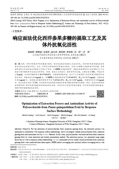
赵丽明，郭煦遥，毛英民，等. 响应面法优化西洋参果多糖的提取工艺及其体外抗氧化活性[J]. 食品工业科技，2023，44（13）：160−166. doi: 10.13386/j.issn1002-0306.2022070318ZHAO Liming, GUO Xuyao, MAO Yingmin, et al. Optimization of Extraction Process and Antioxidant Activity of Polysaccharide from Panax quinquefolium Fruit by Response Surface Methodology[J]. Science and Technology of Food Industry, 2023, 44(13):160−166. (in Chinese with English abstract). doi: 10.13386/j.issn1002-0306.2022070318· 工艺技术 ·响应面法优化西洋参果多糖的提取工艺及其体外抗氧化活性赵丽明1，郭煦遥2，毛英民1，赵大庆1，黄宝泰2，李佳奇1，刘　莉2, *，齐　滨2,*（1.长春中医药大学吉林省人参科学研究院，吉林长春 130117；2.长春中医药大学药学院，吉林长春 130117）摘　要：目的：对西洋参果实中的多糖进行提取，结合响应面法对提取工艺进行优化，并对西洋参果多糖是否具有体外抗氧化活性进行研究。

方法：本研究以新鲜的西洋参果实为原料，采用了水提醇沉法提取其中的多糖。

用单因素实验以及响应面法对提取工艺进行了优化。

从DPPH 自由基清除率、羟基自由基清除率以及还原能力三个方面进行果多糖的体外抗氧化活性研究。

结果：最佳工艺参数为：提取时间为2.5 h ，乙醇浓度为80%，料液比为1:16 g/mL ，此时的多糖得率为29.47%±0.65%，与模型预测值相当。

1、下载文档前请自行甄别文档内容的完整性，平台不提供额外的编辑、内容补充、找答案等附加服务。
2、"仅部分预览"的文档,不可在线预览部分如存在完整性等问题,可反馈申请退款(可完整预览的文档不适用该条件!)。
3、如文档侵犯您的权益，请联系客服反馈,我们会尽快为您处理(人工客服工作时间：9:00-18:30)。

A Novel Preprocessing Method Using Hilbert Huang Transform for MALDI-TOF and SELDI-TOF Mass Spectrometry DataLi-Ching Wu1,2*,Hsin-Hao Chen1,Jorng-Tzong Horng1,3,4,Chen Lin1,Norden E.Huang1,5,Yu-Che Cheng6,Kuang-Fu Cheng7,81Graduate Institute of System Biology and Bioinformatics,National Central University,Jhongli,Taiwan,2Research Center for Biotechnology and Biomedical Engineering, National Central University,Jhongli,Taiwan,3Department of Computer Science and Information Engineering,National Central University,Jhongli,Taiwan,4Department of Bioinformatics,Asia University,Wu-feng,Taiwan,5Research Center for Adaptive Data Analysis,National Central University,Jhongli,Taiwan,6Proteomics Laboratory, Cathay Medical Research Institute,Cathay General Hospital,Xizhi,Taiwan,7Graduate Institute of Statistics,National Central University,Jhongli,Taiwan,8Graduate Institute of Statistics,China Medical University,Taichung,TaiwanAbstractMotivation:Mass spectrometry is a high throughput,fast,and accurate method of protein ing the peaks detected in spectra,we can compare a normal group with a disease group.However,the spectrum is complicated by scale shifting and is also full of noise.Such shifting makes the spectra non-stationary and need to align before comparison.Consequently,the preprocessing of the mass data plays an important role during the analysis process.Noises in mass spectrometry data come in lots of different aspects and frequencies.A powerful data preprocessing method is needed for removing large amount of noises in mass spectrometry data.Results:Hilbert-Huang Transformation is a non-stationary transformation used in signal processing.We provide a novel algorithm for preprocessing that can deal with MALDI and SELDI spectra.We use the Hilbert-Huang Transformation to decompose the spectrum and filter-out the very high frequencies and very low frequencies signal.We think the noise in mass spectrometry comes from many sources and some of the noises can be removed by analysis of signal frequence domain.Since the protein in the spectrum is expected to be a unique peak,its frequence domain should be in the middle part of frequence domain and will not be removed.The results show that HHT,when used for preprocessing,is generally better than other preprocessing methods.The approach not only is able to detect peaks successfully,but HHT has the advantage of denoising spectra efficiently,especially when the data is complex.The drawback of HHT is that this approach takes much longer for the processing than the wavlet and traditional methods.However,the processing time is still manageable and is worth the wait to obtain high quality data.Citation:Wu L-C,Chen H-H,Horng J-T,Lin C,Huang NE,et al.(2010)A Novel Preprocessing Method Using Hilbert Huang Transform for MALDI-TOF and SELDI-TOF Mass Spectrometry Data.PLoS ONE5(8):e12493.doi:10.1371/journal.pone.0012493Editor:William C.S.Cho,Queen Elizabeth Hospital,Hong KongReceived November26,2009;Accepted August5,2010;Published August31,2010Copyright:ß2010Wu et al.This is an open-access article distributed under the terms of the Creative Commons Attribution License,which permits unrestricted use,distribution,and reproduction in any medium,provided the original author and source are credited.Funding:This project is supported by the Cathay General Hospital(.tw)and National Central University(.tw)Collabaration Project number97CGH-NCU-A1and National Science Council Project number98-2627-M-008-003.The funders had no role in study design,data collection and analysis, decision to publish,or preparation of the manuscript.Competing Interests:The authors have declared that no competing interests exist.*E-mail:richard@.twIntroductionMass spectrometry is currently used to explore protein profiles expressed under different physiological and pathophysiological conditions[1].Moreover,recent progress has opened up new avenues for tumor-associated biomarker discovery[2].A mass spectrum of a sample is a profile representing the distribution of components by mass-to-charge ratio.Spectra of tissues or fluids, like serum,are studied for possible profile changes that further disease diagnosis.Matrix assisted laser desorption ionization (MALDI)and surface-enhanced laser desorption ionization (SELDI)time of flight(TOF)are the two commonly techniques used to generate profiles from experimental samples.The chief feature of mass spectra is the peaks detected in terms of their intensity values and time of flight values.Further peak identi-Since each spectrum contains ten thousands of time of flight points with various intensities,noise in the spectra is unavoidable. Therefore,it is important to develop a suitable algorithm for data preprocessing that improves performance when analyzing spectra.Recently,various data preprocessing methods have been used and these usually comprise several steps.First,baseline subtraction is often used to rescale the plots with the aims of removing systematic artifacts produced by small clusters of matrix material[4].Next,denoising attempts to remove noise signals that are added to the true spectra from the matrix material and by sample contaminants(chemical noise)together with noise caused by the physical characteristics of the machine(electrical noise)[5,6].Furthermore,alignment is a required for combining unusual groups of data together.The same peak may be present,to unavoidable inaccuracy in the spectrum.Peak detection is still necessary across every method and is a key feature of preprocess-ing the data.It is necessary to detect each peak by relying on their peak intensity and time of flight.Finally,normalization helps us to have a uniform format for the analysis of the data and this corrects any systematic variation between the different spectra [7].There are many studies that have described preprocessing of mass spectrum data [6,8,9,10,11,12,13]and have explored their approach’s influence on the raw data.In the study of Meuleman,Engwegen et al.[14],they compared various different algorithms that can be used for normalization.In another,Beyer,Walter et al.[15]compared the performance of the package ‘‘Ciphergen Express Software 3.0’’,which is produced by Ciphergen against the ‘‘R package PROcess’’.Recently,Cruz-Marcelo,Guerra et al.[7]compared a number of widely used algorithms,namely ‘‘Pro-teinChip ßSoft-ware 3.1’’(Ciphergen Biosystems),‘‘Biomarker’’Wizard (Ciphergen Biosystems),‘‘PROcess’’,which was written by Xiaochun Li as the ‘‘BioConductor’’package,‘‘Cromwell’’written using Matlab scripts,‘‘SpecAlign’’developed by Wong,Cagney et al.[11],and ‘‘MassSpecWavelet’’developed by Du,Kibbe et al.[12]as a ‘‘BioConductor’’package.Nevertheless,although many preprocessing methods have been put forward,the preprocessing algorithm can still be improved.In the past,the scientists have tried to compute a formula for noise that consists of chemical and machine noise using a statistical method and then constructing a model based on this.However,the chemical noise is generally due to true peaks,namely organic acids,which are part of the matrix used in mass spectrometry.The matrix has two purposes:ionization and protection.It provides hydrogen ions to the peptides or proteins,which are then allowed to undergo ionization and flight in the machine.In addition,the matrix protects the peptide or protein during the laser flash.Matrix noise usually appears in the low mass-to-charge ratio regions (,1000DA).Nonetheless,we need to understand that peaks in the low mass-to-charge ratio region are not only due to chemical noise but also contain true signal peaks.If we mixed the chemical noise with the machine noise as part of preprocessing,we might conclude that the noise strongly affecting the low mass-to-charge ratio region is due to the abundance of organic acids in this region.However,if we take into account the difference between chemical and machine noise when we analyze the spectra,we ought to be able to separate chemical noise from machine noise;this is because the peaks in the low mass-to-charge ratio regions are due to the organic acids and thus distinct from machine noise.The machine noise may come from variety of different sources includes air dust,electric detection limitation,electric white noise,and even earth magnetic field.These noises may not have fixed frequences since the m/z value have measurement shifting problem.In the present study we present a novel preprocessing method using Hilbert Huang transformation (HHT)that is used to decompose a non-linear and non-stationary model.By using HHT,the data can be decomposed into different trends which separate some noises from signals.The main advantage of HHT is non-stationary.It does not make strong assumption that the signal respond to the axis to be stationary distributed.Since the m/z axis exist shifting problem,the HHTcanFigure ponents decomposed using HHT.HHT decomposes the spectrum into sixteen components.From bottom to top,we call them as C1,C2,and so on.Summation of all components can is the original spectrum.eliminate more non-stationary noises than stationary method such as wavelet.The disadvantage is the calculation time will much longer then stationary method.We then compare our algorithm with three familiar preprocessing methods and with another algorithm that has been suggested by Cruz-Marcelo, Guerra et al.[7].Figure2.Before and after HHT preprocessing.(a)The average of fifty ovarian cancer datasets.There are greater amounts of noise in the low region than in the high region.The scale is approximately ten to the ninth power.(b)The same figure after using the Hilbert Huang transformation formula and the various modifications carried out after preprocessing.When comparing with(a),it can be seen that the chief peaks and the profile are maintained.Materials and MethodsHilbert Huang transformationHHT[16]is an adaptive data analysis method for non-linear and non-stationary processes.We use HHT to define the trends in a spectrum.In the past,we have defined the trend that represents the baseline and the noise as a straight line,which is then fitted to the spectrum;then we removed the straight line to yield a zero-mean residue.However,such trends are not suitable for non-linear data and the real-world.Noise exists non-linearly and is non-stationary.In reality,the line is non-linear and non-stationary when we try to rescale spectra.The main feature of the HHT is the empirical mode decomposition(EMD)method with which any complicated data can be decomposed into a finite and often a small number of components called intrinsic mode functions(IMF).We define the IMF if the intrinsic mode of oscillation satisfies two conditions: firstly that the number of the extrema and the number of the zero-crossings must either equal or differ at most by one in the whole dataset and,secondly,the mean value of the envelope defined by the local minima is zero at any point.The IMFs by the EMD method are chiefly obtained by an approach called the sifting process.Actually,the number of IMFs is closed to log2N where N denotes the total number of data points.The sum of all IMFs is equal to the original data.We chose one of the ovarian cancer datasets from the National Cancer Institute published by Kwon,Vannucci et al.[6]to undergo the HHT process.Sixteen IMF components were identified while applying sifting process to our data.As is shown in the Figure1,the later components,namely the ones from the fourteenth IMF to the sixteenth IMF,can be removed for the purpose of rescaling;we also removed the components from first IMF to sixth IMF for the purpose of denoising.Thus a significant part of the chemical noise can be separated from the main spectrum by removing the first components.Subsequent ModificationsIn addition to using the HHT for de-noising,the baseline needs to be adjusted.Here we apply SpecAlign software for baseline estimation,which is available at / ,JWONG/SPECALIGN[11].For removing the baseline,the software has two user-defined options:window size of the baseline and subtraction of the baseline.We set the window size as20,and then we remove the baseline.After baseline subtraction,we rescaled the spectrum to positive.We moved the whole spectrum to be positive by changing the intensity values.However,we did not change other parameters.Our method,which we have called HHTMass,consists of using the Hilbert Huang transformation for denoising followed by modification of the spectrum by baseline subtraction and rescaling.The spectrum before and after the HHT preprocessing are shown in Figure2(a)and2(b)(spectrum source shown in data source section).Peak detectionWe apply three methods,namely MassSpecWavelet[12], SpecAlign[11],and PROcess[9]for peak detection.The major feature of MassSpecWavelet is that the package does not contain any preprocessing method.According to Cruz-Marcelo,Guerra et al.[7],MassSpecWavelet has the best performance in terms of peak detection.PROcess is a BioConductor package by Li[9],which has high quality of peak quantification.SpecAlign,written by Wong [11],is a well known spectrum analysis software package;it has the useful property of containing many user defined options that increase choice.The preprocessing methodology linked toMassSpec-Wavelet Figure3.Sample pancreatic cancer data.Original data of pancreatic cancer provided by Ge and Wong(2008).In this dataset,there is more noise where the peaks exist.was designated as HHTMass1,that linked to SpecAlign as HHTMass2,and that linked to PROcess as HHTMass3.Data sourceTwo different samples are used in this study.Ovarian cancer data is acquired from the authors of[6]in National Cancer Institute. Serum samples from women diagnosed with ovarian cancer and women hospitalized for other conditions were collected at the Mayo Clinic from1980to1989.The dataset was analyzed by SELDI-TOF MS using the CM10chip type[17].The ProteinChip Biomarker System was used for protein expression profiling.The spectrum has two properties,m over z and intensity.The dataset consists of fifty samples after1986.The m over z ranges are between58Da and101453Da.The intensity ranges are between23.27E7and2.14E9.Based on the results of Cruz-Marcelo,Guerra et al.et al.[7]and Kwon,Vannucci et al.[6],in this study we examined the m over z range from2000Da to 15000Da.Each sample has21552points.Figure4.Different peaks detected by different peak selection method.(a)The ovarian cancer dataset preprocessed by HHTMass1.The chosen area is from4000DA to6000DA.The figure is the original spectrum and the circled points are the peaks detected by HHTMass1.HHTMass1 detected32peaks in this region.(b)The ovarian cancer dataset preprocessed by HHTMass2.The chosen area is from4000DA to6000DA.The figure is the original spectrum and the circled points are the peaks detected by HHTMass2.HHTMass1detected17peaks in this region.(c)The ovarian cancer dataset preprocessed by HHTMass3.The chosen area is from4000DA to6000DA.The figure is the original spectrum and the circled points are the peaks detected by HHTMass3.The largest peak in the region between5000DA and6000DA was not detected by HHTMass3.HHTMass3detected18 peaks in this region.doi:10.1371/journal.pone.0012493.g004Figure5.Spectrum data after using HHT preprocessing.The data after using Hilbert Huang transformation without modification.The high frequency noises are removed.doi:10.1371/journal.pone.0012493.g005Table1.The amount of the peaks detected in our three algorithms.Algorithm Total region Region A Region B Region C Region D Region E Region F Region G HHTMass121835322721443821HHTMass2801817611893HHTMass310821181913141310The table shows the results of different preprocessing methods.Region A represents the m over z value between2000DA and4000DA.Similarly,B,C,D,E,F,and G represent the region of4000DA to6000DA,6000DA to8000DA,8000DA to10000DA,10000DA to12000DA,12000DA to14000DA,and14000DA to15000DA,whereasAs we see the Figure2(a),the spectrum is full of noise, especially in low m over z value region.Several different denoising methods have been developed to handle this type of data[6,13,18,19].In general,these approaches use a simulated model for comparing the performance of preprocessing methods. However,the above preprocessing methods seem to be pre-justified in their model.The real distribution of noise is more irregular in real experiments because we cannot understand completely how electrical and chemical noise is generated in a spectrum.Therefore,in this study we compared our approach with the other methods using real data rather than simulated data.It is well-known that Morris,et al.[20]proposed a model using Gaussian white noise and that Cruz-Marcelo,Guerra et al.[7]proposed the ARMA model.However,there is no evidence to show which model fits real data.The preprocessing methods proposed up to now fit their data and their model.For example, we requested a pancreatic cancer dataset from[21]and compared it to the ovarian cancer data.In the Figure3,the pancreatic cancer spectrum has high amounts of noise in the regions where peaks exist,which is different from[6],where the noise is greater in the low region.Therefore,approaches to constructing the model cannot be uniform.In this context then it is clear that real data is the best target when carrying out comparisons.In fact,while processing the mass spectrum data,we substituted the scale of time of flight for the scale of m/z values.The transform was carried out according to the formula(1).m=z U ~sign t{t0ðÞ:a:t{t0ðÞ2:bð1ÞHere t denotes the time of flight,U=25000,a=3.36E8, b=0.00235,and t0=3.7071E-7.A single spectrum has21 551data points in our experiments[6].After the above pre-processing step,we should be able to compare the spectra and distinguish biomarkers that identify the differences between healthy and diseased individuals.Methods of comparisonPreviously,scientists have compared performance mainly in terms of peak detection and peak quantification.Peak detection means that we compare the number of detected prevalent peaks between the different preprocessing methods.Peak quantification means the differences in m over z values and the differences in intensity between the detected prevalent peaks and original spectrum are ing the three methods in the present study,the number of detected peaks is quite different.As can be seen in Figure4(a)and Figure4(b),HHTMass1detects the most peaks and HHTMass2detects the least peaks;furthermore, Figure4(c)shows that HHTMass3failed to detect the biggest peak in the B(4000DA,6000DA)region.Therefore,it is clear that the number of the peaks detected is not the only reference material that we need to consider when assessing the performance of preprocessing methods and these are explored below.In this context,we would expect that the profile of the preprocessed spectrum should be similar to that of the original, especially the intensity of the obvious peaks.However,part of preprocessing aims at decreasing the large scale of the spectrum. The scale of the ovarian dataset is very large and is full of complex signals.With such a large scale,noise exists to a very significant extent across the spectrum.The best approach to this problem is to maintain the exterior of the profile;therefore we decreased the scale by about50%in proportion to the original. Figure2(a)represents the original data and Figure2(b) represents the data after using Hilbert Huang transformation formula and other modifications during preprocessing.When the two figures are compared,it can be seen that the chief peaks and the exterior profile of the spectrum are maintained.Nevertheless, the approach has attempted to remove the signaling errors due to machine and chemical noise.Although we have tried to maintain the exterior profile of the spectrum,we still need to determine whether the peaks present in the preprocessed spectrum are noise or true signals.Finally,when correcting spectra and for visual calibrating purposes,it is better if the baseline of the spectrum is moved to the origin point of the coordinates.Therefore,the final goals of a preprocessing method include retaining the spectrum profile,removing noise,and adjusting the baseline.Using a comparison of peak numbers is only one way of assessing the performance of a preprocessing method.In this study we not only calculated the number of detected peaks but also assessed the real location of the peaks in the spectrum.When the dataset has a large scale,which is the case with the present dataset, peak quantification as an assessment method needs to be replaced because once we have rescaled the spectrum but maintained the spectrum profile then the relative intensity of the peaks becomes meaningless.Therefore,in this analysis,we used visual comparison as the means of assessing performance rather than peak quantification.In this context,the visual comparison involves comparing the distance between the peaks and appearance of theFigure6.Different peaks detected by different peak selection method on full spectrum us HHTMass.(a)The ovarian cancer dataset preprocessed by HHTMass1.The detected peaks cover most raised peaks.HHTMass1detected218peaks in the whole region.(b)The ovarian cancer dataset preprocessed by HHTMass2.HHTMass2tends to detect the more obvious peaks.This algorithm detected80peaks across the whole region.(c)The ovarian cancer dataset preprocessed by HHTMass3.HHTMass3misses the third largest peak close to6000DA.HHTMass3detected108peaks in the whole region.doi:10.1371/journal.pone.0012493.g006Table2.The amount of the peaks detected in severalpopular algorithms.RegionAlgorithm All A B C D E F GPRO11454624191816166PRO2114402381213144HHTMass3(HHT+PRO)10821181913141310MSW1885139252422207HHTMass1(HHT+MSW)21835322721443821PROMSW1985437332523188SpecAlign1866743211816147HHTMass2(HHT+Specalign)801817611893PRO1and PRO2mean different way to estimate the baseline in PROcess.MSWis the abbreviation of MassSpecWavelet.PROMSW is the combinationpreprocessing method of PROcess for peak quantification andMassSpecWavelet for peak detection.HHTMass1,HHTMass2,HHTMass3onlyreplace the preprocess method and use the original peak selection methodrespectively.Figure7.Peaks detected by PRO1and PRO2.(a)The ovarian cancer dataset preprocessed by PRO1.PRO1missed the three largest peaks.PRO1 detected145peaks in the whole region.(b)The ovarian cancer dataset preprocessed by PRO2.PRO2misses the two largest peaks.PRO2detected 114peaks in the whole region.doi:10.1371/journal.pone.0012493.g007Cruz-Marcelo,Guerra et al.[7]suggested several methods of dealing with a spectrum and these included MassSpecWavelet[12] for peak detection and PROcess[9]for peak quantification.Cruz-Marcelo,Guerra et al.[7]suggested that a combined method involving both MassSpecWavelet and PROcess could be used.In addition to the above,we also used the commonly available tool SpecAlign.[11].Thus,in this analysis,we compare our preprocessing method with those mentioned above and these are abbreviated to SpecA-lign SA,MassSpecWavelet MSW and PROcess PRO as shown in the Result sections.ResultsWe computed the average of fifty original ovarian cancer spectrums and then identified with symbols where the various methods detected peaks using the average raw data.This allows performance to be more obviously compared.Our preprocessing method was then utilized and the best peak detection system identified;then we compare the results of five well known preprocessing methods with our preprocessing approach. Results after Hilbert Huang transformation and modificationWe used HHT to preprocess the ovarian cancer data.The raw data is obviously full of noise,especially in the low region.HHT decomposed each spectrum into sixteen components.We called these components C i for i[1,2,…,16](Figure1).Figure1 indicates that the components from C1to C7contain mostly noise, while components from C14to C16are associated with the trend of the spectrum.When these components are removed(Figure5) then the wave pattern become much smoother.After HHT,the spectrum is made up of both positive and negative parts.Based on the results of the modification shown in Figure2(b),we subtract the baseline from spectra and rescale the spectrum to be positive. Results of a comparison between our methodsAfter HHT and the follow up modifications,we used MassSpecWavelet,SpecAlign,and PROcess for peak detection. It should be note that these algorithms were not used for preprocessing,which was only carried out by HHTMass.We marked an area on the original spectrum and separate this into seven regions for convenience.As shown in Table1,HHTMass1 detected the most number of peaks,namely218.In contrast, HHTMass2detected the least number of peaks.Nevertheless, although HHTMass2(Figure6(b))detected the least number of peaks,those detected covered all of the obvious peaks in the original spectrum.This differed from HHTMass3,which missed several significant peaks(Figure6(c)).Based on the above results, we chose HHTMass1and HHTMass2as our approaches to spectrum analysis and rejected HHTMass3.Results of comparison between our method and other methodsAccording to Cruz-Marcelo,Guerra et al.[7],the algorithms PROcess[9]and MassSpecWavelet[12]gave the best perfor-mance in terms of peak quantification and peak detection.The authors then suggest a combination of PROcess for peak quan-tification and MassSpecWavelet for peak detection.In addition, SpecAlign[11]is a well-known software package used to handle mass spectrum data.Therefore,we compared our algorithms, HHTMass1and HHTMass2,with PROcess,MassSpecWavelet, SpecAlign,and a combination of PROcess and MassSpecWavelet [7].The combination of PROcess and MassSpecWavelet is abbreviated to PROMSW in this study.PROcess used two methods to estimate the baseline.One uses local interpolation and the other uses local regression.Based on Cruz-Marcelo,Guerra et al.[7],the former was designated PRO1 and the latter PRO2.Table2shows that HHTMass1is able to detect the most peaks and HHTMass2detects the least peaks. When Figure7(a)and Figure7(b)are examined,PRO1and PRO2miss the two most obvious peaks whereas the other algorithms detect these peaks.MSW(Figure8(a))and PROMSW Figure8(b))seem to cover most of the obvious peaks on visual assessment.However,as we amplify the spectra, some marked peaks are counted twice with MSW and PROMSW. SpecAlign(Figure8(c))performs well in terms of visual assessment;however,as can be seen from Table2,SpecAlign detects more peaks than the other approaches in the range between2000Da and6000Da.If the associated documents produced by BIO-RAID Laboratories for the Proteinchip matrices (ProteinChip H)are examined,there are three common Pro-teinchip matrices that are used in SELDI technology,namely: N Alpha-cyano-4-hydroxycinnamic acid(CHCA),which enables efficient laser desorption and ionization of small proteins (,30kDa).N Sinapinic acid(SPA),which enables efficient laser desorption and ionization of larger proteins(10–150kDa).N EAM-1,a proprietary formulation,that enables efficient laser desorption and ionization of glycosylated proteins and proteins in the15–50kDa rangeAs suggested by the manufacturer’s documents,low regions such as2000Da to6000Da are usually ignored due to the large amount of noise and the restrictions caused by the Proteinchip matrices and samples.Therefore,when looked at from either the statistical point of view[6],or the biological point of view,theFigure8.Peaks detected by other methods.(a)The ovarian cancer dataset preprocessed by MassSpecWavelet.MassSpecWavelet produced some redundancies when detecting peaks.For example,the biggest peak is detected twice.MassSpecWavelet detected188peaks.(b)The ovarian cancer dataset preprocessed by PROMSW.PROMSW produced some redundancies when detecting the peaks and the result is similar to Figure8(a).(c)The ovarian cancer dataset preprocessed by SpecAlign.The peaks detected by SpecAlign are concentrated in the region between2000DA and 6000DA.SpecAlign detected186peaks in the whole region.doi:10.1371/journal.pone.0012493.g008Table3.CPU time of different approach(in seconds).Algorithm Sample No.HHT MASCAP(wavelet)Plasma P_14084.77778.724561Plasma P_23949.68338.996664Plasma P_33908.31518.151383Plasma P_44049.26627.785374Plasma P_53939.03118.117013Average3986.21478.4094196doi:10.1371/journal.pone.0012493.t003。