数字信号实验第四章答案(DOC)

合集下载

(完整word版)电子技术基础数字部分第五版康光华主编第4章习题答案

第四章习题答案4.1.4 试分析图题4.1.4所示逻辑电路的功能。

解：（1）根据逻辑电路写出逻辑表达式：()()L A B C D =⊕⊕⊕ （2）根据逻辑表达式列出真值表：由真值表可知，当输入变量ABCD 中有奇数个1时，输出L=1，当输入变量中有偶数个1时，输出L=0。

因此该电路为奇校验电路。

4.2.5 试设计一个组合逻辑电路，能够对输入的4位二进制数进行求反加1 的运算。

可以用任何门电路来实现。

解：（1）设输入变量为A 、B 、C 、D ，输出变量为L3、L2、L1、L0。

（2）根据题意列真值表：（3）由真值表画卡诺图（4）由卡诺图化简求得各输出逻辑表达式()()()3L AB A C AD ABCD A B C D A B C D A B C D =+++=+++++=⊕++ ()()()2L BC BD BCD B C D B C D B CD =++=+++=⊕+ 1L CD CD C D =+=⊕0L D =（5）根据上述逻辑表达式用或门和异或门实现电路，画出逻辑图如下：A B CDL 3L 2L 1L 04.3.1判断下列函数是否有可能产生竞争冒险，如果有应如何消除。

（2）(,,,)(,,,,,,,)2578910111315L A B C D m =∑ （4）(,,,)(,,,,,,,)4024612131415L A B C D m =∑解：根据逻辑表达式画出各卡诺图如下：（2）2L AB BD =+，在卡诺图上两个卡诺圈相切，有可能产生竞争冒险。

消除办法：在卡诺图上增加卡诺圈（虚线）包围相切部分最小项，使2L AB BD AD =++，可消除竞争冒险。

（4）4L AB AD =+，在卡诺图上两个卡诺圈相切，有可能产生竞争冒险。

消除办法：在卡诺图上增加卡诺圈（虚线）包围相切部分最小项，使4L AB AD BD =++，可消除竞争冒险。

4.3.4 画出下列逻辑函数的逻辑图，电路在什么情况下产生竞争冒险，怎样修改电路能消除竞争冒险。

数字信号处理第四章习题

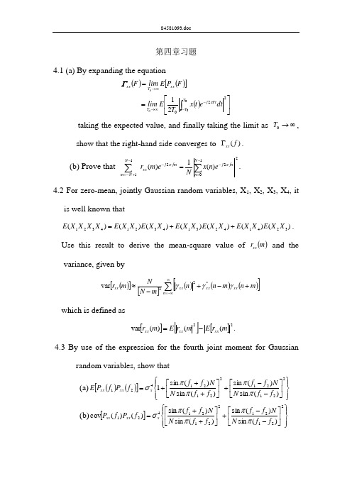
第四章习题4.1 (a) By expanding the equation()()[]()⎥⎦⎤⎢⎣⎡==⎰--∞→∞→2200021T T Ft j T xx T xx dt e t x T E lim F P E lim F 00πΓ taking the expected value, and finally taking the limit as ∞→0T ,show that the right-hand side converges to )(f xx Γ.(b) Prove that2102211)(1)(∑∑-=---+-==N n fn j fm j N N m xx en x N e m r ππ.4.2 For zero-mean, jointly Gaussian random variables, X 1, X 2, X 3, X 4, itis well known that)()()()()()()(3241423143214321X X E X X E X X E X X E X X E X X E X X X X E ++=. Use this result to derive the mean-square value of ()m r xx and the variance, given by()[][]()()()[]∑∞-∞=+-+-≈n xx xx xx xx m n m n n m N N m r γγγ*22varwhich is defined as[][][]22(()(var m r E m r E m r xx xx xx -=. 4.3 By use of the expression for the fourth joint moment for Gaussianrandom variables, show that(a)()()[]⎪⎭⎪⎬⎫⎪⎩⎪⎨⎧⎥⎦⎤⎢⎣⎡--+⎥⎦⎤⎢⎣⎡+++=2212122121421)(sin )(sin )(sin )(sin 1f f N N f f f f N N f f f P f P E x xx xx ππππσ (b)[]⎪⎭⎪⎬⎫⎪⎩⎪⎨⎧⎥⎦⎤⎢⎣⎡--+⎥⎦⎤⎢⎣⎡++=2212122121421)(sin )(sin )(sin )(sin )()(cov f f N N f f f f N N f f f P f P x xx xx ππππσ(c)[]⎪⎭⎪⎬⎫⎪⎩⎪⎨⎧⎪⎪⎭⎫ ⎝⎛+=242sin 2sin 1)(var f N fN f P x xx ππσ under the condition that the sequence ()n x is a zero-mean white Gaussian noise sequence with variance 2x σ.4.4 Generalize the results in Problem 4.3 to a zero-mean Gaussian noiseprocess with power density spectrum )(f xx Γ, as given by()[]()⎥⎥⎦⎤⎢⎢⎣⎡⎪⎪⎭⎫ ⎝⎛+Γ=222sin 2sin 1var f N fN f f P xx xx ππ (Hint: Assume that the colored Gaussian noise process is the output of a linear system excited by white Gaussian noise.)4.5 Show that the periodogram values at frequencies,1,1,0,/-==L k L k f k given by (4.1.35), can be computed by passing the sequence through a bank of L IIR filters, where each filter has an impulse response )()(/2n u e n h N nk j k π-= and then computing the magnitude-squared value of the filter outputs at n=N. Note that each filter has a pole on the unit circle at the frequency f k .4.6 The Bartlett method is used to estimate the power spectrum of asignal x(n). We know that the power spectrum consists of a single peak with a 3 dB bandwidth of 0.01 cycle per sample, but we do not know the location of the peak.(a) Assuming that N is large, determine the value of M=N/K so thatthe spectral window is narrower than the peak.(b) Explain why it is not advantageous to increase M beyond thevalue obtained in part (a).4.7 The N-point DFT of a random sequence x(n) is ∑-=-=10/2)()(N n N nk j e n x k X π.Assume that E[x(n)]=0 and E[x(n)x(n+m)]=)(2m w δσ (in other words,x(n) is a white noise process).(a) Determine the variance of X(k).(b) Determine the autocorrelation of X(k).4.8 An AR(2) process is described by the difference equation)()2(81.0)(n n x n x ω+-=, where w(n) is a white noise process withvariance 2ωσ.(a) Determine the parameters of the MA(2), MA(4), and MA(8)models that provide a minimum mean-sequare error fit to thedata x(n).(b) Plot the true spectrum and those of the MA (q), q=2,4,8spectra and compare the results. Comment on how well theMA(q) models approximate the AR (2) process.4.9 An MA (2) process is described by the difference equation )2(81.0)()(-+=n n n x ωω, where w(n) is a white noise process withvariance 2ωσ.(a) Determine the parameters of the AR(2), AR(4), and AR(8)models that provide a minimum mean-square error fit to the data x(n).(b) Plot the true spectrum and those of the AR(p), p=2,4,8, andcompare the results. Comment on how well the AR(p) modelsappoximate the MA (2) process.4.10 The autocorrelation sequence for an AR process x(n) ismxx m ⎪⎭⎫ ⎝⎛=41)(γ (a) Determine the difference equation for x(n)(b) Is your answer unique? If not, give any other possiblesolutions.4.11 Suppose that we represent an ARMA(p,q) process as a cascade ofan MA(q) followed by an AR(p) model. The input-output equation for the MA(q) model is ∑=-=qk k k n w b n v 0)()(, where w(n) is a whitenoise process. The input-output equation for the AR(p) model is∑==-+pk k n v k n x a n x 1)()()((a) By computing the autocorrelation of v(n), show thatq m d b b m mq k m w m k k w vv ≤≤==∑-=+0)(022σσγ(b) Show that 1)()(00=+=∑=a k m a m pk vx k vv γγ4.12 Suppose that the AR(2) process in Problem 4.8 is corrupted by anadditive white noise process v(n) with variance 2v σ. Thus, we havey(n)=x(n)+v(n)(a) Determine the difference equation for y(n) and thusdemonstrate that y(n) is an ARMA(2,2) process. Determinethe coefficients of the ARMA process.(b) Generalize the result in part (a) to an AR(p) process∑=+--=pk k n w k n x a n x 1)()()( and )()()(n v n x n y +=.4.13 The harmonic decomposition problem considered by Pisarenko maybe expressed as the solution to the equationa a a Γa H w yy H 2σ=The solution for a may be obtained by minimizing the quadratic form a Γa yy H subject to the constraint that a a H =1. The constraint can be incorporated into the performance index by means of a Lagrange multiplier. Thus the performance index becomes()a a a Γa H yy H 1-+=λζ.By minimizing ζ with respect to a , show that this formulation is equivalent to the Pisarenko eigenvalue problem given in (4.4.9), with the Lagrange multiplier playing the role of the eigenvalue. Thus,show that the minimum of ζ is the minimum eigenvalue 2w σ.4.14 The autocorrelation of a sequence consisting of a sinusoid withrandom phase in noise is)(2cos )(21m m f P m w xx δσπγ+=where 1f is the frequency of the sinusoidal, P its power, and 2w σthe variance of the noise. Suppose that we attempt to fit an AR(2) model to the data.(a) Determine the optimum coefficients of the AR(2) model as afunction of 2w σ and 1f .(b) Determine the reflection coefficients 1K and 2K correspondingto the AR(2) model parameters.(c) Determine the limiting values of the AR(2) parameters and (1K ,2K )as 02→w σ.4.15 This problem involves the use of cross-correlation to detect a signalin noise and estimate the time delay in the signal. A signal x(n) consists of a pulsed sinusoid corrupted by a stationary zero-mean white noise sequence. That is, 10),()()(0-≤≤+-=N n n w n n y n x ,where )(n w is the noise with variance 2w σ and the signal is⎩⎨⎧-≤≤=otherwise M n n A n y ,010,cos )(0ω. The frequency 0ω is known, but the delay 0n , which is a positiveinteger, is unknown, and is to be determined by cross-correlating x(n) with y(n). Assume that 0n M N +>. Let∑-=-=10)()()(N n xy n x m n y m rdenote the cross-correlation sequence between x(n) and y(n). In the absence of noise, this function exhibits a peak at delay 0n m =. Thus,0n is determined with no error. The presence of noise can lead toerrors in determining the unknown delay.(a) For 0n m =, determine ()[]0n r E xy . Also, determine thevariance ()[]0var n r xy , due to the presence of the noise. In bothcalculations, assume that the double-frequency term averages to zero. That is, 0/2ωπ>>M .(b) Determine the signal-to-noise ratio, defined as []{}[])(var )(020n r n r E SNR xy xy = (c) What is the effect of the pulse duration M on the SNR?。

数字信号处理实验答案完整版

数字信号处理实验答案 HEN system office room 【HEN16H-HENS2AHENS8Q8-HENH1688】实验一熟悉Matlab环境一、实验目的1.熟悉MATLAB的主要操作命令。

2.学会简单的矩阵输入和数据读写。

3.掌握简单的绘图命令。

4.用MATLAB编程并学会创建函数。

5.观察离散系统的频率响应。

二、实验内容认真阅读本章附录，在MATLAB环境下重新做一遍附录中的例子，体会各条命令的含义。

在熟悉了MATLAB基本命令的基础上，完成以下实验。

上机实验内容：（1）数组的加、减、乘、除和乘方运算。

输入A=[1 2 3 4]，B=[3 4 5 6]，求C=A+B，D=A-B，E=A.*B，F=A./B，G=A.^B并用stem语句画出A、B、C、D、E、F、G。

clear all;a=[1 2 3 4];b=[3 4 5 6];c=a+b;d=a-b;e=a.*b;f=a./b;g=a.^b;n=1:4;subplot(4,2,1);stem(n,a);xlabel('n');xlim([0 5]);ylabel('A');subplot(4,2,2);stem(n,b);xlabel('n');xlim([0 5]);ylabel('B');subplot(4,2,3);stem(n,c);xlabel('n');xlim([0 5]);ylabel('C');subplot(4,2,4);stem(n,d);xlabel('n');xlim([0 5]);ylabel('D');subplot(4,2,5);stem(n,e);xlabel('n');xlim([0 5]);ylabel('E');subplot(4,2,6);stem(n,f);xlabel('n');xlim([0 5]);ylabel('F');subplot(4,2,7);stem(n,g);xlabel('n');xlim([0 5]);ylabel('G');（2）用MATLAB实现下列序列：a) x(n)= 0≤n≤15b) x(n)=e+3j)n 0≤n≤15c) x(n)=3cosπn+π)+2sinπn+π) 0≤n≤15(n)=x(n+16),绘出四个周期。

北邮数字信号处理第四章附加题答案正式版

1. 请推导出三阶巴特沃思低通滤波器的系统函数，设1/c rad s Ω=。

解：幅度平方函数是：2261()()1A H j Ω=Ω=+Ω令： 22s Ω=- ,则有：61()()1a a H s H s s-=- 各极点满足121[]261,26k j k s ek π-+==所得出的6个 k s 为：15==j es 2321321jes j +-==π12-==πj e s 2321343jes j --==π2321354j es j -==π2321316j es j +==π15==j e s 2321321je s j +-==π12-==πj e s 2321343je s j --==π2321354j es j -==π2321316j es j +==π122))()(()(233210+++=---=s s s k s s s s s s k s H a 1221)(23+++==s s s s H a 代入s=0时, ,可得,故:1=)s (H a 10=k2. 设计一个满足下列指标的模拟Butterworth 低通滤波器，要求通带的截止频率6,p f kHz =，通带最大衰减3,p A dB =，阻带截止频率12,s f kHz =，阻带的最小衰减25s A dB =，求出滤波器的系统函数。

解： 2,2s s p p f f ππΩ=Ω=0.10.1101lg 101N 2lg()s pA A s p⎛⎫- ⎪-⎝⎭≥ΩΩ=4.15取N=5，查表得H(p)为：221()(0.6181)( 1.6181)(1)H p p p p p p =+++++ 因为3,p A dB =所以c p Ω=Ω[]52222()()0.618 1.618cs p c c c c c c H s H p s s s s s =Ω=Ω=⎡⎤⎡⎤+Ω-Ω+Ω-Ω+Ω⎣⎦⎣⎦3. 设计一个模拟切比雪夫低通滤波器，要求通带的截止频率 f p =3kHz ，通带衰减要不大于0.2dB ，阻带截止频率 f s = 12kHz ，阻带衰减不小于 50dB 。

数字电子技术基础(第四版)课后习题答案-第四章

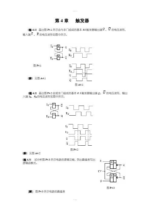
第4章触发器[题4.1]画出图P4.1所示由与非门组成的基本RS触发器输出端Q、Q的电压波形，输入端S、R的电压波形如图中所示。

图P4.1[解]见图A4.1图A4.1[题4.2]画出图P4.2由或非门组成的基本R-S触发器输出端Q、Q的电压波形，输出入端S D，R D的电压波形如图中所示。

图P4.2[解]见图A4.2[题4.3]试分析图P4.3所示电路的逻辑功能，列出真值表写出逻辑函数式。

图P4.3 [解]：图P4.3所示电路的真值表S R Q n Q n+1 0 0 0 0 0 0 1 1 0 1 0 0 0 1 1 0 1 0 0 1 1 0 1 1 1 1 0 0* 1 110*由真值表得逻辑函数式 01=+=+SR Q R S Q nn[题4.4] 图P4.4所示为一个防抖动输出的开关电路。

当拨动开关S 时，由于开关触点接触瞬间发生振颤，D S 和D R 的电压波形如图中所示，试画出Q 、Q 端对应的电压波形。

图P4.4[解] 见图A4.4图A4.4[题4.5] 在图P4.5电路中，若CP 、S 、R 的电压波形如图中所示，试画出Q 和Q 端与之对应的电压波形。

假定触发器的初始状态为Q =0。

图P4.5[解]见图A4.5图A4.5[题4.6]若将同步RS触发器的Q与R、Q与S相连如图P4.6所示，试画出在CP信号作用下Q和Q端的电压波形。

己知CP信号的宽度tw= 4 t Pd 。

t Pd为门电路的平均传输延迟时间，假定t Pd≈t PHL≈t PLH，设触发器的初始状态为Q=0。

图P4.6图A4.6[解]见图A4.6[题4.7]若主从结构RS触发器各输入端的电压波形如图P4.7中所给出，试画Q、Q端对应的电压波形。

设触发器的初始状态为Q=0。

图P4.7[解] 见图A4.7图A4.7R各输入端的电压波形如图P4.8所示，[题4.8]若主从结构RS触发器的CP、S、R、D1S。

试画出Q、Q端对应的电压波形。

数字信号处理第四章答案

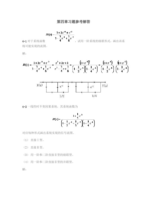
第四章习题参考解答4-1对于系统函数，试用一阶系统的级联形式，画出该系统可能实现的流图。

解：4-2一线性时不变因果系统，其系统函数为对应每种形式画出系统实现的信号流图。

（1）直接Ⅰ型。

（2）直接Ⅱ型。

（3）用一阶和二阶直接Ⅱ型的级联型。

（4）用一阶和二阶直接Ⅱ型的并联型。

解：直接Ⅰ型直接Ⅱ型用一阶和二阶直接Ⅱ型的级联型用一阶和二阶直接Ⅱ型的并联型4-3已知模拟滤波器的传输函数，试用脉冲响应不变法将转换成数字传输函数。

（设采样周期T＝0.5）解：4-4若模拟滤波器的传输函数为，试用脉冲响应不变法将转换成数字传输函数。

（设采样周期T＝1）解：4-5用双线性变换法设计一个三阶的巴特沃滋数字低通滤波器，采样频率，截至频率。

解：,4-6用双线性变换法设计一个三阶的巴特沃滋数字高通滤波器，采样频率，截至频率。

解：，，归一化，4-7用双线性变换法设计一个三阶的巴特沃滋数字带通滤波器，采样频率，上下边带截至频率分别为，。

解：，，，4-8设计一个一阶数字低通滤波器，3dB截至频率为，将双线性变换应用于模拟巴特沃滋滤波器。

解：一阶巴特沃滋，4-9试用双线性变换法设计一低通数字滤波器，并满足：通带和阻带都是频率的单调下降函数，而且无起伏；频率在处的衰减为－3.01dB；在处的幅度衰减至少为15dB。

解：设,则：，通带：,即阻带：，即阶数：，查表得二阶巴特沃滋滤波器得系统函数为双线性变换实现数字低通滤波器4-10一个数字系统的采样频率，已知该系统收到频率为100Hz的噪声干扰，试设计一个陷波滤波器去除该噪声，要求3dB的边带频率为95Hz和105Hz,阻带衰减不小于14dB。

解：，令，，，，设N=2，则。

数字电子技术基础第四章习题及参考答案

数字电子技术基础第四章习题及参考答案第四章习题1．分析图4-1中所示的同步时序逻辑电路，要求：（1）写出驱动方程、输出方程、状态方程；（2）画出状态转换图，并说出电路功能。

CPY图4-12．由D触发器组成的时序逻辑电路如图4-2所示，在图中所示的CP脉冲及D作用下，画出Q0、Q1的波形。

设触发器的初始状态为Q0=0，Q1=0。

D图4-23．试分析图4-3所示同步时序逻辑电路，要求：写出驱动方程、状态方程，列出状态真值表，画出状态图。

CP图4-34．一同步时序逻辑电路如图4-4所示，设各触发器的起始状态均为0态。

（1）作出电路的状态转换表；（2）画出电路的状态图；（3）画出CP作用下Q0、Q1、Q2的波形图；（4）说明电路的逻辑功能。

图4-45．试画出如图4-5所示电路在CP波形作用下的输出波形Q1及Q0，并说明它的功能（假设初态Q0Q1=00）。

CPQ1Q0CP图4-56．分析如图4-6所示同步时序逻辑电路的功能，写出分析过程。

Y图4-67．分析图4-7所示电路的逻辑功能。

（1）写出驱动方程、状态方程；（2）作出状态转移表、状态转移图；（3）指出电路的逻辑功能，并说明能否自启动；（4）画出在时钟作用下的各触发器输出波形。

CP图4-78．时序逻辑电路分析。

电路如图4-8所示：（1）列出方程式、状态表；（2）画出状态图、时序图。

并说明电路的功能。

1C图4-89．试分析图4-9下面时序逻辑电路：（1）写出该电路的驱动方程，状态方程和输出方程；（2）画出Q1Q0的状态转换图；（3）根据状态图分析其功能；1B图4-910.分析如图4-10所示同步时序逻辑电路，具体要求：写出它的激励方程组、状态方程组和输出方程，画出状态图并描述功能。

1Z图4-1011．已知某同步时序逻辑电路如图4-11所示，试：（1）分析电路的状态转移图，并要求给出详细分析过程。

（2）电路逻辑功能是什么，能否自启动？（3）若计数脉冲f CP频率等于700Hz，从Q2端输出时的脉冲频率是多少?CP图4-1112．分析图4-12所示同步时序逻辑电路，写出它的激励方程组、状态方程组，并画出状态转换图。

数字信号处理-原理、实现及应用(第4版) 第四章模拟信号的数字处理

（3）当未知时，由 x(n) 无法恢复原正弦信号。
结论：
正弦信号采样（2）
三点结论：（1）对正弦信号，若 Fs 2 f0 时，不能保证从采样信号恢
复原正弦信号；（2）正弦信号在恢复时有三个未知参数，分别是振幅A、
频率f和初相位，所以，只要保证在一个周期内均匀采样三点，即可由采样信号准确恢复原正弦信号。所以，只要采样频率 Fs 3 f0 ，就不会丢失信息。（3）对采样后的正弦序列做截断处理时，截断长度必须是此正弦序列周期的整数倍，才不会产生频谱泄漏。（见第四章4.5.3节进行详细分析）。
D/A
D/A为理想恢复，相当于理想的低通滤波器，ya (t) 的傅里叶变换为：
Ya ( j) Y (e jT )G( j) H (e jT ) X (e jT )G( j)
保真系统中的应用。
在 |Ω|>π/T ，引入了原模拟信号没有的高频分量，时域上表现
为台阶。
ideal filter
•
-fs
-fs/2 o
• fs/2 fs
f •
2fs
•
•
-fs
-fs/2 o
fs/2
•
fs
•
f
2fs
措施
D/A之前，增加数字滤波器，幅度特性为 Sa(x) 的倒数。
在零阶保持器后，增加一个低通滤波器，滤除高频分量，对信号进行平滑，也称平滑滤波器。
c
如何恢复原信号的频谱？
P (j)
加低通滤波器，传输函数为
G(
j)
T
0
s 2 s 2
s
0
s
X a ( j)
s 2
s c c
s
理想采样的恢复

1、下载文档前请自行甄别文档内容的完整性，平台不提供额外的编辑、内容补充、找答案等附加服务。
2、"仅部分预览"的文档,不可在线预览部分如存在完整性等问题,可反馈申请退款(可完整预览的文档不适用该条件!)。
3、如文档侵犯您的权益，请联系客服反馈,我们会尽快为您处理(人工客服工作时间：9:00-18:30)。

数字信号处理实验报告4线性时不变离散时间系统频域分析一、实验目的通过使用matlab做实验来加强对传输函数的类型和频率响应和稳定性测试来强化理解概念。

4.1 传输函数分析回答:Q4.1 修改程序P3_1去不同的M值，当0<w<2pi时计算并画出式（2.13）所示滑动平均滤波器的幅度和相位谱，代码如下：% Program Q4_1% Frequency response of the causal M-point averager of Eq. (2.13) clear;% User specifies filter lengthM = input('Enter the filter length M: ');% Compute the frequency samples of the DTFTw = 0:2*pi/1023:2*pi;num = (1/M)*ones(1,M);den = [1];% Compute and plot the DTFTh = freqz(num, den, w);subplot(2,1,1)plot(w/pi,abs(h));gridtitle('Magnitude Spectrum |H(e^{j\omega})|')xlabel('\omega /\pi');ylabel('Amplitude');subplot(2,1,2)plot(w/pi,angle(h));gridtitle('Phase Spectrum arg[H(e^{j\omega})]') xlabel('\omega /\pi');ylabel('Phase in radians');所得结果如图示：M=2M=7幅度和相位谱表现出对称性的类型是由于–冲激响应是实数，因此频率响应是周期且对称的，幅度谱是周期甚至对称的，相位响应是周期奇对称。

采用移动平均滤波表示过滤器的类型–低通滤波器Q2.1的结果可以解释为–它是一个低通滤波器，输入是一个两个正弦分量的总和，一个高频和低频。

结果依赖于过滤器的长度，但总的结果是更高频率的正弦输入分量衰减超过较低的频率正弦输入分量。

Q4.2 因果LTI离散时间系统的频率响应曲线得到使用修改后的程序如下:通过此传递函数表示的过滤器类型–带通滤波器Q4.3 对问题的因果LTI离散时间系统的频率响应图q4.3得到使用修改后的程序如下通过此传递函数表示的过滤器类型- 带通滤波器4.2和4.3滤波器的不同在于–幅度谱两个是一样的，但是第二个相位谱不是连续的，原因是它们的极点不是一样的，4.36的极点在单位圆内，所以是稳定的，4.37的极点在单位圆外，所以不稳定。

我会选择4.36滤波器的原因是–因为4.37没有4.36稳定Q4.4 过滤器的群延迟的问题q4.4指定和使用功能如下所示:从图像可以观察到: 这是一个窄阻带的带阻滤波器，在大多数的带通滤波器中，群延迟是恒定的。

Q4.5 4.2和4.3两个滤波器的前100个样本冲击响应的图像如图示：可以得到观察: 4.36给出的滤波器是稳定的，即h[n]是可求和的，并且冲激响应呈指数型衰减，而4.37给出的是不稳定的，所以h[n]随n呈指数型增长。

Q4.6 使用zplane生成式4.36和4.37确定的两个滤波器的零极点图:从图像可以观察到: 上图的极点都在单位圆内，所以是因果稳定的，下图的极点在单位圆外，不是因果稳定。

4.2 传输函数的类型Project 4.2 滤波器P4_1的代码如下：% Program P4_1% Impulse Response of Truncated Ideal Lowpass Filterclf;fc = 0.25;n = [-6.5:1:6.5];y = 2*fc*sinc(2*fc*n);k = n+6.5;stem(k,y);title('N = 13');axis([0 13 -0.2 0.6]);xlabel('Time index n');ylabel('Amplitude');grid;回答:Q4.7 接近于理想低通滤波器的冲击响应的图像：FIR低通滤波器的长度是 - 14P4_1决定低通滤波器长度的语句是– n = [-6.5:1:6.5];控制截止频率的参数是- fc = 0.25;Q4.8 修改程序P4.1，计算并画出式（4.39）所示长度为20，截止频率为wc=0.45的有限冲击响应低通滤波器的冲击响应:% Program Q4_8% Impulse Response of Truncated Ideal Lowpass Filterclf;9fc = 0.45;n = [-9.5:1:9.5];y = 2*fc*sinc(2*fc*n);k = n+9.5;stem(k,y);title('N = 20');axis([0 19 -0.2 0.7]);xlabel('Time index n');ylabel('Amplitude');grid;得到的结果是:Q4.9 必要的修改程序p4_1计算并画出长度与15和0.65的截止频率的FIR低通滤波器的脉冲响应:% Program Q4_9% Impulse Response of Truncated Ideal Lowpass Filterclf;fc = 0.65;n = [-7.0:1:7.0];y = 2*fc*sinc(2*fc*n);k = n+7.0;stem(k,y);title('N = 14');axis([0 14 -0.4 1.4]);xlabel('Time index n');ylabel('Amplitude');grid;得到的图像是：Q4.10 MATLAB计算程序和绘图的FIR低通滤波器的的幅度响应如下：% Program Q4_10% Compute and plot the amplitude response% of Truncated Ideal Lowpass Filterclear;% Get "N" from the user command lineN = input('Enter the filter time shift N: ');% compute the magnitude spectrumNo2 = N/2;fc = 0.25;n = [-No2:1:No2];y = 2*fc*sinc(2*fc*n);w = 0:pi/511:pi;h = freqz(y, [1], w);plot(w/pi,abs(h));grid;title(strcat('|H(e^{j\omega})|, N=',num2str(N)));xlabel('\omega /\pi');ylabel('Amplitude');低通滤波器的幅度相应（若干个n值）:从图像可以得到观察–随着滤波器长度的增加，从通过到不通过变得更加陡峭，我们也可以看到吉布斯现象：当滤波器增加时，幅度相应更加趋向一个理想的低通特征。

然而随着w增长，峰值是增加而不是降低。

P4_2的代码:% Program P4_2% Gain Response of a Moving Average Lowpass Filterclf;M = 2;num = ones(1,M)/M;[g,w] = gain(num,1);plot(w/pi,g);gridaxis([0 1 -50 0.5])xlabel('\omega /\pi');ylabel('Gain in dB');title(['M = ', num2str(M)])回答:Q4.11长度为2的滑动平均滤波器的增益相应的图像：从图中可以看出，3-dB截止频率是-pi/2Q4.12 必要的修改程序p4_2计算并画出一个级联的K长度为2的滑动平均滤波器的增益响应如下：% Program Q4_12% Gain Response of a cascade connection of K% two-point Moving Average Lowpass Filtersclear;K = input('Enter the number of sections K: ');Hz = [1];% find the numerator for H(z) = cascade of K sectionsfori=1:K;Hz = conv(Hz,[1 1]);end;Hz = (0.5)^K * Hz;% Convert numerator to dB[g,w] = gain(Hz,1);% make a horizontal line on the plot at -3 dBThreedB = -3*ones(1,length(g));% make a vertical line on the plot at the% theoretical 3dB frequencyt1 = 2*acos((0.5)^(1/(2*K)))*ones(1,512)/pi;t2 = -50:50.5/511:0.5;plot(w/pi,g,w/pi,ThreedB,t1,t2);grid;axis([0 1 -50 0.5])xlabel('\omega /\pi');ylabel('Gain in dB');title(['K = ',num2str(K),'; Theoretical \omega_{c} = ',num2str(t1(1))]);使用修改后的程序级联部分的增益响应曲线得到如下所示：从图中可以看出，级联的3-dB截止频率是 -0.30015piQ4.13 必要的修改程序p4_2计算高通滤波器的增益响应（4.42）如下: % Program Q4_13% Gain Response of Highpass Filter (4.42)clear;M = input('Enter the filter length M: ');n = 0:M-1;num = (-1).^n .* ones(1,M)/M;[g,w] = gain(num,1);plot(w/pi,g);grid;axis([0 1 -50 0.5]);xlabel('\omega /\pi');ylabel('Gain in dB');title(['M = ', num2str(M)]);通过修改程序，增益响应M=5的曲线为：我们可以得到3-dB 的截止频率在–大约在0.8196piQ4.14 从式子. (4.16) 3-dB截止频率ωc 在0.45π我们可以得到α=0.078702取代α在式子 (4.15) 和(4.17)我们得到的一阶IIR低通和高通滤波器的传递函数，分别给出了H LP(z) =H HP(z) =我们得到的增益响应如图示:从这些图中我们看到，所设计的滤波器满足规格。