Backward inducing and exponential decay of correlations for partially hyperbolic attractors
量子力学英语词汇

1、microscopic world 微观世界2、macroscopic world 宏观世界3、quantum theory 量子[理]论4、quantum mechanics 量子力学5、wave mechanics 波动力学6、matrix mechanics 矩阵力学7、Planck constant 普朗克常数8、wave-particle duality 波粒二象性9、state 态10、state function 态函数11、state vector 态矢量12、superposition principle of state 态叠加原理13、orthogonal states 正交态14、antisymmetrical state 正交定理15、stationary state 对称态16、antisymmetrical state 反对称态17、stationary state 定态18、ground state 基态19、excited state 受激态20、binding state 束缚态21、unbound state 非束缚态22、degenerate state 简并态23、degenerate system 简并系24、non-deenerate state 非简并态25、non-degenerate system 非简并系26、de Broglie wave 德布罗意波27、wave function 波函数28、time-dependent wave function 含时波函数29、wave packet 波包30、probability 几率31、probability amplitude 几率幅32、probability density 几率密度33、quantum ensemble 量子系综34、wave equation 波动方程35、Schrodinger equation 薛定谔方程36、Potential well 势阱37、Potential barrien 势垒38、potential barrier penetration 势垒贯穿39、tunnel effect 隧道效应40、linear harmonic oscillator 线性谐振子41、zero proint energy 零点能42、central field 辏力场43、Coulomb field 库仑场44、δ-function δ-函数45、operator 算符46、commuting operators 对易算符47、anticommuting operators 反对易算符48、complex conjugate operator 复共轭算符49、Hermitian conjugate operator 厄米共轭算符50、Hermitian operator 厄米算符51、momentum operator 动量算符52、energy operator 能量算符53、Hamiltonian operator 哈密顿算符54、angular momentum operator 角动量算符55、spin operator 自旋算符56、eigen value 本征值57、secular equation 久期方程58、observable 可观察量59、orthogonality 正交性60、completeness 完全性61、closure property 封闭性62、normalization 归一化63、orthonormalized functions 正交归一化函数64、quantum number 量子数65、principal quantum number 主量子数66、radial quantum number 径向量子数67、angular quantum number 角量子数68、magnetic quantum number 磁量子数69、uncertainty relation 测不准关系70、principle of complementarity 并协原理71、quantum Poisson bracket 量子泊松括号72、representation 表象73、coordinate representation 坐标表象74、momentum representation 动量表象75、energy representation 能量表象76、Schrodinger representation 薛定谔表象77、Heisenberg representation 海森伯表象78、interaction representation 相互作用表象79、occupation number representation 粒子数表象80、Dirac symbol 狄拉克符号81、ket vector 右矢量82、bra vector 左矢量83、basis vector 基矢量84、basis ket 基右矢85、basis bra 基左矢86、orthogonal kets 正交右矢87、orthogonal bras 正交左矢88、symmetrical kets 对称右矢89、antisymmetrical kets 反对称右矢90、Hilbert space 希耳伯空间91、perturbation theory 微扰理论92、stationary perturbation theory 定态微扰论93、time-dependent perturbation theory 含时微扰论94、Wentzel-Kramers-Brillouin method W. K. B.近似法95、elastic scattering 弹性散射96、inelastic scattering 非弹性散射97、scattering cross-section 散射截面98、partial wave method 分波法99、Born approximation 玻恩近似法100、centre-of-mass coordinates 质心坐标系101、laboratory coordinates 实验室坐标系102、transition 跃迁103、dipole transition 偶极子跃迁104、selection rule 选择定则105、spin 自旋106、electron spin 电子自旋107、spin quantum number 自旋量子数108、spin wave function 自旋波函数109、coupling 耦合110、vector-coupling coefficient 矢量耦合系数111、many-particle system 多子体系112、exchange forece 交换力113、exchange energy 交换能114、Heitler-London approximation 海特勒-伦敦近似法115、Hartree-Fock equation 哈特里-福克方程116、self-consistent field 自洽场117、Thomas-Fermi equation 托马斯-费米方程118、second quantization 二次量子化119、identical particles 全同粒子120、Pauli matrices 泡利矩阵121、Pauli equation 泡利方程122、Pauli’s exclusion principle泡利不相容原理123、Relativistic wave equation 相对论性波动方程124、Klein-Gordon equation 克莱因-戈登方程125、Dirac equation 狄拉克方程126、Dirac hole theory 狄拉克空穴理论127、negative energy state 负能态128、negative probability 负几率129、microscopic causality 微观因果性本征矢量eigenvector本征态eigenstate本征值eigenvalue本征值方程eigenvalue equation本征子空间eigensubspace (可以理解为本征矢空间)变分法variatinial method标量scalar算符operator表象representation表象变换transformation of representation表象理论theory of representation波函数wave function波恩近似Born approximation玻色子boson费米子fermion不确定关系uncertainty relation狄拉克方程Dirac equation狄拉克记号Dirac symbol定态stationary state定态微扰法time-independent perturbation定态薛定谔方程time-independent Schro(此处上面有两点)dinger equation 动量表象momentum representation角动量表象angular mommentum representation占有数表象occupation number representation坐标(位置)表象position representation角动量算符angular mommentum operator角动量耦合coupling of angular mommentum对称性symmetry对易关系commutator厄米算符hermitian operator厄米多项式Hermite polynomial分量component光的发射emission of light光的吸收absorption of light受激发射excited emission自发发射spontaneous emission轨道角动量orbital angular momentum自旋角动量spin angular momentum轨道磁矩orbital magnetic moment归一化normalization哈密顿hamiltonion黑体辐射black body radiation康普顿散射Compton scattering基矢basis vector基态ground state基右矢basis ket ‘右矢’ket基左矢basis bra简并度degenerancy精细结构fine structure径向方程radial equation久期方程secular equation量子化quantization矩阵matrix模module模方square of module内积inner product逆算符inverse operator欧拉角Eular angles泡利矩阵Pauli matrix平均值expectation value (期望值)泡利不相容原理Pauli exclusion principle氢原子hydrogen atom球鞋函数spherical harmonics全同粒子identical particles塞曼效应Zeeman effect上升下降算符raising and lowering operator 消灭算符destruction operator产生算符creation operator矢量空间vector space守恒定律conservation law守恒量conservation quantity投影projection投影算符projection operator微扰法pertubation method希尔伯特空间Hilbert space线性算符linear operator线性无关linear independence谐振子harmonic oscillator选择定则selection rule幺正变换unitary transformation幺正算符unitary operator宇称parity跃迁transition运动方程equation of motion正交归一性orthonormalization正交性orthogonality转动rotation自旋磁矩spin magnetic monent(以上是量子力学中的主要英语词汇,有些未涉及到的可以自由组合。
常用分析化学专业英语词汇.
常用分析化学专业英语词汇absorbance 吸光度absorbent 吸附剂absorption curve 吸收曲线absorption peak 吸收峰absorptivity 吸收系数accident error 偶然误差accuracy 准确度acid-base titration 酸碱滴定acidic effective coefficient 酸效应系数acidic effective curve 酸效应曲线acidity constant 酸度常数activity 活度activity coefficient 活度系数adsorption 吸附adsorption indicator 吸附指示剂affinity 亲和力aging 陈化amorphous precipitate 无定形沉淀amphiprotic solvent 两性溶剂amphoteric substance 两性物质amplification reaction 放大反应analytical balance 分析天平analytical chemistry 分析化学analytical concentration 分析浓度analytical reagent (AR) 分析试剂apparent formation constant 表观形成常数aqueous phase 水相argentimetry 银量法ashing 灰化atomic spectrum 原子光谱autoprotolysis constant 质子自递常数auxochrome group 助色团back extraction 反萃取band spectrum 带状光谱bandwidth 带宽bathochromic shift 红移blank 空白blocking of indicator 指示剂的封闭bromometry 溴量法buffer capacity 缓冲容量buffer solution 缓冲溶液burette 滴定管calconcarboxylic acid 钙指示剂calibrated curve 校准曲线calibration 校准catalyzed reaction 催化反应cerimetry 铈量法charge balance 电荷平衡chelate 螯合物chelate extraction 螯合物萃取chemical analysis 化学分析chemical factor 化学因素chemically pure 化学纯chromatography 色谱法chromophoric group 发色团coefficient of variation 变异系数color reagent 显色剂color transition point 颜色转变点colorimeter 比色计colorimetry 比色法column chromatography 柱色谱complementary color 互补色complex 络合物complexation 络合反应complexometry complexometric titration 络合滴定法complexone 氨羧络合剂concentration constant 浓度常数conditional extraction constant 条件萃取常数conditional formationcoefficient 条件形成常数conditional potential 条件电位conditional solubility product 条件溶度积confidence interval 置信区间confidence level 置信水平conjugate acid-base pair 共轭酸碱对constant weight 恒量contamination 沾污continuous extraction 连续萃取continuous spectrum 连续光谱coprecipitation 共沉淀correction 校正correlation coefficient 相关系数crucible 坩埚crystalline precipitate 晶形沉淀cumulative constant 累积常数curdy precipitate 凝乳状沉淀degree of freedom 自由度demasking 解蔽derivative spectrum 导数光谱desiccant; drying agent 干燥剂desiccator 保干器determinate error 可测误差deuterium lamp 氘灯deviation 偏差deviation average 平均偏差dibasic acid 二元酸dichloro fluorescein 二氯荧光黄dichromate titration 重铬酸钾法dielectric constant 介电常数differential spectrophotometry 示差光度法differentiating effect 区分效应dispersion 色散dissociation constant 离解常数distillation 蒸馏distribution coefficient 分配系数distribution diagram 分布图distribution ratio 分配比double beam spectrophotometer 双光束分光光度计dual-pan balance 双盘天平dual-wavelength spectrophotometry 双波长分光光度法electronic balance 电子天平electrophoresis 电泳eluent 淋洗剂end point 终点end point error 终点误差enrichment 富集eosin 曙红equilibrium concentration 平衡浓度equimolar series method 等摩尔系列法Erelenmeyer flask 锥形瓶eriochrome black T (EBT) 铬黑Terror 误差ethylenediamine tetraacetic acid (EDTA) 乙二胺四乙酸evaporation dish 蒸发皿exchange capacity 交换容量extent of crosslinking 交联度extraction constant 萃取常数extraction rate 萃取率extraction spectrphotometric method 萃取光度法Fajans method 法杨斯法ferroin 邻二氮菲亚铁离子filter 漏斗filter 滤光片filter paper 滤纸filtration 过滤fluex 溶剂fluorescein 荧光黄flusion 熔融formation constant 形成常数frequency 频率frequency density 频率密度frequency distribution 频率分布gas chromatography (GC) 气相色谱grating 光栅gravimetric factor 重量因素gravimetry 重量分析guarantee reagent (GR) 保证试剂high performance liquid chromatography (HPLC) 高效液相色谱histogram 直方图homogeneous precipitation 均相沉淀hydrogen lamp 氢灯hypochromic shift 紫移ignition 灼烧indicator 指示剂induced reaction 诱导反应inert solvent 惰性溶剂instability constant 不稳定常数instrumental analysis 仪器分析intrinsic acidity 固有酸度intrinsic basicity 固有碱度intrinsic solubility 固有溶解度iodimetry 碘滴定法iodine-tungsten lamp 碘钨灯iodometry 滴定碘法ion association extraction 离子缔合物萃取ion chromatography (IC) 离子色谱ion exchange 离子交换ion exchange resin 离子交换树脂ionic strength 离子强度isoabsorptive point 等吸收点Karl Fisher titration 卡尔•费歇尔法Kjeldahl determination 凯氏定氮法Lambert-Beer law 朗泊-比尔定律leveling effect 拉平效应ligand 配位体light source 光源line spectrum 线状光谱linear regression 线性回归liquid chromatography (LC) 液相色谱macro analysis 常量分析masking 掩蔽masking index 掩蔽指数mass balance 物料平衡matallochromic indicator 金属指示剂maximum absorption 最大吸收mean, average 平均值measured value 测量值measuring cylinder 量筒measuring pipette 吸量管median 中位数mercurimetry 汞量法mercury lamp 汞灯mesh [筛]目methyl orange (MO) 甲基橙methyl red (MR) 甲基红micro analysis 微量分析mixed constant 混合常数mixed crystal 混晶mixed indicator 混合指示剂mobile phase 流动相Mohr method 莫尔法molar absorptivity 摩尔吸收系数mole ratio method 摩尔比法molecular spectrum 分子光谱monoacid 一元酸monochromatic color 单色光monochromator 单色器neutral solvent 中性溶剂neutralization 中和non-aqueous titration 非水滴定normal distribution 正态分布occlusion 包藏organic phase 有机相ossification of indicator 指示剂的僵化outlier 离群值oven 烘箱paper chromatography(PC) 纸色谱parallel determination 平行测定path lenth 光程permanganate titration 高锰酸钾法phase ratio 相比phenolphthalein (PP) 酚酞photocell 光电池photoelectric colorimeter 光电比色计photometric titration 光度滴定法photomultiplier 光电倍增管phototube 光电管pipette 移液管polar solvent 极性溶剂polyprotic acid 多元酸population 总体postprecipitation 后沉淀precipitant 沉淀剂precipitation form 沉淀形precipitation titration 沉淀滴定法precision 精密度preconcentration 预富集predominance-area diagram 优势区域图primary standard 基准物质prism 棱镜probability 概率proton 质子proton condition 质子条件protonation 质子化protonation constant 质子化常数purity 纯度qualitative analysis 定性分析quantitative analysis 定量分析quartering 四分法random error 随机误差range 全距(极差)reagent blank 试剂空白Reagent bottle 试剂瓶recording spectrophotometer 自动记录式分光光度计recovery 回收率redox indicator 氧化还原指示剂redox titration 氧化还原滴定referee analysis 仲裁分析reference level 参考水平reference material (RM) 标准物质reference solution 参比溶液relative error 相对误差resolution 分辨力rider 游码routine analysis 常规分析sample 样本,样品sampling 取样self indicator 自身指示剂semimicro analysis 半微量分析separation 分离separation factor 分离因数side reaction coefficient 副反应系数significance test 显著性检验significant figure 有效数字simultaneous determination of multiponents 多组分同时测定single beam spectrophotometer 单光束分光光度计single-pan balance 单盘天平slit 狭缝sodium diphenylamine sulfonate 二苯胺磺酸钠solubility product 溶度积solvent extraction 溶剂萃取species 型体(物种)specific extinction coefficient 比消光系数spectral analysis 光谱分析spectrophotometer 分光光度计spectrophotometry 分光光度法stability constant 稳定常数standard curve 标准曲线standard deviation 标准偏差standard potential 标准电位standard series method 标准系列法standard solution 标准溶液standardization 标定starch 淀粉stationary phase 固定相steam bath 蒸气浴stepwise stability constant 逐级稳定常数stoichiometric point 化学计量点structure analysis 结构分析supersaturation 过饱和systematic error 系统误差test solution 试液thermodynamic constant 热力学常数thin layer chromatography (TLC) 薄层色谱titrand 被滴物titrant 滴定剂titration 滴定titration constant 滴定常数titration curve 滴定曲线titration error 滴定误差titration index 滴定指数titration jump 滴定突跃titrimetry 滴定分析trace analysis 痕量分析transition interval 变色间隔transmittance 透射比tri acid 三元酸true value 真值tungsten lamp 钨灯ultratrace analysis 超痕量分析UV-VIS spectrophotometry 紫外-可见分光光度法volatilization 挥发V olhard method 福尔哈德法volumetric flask 容量瓶volumetry 容量分析Wash bottle 洗瓶washings 洗液water bath 水浴weighing bottle 称量瓶weighting form 称量形weights 砝码working curve 工作曲线xylenol orange (XO) 二甲酚橙zero level 零水平异步处理dispatch_async(dispatch_get_gl obal_queue(0, 0), ^{// 处理耗时操作的代码块... [self test1];//通知主线程刷新dispatch_async(dispatch_get_ main_queue(), ^{//回调或者说是通知主线程刷新,NSLog(............);});。
南开大学光学工程专业英语重点词汇汇总

光学专业英语部分refraction [rɪˈfrækʃn]n.衍射reflection [rɪˈflekʃn]n.反射monolayer['mɒnəleɪə]n.单层adj.单层的ellipsoid[ɪ'lɪpsɒɪd]n.椭圆体anisotropic[,ænaɪsə(ʊ)'trɒpɪk]adj.非均质的opaque[ə(ʊ)'peɪk]adj.不透明的;不传热的;迟钝的asymmetric[,æsɪ'metrɪk]adj.不对称的;非对称的intrinsic[ɪn'trɪnsɪk]adj.本质的,固有的homogeneous[,hɒmə(ʊ)'dʒiːnɪəs;-'dʒen-] adj.均匀的;齐次的;同种的;同类的,同质的incidentlight入射光permittivity[,pɜːmɪ'tɪvɪtɪ]n.电容率symmetric[sɪ'metrɪk]adj.对称的;匀称的emergentlight出射光;应急灯.ultrafast[,ʌltrə'fɑ:st,-'fæst]adj.超快的;超速的uniaxial[,juːnɪ'æksɪəl]adj.单轴的paraxial[pə'ræksɪəl]adj.旁轴的;近轴的periodicity[,pɪərɪə'dɪsɪtɪ]n.[数]周期性;频率;定期性soliton['sɔlitɔn]n.孤子,光孤子;孤立子;孤波discrete[dɪ'skriːt]adj.离散的,不连续的convolution[,kɒnvə'luːʃ(ə)n]n.卷积;回旋;盘旋;卷绕spontaneously:[spɒn'teɪnɪəslɪ] adv.自发地;自然地;不由自主地instantaneously:[,instən'teinjəsli]adv.即刻;突如其来地dielectricconstant[ˌdaiiˈlektrikˈkɔnstənt]介电常数,电容率chromatic[krə'mætɪk]adj.彩色的;色品的;易染色的aperture['æpətʃə;-tj(ʊ)ə]n.孔,穴;(照相机,望远镜等的)光圈,孔径;缝隙birefringence[,baɪrɪ'frɪndʒəns]n.[光]双折射radiant['reɪdɪənt]adj.辐射的;容光焕发的;光芒四射的; photomultiplier[,fəʊtəʊ'mʌltɪplaɪə]n.[电子]光电倍增管prism['prɪz(ə)m]n.棱镜;[晶体][数]棱柱theorem['θɪərəm]n.[数]定理;原理convex['kɒnveks]n.凸面体;凸状concave['kɒnkeɪv]n.凹面spin[spɪn]n.旋转;crystal['krɪst(ə)l]n.结晶,晶体;biconical[bai'kɔnik,bai'kɔnikəl] adj.双锥形的illumination[ɪ,ljuːmɪ'neɪʃən] n.照明;[光]照度;approximate[ə'prɒksɪmət] adj.[数]近似的;大概的clockwise['klɒkwaɪz]adj.顺时针方向的exponent[ɪk'spəʊnənt;ek-] n.[数]指数;even['iːv(ə)n]adj.[数]偶数的;平坦的;相等的eigenmoden.固有模式;eigenvalue['aɪgən,væljuː]n.[数]特征值cavity['kævɪtɪ]n.腔;洞,凹处groove[gruːv]n.[建]凹槽,槽;最佳状态;惯例;reciprocal[rɪ'sɪprək(ə)l]adj.互惠的;相互的;倒数的,彼此相反的essential[ɪ'senʃ(ə)l]adj.基本的;必要的;本质的;精华的isotropic[,aɪsə'trɑpɪk]adj,各向同性的;等方性的phonon['fəʊnɒn]n.[声]声子cone[kəʊn]n.圆锥体,圆锥形counter['kaʊntə]n.柜台;对立面;计数器;cutoff['kʌt,ɔːf]n.切掉;中断;捷径adj.截止的;中断的cladding['klædɪŋ]n.包层;interference[ɪntə'fɪər(ə)ns]n.干扰,冲突;干涉borderline['bɔːdəlaɪn]n.边界线,边界;界线quartz[kwɔːts]n.石英droplet['drɒplɪt]n.小滴,微滴precision[prɪ'sɪʒ(ə)n]n.精度,[数]精密度;精确inherently[ɪnˈhɪərəntlɪ]adv.内在地;固有地;holographic[,hɒlə'ɡræfɪk]adj.全息的;magnitude['mægnɪtjuːd]n.大小;量级;reciprocal[rɪ'sɪprək(ə)l]adj.互惠的;相互的;倒数的,彼此相反的stimulated['stimjə,letid]v.刺激(stimulate的过去式和过去分词)cylindrical[sɪ'lɪndrɪkəl]adj.圆柱形的;圆柱体的coordinates[kəu'ɔ:dineits]n.[数]坐标;external[ɪk'stɜːn(ə)l;ek-]n.外部;外观;scalar['skeɪlə]n.[数]标量;discretization[dɪs'kriːtaɪ'zeɪʃən]n.[数]离散化synthesize['sɪnθəsaɪz]vt.合成;综合isotropy[aɪ'sɑtrəpi]n.[物]各向同性;[物]无向性;[矿业]均质性pixel['pɪks(ə)l;-sel]n.(显示器或电视机图象的)像素(passive['pæsɪv]adj.被动的spiral['spaɪr(ə)l]n.螺旋;旋涡;equivalent[ɪ'kwɪv(ə)l(ə)nt]adj.等价的,相等的;同意义的; transverse[trænz'vɜːs;trɑːnz-;-ns-]adj.横向的;横断的;贯轴的;dielectric[,daɪɪ'lektrɪk]adj.非传导性的;诱电性的;n.电介质;绝缘体integral[ˈɪntɪɡrəl]adj.积分的;完整的criteria[kraɪ'tɪərɪə]n.标准,条件(criterion的复数)Dispersion:分散|光的色散spectroscopy[spek'trɒskəpɪ]n.[光]光谱学photovoltaic[,fəʊtəʊvɒl'teɪɪk]adj.[电子]光电伏打的,光电的polar['pəʊlə]adj.极地的;两极的;正好相反的transmittance[trænz'mɪt(ə)ns;trɑːnz-;-ns-] n.[光]透射比;透明度dichroic[daɪ'krəʊɪk]adj.二色性的;两向色性的confocal[kɒn'fəʊk(ə)l]adj.[数]共焦的;同焦点的rotation[rə(ʊ)'teɪʃ(ə)n]n.旋转;循环,轮流photoacoustic[,fəutəuə'ku:stik]adj.光声的exponential[,ekspə'nenʃ(ə)l]adj.指数的;fermion['fɜːmɪɒn]n.费密子(费密系统的粒子)semiconductor[,semɪkən'dʌktə]n.[电子][物]半导体calibration[kælɪ'breɪʃ(ə)n]n.校准;刻度;标度photodetector['fəʊtəʊdɪ,tektə]n.[电子]光电探测器interferometer[,ɪntəfə'rɒmɪtə]n.[光]干涉仪;干涉计static['stætɪk]adj.静态的;静电的;静力的;inverse相反的,反向的,逆的amplified['æmplifai]adj.放大的;扩充的horizontal[hɒrɪ'zɒnt(ə)l]n.水平线,水平面;水平位置longitudinal[,lɒn(d)ʒɪ'tjuːdɪn(ə)l;,lɒŋgɪ-] adj.长度的,纵向的;propagate['prɒpəgeɪt]vt.传播;传送;wavefront['weivfrʌnt]n.波前;波阵面scattering['skætərɪŋ]n.散射;分散telecommunication[,telɪkəmjuːnɪ'keɪʃ(ə)n] n.电讯;[通信]远程通信quantum['kwɒntəm]n.量子论mid-infrared中红外eigenvector['aɪgən,vektə]n.[数]特征向量;本征矢量numerical[njuː'merɪk(ə)l]adj.数值的;数字的ultraviolet[ʌltrə'vaɪələt]adj.紫外的;紫外线的harmonic[hɑː'mɒnɪk]n.[物]谐波。
(武汉大学)分子生物学考研名词汇总

(武汉大学)分子生物学考研名词汇总●base flipping 碱基翻出●denaturation 变性DNA双链的氢键断裂,最后完全变成单链的过程●renaturation 复性热变性的DNA经缓慢冷却,从单链恢复成双链的过程●hybridization 杂交●hyperchromicity 增色效应●ribozyme 核酶一类具有催化活性的RNA分子,通过催化靶位点RNA链中磷酸二酯键的断裂,特异性地剪切底物RNA分子,从而阻断基因的表达●homolog 同源染色体●transposable element 转座因子●transposition 转座遗传信息从一个基因座转移至另一个基因座的现象成为基因转座,是由转座因子介导的遗传物质重排●kinetochore 动粒●telomerase 端粒酶●histone chaperone 组蛋白伴侣●proofreading 校正阅读●polymerase switching 聚合酶转换●replication folk 复制叉刚分开的模板链与双链DNA的连接区●leading strand 前导链在DNA复制过程中,与复制叉运动方向相同,以5’-3’方向连续合成的链被称为前导链●lagging strand 后随链在DNA复制过程中,与复制叉运动方向相反的,不连续延伸的DNA链被称为后随链●Okazaki fragment 冈崎片段●primase 引物酶依赖于DNA的RNA聚合酶,其功能是在DNA复制过程中合成RNA引物●primer 引物是指一段较短的单链RNA或DNA,它能与DNA的一条链配对提供游离的3’-OH末端以作为DNA聚合酶合成脱氧核苷酸链的起始点●DNA helicase DNA解旋酶●single-strand DNA binding protein, SSB 单链DNA结合蛋白●cooperative binding 协同结合●sliding DNA clamp DNA滑动夹●sliding clamp loader 滑动夹装载器●replisome 复制体●replicon 复制子单独复制的一个DNA单元称为一个复制子,一个复制子在一个细胞周期内仅复制一次●replicator 复制器●initiator protein 起始子蛋白●end replication problem 末端复制问题●homologous recombination 同源重组●strand invasion 链侵入●Holliday junction Holliday联结体●branch migration 分支移位●joint molecule 连接分子●synthesis-dependent strand annealing, SDSA 合成依赖性链退火●gene conversion 基因转变●conservative site-specific recombination, CSSR 保守性位点特异性重组●recombination site 重组位点●recombinase recognition sequence 重组酶识别序列●crossover region 交换区●serine recombinase 丝氨酸重组酶●tyrosine recombinase 酪氨酸重组酶●lysogenic state 溶原状态●lytic growth 裂解生长●transposon 转座子能够在没有序列相关性的情况下独立插入基因组新位点上的一段DNA序列,是存在与染色体DNA上可自主复制和位移的基本单位。
A Discriminatively Trained, Multiscale, Deformable Part Model
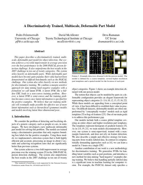
A Discriminatively Trained,Multiscale,Deformable Part ModelPedro Felzenszwalb University of Chicago pff@David McAllesterToyota Technological Institute at Chicagomcallester@Deva RamananUC Irvinedramanan@AbstractThis paper describes a discriminatively trained,multi-scale,deformable part model for object detection.Our sys-tem achieves a two-fold improvement in average precision over the best performance in the2006PASCAL person de-tection challenge.It also outperforms the best results in the 2007challenge in ten out of twenty categories.The system relies heavily on deformable parts.While deformable part models have become quite popular,their value had not been demonstrated on difficult benchmarks such as the PASCAL challenge.Our system also relies heavily on new methods for discriminative training.We combine a margin-sensitive approach for data mining hard negative examples with a formalism we call latent SVM.A latent SVM,like a hid-den CRF,leads to a non-convex training problem.How-ever,a latent SVM is semi-convex and the training prob-lem becomes convex once latent information is specified for the positive examples.We believe that our training meth-ods will eventually make possible the effective use of more latent information such as hierarchical(grammar)models and models involving latent three dimensional pose.1.IntroductionWe consider the problem of detecting and localizing ob-jects of a generic category,such as people or cars,in static images.We have developed a new multiscale deformable part model for solving this problem.The models are trained using a discriminative procedure that only requires bound-ing box labels for the positive ing these mod-els we implemented a detection system that is both highly efficient and accurate,processing an image in about2sec-onds and achieving recognition rates that are significantly better than previous systems.Our system achieves a two-fold improvement in average precision over the winning system[5]in the2006PASCAL person detection challenge.The system also outperforms the best results in the2007challenge in ten out of twenty This material is based upon work supported by the National Science Foundation under Grant No.0534820and0535174.Figure1.Example detection obtained with the person model.The model is defined by a coarse template,several higher resolution part templates and a spatial model for the location of each part. object categories.Figure1shows an example detection ob-tained with our person model.The notion that objects can be modeled by parts in a de-formable configuration provides an elegant framework for representing object categories[1–3,6,10,12,13,15,16,22]. While these models are appealing from a conceptual point of view,it has been difficult to establish their value in prac-tice.On difficult datasets,deformable models are often out-performed by“conceptually weaker”models such as rigid templates[5]or bag-of-features[23].One of our main goals is to address this performance gap.Our models include both a coarse global template cov-ering an entire object and higher resolution part templates. The templates represent histogram of gradient features[5]. As in[14,19,21],we train models discriminatively.How-ever,our system is semi-supervised,trained with a max-margin framework,and does not rely on feature detection. We also describe a simple and effective strategy for learn-ing parts from weakly-labeled data.In contrast to computa-tionally demanding approaches such as[4],we can learn a model in3hours on a single CPU.Another contribution of our work is a new methodology for discriminative training.We generalize SVMs for han-dling latent variables such as part positions,and introduce a new method for data mining“hard negative”examples dur-ing training.We believe that handling partially labeled data is a significant issue in machine learning for computer vi-sion.For example,the PASCAL dataset only specifies abounding box for each positive example of an object.We treat the position of each object part as a latent variable.We also treat the exact location of the object as a latent vari-able,requiring only that our classifier select a window that has large overlap with the labeled bounding box.A latent SVM,like a hidden CRF[19],leads to a non-convex training problem.However,unlike a hidden CRF, a latent SVM is semi-convex and the training problem be-comes convex once latent information is specified for thepositive training examples.This leads to a general coordi-nate descent algorithm for latent SVMs.System Overview Our system uses a scanning window approach.A model for an object consists of a global“root”filter and several part models.Each part model specifies a spatial model and a partfilter.The spatial model defines a set of allowed placements for a part relative to a detection window,and a deformation cost for each placement.The score of a detection window is the score of the root filter on the window plus the sum over parts,of the maxi-mum over placements of that part,of the partfilter score on the resulting subwindow minus the deformation cost.This is similar to classical part-based models[10,13].Both root and partfilters are scored by computing the dot product be-tween a set of weights and histogram of gradient(HOG) features within a window.The rootfilter is equivalent to a Dalal-Triggs model[5].The features for the partfilters are computed at twice the spatial resolution of the rootfilter. Our model is defined at afixed scale,and we detect objects by searching over an image pyramid.In training we are given a set of images annotated with bounding boxes around each instance of an object.We re-duce the detection problem to a binary classification prob-lem.Each example x is scored by a function of the form, fβ(x)=max zβ·Φ(x,z).Hereβis a vector of model pa-rameters and z are latent values(e.g.the part placements). To learn a model we define a generalization of SVMs that we call latent variable SVM(LSVM).An important prop-erty of LSVMs is that the training problem becomes convex if wefix the latent values for positive examples.This can be used in a coordinate descent algorithm.In practice we iteratively apply classical SVM training to triples( x1,z1,y1 ,..., x n,z n,y n )where z i is selected to be the best scoring latent label for x i under the model learned in the previous iteration.An initial rootfilter is generated from the bounding boxes in the PASCAL dataset. The parts are initialized from this rootfilter.2.ModelThe underlying building blocks for our models are the Histogram of Oriented Gradient(HOG)features from[5]. We represent HOG features at two different scales.Coarse features are captured by a rigid template covering anentireImage pyramidFigure2.The HOG feature pyramid and an object hypothesis de-fined in terms of a placement of the rootfilter(near the top of the pyramid)and the partfilters(near the bottom of the pyramid). detection window.Finer scale features are captured by part templates that can be moved with respect to the detection window.The spatial model for the part locations is equiv-alent to a star graph or1-fan[3]where the coarse template serves as a reference position.2.1.HOG RepresentationWe follow the construction in[5]to define a dense repre-sentation of an image at a particular resolution.The image isfirst divided into8x8non-overlapping pixel regions,or cells.For each cell we accumulate a1D histogram of gra-dient orientations over pixels in that cell.These histograms capture local shape properties but are also somewhat invari-ant to small deformations.The gradient at each pixel is discretized into one of nine orientation bins,and each pixel“votes”for the orientation of its gradient,with a strength that depends on the gradient magnitude.For color images,we compute the gradient of each color channel and pick the channel with highest gradi-ent magnitude at each pixel.Finally,the histogram of each cell is normalized with respect to the gradient energy in a neighborhood around it.We look at the four2×2blocks of cells that contain a particular cell and normalize the his-togram of the given cell with respect to the total energy in each of these blocks.This leads to a vector of length9×4 representing the local gradient information inside a cell.We define a HOG feature pyramid by computing HOG features of each level of a standard image pyramid(see Fig-ure2).Features at the top of this pyramid capture coarse gradients histogrammed over fairly large areas of the input image while features at the bottom of the pyramid capture finer gradients histogrammed over small areas.2.2.FiltersFilters are rectangular templates specifying weights for subwindows of a HOG pyramid.A w by hfilter F is a vector with w×h×9×4weights.The score of afilter is defined by taking the dot product of the weight vector and the features in a w×h subwindow of a HOG pyramid.The system in[5]uses a singlefilter to define an object model.That system detects objects from a particular class by scoring every w×h subwindow of a HOG pyramid and thresholding the scores.Let H be a HOG pyramid and p=(x,y,l)be a cell in the l-th level of the pyramid.Letφ(H,p,w,h)denote the vector obtained by concatenating the HOG features in the w×h subwindow of H with top-left corner at p.The score of F on this detection window is F·φ(H,p,w,h).Below we useφ(H,p)to denoteφ(H,p,w,h)when the dimensions are clear from context.2.3.Deformable PartsHere we consider models defined by a coarse rootfilter that covers the entire object and higher resolution partfilters covering smaller parts of the object.Figure2illustrates a placement of such a model in a HOG pyramid.The rootfil-ter location defines the detection window(the pixels inside the cells covered by thefilter).The partfilters are placed several levels down in the pyramid,so the HOG cells at that level have half the size of cells in the rootfilter level.We have found that using higher resolution features for defining partfilters is essential for obtaining high recogni-tion performance.With this approach the partfilters repre-sentfiner resolution edges that are localized to greater ac-curacy when compared to the edges represented in the root filter.For example,consider building a model for a face. The rootfilter could capture coarse resolution edges such as the face boundary while the partfilters could capture details such as eyes,nose and mouth.The model for an object with n parts is formally defined by a rootfilter F0and a set of part models(P1,...,P n) where P i=(F i,v i,s i,a i,b i).Here F i is afilter for the i-th part,v i is a two-dimensional vector specifying the center for a box of possible positions for part i relative to the root po-sition,s i gives the size of this box,while a i and b i are two-dimensional vectors specifying coefficients of a quadratic function measuring a score for each possible placement of the i-th part.Figure1illustrates a person model.A placement of a model in a HOG pyramid is given by z=(p0,...,p n),where p i=(x i,y i,l i)is the location of the rootfilter when i=0and the location of the i-th part when i>0.We assume the level of each part is such that a HOG cell at that level has half the size of a HOG cell at the root level.The score of a placement is given by the scores of eachfilter(the data term)plus a score of the placement of each part relative to the root(the spatial term), ni=0F i·φ(H,p i)+ni=1a i·(˜x i,˜y i)+b i·(˜x2i,˜y2i),(1)where(˜x i,˜y i)=((x i,y i)−2(x,y)+v i)/s i gives the lo-cation of the i-th part relative to the root location.Both˜x i and˜y i should be between−1and1.There is a large(exponential)number of placements for a model in a HOG pyramid.We use dynamic programming and distance transforms techniques[9,10]to compute the best location for the parts of a model as a function of the root location.This takes O(nk)time,where n is the number of parts in the model and k is the number of cells in the HOG pyramid.To detect objects in an image we score root locations according to the best possible placement of the parts and threshold this score.The score of a placement z can be expressed in terms of the dot product,β·ψ(H,z),between a vector of model parametersβand a vectorψ(H,z),β=(F0,...,F n,a1,b1...,a n,b n).ψ(H,z)=(φ(H,p0),φ(H,p1),...φ(H,p n),˜x1,˜y1,˜x21,˜y21,...,˜x n,˜y n,˜x2n,˜y2n,). We use this representation for learning the model parame-ters as it makes a connection between our deformable mod-els and linear classifiers.On interesting aspect of the spatial models defined here is that we allow for the coefficients(a i,b i)to be negative. This is more general than the quadratic“spring”cost that has been used in previous work.3.LearningThe PASCAL training data consists of a large set of im-ages with bounding boxes around each instance of an ob-ject.We reduce the problem of learning a deformable part model with this data to a binary classification problem.Let D=( x1,y1 ,..., x n,y n )be a set of labeled exam-ples where y i∈{−1,1}and x i specifies a HOG pyramid, H(x i),together with a range,Z(x i),of valid placements for the root and partfilters.We construct a positive exam-ple from each bounding box in the training set.For these ex-amples we define Z(x i)so the rootfilter must be placed to overlap the bounding box by at least50%.Negative exam-ples come from images that do not contain the target object. Each placement of the rootfilter in such an image yields a negative training example.Note that for the positive examples we treat both the part locations and the exact location of the rootfilter as latent variables.We have found that allowing uncertainty in the root location during training significantly improves the per-formance of the system(see Section4).tent SVMsA latent SVM is defined as follows.We assume that each example x is scored by a function of the form,fβ(x)=maxz∈Z(x)β·Φ(x,z),(2)whereβis a vector of model parameters and z is a set of latent values.For our deformable models we define Φ(x,z)=ψ(H(x),z)so thatβ·Φ(x,z)is the score of placing the model according to z.In analogy to classical SVMs we would like to trainβfrom labeled examples D=( x1,y1 ,..., x n,y n )by optimizing the following objective function,β∗(D)=argminβλ||β||2+ni=1max(0,1−y i fβ(x i)).(3)By restricting the latent domains Z(x i)to a single choice, fβbecomes linear inβ,and we obtain linear SVMs as a special case of latent tent SVMs are instances of the general class of energy-based models[18].3.2.Semi-ConvexityNote that fβ(x)as defined in(2)is a maximum of func-tions each of which is linear inβ.Hence fβ(x)is convex inβ.This implies that the hinge loss max(0,1−y i fβ(x i)) is convex inβwhen y i=−1.That is,the loss function is convex inβfor negative examples.We call this property of the loss function semi-convexity.Consider an LSVM where the latent domains Z(x i)for the positive examples are restricted to a single choice.The loss due to each positive example is now bined with the semi-convexity property,(3)becomes convex inβ.If the labels for the positive examples are notfixed we can compute a local optimum of(3)using a coordinate de-scent algorithm:1.Holdingβfixed,optimize the latent values for the pos-itive examples z i=argmax z∈Z(xi )β·Φ(x,z).2.Holding{z i}fixed for positive examples,optimizeβby solving the convex problem defined above.It can be shown that both steps always improve or maintain the value of the objective function in(3).If both steps main-tain the value we have a strong local optimum of(3),in the sense that Step1searches over an exponentially large space of latent labels for positive examples while Step2simulta-neously searches over weight vectors and an exponentially large space of latent labels for negative examples.3.3.Data Mining Hard NegativesIn object detection the vast majority of training exam-ples are negative.This makes it infeasible to consider all negative examples at a time.Instead,it is common to con-struct training data consisting of the positive instances and “hard negative”instances,where the hard negatives are data mined from the very large set of possible negative examples.Here we describe a general method for data mining ex-amples for SVMs and latent SVMs.The method iteratively solves subproblems using only hard instances.The innova-tion of our approach is a theoretical guarantee that it leads to the exact solution of the training problem defined using the complete training set.Our results require the use of a margin-sensitive definition of hard examples.The results described here apply both to classical SVMs and to the problem defined by Step2of the coordinate de-scent algorithm for latent SVMs.We omit the proofs of the theorems due to lack of space.These results are related to working set methods[17].We define the hard instances of D relative toβas,M(β,D)={ x,y ∈D|yfβ(x)≤1}.(4)That is,M(β,D)are training examples that are incorrectly classified or near the margin of the classifier defined byβ. We can show thatβ∗(D)only depends on hard instances. Theorem1.Let C be a subset of the examples in D.If M(β∗(D),D)⊆C thenβ∗(C)=β∗(D).This implies that in principle we could train a model us-ing a small set of examples.However,this set is defined in terms of the optimal modelβ∗(D).Given afixedβwe can use M(β,D)to approximate M(β∗(D),D).This suggests an iterative algorithm where we repeatedly compute a model from the hard instances de-fined by the model from the last iteration.This is further justified by the followingfixed-point theorem.Theorem2.Ifβ∗(M(β,D))=βthenβ=β∗(D).Let C be an initial“cache”of examples.In practice we can take the positive examples together with random nega-tive examples.Consider the following iterative algorithm: 1.Letβ:=β∗(C).2.Shrink C by letting C:=M(β,C).3.Grow C by adding examples from M(β,D)up to amemory limit L.Theorem3.If|C|<L after each iteration of Step2,the algorithm will converge toβ=β∗(D)infinite time.3.4.Implementation detailsMany of the ideas discussed here are only approximately implemented in our current system.In practice,when train-ing a latent SVM we iteratively apply classical SVM train-ing to triples x1,z1,y1 ,..., x n,z n,y n where z i is se-lected to be the best scoring latent label for x i under themodel trained in the previous iteration.Each of these triples leads to an example Φ(x i,z i),y i for training a linear clas-sifier.This allows us to use a highly optimized SVM pack-age(SVMLight[17]).On a single CPU,the entire training process takes3to4hours per object class in the PASCAL datasets,including initialization of the parts.Root Filter Initialization:For each category,we auto-matically select the dimensions of the rootfilter by looking at statistics of the bounding boxes in the training data.1We train an initial rootfilter F0using an SVM with no latent variables.The positive examples are constructed from the unoccluded training examples(as labeled in the PASCAL data).These examples are anisotropically scaled to the size and aspect ratio of thefilter.We use random subwindows from negative images to generate negative examples.Root Filter Update:Given the initial rootfilter trained as above,for each bounding box in the training set wefind the best-scoring placement for thefilter that significantly overlaps with the bounding box.We do this using the orig-inal,un-scaled images.We retrain F0with the new positive set and the original random negative set,iterating twice.Part Initialization:We employ a simple heuristic to ini-tialize six parts from the rootfilter trained above.First,we select an area a such that6a equals80%of the area of the rootfilter.We greedily select the rectangular region of area a from the rootfilter that has the most positive energy.We zero out the weights in this region and repeat until six parts are selected.The partfilters are initialized from the rootfil-ter values in the subwindow selected for the part,butfilled in to handle the higher spatial resolution of the part.The initial deformation costs measure the squared norm of a dis-placement with a i=(0,0)and b i=−(1,1).Model Update:To update a model we construct new training data triples.For each positive bounding box in the training data,we apply the existing detector at all positions and scales with at least a50%overlap with the given bound-ing box.Among these we select the highest scoring place-ment as the positive example corresponding to this training bounding box(Figure3).Negative examples are selected byfinding high scoring detections in images not containing the target object.We add negative examples to a cache un-til we encounterfile size limits.A new model is trained by running SVMLight on the positive and negative examples, each labeled with part placements.We update the model10 times using the cache scheme described above.In each it-eration we keep the hard instances from the previous cache and add as many new hard instances as possible within the memory limit.Toward thefinal iterations,we are able to include all hard instances,M(β,D),in the cache.1We picked a simple heuristic by cross-validating over5object classes. We set the model aspect to be the most common(mode)aspect in the data. We set the model size to be the largest size not larger than80%of thedata.Figure3.The image on the left shows the optimization of the la-tent variables for a positive example.The dotted box is the bound-ing box label provided in the PASCAL training set.The large solid box shows the placement of the detection window while the smaller solid boxes show the placements of the parts.The image on the right shows a hard-negative example.4.ResultsWe evaluated our system using the PASCAL VOC2006 and2007comp3challenge datasets and protocol.We refer to[7,8]for details,but emphasize that both challenges are widely acknowledged as difficult testbeds for object detec-tion.Each dataset contains several thousand images of real-world scenes.The datasets specify ground-truth bounding boxes for several object classes,and a detection is consid-ered correct when it overlaps more than50%with a ground-truth bounding box.One scores a system by the average precision(AP)of its precision-recall curve across a testset.Recent work in pedestrian detection has tended to report detection rates versus false positives per window,measured with cropped positive examples and negative images with-out objects of interest.These scores are tied to the reso-lution of the scanning window search and ignore effects of non-maximum suppression,making it difficult to compare different systems.We believe the PASCAL scoring method gives a more reliable measure of performance.The2007challenge has20object categories.We entered a preliminary version of our system in the official competi-tion,and obtained the best score in6categories.Our current system obtains the highest score in10categories,and the second highest score in6categories.Table1summarizes the results.Our system performs well on rigid objects such as cars and sofas as well as highly deformable objects such as per-sons and horses.We also note that our system is successful when given a large or small amount of training data.There are roughly4700positive training examples in the person category but only250in the sofa category.Figure4shows some of the models we learned.Figure5shows some ex-ample detections.We evaluated different components of our system on the longer-established2006person dataset.The top AP scoreaero bike bird boat bottle bus car cat chair cow table dog horse mbike person plant sheep sofa train tvOur rank 31211224111422112141Our score .180.411.092.098.249.349.396.110.155.165.110.062.301.337.267.140.141.156.206.336Darmstadt .301INRIA Normal .092.246.012.002.068.197.265.018.097.039.017.016.225.153.121.093.002.102.157.242INRIA Plus.136.287.041.025.077.279.294.132.106.127.067.071.335.249.092.072.011.092.242.275IRISA .281.318.026.097.119.289.227.221.175.253MPI Center .060.110.028.031.000.164.172.208.002.044.049.141.198.170.091.004.091.034.237.051MPI ESSOL.152.157.098.016.001.186.120.240.007.061.098.162.034.208.117.002.046.147.110.054Oxford .262.409.393.432.375.334TKK .186.078.043.072.002.116.184.050.028.100.086.126.186.135.061.019.036.058.067.090Table 1.PASCAL VOC 2007results.Average precision scores of our system and other systems that entered the competition [7].Empty boxes indicate that a method was not tested in the corresponding class.The best score in each class is shown in bold.Our current system ranks first in 10out of 20classes.A preliminary version of our system ranked first in 6classes in the official competition.BottleCarBicycleSofaFigure 4.Some models learned from the PASCAL VOC 2007dataset.We show the total energy in each orientation of the HOG cells in the root and part filters,with the part filters placed at the center of the allowable displacements.We also show the spatial model for each part,where bright values represent “cheap”placements,and dark values represent “expensive”placements.in the PASCAL competition was .16,obtained using a rigid template model of HOG features [5].The best previous re-sult of.19adds a segmentation-based verification step [20].Figure 6summarizes the performance of several models we trained.Our root-only model is equivalent to the model from [5]and it scores slightly higher at .18.Performance jumps to .24when the model is trained with a LSVM that selects a latent position and scale for each positive example.This suggests LSVMs are useful even for rigid templates because they allow for self-adjustment of the detection win-dow in the training examples.Adding deformable parts in-creases performance to .34AP —a factor of two above the best previous score.Finally,we trained a model with partsbut no root filter and obtained .29AP.This illustrates the advantage of using a multiscale representation.We also investigated the effect of the spatial model and allowable deformations on the 2006person dataset.Recall that s i is the allowable displacement of a part,measured in HOG cells.We trained a rigid model with high-resolution parts by setting s i to 0.This model outperforms the root-only system by .27to .24.If we increase the amount of allowable displacements without using a deformation cost,we start to approach a bag-of-features.Performance peaks at s i =1,suggesting it is useful to constrain the part dis-placements.The optimal strategy allows for larger displace-ments while using an explicit deformation cost.The follow-Figure 5.Some results from the PASCAL 2007dataset.Each row shows detections using a model for a specific class (Person,Bottle,Car,Sofa,Bicycle,Horse).The first three columns show correct detections while the last column shows false positives.Our system is able to detect objects over a wide range of scales (such as the cars)and poses (such as the horses).The system can also detect partially occluded objects such as a person behind a bush.Note how the false detections are often quite reasonable,for example detecting a bus with the car model,a bicycle sign with the bicycle model,or a dog with the horse model.In general the part filters represent meaningful object parts that are well localized in each detection such as the head in the person model.Figure6.Evaluation of our system on the PASCAL VOC2006 person dataset.Root uses only a rootfilter and no latent place-ment of the detection windows on positive examples.Root+Latent uses a rootfilter with latent placement of the detection windows. Parts+Latent is a part-based system with latent detection windows but no rootfilter.Root+Parts+Latent includes both root and part filters,and latent placement of the detection windows.ing table shows AP as a function of freely allowable defor-mation in thefirst three columns.The last column gives the performance when using a quadratic deformation cost and an allowable displacement of2HOG cells.s i01232+quadratic costAP.27.33.31.31.345.DiscussionWe introduced a general framework for training SVMs with latent structure.We used it to build a recognition sys-tem based on multiscale,deformable models.Experimental results on difficult benchmark data suggests our system is the current state-of-the-art in object detection.LSVMs allow for exploration of additional latent struc-ture for recognition.One can consider deeper part hierar-chies(parts with parts),mixture models(frontal vs.side cars),and three-dimensional pose.We would like to train and detect multiple classes together using a shared vocab-ulary of parts(perhaps visual words).We also plan to use A*search[11]to efficiently search over latent parameters during detection.References[1]Y.Amit and A.Trouve.POP:Patchwork of parts models forobject recognition.IJCV,75(2):267–282,November2007.[2]M.Burl,M.Weber,and P.Perona.A probabilistic approachto object recognition using local photometry and global ge-ometry.In ECCV,pages II:628–641,1998.[3] D.Crandall,P.Felzenszwalb,and D.Huttenlocher.Spatialpriors for part-based recognition using statistical models.In CVPR,pages10–17,2005.[4] D.Crandall and D.Huttenlocher.Weakly supervised learn-ing of part-based spatial models for visual object recognition.In ECCV,pages I:16–29,2006.[5]N.Dalal and B.Triggs.Histograms of oriented gradients forhuman detection.In CVPR,pages I:886–893,2005.[6] B.Epshtein and S.Ullman.Semantic hierarchies for recog-nizing objects and parts.In CVPR,2007.[7]M.Everingham,L.Van Gool,C.K.I.Williams,J.Winn,and A.Zisserman.The PASCAL Visual Object Classes Challenge2007(VOC2007)Results./challenges/VOC/voc2007/workshop.[8]M.Everingham, A.Zisserman, C.K.I.Williams,andL.Van Gool.The PASCAL Visual Object Classes Challenge2006(VOC2006)Results./challenges/VOC/voc2006/results.pdf.[9]P.Felzenszwalb and D.Huttenlocher.Distance transformsof sampled functions.Cornell Computing and Information Science Technical Report TR2004-1963,September2004.[10]P.Felzenszwalb and D.Huttenlocher.Pictorial structures forobject recognition.IJCV,61(1),2005.[11]P.Felzenszwalb and D.McAllester.The generalized A*ar-chitecture.JAIR,29:153–190,2007.[12]R.Fergus,P.Perona,and A.Zisserman.Object class recog-nition by unsupervised scale-invariant learning.In CVPR, 2003.[13]M.Fischler and R.Elschlager.The representation andmatching of pictorial structures.IEEE Transactions on Com-puter,22(1):67–92,January1973.[14] A.Holub and P.Perona.A discriminative framework formodelling object classes.In CVPR,pages I:664–671,2005.[15]S.Ioffe and D.Forsyth.Probabilistic methods forfindingpeople.IJCV,43(1):45–68,June2001.[16]Y.Jin and S.Geman.Context and hierarchy in a probabilisticimage model.In CVPR,pages II:2145–2152,2006.[17]T.Joachims.Making large-scale svm learning practical.InB.Sch¨o lkopf,C.Burges,and A.Smola,editors,Advances inKernel Methods-Support Vector Learning.MIT Press,1999.[18]Y.LeCun,S.Chopra,R.Hadsell,R.Marc’Aurelio,andF.Huang.A tutorial on energy-based learning.InG.Bakir,T.Hofman,B.Sch¨o lkopf,A.Smola,and B.Taskar,editors, Predicting Structured Data.MIT Press,2006.[19] A.Quattoni,S.Wang,L.Morency,M.Collins,and T.Dar-rell.Hidden conditional randomfields.PAMI,29(10):1848–1852,October2007.[20] ing segmentation to verify object hypothe-ses.In CVPR,pages1–8,2007.[21] D.Ramanan and C.Sminchisescu.Training deformablemodels for localization.In CVPR,pages I:206–213,2006.[22]H.Schneiderman and T.Kanade.Object detection using thestatistics of parts.IJCV,56(3):151–177,February2004. [23]J.Zhang,M.Marszalek,zebnik,and C.Schmid.Localfeatures and kernels for classification of texture and object categories:A comprehensive study.IJCV,73(2):213–238, June2007.。
英语科技术语的构词特点及其翻译

英语科技术语的构词特点及其翻译引言科技正在以惊人的速度发展,随之而来的是我们越来越依赖科技。
随着科技的普及,科技语言也越来越普及。
在技术领域,有各种各样的专业术语和术语,这些术语是该行业所特有的。
本文旨在探讨英语科技术语的构词特点及其翻译。
英语科技术语的构词特点前缀和后缀前缀和后缀在英语科技术语中常常被使用。
前缀添加在一个词的开头,而后缀添加在一个词的结尾。
常见的前缀包括“un-”,“re-”,“pre-”,“post-”,“multi-”,“mega-”,“micro-”,“nano-”,“tele-”等等。
常见的后缀包括“-logy”,“-graphy”,“-scope”,“-meter”,“-ology”,“-ics”,“-ism”,“-able”,“-ic”,“-ish”等等。
这些前缀和后缀可以帮助构建新的单词,并在其中加入新的含义。
例如,“multi-”前缀表示“多个”,“mega-”前缀表示“巨大的”,“micro-”前缀表示“微小的”,“nano-”前缀表示“纳米级别的”,这些前缀都是与尺寸相关的,它们可以与其他词结合使用,例如“multicore”(多核的),“megabyte”(兆字节),“microchip”(微芯片),“nanotechnology”(纳米技术)。
后缀“-logy”表示“学科”,“-graphy”表示“写作、制图”,“-scope”表示“观察仪器”,“-meter”表示“测量仪器”,“-ology”表示“学问”,“-ics”表示“学科、学说、体系”,“-ism”表示“主义、学说”,“-able”表示“能够”,“-ic”表示“有关的、性质的”,“-ish”表示“有点”的含义。
例如,“biology”(生物学),“photography”(摄影术),“microscope”(显微镜),“thermometer”(温度计),“geology”(地质学),“aesthetics”(美学),“communism”(共产主义),“compatible”(兼容的),“electronic”(电子的),“greenish”(稍微带绿色的)等。
常用量子化学词汇

Average,期望值,ab initio, 从头计算approximate,近似accurate, 精确atomiticity, 粒子性active, 活性的adiabatic, 绝热的,非常缓慢的anti-symmetry principle 反对称原理Basis,基组bra, 左矢,左矢空间,右矢空间的对偶空间boundary,边界条件Born-Oppenheimer 波恩奥本海默近似,绝热近似退耦后的进一步近似Configuration, 组态,电子排布correlation, 电子的相关作用commutation, 对易子coordinate, 坐标conjugate, 共轭core, 原子实convergence, 收敛,级数或积分收敛coupling, 耦合Coulomb’s Law, 库仑定律,麦克斯韦场方程的点电荷近似correspondence principle, 对应原理complete, 完备的complete active space (CAS), 完备的活性空间closed-shell, 闭壳层closed system, 封闭体系configuration state function (CSF)组态波函数Diagonalization,对角化Diagonal, 对角阵,对角元DFT, 密度泛函理论density,电子密度D-CI, double CIdynamical, 动力学的deterministic, 行列式的diabatic 未对角化的,非自身表象的,透热的Effective Hamiltonian, 有效哈密顿electron, 电子eigenvalue, 本征值eigenvector, 本征矢,无限维Hilbert空间中的态矢量external, 外加的energy, 能量excitation, 激发态excited, 被激发的exclusion principle不相容原理Functional, 泛函数function, 函数Fock space, Fock空间force, 力.,field场Gradient,梯度Gaussian, 高斯程序,高斯函数generic, 普适的Gauge 规范Hamiltonian, 哈密顿,Hessian, 二阶导数Hermitian, 厄米的Hartree 原子能量单位Integral, 积分internal, 内部的(内部自由度的)interaction, 相互作用independent, 不独立的invariant, 不变的iteration, 叠代interpretation, (几率)诠释interpolation,inactive不活动的J-integral, j积分jj-coupling jj耦合K-integral, k积分ket,右矢,右矢空间Linear algebra, 线性代数,linear combination of atomic orbitals (LCAO),原子轨函线性组合(法)local, 定域的locality, 定域物理量linear scaling, 线性标度low order,低对称性,有序度较低的情形Matrix, 矩阵,metric,矩阵的momentum, momenta,动量many-body theory,多体理论mechanics,力学,机理,机制multiconfiguration self-consistent field (MCSCF),多组态自洽场multireference (MR),多参考态方法minimization,最小化Normalization,归一化normal order, 正常序norm,已归一化的(波函数),N-electron, N电子体系nondynamic,非动力学的nonadiabtaic 非绝热的,有交换作用的,非渐变的Orbit,轨道orbital,轨道波函数,轨函observable, 可观测的(物理量)operator, 算符optimization, 优化one-electron,单电子,orthogonal, 正交的orthonormal, 正交归一的,open-shell,开壳层open system,开放体系,order-N第N阶(近似,导数)Principle,原理,原则property,性质particle, 粒子probability, 几率probabilistic, 几率性的potential,势PES, 势能面pseudo-, 赝的,pseudo vector赝矢量,pseudopotential,赝势perturbation theory,微扰理论Quantum, quanta, 量子quantized, 使量子化quantization,量子化的过程quotient,商quantity,数量,物理量Relativity,相对论,relativistic, 相对论性的representation,表示,表象Reference,参考系,参考态Spin, 自旋S-matrix, s矩阵,线性变换矩阵,散射矩阵symmetry, 对称性SCF, 自洽场stability,稳定性state,态scale,标度,测量shell,电子壳层spin-orbit coupling,自旋轨道耦合static,静态的space,空间,坐标空间的,banach/Hilbert Space,巴拉赫,希尔伯特空间spatial,空间的similarity transformation, 相似变换self-consistent field (SCF), 自洽场secondary ,二阶的,二级的,second quantization,二次量子化Transition state,过渡态time-dependent,含时的,对时间依赖的trace,矩阵的迹.Transformation,变换Universal,统一的,全同的。
凝聚态物理材料物理专业考博量子物理领域英文高频词汇
凝聚态物理材料物理专业考博量子物理领域英文高频词汇1. Quantum Mechanics - 量子力学2. Wavefunction - 波函数3. Hamiltonian - 哈密顿量4. Schrödinger Equation - 薛定谔方程5. Quantum Field Theory - 量子场论6. Quantum Entanglement - 量子纠缠7. Uncertainty Principle - 不确定性原理8. Quantum Tunneling - 量子隧穿9. Quantum Superposition - 量子叠加10. Quantum Decoherence - 量子退相干11. Spin - 自旋12. Quantum Computing - 量子计算13. Quantum Teleportation - 量子纠缠传输14. Quantum Interference - 量子干涉15. Quantum Information - 量子信息16. Quantum Optics - 量子光学17. Quantum Dots - 量子点18. Quantum Hall Effect - 量子霍尔效应19. Bose-Einstein Condensate - 玻色-爱因斯坦凝聚态20. Fermi-Dirac Statistics - 费米-狄拉克统计中文翻译:1. Quantum Mechanics - 量子力学2. Wavefunction - 波函数3. Hamiltonian - 哈密顿量4. Schrödinger Equation - 薛定谔方程5. Quantum Field Theory - 量子场论6. Quantum Entanglement - 量子纠缠7. Uncertainty Principle - 不确定性原理8. Quantum Tunneling - 量子隧穿9. Quantum Superposition - 量子叠加10. Quantum Decoherence - 量子退相干11. Spin - 自旋12. Quantum Computing - 量子计算13. Quantum Teleportation - 量子纠缠传输14. Quantum Interference - 量子干涉15. Quantum Information - 量子信息16. Quantum Optics - 量子光学17. Quantum Dots - 量子点18. Quantum Hall Effect - 量子霍尔效应19. Bose-Einstein Condensate - 玻色-爱因斯坦凝聚态20. Fermi-Dirac Statistics - 费米-狄拉克统计。