ARTICLE NO. GE985251 Performance-Guarantee Gene Predictions via Spliced Alignment
A File is Not a File
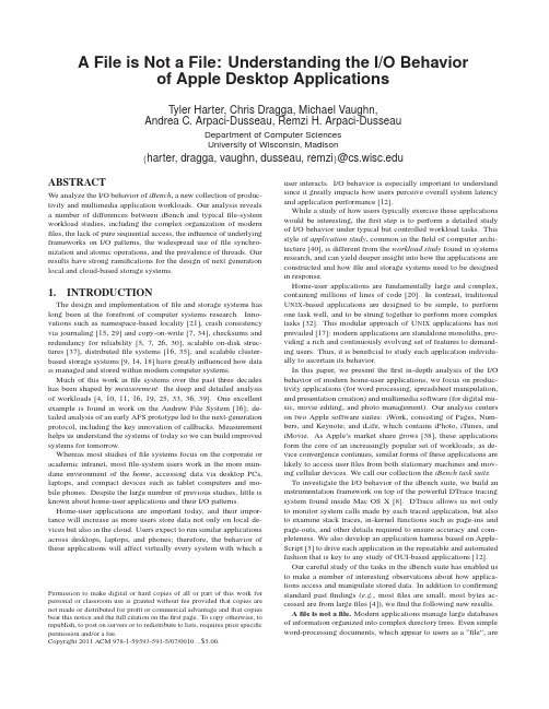
A File is Not a File:Understanding the I/O Behaviorof Apple Desktop ApplicationsTyler Harter,Chris Dragga,Michael Vaughn,Andrea C.Arpaci-Dusseau,Remzi H.Arpaci-DusseauDepartment of Computer SciencesUniversity of Wisconsin,Madison{harter,dragga,vaughn,dusseau,remzi}@ABSTRACTWe analyze the I/O behavior of iBench,a new collection of produc-tivity and multimedia application workloads.Our analysis reveals a number of differences between iBench and typicalfile-system workload studies,including the complex organization of modern files,the lack of pure sequential access,the influence of underlying frameworks on I/O patterns,the widespread use offile synchro-nization and atomic operations,and the prevalence of threads.Our results have strong ramifications for the design of next generation local and cloud-based storage systems.1.INTRODUCTIONThe design and implementation offile and storage systems has long been at the forefront of computer systems research.Inno-vations such as namespace-based locality[21],crash consistency via journaling[15,29]and copy-on-write[7,34],checksums and redundancy for reliability[5,7,26,30],scalable on-disk struc-tures[37],distributedfile systems[16,35],and scalable cluster-based storage systems[9,14,18]have greatly influenced how data is managed and stored within modern computer systems.Much of this work infile systems over the past three decades has been shaped by measurement:the deep and detailed analysis of workloads[4,10,11,16,19,25,33,36,39].One excellent example is found in work on the Andrew File System[16];de-tailed analysis of an early AFS prototype led to the next-generation protocol,including the key innovation of callbacks.Measurement helps us understand the systems of today so we can build improved systems for tomorrow.Whereas most studies offile systems focus on the corporate or academic intranet,mostfile-system users work in the more mun-dane environment of the home,accessing data via desktop PCs, laptops,and compact devices such as tablet computers and mo-bile phones.Despite the large number of previous studies,little is known about home-user applications and their I/O patterns. Home-user applications are important today,and their impor-tance will increase as more users store data not only on local de-vices but also in the ers expect to run similar applications across desktops,laptops,and phones;therefore,the behavior of these applications will affect virtually every system with which a Permission to make digital or hard copies of all or part of this work for personal or classroom use is granted without fee provided that copies are not made or distributed for profit or commercial advantage and that copies bear this notice and the full citation on thefirst page.To copy otherwise,to republish,to post on servers or to redistribute to lists,requires prior specific permission and/or a fee.Copyright2011ACM978-1-59593-591-5/07/0010...$er interacts.I/O behavior is especially important to understand since it greatly impacts how users perceive overall system latency and application performance[12].While a study of how users typically exercise these applications would be interesting,thefirst step is to perform a detailed study of I/O behavior under typical but controlled workload tasks.This style of application study,common in thefield of computer archi-tecture[40],is different from the workload study found in systems research,and can yield deeper insight into how the applications are constructed and howfile and storage systems need to be designed in response.Home-user applications are fundamentally large and complex, containing millions of lines of code[20].In contrast,traditional U NIX-based applications are designed to be simple,to perform one task well,and to be strung together to perform more complex tasks[32].This modular approach of U NIX applications has not prevailed[17]:modern applications are standalone monoliths,pro-viding a rich and continuously evolving set of features to demand-ing users.Thus,it is beneficial to study each application individu-ally to ascertain its behavior.In this paper,we present thefirst in-depth analysis of the I/O behavior of modern home-user applications;we focus on produc-tivity applications(for word processing,spreadsheet manipulation, and presentation creation)and multimedia software(for digital mu-sic,movie editing,and photo management).Our analysis centers on two Apple software suites:iWork,consisting of Pages,Num-bers,and Keynote;and iLife,which contains iPhoto,iTunes,and iMovie.As Apple’s market share grows[38],these applications form the core of an increasingly popular set of workloads;as de-vice convergence continues,similar forms of these applications are likely to access userfiles from both stationary machines and mov-ing cellular devices.We call our collection the iBench task suite. To investigate the I/O behavior of the iBench suite,we build an instrumentation framework on top of the powerful DTrace tracing system found inside Mac OS X[8].DTrace allows us not only to monitor system calls made by each traced application,but also to examine stack traces,in-kernel functions such as page-ins and page-outs,and other details required to ensure accuracy and com-pleteness.We also develop an application harness based on Apple-Script[3]to drive each application in the repeatable and automated fashion that is key to any study of GUI-based applications[12]. Our careful study of the tasks in the iBench suite has enabled us to make a number of interesting observations about how applica-tions access and manipulate stored data.In addition to confirming standard pastfindings(e.g.,mostfiles are small;most bytes ac-cessed are from largefiles[4]),wefind the following new results. Afile is not afile.Modern applications manage large databases of information organized into complex directory trees.Even simple word-processing documents,which appear to users as a“file”,arein actuality smallfile systems containing many sub-files(e.g.,a Microsoft.docfile is actually a FATfile system containing pieces of the document).File systems should be cognizant of such hidden structure in order to lay out and access data in these complexfiles more effectively.Sequential access is not sequential.Building on the trend no-ticed by V ogels for Windows NT[39],we observe that even for streaming media workloads,“pure”sequential access is increas-ingly rare.Sincefile formats often include metadata in headers, applications often read and re-read thefirst portion of afile before streaming through its contents.Prefetching and other optimizations might benefit from a deeper knowledge of thesefile formats. Auxiliaryfiles dominate.Applications help users create,mod-ify,and organize content,but userfiles represent a small fraction of thefiles touched by modern applications.Mostfiles are helper files that applications use to provide a rich graphical experience, support multiple languages,and record history and other metadata. File-system placement strategies might reduce seeks by grouping the hundreds of helperfiles used by an individual application. Writes are often forced.As the importance of home data in-creases(e.g.,family photos),applications are less willing to simply write data and hope it is eventuallyflushed to disk.Wefind that most written data is explicitly forced to disk by the application;for example,iPhoto calls fsync thousands of times in even the sim-plest of tasks.Forfile systems and storage,the days of delayed writes[22]may be over;new ideas are needed to support applica-tions that desire durability.Renaming is popular.Home-user applications commonly use atomic operations,in particular rename,to present a consistent view offiles to users.Forfile systems,this may mean that trans-actional capabilities[23]are needed.It may also necessitate a re-thinking of traditional means offile locality;for example,placing afile on disk based on its parent directory[21]does not work as expected when thefile isfirst created in a temporary location and then renamed.Multiple threads perform I/O.Virtually all of the applications we study issue I/O requests from a number of threads;a few ap-plications launch I/Os from hundreds of threads.Part of this us-age stems from the GUI-based nature of these applications;it is well known that threads are required to perform long-latency oper-ations in the background to keep the GUI responsive[24].Thus,file and storage systems should be thread-aware so they can better allocate bandwidth.Frameworks influence I/O.Modern applications are often de-veloped in sophisticated IDEs and leverage powerful libraries,such as Cocoa and Carbon.Whereas UNIX-style applications often di-rectly invoke system calls to read and writefiles,modern libraries put more code between applications and the underlyingfile system; for example,including"cocoa.h"in a Mac application imports 112,047lines of code from689differentfiles[28].Thus,the be-havior of the framework,and not just the application,determines I/O patterns.Wefind that the default behavior of some Cocoa APIs induces extra I/O and possibly unnecessary(and costly)synchro-nizations to disk.In addition,use of different libraries for similar tasks within an application can lead to inconsistent behavior be-tween those tasks.Future storage design should take these libraries and frameworks into account.This paper contains four major contributions.First,we describe a general tracing framework for creating benchmarks based on in-teractive tasks that home users may perform(e.g.,importing songs, exporting video clips,saving documents).Second,we deconstruct the I/O behavior of the tasks in iBench;we quantify the I/O behav-ior of each task in numerous ways,including the types offiles ac-cessed(e.g.,counts and sizes),the access patterns(e.g.,read/write, sequentiality,and preallocation),transactional properties(e.g.,dura-bility and atomicity),and threading.Third,we describe how these qualitative changes in I/O behavior may impact the design of future systems.Finally,we present the34traces from the iBench task suite;by making these traces publicly available and easy to use,we hope to improve the design,implementation,and evaluation of the next generation of local and cloud storage systems:/adsl/Traces/ibench The remainder of this paper is organized as follows.We begin by presenting a detailed timeline of the I/O operations performed by one task in the iBench suite;this motivates the need for a systematic study of home-user applications.We next describe our methodol-ogy for creating the iBench task suite.We then spend the majority of the paper quantitatively analyzing the I/O characteristics of the full iBench suite.Finally,we summarize the implications of our findings onfile-system design.2.CASE STUDYThe I/O characteristics of modern home-user applications are distinct from those of U NIX applications studied in the past.To motivate the need for a new study,we investigate the complex I/O behavior of a single representative task.Specifically,we report in detail the I/O performed over time by the Pages(4.0.3)application, a word processor,running on Mac OS X Snow Leopard(10.6.2)as it creates a blank document,inserts15JPEG images each of size 2.5MB,and saves the document as a Microsoft.docfile.Figure1shows the I/O this task performs(see the caption for a description of the symbols used).The top portion of thefigure il-lustrates the accesses performed over the full lifetime of the task:at a high level,it shows that more than385files spanning six different categories are accessed by eleven different threads,with many in-tervening calls to fsync and rename.The bottom portion of the figure magnifies a short time interval,showing the reads and writes performed by a single thread accessing the primary.doc productiv-ityfile.From this one experiment,we illustrate eachfinding de-scribed in the introduction.Wefirst focus on the single access that saves the user’s document(bottom),and then consider the broader context surrounding thisfile save,where we observe aflurry of ac-cesses to hundreds of helperfiles(top).Afile is not afile.Focusing on the magnified timeline of reads and writes to the productivity.docfile,we see that thefile format comprises more than just a simplefile.Microsoft.docfiles are based on the FATfile system and allow bundling of multiplefiles in the single.docfile.This.docfile contains a directory(Root),three streams for large data(WordDocument,Data,and1Table),and a stream for small data(Ministream).Space is allocated in thefile with three sections:afile allocation table(FAT),a double-indirect FAT(DIF)region,and a ministream allocation region(Mini). Sequential access is not sequential.The complex FAT-based file format causes random access patterns in several ways:first,the header is updated at the beginning and end of the magnified access; second,data from individual streams is fragmented throughout the file;and third,the1Table stream is updated before and after each image is appended to the WordDocument stream.Auxiliaryfiles dominate.Although saving the single.doc we have been considering is the sole purpose of this task,we now turn our attention to the top timeline and see that385differentfiles are accessed.There are several reasons for this multitude offiles. First,Pages provides a rich graphical experience involving many images and other forms of multimedia;together with the15in-serted JPEGs,this requires118multimediafiles.Second,usersF i l e sSequential RunsF i l e O f f s e t (K B )Figure 1:Pages Saving A Word Document.The top graph shows the 75-second timeline of the entire run,while the bottom graph is a magnified view of seconds 54to 58.In the top graph,annotations on the left categorize files by type and indicate file count and amount of I/O;annotations on the right show threads.Black bars are file accesses (reads and writes),with thickness logarithmically proportional to bytes of I/O./is an fsync ;\is a rename ;X is both.In the bottom graph,individual reads and writes to the .doc file are shown.Vertical bar position and bar length represent the offset within the file and number of bytes touched.Thick white bars are reads;thin gray bars are writes.Repeated runs are marked with the number of repetitions.Annotations on the right indicate the name of each file section.want to use Pages in their native language,so application text is not hard-coded into the executable but is instead stored in25different .stringsfiles.Third,to save user preferences and other metadata, Pages uses a SQLite database(2files)and a number of key-value stores(218.plistfiles).Writes are often forced;renaming is popular.Pages uses both of these actions to enforce basic transactional guarantees.It uses fsync toflush write data to disk,making it durable;it uses rename to atomically replace oldfiles with newfiles so that afile never contains inconsistent data.The timeline shows these invo-cations numerous times.First,Pages regularly uses fsync and rename when updating the key-value store of a.plistfile.Second, fsync is used on the SQLite database.Third,for each of the15 image insertions,Pages calls fsync on afile named“tempData”(classified as“other”)to update its automatic backup.Multiple threads perform I/O.Pages is a multi-threaded appli-cation and issues I/O requests from many different threads during the ing multiple threads for I/O allows Pages to avoid blocking while I/O requests are outstanding.Examining the I/O behavior across threads,we see that Thread1performs the most significant portion of I/O,but ten other threads are also involved.In most cases,a single thread exclusively accesses afile,but it is not uncommon for multiple threads to share afile.Frameworks influence I/O.Pages was developed in a rich pro-gramming environment where frameworks such as Cocoa or Car-bon are used for I/O;these libraries impact I/O patterns in ways the developer might not expect.For example,although the appli-cation developers did not bother to use fsync or rename when saving the user’s work in the.docfile,the Cocoa library regularly uses these calls to atomically and durably update relatively unim-portant metadata,such as“recently opened”lists stored in.plist files.As another example,when Pages tries to read data in512-byte chunks from the.doc,each read goes through the STDIO library, which only reads in4KB chunks.Thus,when Pages attempts to read one chunk from the1Table stream,seven unrequested chunks from the WordDocument stream are also incidentally read(off-set12039KB).In other cases,regions of the.docfile are repeat-edly accessed unnecessarily.For example,around the3KB off-set,read/write pairs occur dozens of times.Pages uses a library to write2-byte words;each time a word is written,the library reads, updates,and writes back an entire512-byte chunk.Finally,we see evidence of redundancy between libraries:even though Pages has a backing SQLite database for some of its properties,it also uses.plistfiles,which function across Apple applications as generic property stores.This one detailed experiment has shed light on a number of in-teresting I/O behaviors that indicate that home-user applications are indeed different than traditional workloads.A new workload suite is needed that more accurately reflects these applications.3.IBENCH TASK SUITEOur goal in constructing the iBench task suite is two-fold.First, we would like iBench to be representative of the tasks performed by home users.For this reason,iBench contains popular applications from the iLife and iWork suites for entertainment and productivity. Second,we would like iBench to be relatively simple for others to use forfile and storage system analysis.For this reason,we auto-mate the interactions of a home user and collect the resulting traces of I/O system calls.The traces are available online at this site: /adsl/Traces/ibench.We now describe in more detail how we met these two goals.3.1RepresentativeTo capture the I/O behavior of home users,iBench models the ac-tions of a“reasonable”user interacting with iPhoto,iTunes,iMovie, Pages,Numbers,and Keynote.Since the research community does not yet have data on the exact distribution of tasks that home users perform,iBench contains tasks that we believe are common and usesfiles with sizes that can be justified for a reasonable user. iBench contains34different tasks,each representing a home user performing one distinct operation.If desired,these tasks could be combined to create more complex workflows and I/O workloads. The six applications and corresponding tasks are as follows.iLife iPhoto8.1.1(419):digital photo album and photo manip-ulation software.iPhoto stores photos in a library that contains the data for the photos(which can be in a variety of formats,including JPG,TIFF,and PNG),a directory of modifiedfiles,a directory of scaled down images,and twofiles of thumbnail images.The library stores metadata in a SQLite database.iBench contains six tasks ex-ercising user actions typical for iPhoto:starting the application and importing,duplicating,editing,viewing,and deleting photos in the library.These tasks modify both the imagefiles and the underlying database.Each of the iPhoto tasks operates on4002.5MB photos, representing a user who has imported12megapixel photos(2.5MB each)from a full1GBflash card on his or her camera.iLife iTunes9.0.3(15):a media player capable of both audio and video playback.iTunes organizes itsfiles in a private library and supports most common music formats(e.g.,MP3,AIFF,W A VE, AAC,and MPEG-4).iTunes does not employ a database,keeping media metadata and playlists in both a binary and an XMLfile. iBench containsfive tasks for iTunes:starting iTunes,importing and playing an album of MP3songs,and importing and playing an MPEG-4movie.Importing requires copyingfiles into the library directory and,for music,analyzing each songfile for gapless play-back.The music tasks operate over an album(or playlist)of ten songs while the movie tasks use a single3-minute movie.iLife iMovie8.0.5(820):video editing software.iMovie stores its data in a library that contains directories for raw footage and projects,andfiles containing video footage thumbnails.iMovie supports both MPEG-4and Quicktimefiles.iBench contains four tasks for iMovie:starting iMovie,importing an MPEG-4movie, adding a clip from this movie into a project,and exporting a project to MPEG-4.The tasks all use a3-minute movie because this is a typical length found from home users on video-sharing websites. iWork Pages4.0.3(766):a word processor.Pages uses a ZIP-basedfile format and can export to DOC,PDF,RTF,and basic text. iBench includes eight tasks for Pages:starting up,creating and saving,opening,and exporting documents with and without images and with different formats.The tasks use15page documents. iWork Numbers2.0.3(332):a spreadsheet application.Num-bers organizes itsfiles with a ZIP-based format and exports to XLS and PDF.The four iBench tasks for Numbers include starting Num-bers,generating a spreadsheet and saving it,opening the spread-sheet,and exporting that spreadsheet to XLS.To model a possible home user working on a budget,the tasks utilize afive page spread-sheet with one column graph per sheet.iWork Keynote5.0.3(791):a presentation and slideshow appli-cation.Keynote saves to a.key ZIP-based format and exports to Microsoft’s PPT format.The seven iBench tasks for Keynote in-clude starting Keynote,creating slides with and without images, opening and playing presentations,and exporting to PPT.Each Keynote task uses a20-slide presentation.Accesses I/O MB Name DescriptionFiles (MB)Accesses (MB)RD%WR%/CPU Sec/CPU Seci L i f e i P h o t oStart Open iPhoto with library of 400photos 779(336.7)828(25.4)78.821.2151.1 4.6Imp Import 400photos into empty library 5900(1966.9)8709(3940.3)74.425.626.712.1Dup Duplicate 400photos from library2928(1963.9)5736(2076.2)52.447.6237.986.1Edit Sequentially edit 400photos from library 12119(4646.7)18927(12182.9)69.830.219.612.6Del Sequentially delete 400photos;empty trash 15246(23.0)15247(25.0)21.878.2280.90.5View Sequentially view 400photos 2929(1006.4)3347(1005.0)98.1 1.924.17.2i T u n e s Start Open iTunes with 10song album 143(184.4)195(9.3)54.745.372.4 3.4ImpS Import 10song album to library 68(204.9)139(264.5)66.333.775.2143.1ImpM Import 3minute movie to library 41(67.4)57(42.9)48.052.0152.4114.6PlayS Play album of 10songs 61(103.6)80(90.9)96.9 3.10.40.5PlayM Play 3minute movie56(77.9)69(32.0)92.37.7 2.2 1.0i M o v i e Start Open iMovie with 3minute clip in project 433(223.3)786(29.4)99.90.1134.8 5.0Imp Import 3minute .m4v (20MB)to “Events”184(440.1)383(122.3)55.644.429.39.3Add Paste 3minute clip from “Events”to project 210(58.3)547(2.2)47.852.2357.8 1.4Exp Export 3minute video clip 70(157.9)546(229.9)55.144.9 2.3 1.0i W o r kP a g e s Start Open Pages218(183.7)228(2.3)99.90.197.7 1.0New Create 15text page document;save as .pages 135(1.6)157(1.0)73.326.750.80.3NewP Create 15JPG document;save as .pages 408(112.0)997(180.9)60.739.354.69.9Open Open 15text page document 103(0.8)109(0.6)99.50.557.60.3PDF Export 15page document as .pdf 107(1.5)115(0.9)91.09.041.30.3PDFP Export 15JPG document as .pdf 404(77.4)965(110.9)67.432.649.7 5.7DOC Export 15page document as .doc 112(1.0)121(1.0)87.912.144.40.4DOCP Export 15JPG document as .doc 385(111.3)952(183.8)61.138.946.38.9N u m b e r s Start Open Numbers283(179.9)360(2.6)99.60.4115.50.8New Save 5sheets/column graphs as .numbers 269(4.9)313(2.8)90.79.39.60.1Open Open 5sheet spreadsheet119(1.3)137(1.3)99.80.248.70.5XLS Export 5sheets/column graphs as .xls 236(4.6)272(2.7)94.9 5.18.50.1K e y n o t e Start Open Keynote517(183.0)681(1.1)99.80.2229.80.4New Create 20text slides;save as .key 637(12.1)863(5.4)92.47.6129.10.8NewP Create 20JPG slides;save as .key654(92.9)901(103.3)66.833.270.88.1Play Open and play presentation of 20text slides 318(11.5)385(4.9)99.80.295.0 1.2PlayP Open and play presentation of 20JPG slides 321(45.4)388(55.7)69.630.472.410.4PPT Export 20text slides as .ppt 685(12.8)918(10.1)78.821.2115.2 1.3PPTP Export 20JPG slides as .ppt 723(110.6)996(124.6)57.642.461.07.6Table 1:34Tasks of the iBench Suite.The table summarizes the 34tasks of iBench,specifying the application,a short name for the task,and a longer description of the actions modeled.The I/O is characterized according to the number of files read or written,the sum of the maximum sizes of all accessed files,the number of file accesses that read or write data,the number of bytes read or written,the percentage of I/O bytes that are part of a read (or write),and the rate of I/O per CPU-second in terms of both file accesses and bytes.Each core is counted individually,so at most 2CPU-seconds can be counted per second on our dual-core test machine.CPU utilization is measured with the UNIX top utility,which in rare cases produces anomalous CPU utilization snapshots;those values are ignored.Table 1contains a brief description of each of the 34iBench tasks as well as the basic I/O characteristics of each task when running on Mac OS X Snow Leopard 10.6.2.The table illustrates that the iBench tasks perform a significant amount of I/O.Most tasks access hundreds of files,which in aggregate contain tens or hundreds of megabytes of data.The tasks typically access files hundreds of times.The tasks perform widely differing amounts of I/O,from less than a megabyte to more than a gigabyte.Most of the tasks perform many more reads than writes.Finally,the tasks exhibit high I/O throughput,often transferring tens of megabytes of data for every second of computation.3.2Easy to UseTo enable other system evaluators to easily use these tasks,the iBench suite is packaged as a set of 34system call traces.To ensure reproducible results,the 34user tasks were first automated with AppleScript,a general-purpose GUI scripting language.Apple-Script provides generic commands to emulate mouse clicks through menus and application-specific commands to capture higher-level operations.Application-specific commands bypass a small amount of I/O by skipping dialog boxes;however,we use them whenever possible for expediency.The system call traces were gathered using DTrace [8],a kernel and user level dynamic instrumentation tool.DTrace is used toinstrument the entry and exit points of all system calls dealing with the file system;it also records the current state of the system and the parameters passed to and returned from each call.While tracing with DTrace was generally straightforward,we ad-dressed four challenges in collecting the iBench traces.First,file sizes are not always available to DTrace;thus,we record every file’s initial size and compute subsequent file size changes caused by system calls such as write or ftruncate .Second,iTunes uses the ptrace system call to disable tracing;we circumvent this block by using gdb to insert a breakpoint that automatically re-turns without calling ptrace .Third,the volfs pseudo-file sys-tem in HFS+(Hierarchical File System)allows files to be opened via their inode number instead of a file name;to include path-names in the trace,we instrument the build path function to obtain the full path when the task is run.Fourth,tracing system calls misses I/O resulting from memory-mapped files;therefore,we purged memory and instrumented kernel page-in functions to measure the amount of memory-mapped file activity.We found that the amount of memory-mapped I/O is negligible in most tasks;we thus do not include this I/O in the iBench traces or analysis.To provide reproducible results,the traces must be run on a sin-gle file-system image.Therefore,the iBench suite also contains snapshots of the initial directories to be restored before each run;initial state is critical in file-system benchmarking [1].4.ANALYSIS OF IBENCH TASKSThe iBench task suite enables us to study the I/O behavior of a large set of home-user actions.As shown from the timeline of I/O behavior for one particular task in Section2,these tasks are likely to accessfiles in complex ways.To characterize this complex behavior in a quantitative manner across the entire suite of34tasks, we focus on answering four categories of questions.•What different types offiles are accessed and what are the sizes of thesefiles?•How arefiles accessed for reads and writes?Arefiles ac-cessed sequentially?Is space preallocated?•What are the transactional properties?Are writesflushed with fsync or performed atomically?•How do multi-threaded applications distribute I/O across dif-ferent threads?Answering these questions has two benefits.First,the answers can guidefile and storage system developers to target their systems better to home-user applications.Second,the characterization will help users of iBench to select the most appropriate traces for eval-uation and to understand their resulting behavior.All measurements were performed on a Mac Mini running Mac OS X Snow Leopard version10.6.2and the HFS+file system. The machine has2GB of memory and a2.26GHz Intel Core Duo processor.4.1Nature of FilesOur analysis begins by characterizing the high-level behavior of the iBench tasks.In particular,we study the different types offiles opened by each iBench task as well as the sizes of thosefiles. 4.1.1File TypesThe iLife and iWork applications store data across a variety of files in a number of different formats;for example,iLife applica-tions tend to store their data in libraries(or data directories)unique to each user,while iWork applications organize their documents in proprietary ZIP-basedfiles.The extent to which tasks access dif-ferent types offiles greatly influences their I/O behavior.To understand accesses to differentfile types,we place eachfile into one of six categories,based onfile name extensions and us-age.Multimediafiles contain images(e.g.,JPEG),songs(e.g., MP3,AIFF),and movies(e.g.,MPEG-4).Productivityfiles are documents(e.g.,.pages,DOC,PDF),spreadsheets(e.g.,.numbers, XLS),and presentations(e.g.,.key,PPT).SQLitefiles are database files.Plistfiles are property-listfiles in XML containing key-value pairs for user preferences and application properties.Stringsfiles contain strings for localization of application text.Finally,Other contains miscellaneousfiles such as plain text,logs,files without extensions,and binaryfiles.Figure2shows the frequencies with which tasks open and ac-cessfiles of each type;most tasks perform hundreds of these ac-cesses.Multimediafile opens are common in all workloads,though they seldom predominate,even in the multimedia-heavy iLife ap-plications.Conversely,opens of productivityfiles are rare,even in iWork applications that use them;this is likely because most iWork tasks create or view a single productivityfile.Because.plistfiles act as generic helperfiles,they are relatively common.SQLitefiles only have a noticeable presence in iPhoto,where they account for a substantial portion of the observed opens.Stringsfiles occupy a significant minority of most workloads(except iPhoto and iTunes). Finally,between5%and20%offiles are of type“Other”(except for iTunes,where they are more prevalent).Figure3displays the percentage of I/O bytes accessed for each file type.In bytes,multimedia I/O dominates most of the iLife tasks,while productivity I/O has a significant presence in the iWork tasks;file descriptors on multimedia and productivityfiles tend to receive large amounts of I/O.SQLite,Plist,and Stringsfiles have a smaller share of the total I/O in bytes relative to the number of openedfiles;this implies that tasks access only a small quantity of data for each of thesefiles opened(e.g.,several key-value pairs in a.plist).In most tasks,files classified as“Other”receive a more significant portion of the I/O(the exception is iTunes). Summary:Home applications access a wide variety offile types, generally opening multimediafiles the most frequently.iLife tasks tend to access bytes primarily from multimedia orfiles classified as“Other”;iWork tasks access bytes from a broader range offile types,with some emphasis on productivityfiles.4.1.2File SizesLarge and smallfiles present distinct challenges to thefile sys-tem.For largefiles,finding contiguous space can be difficult,while for smallfiles,minimizing initial seek time is more important.We investigate two different questions regardingfile size.First,what is the distribution offile sizes accessed by each task?Second,what portion of accessed bytes resides infiles of various sizes?To answer these questions,we recordfile sizes when each unique file descriptor is closed.We categorize sizes as very small(<4KB), small(<64KB),medium(<1MB),large(<10MB),or very large (≥10MB).We track how many accesses are tofiles in each cate-gory and how many of the bytes belong tofiles in each category. Figure4shows the number of accesses tofiles of each size.Ac-cesses to very smallfiles are extremely common,especially for iWork,accounting for over half of all the accesses in every iWork task.Smallfile accesses have a significant presence in the iLife tasks.The large quantity of very small and smallfiles is due to frequent use of.plistfiles that store preferences,settings,and other application data;thesefiles oftenfill just one or two4KB pages. Figure5shows the proportion of thefiles in which the bytes of accessedfiles rge and very largefiles dominate every startup workload and nearly every task that processes multimedia files.Smallfiles account for few bytes and very smallfiles are essentially negligible.Summary:Agreeing with many previous studies(e.g.,[4]),we find that while applications tend to open many very smallfiles (<4KB),most of the bytes accessed are in largefiles(>1MB).4.2Access PatternsWe next examine how the nature offile accesses has changed, studying the read and write patterns of home applications.These patterns include whetherfiles are used for reading,writing,or both; whetherfiles are accessed sequentially or randomly;andfinally, whether or not blocks are preallocated via hints to thefile system.4.2.1File AccessesOne basic characteristic of our workloads is the division between reading and writing on openfile descriptors.If an application uses an openfile only for reading(or only for writing)or performs more activity onfile descriptors of a certain type,then thefile system may be able to make more intelligent memory and disk allocations. To determine these characteristics,we classify each openedfile descriptor based on the types of accesses–read,write,or both read and write–performed during its lifetime.We also ignore the ac-tualflags used when opening thefile since we found they do not accurately reflect behavior;in all workloads,almost all write-only file descriptors were opened with O RDWR.We measure both the。
biography mdpi 例子 -回复

biography mdpi 例子-回复标题:Biography in MDPI: A Comprehensive Guide and ExampleMDPI (Multidisciplinary Digital Publishing Institute) is a leading open access publisher that offers a platform for researchers across various disciplines to publish their work. Among the various types of scientific articles published by MDPI, biographies hold a unique place as they provide insights into the lives and achievements of notable individuals. In this article, we will delve into the structure and content of a biography in the context of MDPI publications, followed by a detailed example.Step 1: Understanding the Purpose and Scope of a Biography in MDPIThe primary purpose of a biography in MDPI is to present a comprehensive and accurate account of an individual's life, focusing on their significant achievements, contributions, and impact in their respective field. Biographies in MDPI can cover a wide range of subjects, including scientists, scholars, artists, politicians, and other influential figures.Step 2: Structuring the BiographyA well-structured biography in MDPI typically follows a clear and logical sequence of sections, which may include:1. Title: The title should be concise and informative, reflecting the main theme or focus of the biography.2. Abstract: A brief summary of the biography, highlighting the key aspects of the individual's life, achievements, and significance.3. Introduction: An overview of the individual's background, early life, and the context in which they lived and worked.4. Educational and Professional Background: A detailed account of the individual's education, training, and career progression, emphasizing their major accomplishments and milestones.5. Contributions and Achievements: A comprehensive discussion of the individual's most significant contributions and achievements in their field, supported by relevant evidence and examples.6. Impact and Legacy: An analysis of the individual's lasting impact on their field and society, including any awards, honors, or recognitions received.7. Personal Life and Character: An insight into the individual'spersonal life, beliefs, values, and personality traits that influenced their work and legacy.8. Conclusion: A summary of the key points discussed in the biography, emphasizing the individual's overall significance and contribution to their field.9. References: A list of sources cited in the biography, formatted according to the MDPI citation style.Step 3: Crafting the Biography - An ExampleTo illustrate the process of crafting a biography in MDPI, let us consider the life and achievements of Marie Curie, a pioneering physicist and chemist known for her groundbreaking work on radioactivity.Title: Marie Curie: Pioneering Physicist, Chemist, and Nobel LaureateAbstract: This biography presents a comprehensive account of the life and achievements of Marie Curie, a trailblazer in the fields of physics and chemistry. Curie's groundbreaking research on radioactivity, her two Nobel Prizes, and her enduring legacy areexplored in detail.Introduction: Marie Skłodowska Curie was born in Warsaw, Poland, in 1867, during a time when women's access to education and professional opportunities was limited. Despite these challenges, Curie's passion for science and determination led her to become one of the most renowned scientists of the 20th century.Educational and Professional Background: Curie studied at the Sorbonne in Paris, where she earned degrees in physics and mathematics. She later married Pierre Curie, a fellow scientist, and together they conducted groundbreaking research on radioactivity. Their discoveries led to the isolation of radium and polonium, and the development of the concept of atomic radiation.Contributions and Achievements: Curie's most significant contributions to science include the discovery of two new elements, radium and polonium, and the development of techniques for measuring radioactivity. Her work laid the foundation for the modern understanding of atomic structure andpaved the way for numerous medical applications, such as cancer treatment.In 1903, Curie became the first woman to receive a Nobel Prize, sharing the award in Physics with her husband Pierre and Henri Becquerel for their work on radioactivity. Eight years later, she won a second Nobel Prize, this time in Chemistry, for her discovery of radium and polonium.Impact and Legacy: Marie Curie's impact on science and society is immeasurable. Her dedication to research, despite facing gender discrimination and personal tragedy, inspired generations of scientists, particularly women. Her legacy includes the establishment of the Curie Institutes in Paris and Warsaw, which continue to advance research in oncology, radiobiology, and nuclear medicine.Personal Life and Character: Curie was known for her humility, perseverance, and commitment to scientific excellence. Despite her fame and accolades, she remained dedicated to her family and continued to mentor young scientists throughout her life.Conclusion: Marie Curie's remarkable achievements in physics and chemistry, coupled with her enduring legacy, make her a true pioneer in the history of science. Her life and work serve as an inspiration for aspiring scientists, particularly women, who strive to break barriers and make groundbreaking contributions to their fields.References:(Include a list of sources cited in the biography, formatted according to the MDPI citation style.)By following this step-by-step guide and example, you can craft a comprehensive and engaging biography for publication in MDPI, ensuring that the life and achievements of the individual are accurately and effectively presented.。
RTOG0225

RADIATION THERAPY ONCOLOGY GROUP0225RTOGA PHASE II STUDY OF INTENSITY MODULATED RADIATION THERAPY (IMRT) +/-CHEMOTHERAPY FOR NASOPHARYNGEAL CANCERStudy ChairmenRadiation Oncology Nancy Lee, M.D.Sloan-KetteringMemorialCancer Center1275 York AvenueRadiation Oncology Box #22New York, NY 10021212-639-3342Fax: 212-794-3188leen2@Garden,M.D.Adam792-3400713-713-794-5573Fax:agarden@Medical Oncology Alan Kramer, M.D415-885-8600Fax:415-885-8680akramer@Medical Physics Ping Xia, Ph.D.415-353-7194Fax: 415-353-9883xia@Activation Date:February 21, 200322,November2005ClosureDate:Update Date: February 21, 2003Version Date: May 26, 2005Includes Amendments 1- 5(Broadcast 6/16/05)RTOG HQ/ Statistical Center215-574-3189800-227-5463 Ext. 4189This protocol was designed and developed by the Radiation Therapy OncologyGroup (RTOG) of the American College of Radiology (ACR). It is intended to beused only in conjunction with institution-specific IRB approval for study entry.No other use or reproduction is authorized by RTOG nor does RTOG assumeany responsibility for unauthorized use of this protocol.INDEXSchemaCheckEligibility1.0 Introduction2.0 Objectives3.0 Patient Selection4.0 Pretreatment Evaluations5.0 Registration Procedures6.0 Radiation Therapy7.0 Drug Therapy8.0 SurgeryTherapy9.0 Other10.0 PathologyAssessments11.0 PatientCollection12.0 Data13.0 ReferencesAppendix I - Sample Consent FormAppendix II - Performance StatusAppendix III - Staging SystemAppendix IV - Toxicity CriteriaAppendix V - IMRT Quality Assurance GuidelinesAppendix VI - Management of Dental ProblemsRADIATION THERAPY ONCOLOGY GROUPRTOG0225A PHASE II STUDY OF INTENSITY MODULATED RADIATION THERAPY (IMRT) +/-CHEMOTHERAPY FOR NASOPHARYNGEAL CANCERSCHEMATreatment Plan:Planning target volumes (PTVs) of the primary tumor, lymph node metastases, lymph nodes atriskR of metastatic disease, critical organs and the major salivary glands will be outlined on planning CT scans. IMRT technique will be utilized. Gross disease PTV dose will be 70 Gy / 33 fractionsE and subclinical PTV dose, 59.4 Gy / 33 fractions. The major salivary glands will be sparedaccording to specified criteria (see Section 6.4.5). Saliva output will be measured before andtherapy.G followingI Chemotherapy:≥ T2b and/or node positive patients will receive chemotherapy concurrent with IMRT and StageS adjuvant following IMRTT Concurrent with IMRT:Cisplatin 100 mg/m2 I.V. on days 1, 22, and 43EAdjuvant following IMRT:R 5-FU 1,000 mg/m2 per 24 hours as a 96 hour continuous infusion on days 71-74, 99-102, and 127- 130Cisplatin 80 mg/m2 I.V. on days 71, 99, and 127NOTE: Prophylactic use of amifostine and pilocarpine is not allowed (see Sections 3.2.9 and 9.0)Eligibility: (See Section 3.0 for details) [7/6/04]-Confirmed histopathologic diagnosis of nasopharyngeal squamous cell carcinoma, types WHO I-III, Stage I-IVB, requiring primary irradiation-No head and neck surgery of the primary tumor or lymph nodes except for incisional or excisional biopsies-≥ 18 years of age-Zubrod performance status 0-1≥ 4,000/µl, platelets ≥ 100,000/µl; serum creatinine ≤ 1.6 mg/dl or 24 hr. calculated creatinine- WBCclearance ≥ 60 ml/min (see Section 3.1.6)-Must undergo pre-treatment evaluation of tumor extent and tumor measurement-Nutritional and general physical condition must be considered compatible with the proposed radio-therapeutic treatment-No prior radiotherapy to the head and neck or any prior chemotherapy ≤ 6 months prior to study entry-No other malignancy except non-melanoma skin cancer or a carcinoma not of head and neck origin ≤ 5 years -No evidence of distant metastasis-Not on any other experimental therapeutic cancer treatment-No active untreated infection-No major medical or psychiatric illness-No pregnant women if node positive or Stage ≥ T2b-Signed study-specific consent form prior to study entryRequired Sample Size: 64RTOG Institution #RTOG 0225 ELIGIBILITY CHECKLIST (7/6/04)Case # (page 1 of 2)(Y) 1. Is the primary tumor site arising from the nasopharynx?(Y) 2. Is the confirmed histology squamous cell cancer?the biopsy proven stage?(I-IVB) 3. Whatis(Y/N) 4. Was there surgery on the primary tumor or lymph nodes?________(Y) If yes, was surgery limited to incisional or excisionalbiopsies?(Y) 5. Is the patient ≥ 18 years of age?6. What is the Zubrod performance status?(Y) 7. Has the patient undergone pretreatment evaluation of tumor for extent andmeasurement?(N)8. Does the patient have any serious medical or psychiatric illness that wouldpreclude informed consent?(N)9. Is the patient on any other therapeutic treatment for head and neck cancer?(N)10. Is there evidence of distant metastases?(N) 11. Did the patient have any previous irradiation for head and neck cancer ≤ 6months prior to study entry?(Y/N) 12. Is there planned concurrent chemotherapy? (except patients with node positiveand/or Stage ≥ T2b)?(Y) 13. If node positive or Stage ≥ T2b, will the patient receive chemotherapy as perSection 7.0 of the protocol?_____________(N) 14. Has the patient received chemotherapy for any reason ≤ 6 months prior to studyentry?(Y/N) 15. Any prior malignancy (other than non-melanomatous skin cancer)?If yes, has the patient been continuously disease-free for ≥ 5years ?(N) 16. Does the patient have an active, untreated infection ?(N) 17. Has the patient taken amifostine or pilocarpine prophylactically ?(Y) 18. Have all pretreatment studies in Section 4.0 been obtained in the time frameindicated ?(Y) 19. Is the WBC ≥ 4,000/mm3 ?(Y) 20. Is the platelet count ≥ 100,00/mm3 ?RTOG Institution #RTOG 0225 ELIGIBILITY CHECKLIST (5/26/05)Case # (page 2 of 2)(Y) 21. Is the serum creatinine ≤ 1.6 mg/dl or 24 hour or calculated creatinine clearance≥ 60 ml/min ? (see Section 3.1.6)(Y) 22. Is your institution pre-approved for IMRT studies by the Image-Guided TherapyCenter (ITC) and the Radiological Physics Center ?The following questions will be asked at Study Registration:1. Name of institutional person registering this case?(Y) 2. Has the Eligibility Checklist (above) been completed?(Y) 3. Is the patient eligible for this study?4. Date the study-specific Consent Form was signed? (must be prior to studyentry)Initials5. Patient’sPhysician6. Verifying7. Patient’s ID Number8. Date of BirthRace9.10. Ethnic Category (Hispanic or Latino, Not Hispanic or Latino, Unknown)11. Gender12. Patient’s Country of ResidenceCodeZip13.14. Patient’s Insurance Status15. Will any component of the patient’s care be given at a VA or militaryhospital?Oncologist16.Medical17. Treatment Start Date(Y/N) 18. Is patient Stage ≥ T2b and/or node positive?The Eligibility Checklist must be completed in its entirety prior to web registration. The completed, signed, and dated checklist used at study entry must be retained in the patient’s study file and will be evaluated during an institutional NCI/RTOG audit.by DateCompleted1.0 BACKGROUND1.1 Treatment of Nasopharyngeal CarcinomaNasopharyngeal carcinoma (NPC) is common among Asians, especially the Southern Chinese,but it is rarely seen among the Caucasian population, representing < 1% of all cancers in theUnited States.1 The standard treatment for nasopharyngeal carcinoma is definitive radiotherapy+/- chemotherapy where chemotherapy is reserved for more advanced lesions.2-3 The localcontrol rate for T1 and T2 tumors ranges from 64-95%; however, the control rate drops to 44-68% in more advanced T3/T4 lesions. Five-year survival is reported between 36-58%.4-10Tumor control for carcinoma of the nasopharynx is highly correlated with the dose delivered tothe tumor. 11–12 In a series of 107 patients with nasopharyngeal carcinoma, local control wassignificantly improved when > 67 Gy was delivered to the tumor target. In another series of 118patients, the improvement of tumor control was not only attributed to the prescription of higherdoses of radiation, but also to improvements in technical accuracy. Because the nasopharynx issurrounded by many normal critical structures, it is absolutely crucial that accuracy in dosedelivery is taken into account in any dose escalation studies.1.2 Intensity Modulated Radiation TherapyIntensity modulated radiation therapy (IMRT), a type of 3D conformal radiotherapy, has gained itspopularity in the treatment of head and neck cancers. With this technique, radiation beams canbe modulated such that a high dose can be delivered to the tumor while significantly reducing thedose to the surrounding normal tissue.13-16 Xia et al. compared IMRT treatment plans withconventional treatment plans for a case of locally advanced nasopharyngeal carcinoma. Theyconcluded that IMRT provided improved tumor target coverage with significantly more sparing ofsensitive normal tissue structures in the treatment of locally advanced nasopharyngealcarcinoma.17 Two recent papers also substantiated this finding. The authors stated that becausethere was a lack of a major benefit with conventional 3D planning used only during the boostphase of treatment for nasopharyngeal carcinoma, they are currently using IMRT to deliver theentire course of radiation at their institution.18-19At the University of California-San Francisco Medical Center, IMRT has been used for thetreatment of nasopharyngeal carcinoma. Preliminary clinical experience using IMRT fornasopharyngeal carcinoma with a median follow-up of 31 months showed the local progression-free rate of 97% and the regional progression-free rate of 98% with a four year overall survivalrate of 88%.20 Although the results from this single institution are very promising, the use ofIMRT for nasopharyngeal carcinoma needs to be tested in a multi-institutional setting.1.3 Toxicity From the Treatment of Nasopharyngeal CarcinomaOne of the major complaints from patients who undergo conventional external beam radiationtherapy to the nasopharynx is xerostomia because standard radiation delivers a high dose to themajor salivary glands bilaterally. Salivary flows are markedly reduced following 10-15 Gy ofradiation delivered to most of the gland.21,22 The recovery of the salivary function is possible overtime even with doses up to 40-50 Gy. However, higher doses to most of the gland will result inirreversible and permanent xerostomia. The degree of xerostomia is largely dependent on theradiation dose and the volume of the salivary gland that is in the radiation field. As a result,patients’ quality of life is compromised as they experience changes in speech and taste. The oraldryness also predisposes the patients to fissures, ulcers, dental caries, infection, and even inworst cases, osteoradionecrosis.23-26 Thus, IMRT has the potential to reduce the dose to thesalivary glands while simultaneously delivering a high dose to the tumor target.In addition, although the intergroup trial using combination chemoradiation followed by adjuvantchemotherapy for the treatment of advanced nasopharyngeal carcinoma demonstrated animprovement in local control and survival, about 1/3 of the patients did not complete theprescribed therapy due to toxicity. Therefore, IMRT may also decrease the toxicities associatedwith radiation therapy and therefore improve patient compliance to therapy.1.4 Delineation of Target VolumesProbably one of the most important issues concerning IMRT is the accurate definition of targetvolumes.The precise delineation of these volumes, especially the subclinical volumes, is crucialin treatment planning. When compared to standard techniques, the very tight and conformalisodose curves around the outlined target volumes in IMRT increase the risk of missing areascontaining subclinical disease when the volumes are not accurately drawn. As a result, there isan increased risk of marginal or out-of-field recurrence. Since there is a significant variationamong physicians regarding the definitions of head and neck nodal volumes, efforts to defineaccurately the location of lymph nodes in the head and neck, using cadaver CT scans, have beendescribed. 27-30 Although the limited single institution’s results of using IMRT for the treatment ofnasopharyngeal carcinoma is very promising, this needs to be verified in a multi-institutionalsetting.1.5 Rationale of This Phase II StudyThe primary purpose of this study is to test the feasibility of delivering IMRT in a multi-institutionalsetting for the treatment of nasopharyngeal carcinoma. The rationale is that a potential reductionin radiation side effects using IMRT will increase patient compliance to combined therapy withoutcompromising local-regional control.2.0 OBJECTIVES2.1 To determine the transportability of IMRT to a multi-institutional setting.2.2To estimate the rate of late xerostomia (defined as one year) associated with this regimen. (seeSection 11.2.2)2.3To test the hypothesis that a potential reduction of radiation side effects on salivary flow usingIMRT will increase patient compliance to combined therapy without compromising local-regionalcontrol.2.4To estimate the rates of local-regional control, distant metastasis, disease-free and overallsurvival.2.5To assess other acute and late toxicities of this regimen.2.6To evaluate chemotherapy compliance with this regimen.SELECTION3.0 PATIENT3.1 Eligibility Criteria3.1.1 Biopsy proven stage I-IVB, (AJCC Staging, 1997, 5th edition) non-metastatic, squamous cellcarcinoma of the nasopharynx, types WHO I-III, treated with primary RT. Patients with Stage ≥T2b and/or node positive patients will receive concurrent chemotherapy followed by adjuvantchemotherapy.3.1.2 No head and neck surgery of the primary tumor or lymph nodes except for incisional orexcisional biopsies.3.1.3 ≥ 18 years of age3.1.4 Zubrod performance status 0-1.3.1.5 All patients must undergo pre-treatment evaluation of tumor extent and tumor measurement.Tumor may be measurable or evaluable.3.1.6 Nutritional and general physical condition must be considered compatible with the proposedradio-therapeutic treatment.3.1.7 Patients must have a WBC ≥ 4,000/µl and a platelet count of ≥100,000/µl; patients must haveadequate renal function as documented by a serum creatinine of ≤ 1.6 mg/dl or 24 hour orcalculated creatinine clearance ≥ 60 ml/min using the following formula:Estimated Creatinine Clearance = (140-age) X WT(kg) X 0.85 if female72 X creatinine (mg/dl)3.1.8Signed study-specific informed consent prior to study entry.3.2 Ineligibility Criteria3.2.1 Stage IVC.3.2.2 Evidence of distant metastases.3.2.3 Previous irradiation for head and neck tumor ≤ 6 months prior to study entry.3.2.4 No prior chemotherapy ≤ 6 months prior to study entry.3.2.5 Patient is on other experimental therapeutic cancer treatment.3.2.6 Other malignancy except non-melanoma skin cancer or a carcinoma not of head and neckorigin and controlled at least 5 years.3.2.7 Active untreated infection.3.2.8 Major medical or psychiatric illness, which in the investigators’ opinions, would interfere witheither the completion of therapy and follow-up or with full and complete understanding of therisks and potential complications of the therapy.3.2.9 Prophylactic use of amifostine or pilocarpine is not allowed.3.2.10 Pregnant women who are node positive or Stage ≥ T2b because of the embryotoxic effects ofchemotherapy.4.0 PRETREATMENT EVALUATIONS (5/26/05)Each patient must have completed the following studies within six weeks prior to study entry unless otherwise indicated.4.1Complete history and physical exam including weight and performance status.4.2 Complete diagrammatic and descriptive documentation of the extent of the primary and regionaldisease (if any) following appropriate endoscopic procedures.4.3Complete dental and nutritional evaluation. Any required dental repairs must be made andprophylaxis instituted prior to radiotherapy.4.4 Completion of the following laboratory studies within 14 days of study entry: CBC and plateletcount (WBC differential should be obtained if patient is to receive chemotherapy); serumcreatinine, creatinine clearance, BUN; serum pregnancy test for women of childbearing potentialwho will be receiving chemotherapy.Completion of the following laboratory studies within six weeks of study entry: liver function testsincluding AST, bilirubin, alkaline phosphatase; thyroid function panel including TSH, T3, T4.4.5 Completion of the following radiologic studies within 6 weeks prior to study entry:Chest X-ray;An MRI of head and neck with T1 contrast with gadolinium and T2 sequences is required. If an MRI is medically contraindicated (e.g. pacemaker patients), a CT of headand neck with < 3 mm contiguous slices in immobilization system can be substituted(with contrast, unless contraindicated);Liver CT (only in the presence of elevated alkaline phosphatase, AST or bilirubin or other clinical indicator);Bone scan (only in the presence of elevated alkaline phosphatase or other clinical indicator).NOTE:The use of a PET scan for treatment planning is optional. A PET scan should not be substituted for the required pretreatment and follow-up MRIs of head and neck.A CT scan can be used for treatment planning, but the scan must be within 21 days ofstart of IMRT. Treatment planning CT scans are not equivalent to diagnostic CT scans,even with contrast. Therefore, if an MRI is medically contraindicated, a diagnostic CTscan of the head and neck should be done and will help to draw volumes on thetreatment planning CT.(if middle or inner ear to be irradiated > 40 Gy).4.6 Audiogram4.7 Measurement of unstimulated and stimulated whole mouth saliva.4.8 Objective mucosal assessment; dental evaluation with management according to the guidelinesof Daly37 prior to the start of radiation.PROCEDURES (5/26/05)5.0 REGISTRATION5.1Pre-Registration RequirementsThe institution must be pre-approved for IMRT studies by the ITC and the Radiological Physicscenter. See Appendix V.5.2Registration5.2.1 Online RegistrationPatients can be registered only after eligibility criteria are met.Institutions must have an RTOG user name and password to register patients on the RTOGweb site. To get a user name and password:The Investigator must have completed Human Subjects Training and been issued acertificate (Training is available via/clinicaltrials/learning/humanparticipant-protections.asp).The institution must complete the Password Authorization Form at/members/webreg.html (bottom right corner of the screen), and fax it to 215-923-1737. RTOG Headquarters requires 3-4 days to process requests and issue usernames/passwords to institutions.An institution can register the patient by logging onto the RTOG web site (), goingto “Data Center Login" and selecting the link for new patient registrations. The system triggersa program to verify that all regulatory requirements (OHRP assurance, IRB approval) havebeen met by the institution. The registration screens begin by asking for the date on which theeligibility checklist was completed, the identification of the person who completed the checklist,whether the patient was found to be eligible on the basis of the checklist, and the date thestudy-specific informed consent form was signed.Once the system has verified that the patient is eligible and that the institution has metregulatory requirements, it assigns a patient-specific case number. The system then moves toa screen that confirms that the patient has been successfully enrolled. This screen can beprinted so that the registering site will have a copy of the registration for the patient’s record.Two e-mails are generated and sent to the registering site: the Confirmation of Eligibility andthe patient-specific calendar. The system creates a case file in the study’s database at theDMC (Data Management Center) and generates a data submission calendar listing all dataforms, images, and reports and the dates on which they are due.If the patient is ineligible or the institution has not met regulatory requirements, the systemswitches to a screen that includes a brief explanation for the failure to register the patient. Thisscreen can be printed.In the event that the RTOG web registration site is not accessible, participating sites canregister a patient by calling RTOG Headquarters at (215) 574-3191, Monday through Friday,8:30 a.m. to 5:00 p.m. ET. The registrar will ask for the site’s user name and password. Thisinformation is required to assure that mechanisms usually triggered by web registration (e.g.,drug shipment, confirmation of registration, and patient-specific calendar) will occur.6.0 RADIATION THERAPY (CALL DR. LEE FOR QUESTIONS)6.1 Treatment Planning, Imaging and Localization Requirements6.1.1 The immobilization device should include neck and shoulder immobilization. A thermoplastichead mask alone may not be sufficient for neck immobilization. Therefore, a thermoplastichead and shoulder mask is strongly recommended for head and neck immobilization. Adescription of the immobilization system used by each institution and data regarding the rangeof positioning errors (if data exists) should be provided.6.1.2 Treatment planning CT scans will be required to define gross target volume, and clinical targetvolumes. MRI scans (required) aid in delineation of the treatment volume on planning CTscans. The treatment planning CT scan should be acquired with the patient in the sameposition and using the same immobilization device as for treatment.6.1.3 All tissues to be irradiated must be included in the CT scan. CT scan thickness should be 0.3cm or smaller slices through the region that contains the primary target volumes. The regionsabove and below the target volume may be scanned with slice thickness 0.5 cm. MRI scansassist in definition of target volumes, especially when targets extend near the base of skull. Ifpossible, the treatment immobilization device should also be used for the MRI scan. If this isnot possible, it may be necessary to employ image correlation methods to correlate the MRIand CT scans. Image fusion methods, if available, should be used to help in the delineation oftarget volumes.6.1.4 The GTV and CTV (see Section 6.4), and normal tissues must be outlined on all CT slices inwhich the structures exist.6.2 Volume and ICRU Reference Point DefinitionsThe definition of volumes will be in accordance with the 1993 ICRU Report #50: Prescribing, Recording and Reporting Photon Beam Therapy.6.2.1The Gross Tumor Volume (GTV) is defined as all known gross disease determined from CT,clinical information, endoscopic findings and MRI which is required in the case of tumors treated after biopsy alone. Grossly positive lymph nodes are defined as any lymph nodes > 1cm or nodes with a necrotic center. The gross extent of the tumor should be outlined in conjunction with the neuroradiologist. Whenever possible, fuse the MRI images along with theCT images to more accurately define the gross tumor target.6.2.2The Clinical Target Volume (CTV) is defined as the GTV plus areas considered to containpotential microscopic disease, delineated by the treating physician. Please refer to section6.3.1 for details. Three different CTV’s will be defined, namely CTV70 for the gross tumorvolume, CTV59.4 for the high risk nodal regions, and CTV50.4 for the low risk nodal regions.Please note that the margin between each GTV and its CTV will have a minimum value of 5mm except when the clivus is completely infiltrated with GTV and is adjacent to the brain stem.In those situations, the CTV margin can be as small as 1 mm.6.2.2.1 CTV70 includes the gross tumor volume seen on MRI. CTV59.4 includes the entirenasopharynx, retropharyngeal lymph nodal regions, clivus, skull base, pterygoid fossae,parapharyngeal space, inferior sphenoid sinus and posterior third of the nasal cavity andmaxillary sinuses. Whenever possible, fusion of the diagnostic MRI images and thetreatment planning CT images should be performed to accurately delineate the GTV and thesurrounding critical normal structures.6.2.2.2 Regarding lymph nodes, CTV59.4 includes the high risk nodes for all cases, namely:a. Upper deep jugular (junctional, parapharyngeal) nodes: bilaterally;b. Submandibular lymph nodes: bilaterally;c. Subdigastric (jugulodigastric) nodes: bilaterally;d. Midjugular: bilaterally;e. Low jugular and supraclavicular (level IV): bilaterally;f. Posterior cervical nodes (level V): bilaterally;g. Retropharyngeal nodes: bilaterally.27-296.2.2.3 Examples of the definition of the appropriate nodal groups can be found at the RTOGImage-Guided Therapy Center (ITC) web site at .6.2.3The Planning Target Volume (PTV) will provide a margin around the CTV to compensate forthe variabilities of treatment set up and internal organ motion. Studies should be implementedby each institution to define the appropriate magnitude of the uncertain components of the PTV. Until the results of that study are available, a minimum of 5 mm around the CTV isrequired in all directions to define each respective PTV except for situations where the GTV orthe CTV is adjacent to the brain stem, where the margin can be as small as 1 mm. Carefulconsideration should be made when defining the superior and inferior margins in three dimensions.6.3 Target and Critical Normal Tissue Definitions (7/6/04)6.3.1 Targets are defined as primary (requiring higher dose) and secondary (targets at lower riskrequiring a lower dose). Target volumes are delineated slice by slice on the treatment planning CT images. The gross tumor volume (GTV), also known as CTV70, is defined as thegross extent of the tumor shown by imaging studies and physical examination. This includesthe nasopharyngeal primary, retropharyngeal lymphadenopathy and all gross nodal disease.The high risk clinical target volume (CTV) is defined as the GTV plus margin of potential microscopic spread. This is also known as the CTV59.4 It includes the entire nasopharynx,retropharyngeal lymph nodal regions, clivus, skull base, pterygoid fossae, parapharyngeal space, inferior sphenoid sinus and posterior third of the nasal cavity and maxillary sinuses.The CTV59.4 is a concentric volume that will completely encompass the entire CTV70 in all directions with at least a 5 mm margin except in situations where the GTV is adjacent to acritical normal tissue, i.e., at the clival-brain stem junction. In those cases, there should be atleast a one mm margin between the GTV and the brain stem. Please note that in all cases, arecent MRI scan of the nasopharynx to better define the extent of the tumor must be obtained.Whenever possible, fusion of the diagnostic MRI images and the treatment planning CT imagesshould be performed to accurately delineate the GTV and the surrounding critical normal structures.6.3.2The lymph node groups at risk (Section 6.2.2.2) will be determined and their volumes (CTVs)will be outlined on the treatment planning CT according to image-based nodal classification.。
Combining labeled and unlabeled data with co-training

The two problem characteristics mentioned above (availability of cheap unlabeled data, and the existence of two di erent, somewhat redundant sources of information about examples) suggest the following learning strategy. Using an initial small set of labeled examples, nd weak predictors based on each kind of information; for instance, we might nd that the phrase \research interests" on a web page is a weak indicator that the page is a faculty home page, and we might nd that the phrase \my advisor" on a link is an indicator that the page being pointed to is a faculty page. Then, attempt to bootstrap from these weak predictors using unlabeled data. For instance, we could search for pages pointed to with links having the phrase \my advisor" and use them as \probably positive" examples to further train a learning algorithm based on the words on the text page,
Powermax30 AIR 专业级气吹式平板系统说明书
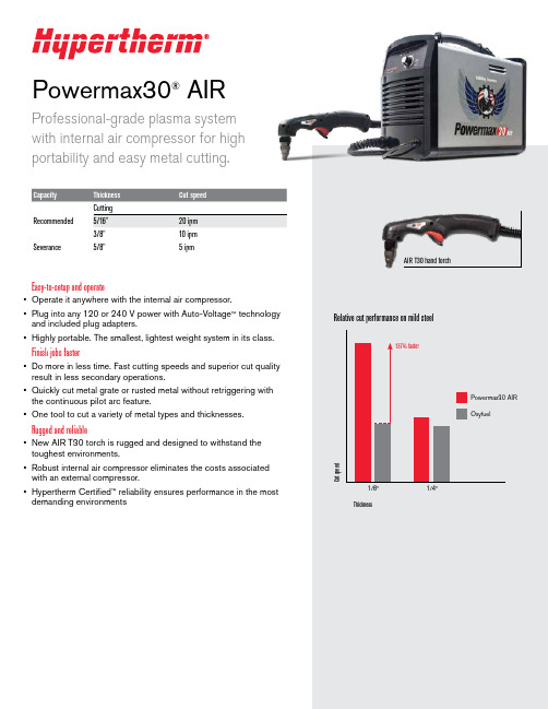
Powermax30®AIRProfessional-grade plasma system with internal air compressor for highportability and easy metal cutting.Recommended Severance5/8"5 ipmEasy-to-setup and operate• Operate it anywhere with the internal air compressor.• Plug into any 120 or 240 V power with Auto-Voltage ™ technology and included plug adapters.• Highly portable. The smallest, lightest weight system in its class.Finish jobs faster• Do more in less time. Fast cutting speeds and superior cut quality result in less secondary operations.• Quickly cut metal grate or rusted metal without retriggering with the continuous pilot arc feature.• One tool to cut a variety of metal types and thicknesses.Rugged and reliable• New AIR T30 torch is rugged and designed to withstand the toughest environments.• Robust internal air compressor eliminates the costs associated with an external compressor.• Hypertherm Certified ™ reliability ensures performance in the mostdemanding environmentsAIR T30 hand torchMoisture removal systemCompressorSystem includes• Power supply, AIR T30 hand torch with 15' lead and work clamp with 15' lead• 240 V/20 A plug with adapters for 120 V/15 A and 240 V/20 A circuits• Operator and safety manuals • 1 nozzle and 1 electrode •Carrying strapTorch consumable partsHigh performing technologyThe new patent-pending consumable designs enable consistent cutting by optimizing the air flow from the compact, internal compressor. Coupled with the highly effective moisture removal system, the Powermax30 AIR provides great cut quality and performance in hot and humid conditions.Customer testimonial“Because our company provides service in very remote places where the access for air compressors is very limited, the portability of the Powermax30 AIR with the internal compressor, makes it ideal for field services. It also eliminates the need for oxyfuel cutting, consequently reducing the cost and increasing the productivity of the cutting process.”Diego Nunes Fernando, BNG Metalmecânica, BrazilCommon applicationsHVAC, property/plant maintenance, fire and rescue, general fabrication, plus:ConstructionVehicle repair and modificationAgriculturalRecommended Hypertherm genuine accessoriesFace shieldClear face shield with flip-up shade for cutting and grinding. Safety shield included. ANSI Z87.1, CSA Z94.3, CE 127239 Face shield shade 6127103 Face shield shade 8Flip-up eyeshadesShade 5 (for <40 A) flip-up shade, anti-scratch lens and adjustable frame. ANSI Z87.1, CSA Z94.3, CE.017033 Flip-up eyeshadesHyamp ™ cutting and gouging glovesInsulated for heavy duty applications. Gun-cut palm design with seamless trigger finger and extended cuff provide flexibility and protection.017025 Medium 017026 Large 017027 X-large 017028 2X-largeSystem dust coversMade from a flame-retardant vinyl, a dust cover will protect your Powermax ® system for years. Made in USA.127469 Cover, Powermax30 AIRCircle cutting guidesQuick and easy set up for accurate circles up to 28" diameter. For optional use as a stand-off guide for straight and bevel cuts. Made in USA.127102 Basic kit – 15" arm, wheels and pivot pin027668 Deluxe kit – 11" arm, wheels, pivot pin, anchor base and plastic casePocket level and tape holderMagnetic base and tape holder with built-in level. Made in USA.017044Pocket level and tape holderEnvironmental stewardship is a core value of Hypertherm. Our Powermax products areengineered to meet and exceed global environmental regulations including the RoHS directive.Engineered and assembled in the USA ISO 9001:2008Hypertherm, Powermax, Auto-Voltage, Hypertherm Certified, and Hyamp aretrademarks of Hypertherm Inc. and may be registered in the United States and/or other countries. All other trademarks are the properties of their respective owners.©12/2014 Hypertherm Inc. Revision 0860620。
top249yn

TOP242 P or G 9 W TOP242 R 15 W TOP242 Y or F 10 W TOP243 P or G 13 W TOP243 R 29 W TOP243 Y or F 20 W TOP244 P or G 16 W TOP244 R 34 W TOP244 Y or F 30 W TOP245 P or G 19 W TOP245 R 37 W TOP245 Y or F 40 W TOP246 P or G 21 W TOP246 R 40 W TOP246 Y or F 60 W 42 W TOP247 R TOP247 Y or F 85 W 43 W TOP248 R TOP248 Y or F 105 W 44 W TOP249 R TOP249 Y or F 120 W 45 W TOP250 R TOP250 Y or F 135 W
Extended Power, Design Flexible, ® EcoSmart, Integrated Off-line Switcher
AC IN
+ DBiblioteka OUT -DLCONTROL
TOPSwitch-GX
S
C
X
F
PI-2632-060200
Figure 1. Typical Flyback Application.
Table 1. Notes: 1. Typical continuous power in a non-ventilated enclosed adapter measured at 50 °C ambient. 2. Maximum practical continuous power in an open frame design at 50 °C ambient. See Key Applications for detailed conditions. 3. For lead-free package options, see Part Ordering Information. 4. 230 VAC or 100/115 VAC with doubler.
LTE R12 协议 36212
3GPP TS 36.212 V12.0.0 (2013-12)Technical Specification3rd Generation Partnership Project;Technical Specification Group Radio Access Network;Evolved Universal Terrestrial Radio Access (E-UTRA);Multiplexing and channel coding(Release 12)The present document has been developed within the 3rd Generation Partnership Project (3GPP TM) and may be further elaborated for the purposes of 3GPP. The present document has not been subject to any approval process by the 3GPP Organizational Partners and shall not be implemented.This Specification is provided for future development work within 3GPP only. The Organizational Partners accept no liability for any use of this Specification. Specifications and reports for implementation of the 3GPP TM system should be obtained via the 3GPP Organizational Partners‟ Publications Offices.KeywordsUMTS, radio, Layer 13GPPPostal address3GPP support office address650 Route des Lucioles – Sophia AntipolisValbonne – FranceTel. : +33 4 92 94 42 00 Fax : +33 4 93 65 47 16InternetCopyright NotificationNo part may be reproduced except as authorized by written permission.The copyright and the foregoing restriction extend to reproduction in all media.© 2013, 3GPP Organizational Partners (ARIB, ATIS, CCSA, ETSI, TTA, TTC).All rights reserved.UMTS™ is a Trade Mark of ETSI registered for the benefit of its members3GPP™ is a Trade Mark of ETSI registered for the benefit of its Members and of the 3GPP Organizational Partners LTE™ is a Trade Mark of ETSI registered for the benefit of its Members and o f the 3GPP Organizational Partners GSM® and the GSM logo are registered and owned by the GSM AssociationContentsForeword (5)1Scope (6)2References (6)3Definitions, symbols and abbreviations (6)3.1 Definitions (6)3.2Symbols (6)3.3 Abbreviations (7)4Mapping to physical channels (7)4.1Uplink (7)4.2Downlink (8)5Channel coding, multiplexing and interleaving (8)5.1Generic procedures (8)5.1.1CRC calculation (8)5.1.2Code block segmentation and code block CRC attachment (9)5.1.3Channel coding (11)5.1.3.1Tail biting convolutional coding (11)5.1.3.2Turbo coding (12)5.1.3.2.1Turbo encoder (12)5.1.3.2.2Trellis termination for turbo encoder (13)5.1.3.2.3Turbo code internal interleaver (13)5.1.4Rate matching (15)5.1.4.1Rate matching for turbo coded transport channels (15)5.1.4.1.1Sub-block interleaver (15)5.1.4.1.2Bit collection, selection and transmission (16)5.1.4.2Rate matching for convolutionally coded transport channels and control information (18)5.1.4.2.1Sub-block interleaver (19)5.1.4.2.2Bit collection, selection and transmission (20)5.1.5Code block concatenation (20)5.2Uplink transport channels and control information (21)5.2.1Random access channel (21)5.2.2Uplink shared channel (21)5.2.2.1Transport block CRC attachment (22)5.2.2.2Code block segmentation and code block CRC attachment (22)5.2.2.3Channel coding of UL-SCH (23)5.2.2.4Rate matching (23)5.2.2.5Code block concatenation (23)5.2.2.6 Channel coding of control information (23)5.2.2.6.1Channel quality information formats for wideband CQI reports (33)5.2.2.6.2Channel quality information formats for higher layer configured subband CQI reports (34)5.2.2.6.3Channel quality information formats for UE selected subband CQI reports (37)5.2.2.6.4Channel coding for CQI/PMI information in PUSCH (39)5.2.2.6.5Channel coding for more than 11 bits of HARQ-ACK information (40)5.2.2.7 Data and control multiplexing (41)5.2.2.8 Channel interleaver (42)5.2.3Uplink control information on PUCCH (44)5.2.3.1Channel coding for UCI HARQ-ACK (44)5.2.3.2Channel coding for UCI scheduling request (49)5.2.3.3Channel coding for UCI channel quality information (49)5.2.3.3.1Channel quality information formats for wideband reports (49)5.2.3.3.2Channel quality information formats for UE-selected sub-band reports (52)5.2.3.4Channel coding for UCI channel quality information and HARQ-ACK (56)5.2.4Uplink control information on PUSCH without UL-SCH data (56)5.2.4.1 Channel coding of control information (57)5.2.4.2 Control information mapping (57)5.2.4.3 Channel interleaver (58)5.3Downlink transport channels and control information (58)5.3.1Broadcast channel (58)5.3.1.1Transport block CRC attachment (58)5.3.1.2Channel coding (59)5.3.1.3 Rate matching (59)5.3.2Downlink shared channel, Paging channel and Multicast channel (59)5.3.2.1Transport block CRC attachment (60)5.3.2.2Code block segmentation and code block CRC attachment (60)5.3.2.3Channel coding (61)5.3.2.4Rate matching (61)5.3.2.5Code block concatenation (61)5.3.3Downlink control information (61)5.3.3.1DCI formats (62)5.3.3.1.1Format 0 (62)5.3.3.1.2Format 1 (63)5.3.3.1.3Format 1A (64)5.3.3.1.3A Format 1B (66)5.3.3.1.4Format 1C (68)5.3.3.1.4A Format 1D (68)5.3.3.1.5Format 2 (70)5.3.3.1.5A Format 2A (73)5.3.3.1.5B Format 2B (75)5.3.3.1.5C Format 2C (76)5.3.3.1.5D Format 2D (78)5.3.3.1.6Format 3 (79)5.3.3.1.7Format 3A (79)5.3.3.1.8Format 4 (80)5.3.3.2CRC attachment (81)5.3.3.3Channel coding (82)5.3.3.4Rate matching (82)5.3.4Control format indicator (82)5.3.4.1Channel coding (83)5.3.5HARQ indicator (HI) (83)5.3.5.1Channel coding (83)Annex A (informative): Change history (85)ForewordThis Technical Specification has been produced by the 3rd Generation Partnership Project (3GPP).The contents of the present document are subject to continuing work within the TSG and may change following formal TSG approval. Should the TSG modify the contents of the present document, it will be re-released by the TSG with an identifying change of release date and an increase in version number as follows:Version x.y.zwhere:x the first digit:1 presented to TSG for information;2 presented to TSG for approval;3 or greater indicates TSG approved document under change control.Y the second digit is incremented for all changes of substance, i.e. technical enhancements, corrections, updates, etc.z the third digit is incremented when editorial only changes have been incorporated in the document.1 ScopeThe present document specifies the coding, multiplexing and mapping to physical channels for E-UTRA.2 ReferencesThe following documents contain provisions which, through reference in this text, constitute provisions of the present document.∙References are either specific (identified by date of publication, edition number, version number, etc.) or non-specific.∙For a specific reference, subsequent revisions do not apply.∙For a non-specific reference, the latest version applies. In the case of a reference to a 3GPP document (includinga GSM document), a non-specific reference implicitly refers to the latest version of that document in the sameRelease as the present document.[1] 3GPP TR 21.905: "Vocabulary for 3GPP Specifications".[2] 3GPP TS 36.211: "Evolved Universal Terrestrial Radio Access (E-UTRA); Physical channels andmodulation".[3] 3GPP TS 36.213: "Evolved Universal Terrestrial Radio Access (E-UTRA); Physical layerprocedures".[4] 3GPP TS 36.306: "Evolved Universal Terrestrial Radio Access (E-UTRA); User Equipment (UE)radio access capabilities".[5] 3GPP TS36.321, “Evolved Universal Terrestrial Radio Access (E-UTRA); Medium AccessControl (MAC) protocol specification”[6] 3GPP TS36.331, “Evolved Universal Terrestrial Radio Access (E-UTRA); Radio ResourceControl (RRC) proto col specification”3 Definitions, symbols and abbreviations3.1 DefinitionsFor the purposes of the present document, the terms and definitions given in [1] and the following apply. A term defined in the present document takes precedence over the definition of the same term, if any, in [1].Definition format<defined term>: <definition>.3.2 SymbolsFor the purposes of the present document, the following symbols apply:DLN Downlink bandwidth configuration, expressed in number of resource blocks [2] RBULN Uplink bandwidth configuration, expressed in number of resource blocks [2] RBRBN Resource block size in the frequency domain, expressed as a number of subcarriers scPUSCHN Number of SC-FDMA symbols carrying PUSCH in a subframesym b-PUSCHinitialN Number of SC-FDMA symbols carrying PUSCH in the initial PUSCH transmission subframe symbULN Number of SC-FDMA symbols in an uplink slotsymbN Number of SC-FDMA symbols used for SRS transmission in a subframe (0 or 1).SRS3.3 AbbreviationsFor the purposes of the present document, the following abbreviations apply:BCH Broadcast channelCFI Control Format IndicatorCP Cyclic PrefixCSI Channel State InformationDCI Downlink Control InformationDL-SCH Downlink Shared channelEPDCCH Enhanced Physical Downlink Control channelFDD Frequency Division DuplexingHI HARQ indicatorMCH Multicast channelPBCH Physical Broadcast channelPCFICH Physical Control Format Indicator channelPCH Paging channelPDCCH Physical Downlink Control channelPDSCH Physical Downlink Shared channelPHICH Physical HARQ indicator channelPMCH Physical Multicast channelPMI Precoding Matrix IndicatorPRACH Physical Random Access channelPUCCH Physical Uplink Control channelPUSCH Physical Uplink Shared channelRACH Random Access channelRI Rank IndicationSR Scheduling RequestSRS Sounding Reference SignalTDD Time Division DuplexingTPMI Transmitted Precoding Matrix IndicatorUCI U plink Control InformationUL-SCH Uplink Shared channel4 Mapping to physical channels4.1 UplinkTable 4.1-1 specifies the mapping of the uplink transport channels to their corresponding physical channels. Table 4.1-2 specifies the mapping of the uplink control channel information to its corresponding physical channel.Table 4.1-1Table 4.1-24.2 DownlinkTable 4.2-1 specifies the mapping of the downlink transport channels to their corresponding physical channels. Table4.2-2 specifies the mapping of the downlink control channel information to its corresponding physical channel.Table 4.2-1Table 4.2-25 Channel coding, multiplexing and interleavingData and control streams from/to MAC layer are encoded /decoded to offer transport and control services over the radio transmission link. Channel coding scheme is a combination of error detection, error correcting, rate matching, interleaving and transport channel or control information mapping onto/splitting from physical channels.5.1Generic procedures This section contains coding procedures which are used for more than one transport channel or control information type.5.1.1 CRC calculation Denote the input bits to the CRC computation by 13210,...,,,,-A a a a a a , and the parity bits by 13210,...,,,,-L p p p p p . A is the size of the input sequence and L is the number of parity bits. The parity bits are generated by one of the following cyclic generator polynomials:- g CRC24A (D ) = [D 24 + D 23 + D 18 + D 17 + D 14 + D 11 + D 10 + D 7 + D 6 + D 5 + D 4 + D 3 + D + 1] and;- g CRC24B (D ) = [D 24 + D 23 + D 6 + D 5 + D + 1] for a CRC length L = 24 and;- g CRC16(D ) = [D 16 + D 12 + D 5 + 1] for a CRC length L = 16.- g CRC8(D ) = [D 8 + D 7 + D 4 + D 3 + D + 1] for a CRC length of L = 8.The encoding is performed in a systematic form, which means that in GF(2), the polynomial:23122221230241221230......p D p D p D p D a D a D a A A A ++++++++-++yields a remainder equal to 0 when divided by the corresponding length-24 CRC generator polynomial, g CRC24A (D ) or g CRC24B (D ), the polynomial:15114141150161141150......p D p D p D p D a D a D a A A A ++++++++-++yields a remainder equal to 0 when divided by g CRC16(D ), and the polynomial:7166170816170......p D p D p D p D a D a D a A A A ++++++++-++yields a remainder equal to 0 when divided by g CRC8(D ).The bits after CRC attachment are denoted by 13210,...,,,,-B b b b b b , where B = A + L . The relation between a k and b k is:k k a b = for k = 0, 1, 2, …, A -1A k k p b -=for k = A , A +1, A +2,..., A +L -1.5.1.2 Code block segmentation and code block CRC attachmentThe input bit sequence to the code block segmentation is denoted by 13210,...,,,,-B b b b b b , where B > 0. If B is larger than the maximum code block size Z , segmentation of the input bit sequence is performed and an additional CRC sequence of L = 24 bits is attached to each code block. The maximum code block size is:- Z = 6144.If the number of filler bits F calculated below is not 0, filler bits are added to the beginning of the first block.Note that if B < 40, filler bits are added to the beginning of the code block.The filler bits shall be set to <NULL > at the input to the encoder.Total number of code blocks C is determined by:if Z B ≤L = 0Number of code blocks: 1=C B B ='elseL = 24Number of code blocks: ()⎡⎤L Z B C -=/. L C B B ⋅+='end ifThe bits output from code block segmentation, for C ≠ 0, are denoted by ()13210,...,,,,-r K r r r r r c c c c c , where r is the code block number, and K r is the number of bits for the code block number r .Number of bits in each code block (applicable for C ≠ 0 only):First segmentation size: +K = minimum K in table 5.1.3-3 such that B K C '≥⋅if 1=Cthe number of code blocks with length +K is +C =1, 0=-K , 0=-Celse if 1>CSecond segmentation size: -K = maximum K in table 5.1.3-3 such that +<K K -+-=∆K K KNumber of segments of size -K : ⎥⎦⎥⎢⎣⎢∆'-⋅=+-K B K C C . Number of segments of size +K : -+-=C C C .end ifNumber of filler bits: B K C K C F '-⋅+⋅=--++for k = 0 to F -1-- Insertion of filler bits >=<NULL c k 0end fork = Fs = 0for r = 0 to C -1if -<C r-=K K relse+=K K rend ifwhile L K k r -<s rk b c =1+=k k1+=s s end whileif C >1The sequence ()13210,...,,,,--L K r r r r r r c c c c c is used to calculate the CRC parity bits ()1210,...,,,-L r r r r p p p paccording to section 5.1.1 with the generator polynomial g CRC24B (D ). For CRC calculation it isassumed that filler bits, if present, have the value 0.while r K k <)(r K L k r rk p c -+=1+=k kend whileend if 0=kend for5.1.3 Channel codingThe bit sequence input for a given code block to channel coding is denoted by 13210,...,,,,-K c c c c c , where K is thenumber of bits to encode. After encoding the bits are denoted by )(1)(3)(2)(1)(0,...,,,,i D i i i i d d d d d -, where D is the number of encoded bits per output stream and i indexes the encoder output stream. The relation between k c and )(i k d and betweenK and D is dependent on the channel coding scheme.The following channel coding schemes can be applied to TrCHs: - tail biting convolutional coding; - turbo coding.Usage of coding scheme and coding rate for the different types of TrCH is shown in table 5.1.3-1. Usage of coding scheme and coding rate for the different control information types is shown in table 5.1.3-2. The values of D in connection with each coding scheme: - tail biting convolutional coding with rate 1/3: D = K ; - turbo coding with rate 1/3: D = K + 4.The range for the output stream index i is 0, 1 and 2 for both coding schemes.Table 5.1.3-1: Usage of channel coding scheme and coding rate for TrCHs.Table 5.1.3-2: Usage of channel coding scheme and coding rate for control information.5.1.3.1 Tail biting convolutional codingA tail biting convolutional code with constraint length 7 and coding rate 1/3 is defined. The configuration of the convolutional encoder is presented in figure 5.1.3-1.The initial value of the shift register of the encoder shall be set to the values corresponding to the last 6 information bits in the input stream so that the initial and final states of the shift register are the same. Therefore, denoting the shift register of the encoder by 5210,...,,,s s s s , then the initial value of the shift register shall be set to()i K i c s --=10 = 133 (octal)1 = 171 (octal)2 = 165 (octal)Figure 5.1.3-1: Rate 1/3 tail biting convolutional encoder.The encoder output streams )0(k d , )1(k d and )2(k d correspond to the first, second and third parity streams, respectively asshown in Figure 5.1.3-1.5.1.3.2Turbo coding5.1.3.2.1Turbo encoderThe scheme of turbo encoder is a Parallel Concatenated Convolutional Code (PCCC) with two 8-state constituent encoders and one turbo code internal interleaver. The coding rate of turbo encoder is 1/3. The structure of turbo encoder is illustrated in figure 5.1.3-2.The transfer function of the 8-state constituent code for the PCCC is: G (D ) = ⎥⎦⎤⎢⎣⎡)()(,101D g D g ,whereg 0(D ) = 1 + D 2 + D 3,g 1(D ) = 1 + D + D 3.The initial value of the shift registers of the 8-state constituent encoders shall be all zeros when starting to encode the input bits.The output from the turbo encoder isk k x d =)0( k k z d =)1( k k z d '=)2(for 1,...,2,1,0-=K k .If the code block to be encoded is the 0-th code block and the number of filler bits is greater than zero, i.e., F > 0, thenthe encoder shall set c k , = 0, k = 0,…,(F -1) at its input and shall set >=<NULL d k )0(, k = 0,…,(F -1) and >=<NULL d k )1(, k = 0,…,(F -1) at its output.The bits input to the turbo encoder are denoted by 13210,...,,,,-K c c c c c , and the bits output from the first and second 8-state constituent encoders are denoted by 13210,...,,,,-K z z z z z and 13210,...,,,,-'''''K z z z z z , respectively. The bits outputfrom the turbo code internal interleaver are denoted by 110,...,,-'''K c c c , and these bits are to be the input to the second 8-state constituent encoder.Figure 5.1.3-2: Structure of rate 1/3 turbo encoder (dotted lines apply for trellis termination only).5.1.3.2.2 Trellis termination for turbo encoderTrellis termination is performed by taking the tail bits from the shift register feedback after all information bits areencoded. Tail bits are padded after the encoding of information bits.The first three tail bits shall be used to terminate the first constituent encoder (upper switch of figure 5.1.3-2 in lower position) while the second constituent encoder is disabled. The last three tail bits shall be used to terminate the second constituent encoder (lower switch of figure 5.1.3-2 in lower position) while the first constituent encoder is disabled. The transmitted bits for trellis termination shall then be:K K x d =)0(, 1)0(1++=K K z d , K K x d '=+)0(2, 1)0(3++'=K K z d K K z d =)1(, 2)1(1++=K K x d , K K z d '=+)1(2, 2)1(3++'=K K x d1)2(+=K K x d , 2)2(1++=K K z d , 1)2(2++'=K K x d , 2)2(3++'=K K z d5.1.3.2.3 Turbo code internal interleaverThe bits input to the turbo code internal interleaver are denoted by 110,...,,-K c c c , where K is the number of input bits.The bits output from the turbo code internal interleaver are denoted by 110,...,,-'''K c c c . The relationship between the input and output bits is as follows:()i i c c ∏=', i =0, 1,…, (K -1)where the relationship between the output index i and the input index )(i ∏ satisfies the following quadratic form:()K i f i f i mod )(221⋅+⋅=∏The parameters 1f and 2f depend on the block size K and are summarized in Table 5.1.3-3.Table 5.1.3-3: Turbo code internal interleaver parameters.5.1.4Rate matching5.1.4.1Rate matching for turbo coded transport channelsThe rate matching for turbo coded transport channels is defined per coded block and consists of interleaving the threeinformation bit streams )0(k d , )1(k d and )2(k d , followed by the collection of bits and the generation of a circular buffer asdepicted in Figure 5.1.4-1. The output bits for each code block are transmitted as described in section 5.1.4.1.2.Figure 5.1.4-1. Rate matching for turbo coded transport channels.The bit stream )0(k d is interleaved according to the sub-block interleaver defined in section 5.1.4.1.1 with an output sequence defined as )0(1)0(2)0(1)0(0,...,,,-∏K v v v v and where ∏K is defined in section 5.1.4.1.1.The bit stream )1(k d is interleaved according to the sub-block interleaver defined in section 5.1.4.1.1 with an output sequence defined as )1(1)1(2)1(1)1(0,...,,,-∏K v v v v .The bit stream )2(k d is interleaved according to the sub-block interleaver defined in section 5.1.4.1.1 with an output sequence defined as )2(1)2(2)2(1)2(0,...,,,-∏K v v v v .The sequence of bits k e for transmission is generated according to section 5.1.4.1.2.5.1.4.1.1 Sub-block interleaverThe bits input to the block interleaver are denoted by )(1)(2)(1)(0,...,,,i D i i i d d d d -, where D is the number of bits. The output bit sequence from the block interleaver is derived as follows:(1) Assign 32=TCsubblockC to be the number of columns of the matrix. The columns of the matrix are numbered 0, 1, 2,…,1-TCsubblockC from left to right. (2) Determine the number of rows of the matrix TCsubblock R , by finding minimum integer TCsubblock R such that:()TCsubblock TC subblock C R D ⨯≤The rows of rectangular matrix are numbered 0, 1, 2,…,1-TCsubblockR from top to bottom.(3) If ()D C R TC subblock TC subblock >⨯, then ()D C R N TCsubblock TC subblock D -⨯= dummy bits are padded such that y k = <NULL > for k = 0, 1,…, N D - 1. Then, )(i k k N d y D =+, k = 0, 1,…, D -1, and the bit sequence y k is written intothe ()TC subblockTC subblock C R ⨯ matrix row by row starting with bit y 0 in column 0 of row 0: ⎥⎥⎥⎥⎥⎦⎤⎢⎢⎢⎢⎢⎣⎡-⨯+⨯-+⨯-⨯--++-)1(2)1(1)1()1(12211210TCsubblock TC subblock TCsubblock TCsubblock TCsubblock TCsubblock TCsubblockTC subblock TCsubblock TCsubblock TCsubblock TCsubblock TCsubblock C R C R C R C R C C C C C y y y y y y y y y y y yFor )0(k d and )1(k d :(4) Perform the inter-column permutation for the matrix based on the pattern (){}1,...,1,0-∈TCsubblock C j j P that is shown intable 5.1.4-1, where P(j ) is the original column position of the j -th permuted column. After permutation of thecolumns, the inter-column permuted ()TCsubblockTC subblock C R ⨯ matrix is equal to ⎥⎥⎥⎥⎥⎦⎤⎢⎢⎢⎢⎢⎣⎡⨯-+-⨯-+⨯-+⨯-++-+++-TCsubblockTC subblock TCsubblock TCsubblockTCsubblock TCsubblockTCsubblock TCsubblock TC subblock TCsubblockTCsubblock TCsubblockTCsubblockTCsubblock TC subblock C R C P C R P C R P C R P C C P C P C P C P C P P P P y y y y y y y y y y y y )1()1()1()2()1()1()1()0()1()2()1()0()1()2()1()0((5) The output of the block interleaver is the bit sequence read out column by column from the inter-columnpermuted ()TCsubblockTC subblock C R ⨯matrix. The bits after sub-block interleaving are denoted by )(1)(2)(1)(0,...,,,i K i i i v v v v -∏,where )(0i v corresponds to )0(P y ,)(1i v to TC subblockC P y +)0(… and ()TCsubblock TC subblock C R K ⨯=∏.For )2(k d :(4) The output of the sub-block interleaver is denoted by )2(1)2(2)2(1)2(0,...,,,-∏K v v v v , where )()2(k ky v π= and where ()∏⎪⎪⎭⎫ ⎝⎛+⨯+⎪⎪⎭⎫ ⎝⎛⎥⎥⎦⎥⎢⎢⎣⎢=K R k C R k P k TC subblock TC subblock TC subblock mod 1mod )(π The permutation function P is defined in Table 5.1.4-1.Table 5.1.4-1 Inter-column permutation pattern for sub-block interleaver.5.1.4.1.2 Bit collection, selection and transmissionThe circular buffer of length ∏=K K w 3 for the r -th coded block is generated as follows: )0(k k v w =for k = 0,…, 1-∏K)1(2k k K v w =+∏ for k = 0,…, 1-∏K)2(12k k K v w =++∏ for k = 0,…, 1-∏KDenote the soft buffer size for the transport block by N IR bits and the soft buffer size for the r -th code block by N cb bits. The size N cb is obtained as follows, where C is the number of code blocks computed in section 5.1.2: -⎪⎪⎭⎫⎝⎛⎥⎦⎥⎢⎣⎢=w IR cb K C N N ,min for DL-SCH and PCH transport channels- w cb K N = for UL-SCH and MCH transport channelswhere N IR is equal to:()⎥⎥⎦⎥⎢⎢⎣⎢⋅⋅=limit DL_HARQ MIMO ,min M M K K N N C soft IRwhere:If the UE signals ue-Category-v1020, and is configured with transmission mode 9 or transmission mode 10 for the DLcell, N soft is the total number of soft channel bits [4] according to the UE category indicated by ue-Category-v1020 [6]. Otherwise, N soft is the total number of soft channel bits [4] according to the UE category indicated by ue-Category (without suffix) [6]. If N soft = 35982720, K C = 5,elseif N soft = 3654144 and the UE is capable of supporting no more than a maximum of two spatial layers for the DL cell, K C = 2 else K C = 1 End if.K MIMO is equal to 2 if the UE is configured to receive PDSCH transmissions based on transmission modes 3, 4, 8, 9 or 10 as defined in section 7.1 of [3], and is equal to 1 otherwise.If the UE is configured with more than one serving cell and if at least two serving cells have different UL/DLconfigurations, M DL_HARQ is the maximum number of DL HARQ processes as defined in Table 7-1 in [3] for the DL-reference UL/DL configuration of the serving cell. Otherwise, M DL_HARQ is the maximum number of DL HARQ processes as defined in section 7 of [3]. M limit is a constant equal to 8.Denoting by E the rate matching output sequence length for the r -th coded block, and rv idx the redundancy version number for this transmission (rv idx = 0, 1, 2 or 3), the rate matching output bit sequence is k e , k = 0,1,..., 1-E . Define by G the total number of bits available for the transmission of one transport block.Set )m L Q N G G ⋅=' where Q m is equal to 2 for QPSK, 4 for 16QAM and 6 for 64QAM, and where - For transmit diversity: - N L is equal to 2, - Otherwise:- N L is equal to the number of layers a transport block is mapped onto Set C G mod '=γ, where C is the number of code blocks computed in section 5.1.2.if 1--≤γC rset ⎣⎦C G Q N E m L /'⋅⋅= elseset ⎡⎤C G Q N E m L /'⋅⋅=end if Set ⎪⎪⎭⎫ ⎝⎛+⋅⎥⎥⎤⎢⎢⎡⋅⋅=2820idx TC subblock cb TCsubblockrv R N R k , where TC subblock R is the number of rows defined in section 5.1.4.1.1. Set k = 0 and j = 0 while { k < E } if >≠<+NULL w cb N j k m od )(0 cb N j k k w e m od )(0+=k = k +1end if j = j +1end while5.1.4.2Rate matching for convolutionally coded transport channels and control informationThe rate matching for convolutionally coded transport channels and control information consists of interleaving thethree bit streams, )0(k d , )1(k d and )2(k d , followed by the collection of bits and the generation of a circular buffer asdepicted in Figure 5.1.4-2. The output bits are transmitted as described in section 5.1.4.2.2.Figure 5.1.4-2. Rate matching for convolutionally coded transport channels and control information.The bit stream )0(k d is interleaved according to the sub-block interleaver defined in section 5.1.4.2.1 with an output sequence defined as )0(1)0(2)0(1)0(0,...,,,-∏K v v v v and where ∏K is defined in section 5.1.4.2.1.The bit stream )1(k d is interleaved according to the sub-block interleaver defined in section 5.1.4.2.1 with an output sequence defined as )1(1)1(2)1(1)1(0,...,,,-∏K v v v v .。
Calculation of AGARD Wing 445.6 Flutter Using Navier-Stokes Aerodynamics

NASA Langley Research Center Hampton, Virginia 23681–0001
Abstract
The flutter characteristics of the first AGARD standard aeroelastic configuration for dynamic response, Wing 445.6, are studied using an unsteady Navier-Stokes algorithm in order to investigate a previously noted discrepancy between Euler flutter characteristics and the experimental data. The algorithm, which is a three-dimensional, implicit, upwind Euler/Navier-Stokes code (CFL3D Version 2.1), was previously modified for the time-marching, aeroelastic analysis of wings using the unsteady Euler equations. These modifications include the incorporation of a deforming mesh algorithm and the addition of the structural equations of motion for their simultaneous time integration with the governing flow equations. In this paper, the aeroelastic method is extended and evaluated for applications that use the NavierStokes aerodynamics. The paper presents a brief description of the aeroelastic method and presents unsteady calculations which verify this method for Navier-Stokes calculations. A linear stability analysis and a time-marching aeroelastic analysis are used to determine the flutter characteristics of the isolated 45 swept-back wing. Effects of fluid viscosity, structural damping, and number of modes in the structural model are investigated. For the linear stability analysis, the unsteady generalized aerodynamic forces of the wing are computed for a range of reduced frequencies using the pulse transfer-function approach. The flutter characteristics of the wing are determined using these unsteady generalized aerodynamic forces in a traditional V-g analysis. This stability analysis is used to determine the flutter characteristics of the wing at free-stream Mach numbers of 0.96 and 1.141 using the generalized aerodynamic forces generated by solving the Euler equations and the Navier-Stokes equations. Time-marching aeroelastic calculations are performed at a free-stream Mach number of 1.141vier-Stokes equations to compare with the linear V-g flutter analysis method. The V-g analysis, which is used in conjunction with the time-marching analysis, indicates that the fluid viscosity has a significant effect on the
- 1、下载文档前请自行甄别文档内容的完整性,平台不提供额外的编辑、内容补充、找答案等附加服务。
- 2、"仅部分预览"的文档,不可在线预览部分如存在完整性等问题,可反馈申请退款(可完整预览的文档不适用该条件!)。
- 3、如文档侵犯您的权益,请联系客服反馈,我们会尽快为您处理(人工客服工作时间:9:00-18:30)。
Performance-Guarantee Gene Predictions via Spliced AlignmentAndrey A.Mironov,*,1Michael A.Roytberg,†Pavel A.Pevzner,‡,2and Mikhail S.Gelfand §*Laboratory of Mathematical Methods,National Center for Biotechnology NIIGENETIKA,Moscow 113545,Russia;†Institute of Mathematical Problems of Biology and §Institute of Protein Research,Russian Academy of Sciences,Puschino,Moscow region 142292,Russia;and ‡Departments of Mathematics and Computer Science,University of Southern California,Los Angeles,California 90089-1113Received March 5,1997;accepted January 29,1998An important and still unsolved problem in gene prediction is designing an algorithm that not only pre-dicts genes but estimates the quality of individual pre-dictions as well.Since experimental biologists are interested mainly in the reliability of individual pre-dictions (rather than in the average reliability of an algorithm)we attempted to develop a gene recogni-tion algorithm that guarantees a certain quality of predictions.We demonstrate here that the similarity level with a related protein is a reliable quality esti-mator for the spliced alignment approach to gene rec-ognition.We also study the average performance of the spliced alignment algorithm for different targets on a complete set of human genomic sequences with known relatives and demonstrate that the average performance of the method remains high even for very distant ing plant,fungal,and prokaryotic target proteins for recognition of human genes leads to accurate predictions with 95,93,and 91%correla-tion coefficient,respectively.For target proteins with similarity score above 60%,not only the average cor-relation coefficient is very high (97%and up)but also the quality of individual predictions is guaranteed to be at least 82%.It indicates that for this level of simi-larity the worst case performance of the spliced align-ment algorithm is better than the average case perfor-mance of many statistical gene recognition methods.©1998Academic PressINTRODUCTIONThe large-scale sequencing projects have motivated the need in a new generation of algorithms for compu-tational gene recognition in long uncharacterized DNA sequences.Recently the traditional statistical ap-proach to recognition of protein-coding genes was sup-plemented by similarity-based approaches (for techni-cal reviews on computer-assisted functional mapping of DNA sequences see Gelfand,1995;Fickett,1996a;introduction for users is in Fickett,1996b).Similarity search can be used to detect genes (Gish and States,1993)and,in conjunction with the statistical analysis,to predict exon–intron structure of eukaryote genes.Indeed,similarity to an already known gene can pro-vide additional statistical parameters (Snyder and Stormo,1995),allow the program to choose between several suboptimal genes (Rogozin et al.,1996),and serve as the main scoring function for candidate pro-tein-coding segments (Hultner et al.,1994).Some ex-isting servers perform database simiarity search for a predicted gene as a standard postprocessing procedure (Uberbacher et al.,1996).These approaches utilize the large amount of previously sequenced DNA and are likely to become the method of choice in the future.Consistent realization of the similarity-based gene recognition is provided by the spliced alignment algo-rithm implemented in Procrustes software (Gelfand et al.,1996a).The algorithm explores all possible exon assemblies in polynomial time and finds the multiexon structure with the best fit to a related protein.This is the main feature of the algorithm distinguishing it from other programs.Given a genomic sequence,the spliced alignment al-gorithm first finds candidate exons.This can be done by selecting all sequence fragments between potential ac-ceptor and donor sites (i.e.,between AG and GU dinucleotides)with further filtration of this set (in a way that does not lose the actual exons).The resulting set,of course,can contain many false exons,and cur-rently it is impossible to distinguish all actual exons from this set by statistical methods.Instead,the spliced alignment algorithm explores all possible as-semblies of potential exons and finds an assembly with the highest similarity to the related target protein.One of the main problems in gene recognition is designing an algorithm that would not only predict genes,but estimate the quality of individual predic-tions as well.The average performance of an algorithm can be estimated using correlation between the pre-dicted and the correct gene structure (Burset and Guigo,1996).However,in a real situation the correct1Current address:AnchorGen,Santa Monica,CA 90403.2To whom correspondence should be addressed.Telephone:(213)740-2407.E-mail:ppevzner@.GENOMICS51,332–339(1998)ARTICLE NO .GE9852513320888-7543/98$25.00Copyright ©1998by Academic PressAll rights of reproduction in any form reserved.gene structure is unknown,and no algorithm provides an estimate for the quality of obtained gene predic-tions.At best,some algorithms assign quality indica-tors to particular exons (Uberbacher and Mural,1991).Since experimental biologists are more interested in reliability of individual predictions than in the average performance,it is important to develop gene recogni-tion algorithms with guaranteed prediction quality.Recently Sze and Pevzner (1997)used the quality and certainty of fit of a candidate exon to the respective region in the target protein as an indicator of the prediction quality of individual exons.For human genes predicted by spliced alignment with mammalian targets all exons are guaranteed to be correct in one-third of cases,and at least one exon is guaranteed in half of cases.The present study analyzes the overall certainty of spliced alignment predictions with both mammalian and more distant targets and provides the estimate and bounds for the correlation coefficient between the predicted and the actual gene given the obtained sim-ilarity score.The spliced alignment algorithm is tested on the set of all completely sequenced human genes with a known related protein from another species.We study the dependence between the level of protein sim-ilarity and the accuracy of predictions and determine the ranges of guaranteed performance.In particular,we demonstrate that if the similarity score is 60Ϯ5%,the average correlation is 95%,whereas the correlation for individual predictions is always higher than 75%;it is higher than 80%in more than 97%of cases and higher than 95%in more than 70%of cases,and the prediction is exact in approximately half of all cases.We assume that predictions with a similarity score exceeding 30%are reliable and consider the remaining predictions tentative.At that,the average correlation of reliable predictions for all groups of eukaryotic tar-gets,including plants and fungi,exceeds 93%,and it is 91%for prokaryotic targets.The accuracy of tentative predictions is lower but still higher than the accuracy of statistical gene recognition algorithms as long as the similarity score is above 20%.We also analyze various filtration procedures and demonstrate that strongerfiltration provides better results for distant targets despite the danger of overfiltering true exons.DATAAll human DNA sequences from GenBank (Benson et al.,1997)and EMBL (Stoesser et al.,1997)containing completely sequenced genes were considered.This was done by automated search for text terms complete gene or complete CDS in the human divisions of GenBank and EMBL (Spring 1996releases).This preliminary list was supplemented by sequences from Snyder and Stormo (1995),Burset and Guigo (1996),and Gelfand et al.(1996b).A syntactic check was performed first on feature tables to exclude mRNA genes,incomplete and alter-natively spliced genes,sequence fragments containing multiple genes,and entries with errors in feature ta-bles (in-frame stop codons,missing start or stop codons).We also removed genes with introns shorter than 70nucleotides,which do not occur in human genes (Sharp,1994)and are an indication of an error in the feature table.Genes having unconventional splic-ing sites breaking the GU–AG rule also were removed.Such sites occur in less than 1%of human genes (Jack-son,1991).Target sequences were selected using the Entrez browser (Schuler et al.,1996).Fifteen genes having no nonprimate relatives and all histone genes were ex-cluded from the sample.For each gene one highest scoring target protein in each of the following catego-ries was considered:mammals (not primates),birds,cold-blooded vertebrates,insects,other animals,plants,fungi,other eukaryotes,and prokaryotes.Genes having the same highest scoring mammalian relatives were considered homologous.Only the long-est genomic sequence fragment from each group of homologues was retained.Distribution of local similar-ities (negative logarithms of BLAST probabilities as given in Entrez )is shown in Table 1.The resulting sample consists of 256sequences and is available from the Procrustes WWW site.The aver-age sequence length is approximately 8100nucleo-TABLE 2Distribution of the Length of Genomic DNALength (kb)Ͻ55–1010–1515–2020–3030–4055180No.of seq.126812585911TABLE 1Distribution of the Local Similarities (Negative Logarithms of BLAST Scores)Entrez score Ͻ3345678910–1112–1314–15No.of seq.05302223181411292627Entrez score 16–1718–1920–2930–3940–4950–5960–99100ϩNo.of seq.1719917454379585333GENE PREDICTIONS VIA SPLICED ALIGNMENTtides;the longest sequence in the sample exceeds 180,000nucleotides.The distribution of sequence lengths is shown in Table2.The number of exons in genes ranges from1to54(Table3),and their mini-mum length is3bp for initial exons,17bp for internal exons,and5bp for terminal exons(Table4).METHODSFiltration.Initially all initial exons bounded by a start codon ϽATG and a candidate donor siteϾGT,internal exons bounded by an acceptor site AGϽand a donor siteϾGT,terminal exons bounded by an acceptor site AGϽand a stop codonϾTGA,ϾTAA,orϾTAG are considered(ϽandϾdenote the left and right boundaries of a coding region,respectively).Note that we use the term exon as a synonym for translated part of an exon,which is the traditional although biologically incorrect use of this term in computational molecular biology.Internal exons should be longer than16nucleotides. Filtration consists of two weakfilters removing clearly abnormal exons and afinalfilter of adjustable strictness.Thefirstfilter removes exons with weak splicing sites as estimated by positional nucleotide weight matrices(Gelfand et al.,1996b).The threshold is set very low and only two actual acceptor sites are filtered out at this step.At the second step the genomic sequence is divided into subfrag-ments of length10kb with2.5kb of overlap.Furtherfiltration is performed independently in each subfragment and the candidate exons are evaluated by a scoring function taking into account strength of the splicing sites and the coding potential(Gelfand et al., 1996b).One thousand highest scoring exons are retained in each subfragment.Thisfilter loses10actual exons:1initial,6internal, and3terminal.Overall,the two preliminaryfilters decrease the number of candi-date exons approximately15-fold,while losing12actual exons in the entire sample.It should be noted that the statistical properties of these exons are so unusual that they will likely be lost by any conventional gene recognition algorithm.At the same time,prelim-inaryfiltering sharply decreases the number of candidate exons, making thefinalfilter more robust.At the mainfiltration step chains of exons of length1through3 with consistent reading frame(no in-frame stop codons)and introns longer than70nucleotides are considered.Each chain is scored by the statistics-based function.Denote the score of a chain⌫byԽ⌫Խ.An exon score is now defined as eitherP͑e͒ϭ⌫ʯe e c|⌫|,where c is somefixed constant(partition function rescoring),orB͑e͒ϭmax⌫ʯe|⌫|(best chain rescoring).The candidate exons are then ranked in the decreasing order of their scores and the given proportion of exons is retained for the spliced alignment procedure.The ranking is performed indepen-dently for initial,internal,and terminal exons.The proportion of these three classes of exons in thefilter output is1:3:1,respec-tively.Thus thefiltering is controlled by two switches(the maximal number of exons in chains Eϭ1,2,or3and the use of P or B scores) and thefiltration stringency parameter F.This parameter deter-mines the number of exons dependent on the genomic sequence length.Following preliminary analysis,three values of this param-eter have been considered:1exon per14nucleotides(Fϭ14,weak filtration),1exon per33nucleotides(Fϭ33,moderatefiltration), and1exon per100nucleotides(Fϭ100strongfiltration).Note that if Eϭ1allfilters coincide.Table5presents the results of comparison of differentfilters. Filters based on chains of two and three exons(Eϭ2or Eϭ3) outperform single-exonfilters(Eϭ1)in the entire range offiltration stringency.The best weakfiltration mode(Fϭ14)seems to be partition function rescoring(P)with two-exon chains(Eϭ2).Relaxing the filtration parameters further does not recover more than one lost exon,while adding many more false exons.The optimal mode for moderate and strongfiltration(Fϭ33and Fϭ100)is best structure rescoring(B)with three-exon chains(Eϭ3).These options werefixed for further analysis.Single-exon genes were considered separately in an analogous manner.The minimum length of such genes was set to180nucleo-tides;one candidate exon was retained per200bp of the genomic sequence.Spliced alignment.UNIX version of the Procrustes was used for the sample processing.The WWW version is available at /software/procrustes.The spliced alignment score was computed using PAM120 amino acid substitution matrix(Altschul,1991)with linear gapTABLE3Distribution of the Number of Exons in Human GenesNo.of exons123–56–1011–2021–303854 No.of seq.28261117016311TABLE4Distribution of the Exon Lengths in202Human Genes with Three or More Exons202initial exons:average length155bp,min.length3bp,max.length3051bpLen.1–56–1011–2021–3031–5051–7576–100101–150151–200201–300301–1000Ͼ1000 No.33116204725361516173 907internal exons:average length139bp,min.length17bp,max.length885bpLen.1–2021–2526–3031–4041–5051–7576–100100–125126–150151–200200–300Ͼ300 No.16421249311116415919510326202terminal exons:average length191bp,min.length5bp,max.length1546bpLen.1–56–1011–2021–3031–5051–7576–100101–150151–200201–300301–1000Ͼ1000 No.1267112119543516273 334MIRONOV ET AL.penalties (the preliminary analysis demonstrated that the influ-ence of the matrix on the algorithm performance is minor;other gap scoring schemes were implemented).This score was normal-ized by division of the score of the (trivial)alignment of the target protein with itself.The quality of prediction was assessed using the correlation coefficient between the predicted and the actual genes,C ϭT P ⅐T N ϪF P ⅐F Nͱ͑T P ϩF P ͒⅐͑T N ϩF N ͒⅐͑T P ϩF N ͒⅐͑T N ϩF P ͒,where T P and T N are the numbers of correctly predicted coding (true positive)and noncoding (true negative)nucleotides,respectively,F N is the number of missed coding (false negative)nucleotides,and F P is the number of noncoding nucleotides predicted to be coding (false positive).RESULTSThe average correlation coefficients for different groups of targets are presented at Table 6.It should be noted,however,that the target group is a very rough indicator of the expected prediction quality,since the mutation rates differ significantly between protein families within the same species.Further,since the targets have been chosen by the BLAST database search (via Entrez ),many targets have only local sim-ilarities with the analyzed genes and thus produce artifacts when the (global)spliced alignment is per-formed.A better indication of the expected recognition quality is provided by the normalized spliced align-ment score.The scatter plots of the correlation coef-ficient versus the alignment score (Fig.1)demon-strate that high prediction quality is guaranteed if the alignment score is high.The same figures feature plots of similarity levels providing 100,95,90,and 80%guarantee of obtaining the desired correlation coefficient given the observed alignment score and the plot of the average correlation coefficient for the given alignment score.The plots in Fig.2provide an estimate for the proportion of predictions having the correlation exceeding 80–100%given the alignment score.Superimposed filtration plots (Fig.3)demonstrate tein,the weak filter provides better recognition.However,as the distance between the analyzed gene and the target increases,moderate filtration be-comes beneficial.An explanation for this phenome-non is that stronger filtration decreases the number of candidate exons and thus eliminates competitors for the true exons when the similarity is low.How-ever,the strong filtration (one candidate exon per 100nucleotides)loses too many true exons,and its performance is inferior compared both to the weak and to the moderate filtration at the entire range of distances (data are not shown).The same results can be seen on Table 7,in which results of predictions with the alignment score higher than 30%are given.These data confirm the above observation:weak filtration provides better results with mammalian targets,whereas moderate filtration is preferable with more distant target groups.DISCUSSIONAn important feature of the spliced alignment algo-rithm is the possibility of estimating the reliability of anTABLE 5Comparison of Different FiltrationsE F100503325201410No filter 1—1171601862022142242392562P 1481922102192282392402562B 1441731982142292342402563P 1381802062212302362412563B162198218227231234240256Note.In each cell the number of sequences in which no overfiltration occurs is nes:type of filtration described by E —number of exons in chains;P or B —resp.partition function rescoring or best structure rescoring.Columns:F —stringency of filtration (sequence length divided by the number of candidate exons).TABLE 6Results of Prediction for Different Groups of TargetsTargetN W M S Human 25699.598.494.9Mammals 25296.996.493.2Birds9488.289.788.0Cold-blooded vertebrates 9887.988.387.2Invertebrates 6076.876.771.6Other animals 3978.078.373.1Plants 3786.286.982.6Fungi4584.985.478.6Other eukaryotes 1484.185.575.2Prokaryotes3279.981.778.3Note.The average correlation coefficients are shown.Columns:N —number of genes with targets from the given group;W—weak filtration (F ϭ14,E ϭ2,partition function rescoring);M—moderate filtration (F ϭ33,E ϭ3,best structure rescoring);S—strong filtra-tion (F ϭ100,E ϭ3,best structure rescoring).The first lane (“hu-man”)corresponds to the spliced alignment with the encoded protein itself as the target and is presented to demonstrate the influence of 335GENE PREDICTIONS VIA SPLICED ALIGNMENTindividual prediction by the spliced alignment score.Plot of the alignment score along the sequence(provided by Procrustes WWW server)allows one to view the rela-tively more or less reliable regions of the prediction.A different approach to the estimation of prediction reliabil-ity,based on construction of suboptimal spliced align-ments and assigning the quality offit to individual exons,Most errors of the spliced alignment occur when there are unrelated domains in the target and the analyzed gene.This situation can be diagnosed by a very low spliced alignment score,and indeed,compar-ison of Tables6and7demonstrates that setting a recognition threshold sharply improves the average correlation between predicted and actual genes.InFIG.1.Dependence of the correlation coefficient on the spliced alignment score.Scatter plot:spliced alignment score(horizontal axis), correlation coefficient(vertical axis);numerous points in the right upper corner are suppressed.Upper curve:average correlation coefficient. Other curves:correlation coefficient guaranteed with certainty pϭ100,95,90,80(upward).If a curve p passes a point(s,c),then at least p among predictions with the score s have the correlation coefficient exceeding c.Top plot:weakfiltering.Bottom plot:moderatefiltering. 336MIRONOV ET AL.alignment of the conserved regions only.This is an objective for further development.Based on computer simulations,Gelfand et al.(1996a)suggested that spliced alignment with rela-targets,despite the risk of losing some true exons due to overfiltration.This conjecture was based on the fol-lowing reasoning:the loss of some true exons is justi-fied by the strong reduction of the number of candidateFIG.2.Certainty level for predictions given the spliced alignment score.Horizontal axis—alignment score.Vertical axis—proportion of sequences with the correlation coefficient exceeding the given threshold.Plots correspond to thresholds c ϭ80,90,95,100%(from top down).If a curve c passes a point (s,p ),then at least p among predictions with the score s have the correlation coefficient exceeding c .Top plot:weak filtering.Bottom plot:moderate filtering.337GENE PREDICTIONS VIA SPLICED ALIGNMENTnumber of variants for the spliced alignment algorithm and sharp improvement of the alignment-based predic-tions for diverged targets.This conjecture has been confirmed by the present analysis which used not only close,but some very dis-tant targets(Table1).However,excessively strongfil-tration(one candidate exon per100nucleotides)loses too many true exons.The tradeoff between overfiltra-tion and excessive combinatorialflexibility depends on the similarity level,and the shift from weak to moder-atefiltration occurs at approximately50%similarity level,as measured by the spliced alignment score(Fig.3).It should be noted,however,that even for very close targets somefiltration is necessary due to the mosaic effect(Sze and Pevzner,1997).Further development of Procrustes is directed toward construction of the local spliced alignment for analysis of genomic fragments containing incomplete genes(this is simple algorithmically,but additional work is required to derive scoring schemes and reliability indicators)and spliced alignment with nucleic acid targets applicable for gene recognition given noisy EST data.SYNOPSISThe current version of Procrustes c. edu/software/procrustes analyzes complete genomic and target sequences.For close targets the weak(de-fault)filtering should be used and Fig.2can be used to estimate the reliability of predictions.If a distant tar-get is used(spliced alignment score is below50%)the spliced alignment should be repeated with moderate filtration(one exon per33nucleotides).Predictions with a score less than30%should be considered ten-tative.Whenever possible,spliced alignment should be done with several targets.The spliced alignment plots (available through Procrustes WWW server)provide additional information about the prediction quality.In particular,a sharp local drop of the score for close targets is an indication of exon loss orsubstitution by FIG.3.Certainty level for predictions given the spliced alignment score for differentfiltration modes.Axes as for Fig.2.TABLE7Results of Prediction for Different Groups of Targets with30%Alignment Score ThresholdTarget N(W)W N(M)M N(S)SHuman25699.525698.425694.9 Mammals24398.024397.723994.6 Birds7096.46896.56593.9 Cold-blooded vertebrates7292.87193.46792.6 Insects3894.13694.33092.1 Other animals2693.22596.52392.2 Plants2495.22494.22189.4 Fungi3193.23092.52888.4 Other eukaryotes1096.11096.6890.6 Prokaryotes1587.41490.51088.0 Note.The average correlation coefficients are shown.Columns:N—number of genes with targets from the given group is shown for each 338MIRONOV ET AL.spurious exons due to overfiltering.In this case,the weakest possiblefiltration(one exon per10nucleo-tides)can be attempted.ACKNOWLEDGMENTSWe are grateful to Paul Hardy,Sergei Rahmanov,and Sing-Hoi Sze for many useful discussions and to Tatiana Astakhova for assis-tance in compiling the test sample.This work was supported by the U.S.Department of Energy under Grant DE-FG02-ER61919,Rus-sian State Scientific Program“Human Genome,”and Russian Fund of Basic Research.REFERENCESAltschul,S.F.(1991).Amino acid substitution matrices from an information theoretic perspective.J.Mol.Biol.219:555–565. Benson,D.A.,Boguski,M.S.,Lipman,D.J.,and Ostell,J.(1997). GenBank.Nucleic Acids Res.25:1–6.Burset,M.,and Guigo,R.(1996).Evaluation of gene structure pre-diction programs.Genomics34:353–367.Fickett,J.W.(1996a).The gene identification problem:An overview for put.Chem.20:103–118.Fickett,J.W.(1996b).Finding genes by computer:The state of the art.Trends Genet.12:316–320.Gelfand,M.S.(1995).Prediction of function in DNA sequence put.Biol.2:87–115.Gelfand,M.S.,Mironov,A.A.,and Pevzner,P.A.(1996a).Gene recognition via spliced sequence alignment.Proc.Natl.Acad.Sci. USA93:9061–9066.Gelfand,M.S.,Podolsky,L.I.,Astakhova,T.V.,and Roytberg,M.A. (1996b).Recognition of gene in human DNA put. Biol.3:223–234.Gish,W.,and States,D.J.(1993).Identification of protein coding regions by database similarity search.Nat.Genet.3:266–272.Hultner,M.,Smith,D.W.,and Wills,C.(1994).Similarity land-scapes:A way to detect many structural and sequence motifs in both introns and exons.J.Mol.Evol.38:188–203.Jackson,I.J.(1991).A reappraisal of non-consensus mRNA splice sites.Nucleic Acids Res.19:3795–3798.Rogozin,I. B.,Milanesi,L.,and Kolchanov,N. A.(1996).Gene structure prediction using information on homologous protein put.Appl.Biosci.12:161–170.Schuler,G.D.,Epstein,J.A.,Ohkawa,H.,and Kans,J.A.(1996). Entrez:Molecular biology database and retrieval system.Methods Enzymol.266:141–162.Sharp,P.A.(1994).Split genes and RNA splicing.Cell77:805–815.Snyder,E.E.,and Stormo,G.D.(1995).Identification of protein coding regions in genomic DNA.J.Mol.Biol.248:1–18. Stoesser,G.,Sterk,P.,Tuli,M.A.,Stoehr,P.,and Cameron,G.N. (1997).The EMBL nucleotide sequence database.Nucleic Acids Res.25:7–13.Sze,S.-H.,and Pevzner,P.A.(1997).Las Vegas algorithms for gene recognition:Subotimal and error tolerant spliced alignment. put.Biol.4:297–310.Uberbacher, E. C.,and Mural,R.J.(1991).Locating protein-coding regions in human DNA sequences by a multiple sensor–neural network A88:11261–11265.Uberbacher,E.D.,Xu,Y.,and Mural,R.J.(1996).Discovering and understanding genes in human DNA sequence using GRAIL. Methods Enzymol.266:259–281.339GENE PREDICTIONS VIA SPLICED ALIGNMENT。