Braun_Zenker - Towards an Integrated Approach for Place Brand Management
Computer vision( Wikipedia)(计算机视觉)

A third field which plays an important role is neurobiology, specifically the study of the biological vision system. Over the last century, there has been an extensive study of eyes, neurons, and the brain structures devoted to processing of visual stimuli in both humans and various animals. This has led to a coarse, yet complicated, description of how "real" vision systems operate in order to solve certain vision related tasks. These results have led to a subfield within computer vision where artificial systems are designed to mimic the processing and behaviour of biological systems, at different levels of complexity. Also, some of the learning-based methods developed within computer vision have their background in biology.Yet another field related to computer vision is signal processing. Many methods for processing of one-variable signals, typically temporal signals, can be extended in a natural way to processing of two-variable signals or multi-variable signals in computer vision. However, because of the specific nature of images there are many methods developed within computer vision which have no counterpart in the processing of one-variable signals. A distinct character of these methods is the fact that they are non-linear which, together with the multi-dimensionality of the signal, defines a subfield in signal processing as a part of computer vision.Beside the above mentioned views on computer vision, many of the related research topics can also be studied from a purely mathematical point of view. For example, many methods in computer vision are based on statistics, optimization or geometry. Finally, a significant part of the field is devoted to the implementation aspect of computer vision; how existing methods can be realized in various combinations of software and hardware, or how these methods can be modified in order to gain processing speed without losing too much performance.The fields most closely related to computer vision are image processing, image analysis, robot vision and machine vision. There is a significant overlap in the range of techniques and applications that these cover. This implies that the basic techniques that are used and developed in these fields are more or less identical, something which can be interpreted as there is only one field with different names. On the other hand, it appears to be necessary for research groups, scientific journals, conferences and companies to present or market themselves as belonging specifically to one of these fields and, hence, various characterizations which distinguish each of the fields from the others have been presented.The following characterizations appear relevant but should not be taken as universally accepted: Image processing and image analysis tend to focus on 2D images, how to transform one image to another, e.g., by pixel-wise operations such as contrast enhancement, localoperations such as edge extraction or noise removal, or geometrical transformations such as rotating the image. This characterization implies that image processing/analysis neither require assumptions nor produce interpretations about the image content.Computer vision tends to focus on the 3D scene projected onto one or several images, e.g., how to reconstruct structure or other information about the 3D scene from one or several images. Computer vision often relies on more or less complex assumptions about the scene depicted in an image.Machine vision tends to focus on applications, mainly in industry, e.g., vision basedautonomous robots and systems for vision based inspection or measurement. This implies that image sensor technologies and control theory often are integrated with the processing of image data to control a robot and that real-time processing is emphasized by means of efficient implementations in hardware and software. It also implies that the externalconditions such as lighting can be and are often more controlled in machine vision thanthey are in general computer vision, which can enable the use of different algorithms.There is also a field called imaging which primarily focus on the process of producingexploration is already being made with autonomous vehicles using computer vision, e. g., NASA's Mars Exploration Rover.Other application areas include:Support of visual effects creation for cinema and broadcast, e.g., camera tracking(matchmoving).Surveillance.Typical tasks of computer visionEach of the application areas described above employ a range of computer vision tasks; more or less well-defined measurement problems or processing problems, which can be solved using a variety of methods. Some examples of typical computer vision tasks are presented below.RecognitionThe classical problem in computer vision, image processing and machine vision is that of determining whether or not the image data contains some specific object, feature, or activity. This task can normally be solved robustly and without effort by a human, but is still not satisfactorily solved in computer vision for the general case: arbitrary objects in arbitrary situations. The existing methods for dealing with this problem can at best solve it only for specific objects, such as simple geometric objects (e.g., polyhedrons), human faces, printed or hand-written characters, or vehicles, and in specific situations, typically described in terms of well-defined illumination, background, and pose of the object relative to the camera.Different varieties of the recognition problem are described in the literature:Recognition: one or several pre-specified or learned objects or object classes can berecognized, usually together with their 2D positions in the image or 3D poses in the scene.Identification: An individual instance of an object is recognized. Examples: identification ofa specific person's face or fingerprint, or identification of a specific vehicle.Detection: the image data is scanned for a specific condition. Examples: detection ofpossible abnormal cells or tissues in medical images or detection of a vehicle in anautomatic road toll system. Detection based on relatively simple and fast computations is sometimes used for finding smaller regions of interesting image data which can be further analyzed by more computationally demanding techniques to produce a correctinterpretation.Several specialized tasks based on recognition exist, such as:Content-based image retrieval: finding all images in a larger set of images which have a specific content. The content can be specified in different ways, for example in terms ofsimilarity relative a target image (give me all images similar to image X), or in terms ofhigh-level search criteria given as text input (give me all images which contains manyhouses, are taken during winter, and have no cars in them).Pose estimation: estimating the position or orientation of a specific object relative to the camera. An example application for this technique would be assisting a robot arm inretrieving objects from a conveyor belt in an assembly line situation.Optical character recognition (or OCR): identifying characters in images of printed orhandwritten text, usually with a view to encoding the text in a format more amenable toediting or indexing (e.g. ASCII).MotionSeveral tasks relate to motion estimation, in which an image sequence is processed to produce an estimate of the velocity either at each points in the image or in the 3D scene. Examples of such tasks are:Egomotion: determining the 3D rigid motion of the camera.Tracking: following the movements of objects (e.g. vehicles or humans).Scene reconstructionGiven one or (typically) more images of a scene, or a video, scene reconstruction aims at computing a 3D model of the scene. In the simplest case the model can be a set of 3D points. More sophisticated methods produce a complete 3D surface model.Image restorationThe aim of image restoration is the removal of noise (sensor noise, motion blur, etc.) from images. The simplest possible approach for noise removal is various types of filters such as low-pass filters or median filters. More sophisticated methods assume a model of how the local image structures look like, a model which distinguishes them from the noise. By first analysing the image data in terms of the local image structures, such as lines or edges, and then controlling the filtering based on local information from the analysis step, a better level of noise removal is usually obtained compared to the simpler approaches.Computer vision systemsThe organization of a computer vision system is highly application dependent. Some systems are stand-alone applications which solve a specific measurement or detection problem, while other constitute a sub-system of a larger design which, for example, also contains sub-systems for control of mechanical actuators, planning, information databases, man-machine interfaces, etc. The specific implementation of a computer vision system also depends on if its functionality ispre-specified or if some part of it can be learned or modified during operation. There are, however, typical functions which are found in many computer vision systems.Image acquisition: A digital image is produced by one or several image sensors, which, besides various types of light-sensitive cameras, include range sensors, tomographydevices, radar, ultra-sonic cameras, etc. Depending on the type of sensor, the resultingimage data is an ordinary 2D image, a 3D volume, or an image sequence. The pixel values typically correspond to light intensity in one or several spectral bands (gray images orcolour images), but can also be related to various physical measures, such as depth,absorption or reflectance of sonic or electromagnetic waves, or nuclear magneticresonance.Pre-processing: Before a computer vision method can be applied to image data in order to extract some specific piece of information, it is usually necessary to process the data inorder to assure that it satisfies certain assumptions implied by the method. Examples are Re-sampling in order to assure that the image coordinate system is correct.Noise reduction in order to assure that sensor noise does not introduce falseinformation.Contrast enhancement to assure that relevant information can be detected.Scale-space representation to enhance image structures at locally appropriate scales.Feature extraction: Image features at various levels of complexity are extracted from theimage data. Typical examples of such features areLines, edges and ridges.Localized interest points such as corners, blobs or points.More complex features may be related to texture, shape or motion.Detection/Segmentation: At some point in the processing a decision is made about which image points or regions of the image are relevant for further processing. Examples are Selection of a specific set of interest pointsSegmentation of one or multiple image regions which contain a specific object ofinterest.High-level processing: At this step the input is typically a small set of data, for example a set of points or an image region which is assumed to contain a specific object. Theremaining processing deals with, for example:Verification that the data satisfy model-based and application specific assumptions.Estimation of application specific parameters, such as object pose or object size.Classifying a detected object into different categories.See alsoActive visionArtificial intelligence Digital image processing Image processing List of computer visiontopicsMachine learningMachine visionMachine Vision GlossaryMedical imagingPattern recognitionTopological data analysisFurther readingSorted alphabetically with respect to first author's family namePedram Azad, Tilo Gockel, Rüdiger Dillmann (2008). Computer Vision - Principles andPractice. Elektor International Media BV. ISBN 0905705718. /book.html.Dana H. Ballard and Christopher M. Brown (1982). Computer Vision. Prentice Hall. ISBN 0131653164. /rbf/BOOKS/BANDB/bandb.htm.Wilhelm Burger and Mark J. Burge (2007). Digital Image Processing: An AlgorithmicApproach Using Java. Springer. ISBN 1846283795 and ISBN 3540309403./.James L. Crowley and Henrik I. Christensen (Eds.) (1995). Vision as Process. Springer-Verlag. ISBN 3-540-58143-X and ISBN 0-387-58143-X.E. Roy Davies (2005). Machine Vision : Theory, Algorithms, Practicalities. MorganKaufmann. ISBN 0-12-206093-8.Olivier Faugeras (1993). Three-Dimensional Computer Vision, A Geometric Viewpoint. MIT Press. ISBN 0-262-06158-9.R. Fisher, K Dawson-Howe, A. Fitzgibbon, C. Robertson, E. Trucco (2005). Dictionary of Computer Vision and Image Processing. John Wiley. ISBN 0-470-01526-8.David A. Forsyth and Jean Ponce (2003). Computer Vision, A Modern Approach. Prentice Hall. ISBN 0-12-379777-2.Gösta H. Granlund and Hans Knutsson (1995). Signal Processing for Computer Vision.Kluwer Academic Publisher. ISBN 0-7923-9530-1.Richard Hartley and Andrew Zisserman (2003). Multiple View Geometry in Computer Vision.Cambridge University Press. ISBN 0-521-54051-8.Berthold Klaus Paul Horn (1986). Robot Vision. MIT Press. ISBN 0-262-08159-8.Fay Huang, Reinhard Klette and Karsten Scheibe (2008). Panoramic Imaging - Sensor-Line Cameras and Laser Range-Finders. Wiley. ISBN 978-0-470-06065-0.Bernd Jähne and Horst Haußecker (2000). Computer Vision and Applications, A Guide for Students and Practitioners. Academic Press. ISBN 0-13-085198-1.Bernd Jähne (2002). Digital Image Processing. Springer. ISBN 3-540-67754-2.Reinhard Klette, Karsten Schluens and Andreas Koschan (1998). Computer Vision - Three-Dimensional Data from Images. Springer, Singapore. ISBN 981-3083-71-9.Tony Lindeberg (1994). Scale-Space Theory in Computer Vision. Springer. ISBN0-7923-9418-6. http://www.nada.kth.se/~tony/book.html.David Marr (1982). Vision. W. H. Freeman and Company. ISBN 0-7167-1284-9.Gérard Medioni and Sing Bing Kang (2004). Emerging Topics in Computer Vision. Prentice Hall. ISBN 0-13-101366-1.Tim Morris (2004). Computer Vision and Image Processing. Palgrave Macmillan. ISBN0-333-99451-5.Nikos Paragios and Yunmei Chen and Olivier Faugeras (2005). Handbook of Mathematical Models in Computer Vision. Springer. ISBN 0-387-26371-3.Azriel Rosenfeld and Avinash Kak (1982). Digital Picture Processing. Academic Press. ISBN 0-12-597301-2.Linda G. Shapiro and George C. Stockman (2001). Computer Vision. Prentice Hall. ISBN 0-13-030796-3.Milan Sonka, Vaclav Hlavac and Roger Boyle (1999). Image Processing, Analysis, andMachine Vision. PWS Publishing. ISBN 0-534-95393-X.Emanuele Trucco and Alessandro Verri (1998). Introductory Techniques for 3-D Computer Vision. Prentice Hall. ISBN 0132611082.External linksGeneral resourcesKeith Price's Annotated Computer Vision Bibliography (/Vision-Notes/bibliography/contents.html) and the Official Mirror Site Keith Price's AnnotatedComputer Vision Bibliography (/bibliography/contents.html)USC Iris computer vision conference list (/Information/Iris-Conferences.html)Retrieved from "/wiki/Computer_vision"Categories: Artificial intelligence | Computer visionThis page was last modified on 30 June 2009 at 03:36.Text is available under the Creative Commons Attribution/Share-Alike License; additional terms may apply. See Terms of Use for details.Wikipedia® is a registered trademark of the Wikimedia Foundation, Inc., a non-profitorganization.。
英语
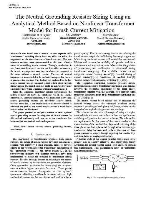
The Neutral Grounding Resistor Sizing Using an Analytical Method Based on Nonlinear Transformer Model for Inrush Current MitigationGholamabas M.H.Hajivar Shahid Chamran University,Ahvaz, Iranhajivar@S.S.MortazaviShahid Chamran University,Ahvaz, IranMortazavi_s@scu.ac.irMohsen SanieiShahid Chamran University,Ahvaz, IranMohsen.saniei@Abstract-It was found that a neutral resistor together with 'simultaneous' switching didn't have any effect on either the magnitudes or the time constant of inrush currents. The pre-insertion resistors were recommended as the most effective means of controlling inrush currents. Through simulations, it was found that the neutral resistor had little effect on reducing the inrush current peak or even the rate of decay as compared to the cases without a neutral resistor. The use of neutral impedances was concluded to be ineffective compared to the use of pre-insertion resistors. This finding was explained by the low neutral current value as compared to that of high phase currents during inrush. The inrush currents could be mitigated by using a neutral resistor when sequential switching is implemented. From the sequential energizing scheme performance, the neutral resistor size plays the significant role in the scheme effectiveness. Through simulation, it was found that a few ohms neutral grounding resistor can effectively achieve inrush currents reduction. If the neutral resistor is directly selected to minimize the peak of the actual inrush current, a much lower resistor value could be found.This paper presents an analytical method to select optimal neutral grounding resistor for mitigation of inrush current. In this method nonlinearity and core loss of the transformer has been modeled and derived analytical equations.Index Terms--Inrush current, neutral grounding resistor, transformerI.I NTRODUCTIONThe energizing of transformers produces high inrush currents. The nature of inrush currents have rich in harmonics coupled with relatively a long duration, leads to adverse effects on the residual life of the transformer, malfunction of the protection system [1] and power quality [2]. In the power-system industry, two different strategies have been implemented to tackle the problem of transformer inrush currents. The first strategy focuses on adapting to the effects of inrush currents by desensitizing the protection elements. Other approaches go further by 'over-sizing' the magnetic core to achieve higher saturation flux levels. These partial countermeasures impose downgrades on the system's operational reliability, considerable increases unit cost, high mechanical stresses on the transformer and lead to a lower power quality. The second strategy focuses on reducing the inrush current magnitude itself during the energizing process. Minimizing the inrush current will extend the transformer's lifetime and increase the reliability of operation and lower maintenance and down-time costs. Meanwhile, the problem of protection-system malfunction is eliminated during transformer energizing. The available inrush current mitigation consist "closing resistor"[3], "control closing of circuit breaker"[4],[5], "reduction of residual flux"[6], "neutral resistor with sequential switching"[7],[8],[9].The sequential energizing technique presents inrush-reduction scheme due to transformer energizing. This scheme involves the sequential energizing of the three phases transformer together with the insertion of a properly sized resistor at the neutral point of the transformer energizing side [7] ,[8],[9] (Fig. 1).The neutral resistor based scheme acts to minimize the induced voltage across the energized windings during sequential switching of each phase and, hence, minimizes the integral of the applied voltage across the windings.The scheme has the main advantage of being a simpler, more reliable and more cost effective than the synchronous switching and pre-insertion resistor schemes. The scheme has no requirements for the speed of the circuit breaker or the determination of the residual flux. Sequential switching of the three phases can be implemented through either introducing a mechanical delay between each pole in the case of three phase breakers or simply through adjusting the breaker trip-coil time delay for single pole breakers.A further study of the scheme revealed that a much lower resistor size is equally effective. The steady-state theory developed for neutral resistor sizing [8] is unable to explain this phenomenon. This phenomenon must be understood using transient analysis.Fig. 1. The sequential phase energizing schemeUPEC201031st Aug - 3rd Sept 2010The rise of neutral voltage is the main limitation of the scheme. Two methods present to control the neutral voltage rise: the use of surge arrestors and saturated reactors connected to the neutral point. The use of surge arresters was found to be more effective in overcoming the neutral voltage rise limitation [9].The main objective of this paper is to derive an analytical relationship between the peak of the inrush current and the size of the resistor. This paper presents a robust analytical study of the transformer energizing phenomenon. The results reveal a good deal of information on inrush currents and the characteristics of the sequential energizing scheme.II. SCHEME PERFORMANCESince the scheme adopts sequential switching, each switching stage can be investigated separately. For first-phase switching, the scheme's performance is straightforward. The neutral resistor is in series with the energized phase and this resistor's effect is similar to a pre-insertion resistor.The second- phase energizing is one of the most difficult to analyze. Fortunately, from simulation studies, it was found that the inrush current due to second-phase energizing is lower than that due to first-phase energizing for the same value of n R [9]. This result is true for the region where the inrush current of the first-phase is decreasing rapidly as n R increases. As a result, when developing a neutral-resistor-sizing criterion, the focus should be directed towards the analysis of the first-phase energizing.III. A NALYSIS OF F IRST -P HASE E NERGIZING The following analysis focuses on deriving an inrush current waveform expression covering both the unsaturatedand saturated modes of operation respectively. The presented analysis is based on a single saturated core element, but is suitable for analytical modelling of the single-phase transformers and for the single-phase switching of three-phase transformers. As shown in Fig. 2, the transformer's energized phase was modeled as a two segmented saturated magnetizing inductance in series with the transformer's winding resistance, leakage inductance and neutral resistance. The iron core non-l inear inductance as function of the operating flux linkages is represented as a linear inductor inunsaturated ‘‘m l ’’ and saturated ‘‘s l ’’ modes of operation respectively. (a)(b)Fig. 2. (a) Transformer electrical equivalent circuit (per-phase) referred to the primary side. (b) Simplified, two slope saturation curve.For the first-phase switching stage, the equivalent circuit represented in Fig. 2(a) can accurately represent behaviour of the transformer for any connection or core type by using only the positive sequence Flux-Current characteristics. Based on the transformer connection and core structure type, the phases are coupled either through the electrical circuit (3 single phase units in Yg-D connection) or through the Magnetic circuit (Core type transformers with Yg-Y connection) or through both, (the condition of Yg-D connection in an E-Core or a multi limb transformer). The coupling introduced between the windings will result in flux flowing through the limbs or magnetic circuits of un-energized phases. For the sequential switching application, the magnetic coupling will result in an increased reluctance (decreased reactance) for zero sequence flux path if present. The approach presented here is based on deriving an analytical expression relating the amount of inrush current reduction directly to the neutral resistor size. Investigation in this field has been done and some formulas were given to predict the general wave shape or the maximum peak current.A. Expression for magnitude of inrush currentIn Fig. 2(a), p r and p l present the total primary side resistance and leakage reactance. c R shows the total transformer core loss. Secondary side resistance sp r and leakage reactance sp l as referred to primary side are also shown. P V and s V represent the primary and secondary phase to ground terminal voltages, respectively.During first phase energizing, the differential equation describing behaviour of the transformer with saturated ironcore can be written as follows:()())sin((2) (1)φω+⋅⋅=⋅+⋅+⋅+=+⋅+⋅+=t V (t)V dtdi di d λdt di l (t)i R r (t)V dt d λdt di l (t)i R r (t)V m P ll p pp n p P p p p n p PAs the rate of change of the flux linkages with magnetizing current dt d /λcan be represented as an inductance equal to the slope of the i −λcurve, (2) can be re-written as follows;()(3) )()()(dtdi L dt di l t i R r t V lcore p p P n p P ⋅+⋅+⋅+=λ (4) )()(L core l p c l i i R dtdi−⋅=⋅λ⎩⎨⎧==sml core L L di d L λλ)(s s λλλλ>≤The general solution of the differential equations (3),(4) has the following form;⎪⎩⎪⎨⎧>−⋅⋅+−⋅+−−⋅+≤−⋅⋅+−⋅+−⋅=(5) )sin(//)()( )sin(//)(s s 22222221211112121111λλψωττλλψωττt B t e A t t e i A t B t e A t e A t i s s pSubscripts 11,12 and 21,22 denote un-saturated and saturated operation respectively. The parameters given in the equation (5) are given by;() )(/12221σ⋅++⎟⎟⎠⎞⎜⎜⎝⎛⋅−++⋅=m p c p m n p c m m x x R x x R r R x V B()2222)(/1σ⋅++⎟⎟⎠⎞⎜⎜⎝⎛⋅−++⋅=s p c p s n p c s m x x R x x R r R x V B⎟⎟⎟⎟⎟⎠⎞⎜⎜⎜⎜⎜⎝⎛⋅−+++=⋅−−⎟⎟⎟⎠⎞⎜⎜⎜⎝⎛−c p m n p m p c m R x x R r x x R x σφψ111tan tan ⎟⎟⎟⎟⎟⎠⎞⎜⎜⎜⎜⎜⎝⎛⋅−+++=⋅−−⎟⎟⎟⎠⎞⎜⎜⎜⎝⎛−c p s n p s p c m R R r x x R x σφψ112tan tan )sin(111211ψ⋅=+B A A )sin(222221s t B A A ⋅−⋅=+ωψ mp n p m p m p m p c xx R r x x x x x x R ⋅⋅+⋅−⋅+−⋅+⋅⋅⋅=)(4)()(21211σστm p n p m p m p m p c xx R r x x x x x x R ⋅⋅+⋅−⋅++⋅+⋅⋅⋅=)(4)()(21212σστ s p n p s p s p s p xx R r x x x x x x c R ⋅⋅+⋅−⋅+−⋅+⋅⋅⋅=)(4)()(21221σστ sp n p s p s p sp c xx R r x x x x x x R ⋅⋅+⋅−⋅++⋅+⋅⋅⋅=)(4)()(21222σστ ⎟⎟⎠⎞⎜⎜⎝⎛−⋅==s rs s ri i λλλ10 cnp R R r ++=1σ21221112 , ττττ>>>>⇒>>c R , 012≈A , 022≈A According to equation (5), the required inrush waveform assuming two-part segmented i −λcurve can be calculated for two separate un-saturated and saturated regions. For thefirst unsaturated mode, the current can be directly calculated from the first equation for all flux linkage values below the saturation level. After saturation is reached, the current waveform will follow the second given expression for fluxlinkage values above the saturation level. The saturation time s t can be found at the time when the current reaches the saturation current level s i .Where m λ,r λ,m V and ωare the nominal peak flux linkage, residual flux linkage, peak supply voltage and angular frequency, respectivelyThe inrush current waveform peak will essentially exist during saturation mode of operation. The focus should be concentrated on the second current waveform equation describing saturated operation mode, equation (5). The expression of inrush current peak could be directly evaluated when both saturation time s t and peak time of the inrush current waveform peak t t =are known [9].(10))( (9) )(2/)(222222121//)()(2B eA t e i A peak peak t s t s n peak n n peak R I R R t +−⋅+−−⋅+=+=ττωψπThe peak time peak t at which the inrush current will reachits peak can be numerically found through setting the derivative of equation (10) with respect to time equal to zero at peak t t =.()(11) )sin(/)(022222221212221/ψωωττττ−⋅⋅⋅−−−⋅+−=+−⋅peak t s t B A t te A i peak s peakeThe inrush waveform consists of exponentially decaying'DC' term and a sinusoidal 'AC' term. Both DC and AC amplitudes are significantly reduced with the increase of the available series impedance. The inrush waveform, neglecting the relatively small saturating current s i ,12A and 22A when extremely high could be normalized with respect to theamplitude of the sinusoidal term as follows; (12) )sin(/)()(2221221⎥⎦⎤⎢⎣⎡−⋅+−−⋅⋅=ψωτt t t e B A B t i s p(13) )sin(/)()sin()( 22221⎥⎦⎤⎢⎣⎡−⋅+−−⋅⋅−⋅=ψωτωψt t t e t B t i s s p ))(sin()( 2s n n t R R K ⋅−=ωψ (14) ωλλλφλφωλλφωmm m r s s t r m s mV t dt t V dtd t V V s=⎪⎭⎪⎬⎫⎪⎩⎪⎨⎧⎥⎥⎦⎤⎢⎢⎣⎡⎟⎟⎠⎞⎜⎜⎝⎛−−+−⋅=+⋅+⋅⋅==+⋅⋅=−∫(8) 1cos 1(7))sin((6))sin(10The factor )(n R K depends on transformer saturation characteristics (s λand r λ) and other parameters during saturation.Typical saturation and residual flux magnitudes for power transformers are in the range[9]; .).(35.1.).(2.1u p u p s <<λ and .).(9.0.).(7.0u p r u p <<λIt can be easily shown that with increased damping 'resistance' in the circuit, where the circuit phase angle 2ψhas lower values than the saturation angle s t ⋅ω, the exponential term is negative resulting in an inrush magnitude that is lowerthan the sinusoidal term amplitude.B. Neutral Grounding Resistor SizingBased on (10), the inrush current peak expression, it is now possible to select a neutral resistor size that can achieve a specific inrush current reduction ratio )(n R α given by:(15) )0(/)()(==n peak n peak n R I R I R α For the maximum inrush current condition (0=n R ), the total energized phase system impedance ratio X/R is high and accordingly, the damping of the exponential term in equation (10) during the first cycle can be neglected; [][](16))0(1)0()0(2212=⋅++⎥⎦⎤⎢⎣⎡⋅−+===⎟⎟⎠⎞⎜⎜⎝⎛+⋅⋅n s p c p s pR x n m n peak R x x R x x r R K V R I c s σ High n R values leading to considerable inrush current reduction will result in low X / R ratios. It is clear from (14) that X / R ratios equal to or less than 1 ensure negative DC component factor ')(n R K ' and hence the exponential term shown in (10) can be conservatively neglected. Accordingly, (10) can be re-written as follows;()[](17) )()(22122n s p c p s n p R x m n n peak R x x R x x R r V R B R I c s σ⋅++⎥⎦⎤⎢⎣⎡⋅−+=≈⎟⎟⎠⎞⎜⎜⎝⎛+⋅Using (16) and (17) to evaluate (15), the neutral resistorsize which corresponds to a specific reduction ratio can be given by;[][][](18) )0()(1)0( 12222=⋅++⋅−⋅++⋅−+⋅+=⎥⎥⎦⎤⎢⎢⎣⎡⎥⎥⎦⎤⎢⎢⎣⎡=n s p c p s p n s p c p s n p n R x x R x x r R x x R x x R r R K σσα Very high c R values leading to low transformer core loss, it can be re-written equation (18) as follows [9]; [][][][](19) 1)0(12222s p p s p n p n x x r x x R r R K +++++⋅+==α Equations (18) and (19) reveal that transformers require higher neutral resistor value to achieve the desired inrush current reduction rate. IV. A NALYSIS OF SECOND-P HASE E NERGIZING It is obvious that the analysis of the electric and magnetic circuit behavior during second phase switching will be sufficiently more complex than that for first phase switching.Transformer behaviour during second phase switching was served to vary with respect to connection and core structure type. However, a general behaviour trend exists within lowneutral resistor values where the scheme can effectively limitinrush current magnitude. For cases with delta winding or multi-limb core structure, the second phase inrush current is lower than that during first phase switching. Single phase units connected in star/star have a different performance as both first and second stage inrush currents has almost the same magnitude until a maximum reduction rate of about80% is achieved. V. NEUTRAL VOLTAGE RISEThe peak neutral voltage will reach values up to peak phasevoltage where the neutral resistor value is increased. Typicalneutral voltage peak profile against neutral resistor size is shown in Fig. 6- Fig. 8, for the 225 KVA transformer during 1st and 2nd phase switching. A del ay of 40 (ms) between each switching stage has been considered. VI. S IMULATION A 225 KVA, 2400V/600V, 50 Hz three phase transformer connected in star-star are used for the simulation study. The number of turns per phase primary (2400V) winding is 128=P N and )(01.0pu R R s P ==, )(05.0pu X X s P ==,active power losses in iron core=4.5 KW, average length and section of core limbs (L1=1.3462(m), A1=0.01155192)(2m ), average length and section of yokes (L2=0.5334(m),A2=0.01155192)(2m ), average length and section of air pathfor zero sequence flux return (L0=0.0127(m),A0=0.01155192)(2m ), three phase voltage for fluxinitialization=1 (pu) and B-H characteristic of iron core is inaccordance with Fig.3. A MATLAB program was prepared for the simulation study. Simulation results are shown in Fig.4-Fig.8.Fig. 3.B-H characteristic iron coreFig.4. Inrush current )(0Ω=n RFig.5. Inrush current )(5Ω=n RFig.6. Inrush current )(50Ω=n RFig.7. Maximum neutral voltage )(50Ω=n RFig.8. Maximum neutral voltage ).(5Ω=n RFig.9. Maximum inrush current in (pu), Maximum neutral voltage in (pu), Duration of the inrush current in (s)VII. ConclusionsIn this paper, Based on the sequential switching, presents an analytical method to select optimal neutral grounding resistor for transformer inrush current mitigation. In this method, complete transformer model, including core loss and nonlinearity core specification, has been used. It was shown that high reduction in inrush currents among the three phases can be achieved by using a neutral resistor .Other work presented in this paper also addressed the scheme's main practical limitation: the permissible rise of neutral voltage.VIII.R EFERENCES[1] Hanli Weng, Xiangning Lin "Studies on the UnusualMaloperation of Transformer Differential Protection During the Nonlinear Load Switch-In",IEEE Transaction on Power Delivery, vol. 24, no.4, october 2009.[2] Westinghouse Electric Corporation, Electric Transmissionand Distribution Reference Book, 4th ed. East Pittsburgh, PA, 1964.[3] K.P.Basu, Stella Morris"Reduction of Magnetizing inrushcurrent in traction transformer", DRPT2008 6-9 April 2008 Nanjing China.[4] J.H.Brunke, K.J.Frohlich “Elimination of TransformerInrush Currents by Controlled Switching-Part I: Theoretical Considerations” IEEE Trans. On Power Delivery, Vol.16,No.2,2001. [5] R. Apolonio,J.C.de Oliveira,H.S.Bronzeado,A.B.deVasconcellos,"Transformer Controlled Switching:a strategy proposal and laboratory validation",IEEE 2004, 11th International Conference on Harmonics and Quality of Power.[6] E. Andersen, S. Bereneryd and S. Lindahl, "SynchronousEnergizing of Shunt Reactors and Shunt Capacitors," OGRE paper 13-12, pp 1-6, September 1988.[7] Y. Cui, S. G. Abdulsalam, S. Chen, and W. Xu, “Asequential phase energizing method for transformer inrush current reduction—part I: Simulation and experimental results,” IEEE Trans. Power Del., vol. 20, no. 2, pt. 1, pp. 943–949, Apr. 2005.[8] W. Xu, S. G. Abdulsalam, Y. Cui, S. Liu, and X. Liu, “Asequential phase energizing method for transformer inrush current reduction—part II: Theoretical analysis and design guide,” IEEE Trans. Power Del., vol. 20, no. 2, pt. 1, pp. 950–957, Apr. 2005.[9] S.G. Abdulsalam and W. Xu "A Sequential PhaseEnergization Method for Transformer Inrush current Reduction-Transient Performance and Practical considerations", IEEE Transactions on Power Delivery,vol. 22, No.1, pp. 208-216,Jan. 2007.。
90-A geometric setting for the quantum deformation of GLn

DUKE MATHEMATICAL JOURNAL (C)
October 1990
A GEOMETRIC SETTING FOR THE QUANTUM DEFORMATION OF GL
A. A. BEILINSON, G. LUSZTIG*,
AND
R. MACPHERSON*
1. Flags and the algebra K. 1.1. We fix an integer n>l. Let i9 be the set of all n n matrices with integer entries such that the entries off diagonal are > 0. Let (R) be the set of all n x n matrices with integer, > 0 entries. Thus, (R) c 19. Let r: 19 ---, N be the map defined by taking the sum of all entries of a matrix. Let (R)a a-l(d); we have (R) Ila>o (R)a, and each (R)a is a finite set. Let V be a vector space of finite dimension d over a field F. Let be the set of all n-step filtrations V1 c V2 c"" V. E The group GL(V) acts naturally on -; its orbits are the fibres of the map --, N" given by
LucasKanadeMeetsHornSchunckCombiningLocaland GlobalOptic

International Journal of Computer Vision61(3),211–231,2005c 2005Springer Science+Business Media,Inc.Manufactured in The Netherlands. Lucas/Kanade Meets Horn/Schunck:Combining Local and Global OpticFlow MethodsANDR´ES BRUHN AND JOACHIM WEICKERTMathematical Image Analysis Group,Faculty of Mathematics and Computer Science,Saarland University,Building27,66041Saarbr¨u cken,Germanybruhn@mia.uni-saarland.deweickert@mia.uni-saarland.deCHRISTOPH SCHN¨ORRComputer Vision,Graphics and Pattern Recognition Group,Faculty of Mathematics and Computer Science,University of Mannheim,68131Mannheim,Germanyschnoerr@uni-mannheim.deReceived August5,2003;Revised April22,2004;Accepted April22,2004First online version published in October,2004Abstract.Differential methods belong to the most widely used techniques for opticflow computation in image sequences.They can be classified into local methods such as the Lucas–Kanade technique or Big¨u n’s structure tensor method,and into global methods such as the Horn/Schunck approach and its extensions.Often local methods are more robust under noise,while global techniques yield denseflowfields.The goal of this paper is to contribute to a better understanding and the design of novel differential methods in four ways:(i)We juxtapose the role of smoothing/regularisation processes that are required in local and global differential methods for opticflow computation.(ii)This discussion motivates us to describe and evaluate a novel method that combines important advantages of local and global approaches:It yields denseflowfields that are robust against noise.(iii)Spatiotemporal and nonlinear extensions as well as multiresolution frameworks are presented for this hybrid method.(iv)We propose a simple confidence measure for opticflow methods that minimise energy functionals.It allows to sparsify a dense flowfield gradually,depending on the reliability required for the resultingflparisons with experiments from the literature demonstrate the favourable performance of the proposed methods and the confidence measure. Keywords:opticflow,differential techniques,variational methods,structure tensor,partial differential equations, confidence measures,performance evaluation1.IntroductionIll-posedness is a problem that is present in many im-age processing and computer vision techniques:Edgedetection,for example,requires the computation of im-age derivatives.This problem is ill-posed in the senseof Hadamard,1as small perturbations in the signalmay create largefluctuations in its derivatives(Yuilleand Poggio,1986).Another example consists of opticflow computation,where the ill-posedness manifestsitself in the nonuniqueness due to the aperture prob-lem(Bertero et al.,1988):The data allow to computeonly the opticflow component normal to image edges.Both types of ill-posedness problems appear jointlyin so-called differential methods for opticflow recov-ery,where opticflow estimation is based on computing212Bruhn,Weickert and Schn¨o rrspatial and temporal image derivatives.These tech-niques can be classified into local methods that may optimise some local energy-like expression,and global strategies which attempt to minimise a global en-ergy functional.Examples of thefirst category include the Lucas–Kanade method(Lucas and Kanade,1981; Lucas,1984)and the structure tensor approach of Big¨u n and Granlund(1988)and Big¨u n et al.(1991), while the second category is represented by the clas-sic method of Horn and Schunck(Horn and Schunck, 1981)and its numerous discontinuity-preserving vari-ants(Alvarez et al.,1999;Aubert et al.,1999;Black and Anandan,1991;Cohen,1993;Heitz and Bouthemy, 1993;Kumar et al.,1996;Nagel,1983;Nesi,1993; Proesmans et al.,1994;Schn¨o rr,1994;Shulman and Herv´e,1989;Weickert and Schn¨o rr,2001).Differential methods are rather popular:Together with phase-based methods such as(Fleet and Jepson,1990)they belong to the techniques with the best performance(Barron et al.,1994;Galvin et al.,1998).Local methods may offer relatively high robustness under noise,but do not give denseflowfields.Global methods,on the other hand, yieldflowfields with100%density,but are experimen-tally known to be more sensitive to noise(Barron et al., 1994;Galvin et al.,1998).A typical way to overcome the ill-posedness prob-lems of differential opticflow methods consists of the use of smoothing techniques and smoothness as-sumptions:It is common to smooth the image se-quence prior to differentiation in order to remove noise and to stabilise the differentiation process.Lo-cal techniques use spatial constancy assumptions on the opticflowfield in the case of the Lucas–Kanade method,and spatiotemporal constancy for the Big¨u n method.Global approaches,on the other hand,sup-plement the opticflow constraint with a regularising smoothness term.Surprisingly,the actual role and the difference between these smoothing strategies,how-ever,has hardly been addressed in the literature so far. In afirst step of this paper we juxtapose the role of the different smoothing steps of these methods.We shall see that each smoothing process offers certain advantages that cannot be found in other cases.Conse-quently,it would be desirable to combine the different smoothing effects of local and global methods in or-der to design novel approaches that combine the high robustness of local methods with the full density of global techniques.One of the goals of the present pa-per is to propose and analyse such an embedding of local methods into global approaches.This results in a technique that is robust under noise and givesflow fields with100%density.Hence,there is no need for a postprocessing step where sparse data have to be interpolated.On the other hand,it has sometimes been criticised that there is no reliable confidence measure that al-lows to sparsify the result of a denseflowfield such that the remainingflow is more reliable(Barron et al., 1994).In this way it would be possible to compare the real quality of dense methods with the character-istics of local,nondense approaches.In our paper we shall present such a measure.It is simple and applica-ble to the entire class of energy minimising global op-ticflow techniques.Our experimental evaluation will show that this confidence measure can give excellent results.Our paper is organised as follows.In Section2 we discuss the role of the different smoothing pro-cesses that are involved in local and global opticflow approaches.Based on these results we propose two combined local-global(CLG)methods in Section3, one with spatial,the other one with spatiotemporal smoothing.In Section4nonlinear variants of the CLG method are presented,while a suitable multiresolu-tion framework is discussed in Section5.Our nu-merical algorithm is described in Section6.In Sec-tion7,we introduce a novel confidence measure for all global opticflow methods that use energy func-tionals.Section8is devoted to performance evalua-tions of the CLG methods and the confidence mea-sure.A summary and an outlook to future work is given in Section9.In the Appendix,we show how the CLG principle has to be modified if one wants to replace the Lucas–Kanade method by the struc-ture tensor method of Big¨u n and Granlund(1988)and Big¨u n et al.(1991).1.1.Related WorkIn spite of the fact that there exists a very large number of publications on motion analysis(see e.g.(Mitiche and Bouthemy,1996;Stiller and Konrad,1999)for reviews),there has been remarkably little work de-voted to the integration of local and global opticflow methods.Schn¨o rr(Schn¨o rr,1993)sketched a frame-work for supplementing global energy functionals with multiple equations that provide local data constraints. He suggested to use the output of Gaussianfilters shifted in frequency space(Fleet and Jepson,1990)orLucas/Kanade Meets Horn/Schunck213local methods incorporating second-order derivatives (Tretiak and Pastor,1984;Uras et al.,1988),but did not consider methods of Lucas–Kanade or Big¨u n type. Our proposed technique differs from the majority of global regularisation methods by the fact that we also use spatiotemporal regularisers instead of spa-tial ones.Other work with spatiotemporal regularisers includes publications by Murray and Buxton(1987), Nagel(1990),Black and Anandan(1991),Elad and Feuer(1998),and Weickert and Schn¨o rr(2001). While the noise sensitivity of local differential methods has been studied intensively in recent years (Bainbridge-Smith and Lane,1997;Ferm¨u ller et al., 2001;J¨a hne,2001;Kearney et al.,1987;Ohta,1996; Simoncelli et al.,1991),the noise sensitivity of global differential methods has been analysed to a signifi-cantly smaller extent.In this context,Galvin et al. (1998)have compared a number of classical methods where small amounts of Gaussian noise had been added.Their conclusion was similar to thefindings of Barron et al.(1994):the global approach of Horn and Schunck is more sensitive to noise than the local Lucas–Kanade method.A preliminary shorter version of the present paper has been presented at a conference(Bruhn et al.,2002). Additional work in the current paper includes(i)the use of nonquadratic penalising functions,(ii)the ap-plication of a suitable multiresolution strategy,(iii)the proposal of a confidence measure for the entire class of global variational methods,(iv)the integration of the structure tensor approach of Big¨u n and Granlund (1988)and Big¨u n et al.(1991)and(v)a more extensive experimental evaluation.2.Role of the Smoothing ProcessesIn this section we discuss the role of smoothing tech-niques in differential opticflow methods.For simplicity we focus on spatial smoothing.All spatial smoothing strategies can easily be extended into the temporal domain.This will usually lead to improved results (Weickert and Schn¨o rr,2001).Let us consider some image sequence g(x,y,t), where(x,y)denotes the location within a rectangular image domain ,and t∈[0,T]denotes time.It is com-mon to smooth the image sequence prior to differentia-tion(Barron et al.,1994;Kearney et al.,1987),e.g.by convolving each frame with some Gaussian Kσ(x,y) of standard deviationσ:f(x,y,t):=(Kσ∗g)(x,y,t),(1)The low-pass effect of Gaussian convolution removes noise and other destabilising high frequencies.In a sub-sequent opticflow method,we may thus callσthe noise scale.Many differential methods for opticflow are based on the assumption that the grey values of image objects in subsequent frames do not change over time:f(x+u,y+v,t+1)=f(x,y,t),(2) where the displacementfield(u,v) (x,y,t)is called opticflow.For small displacements,we may perform afirst order Taylor expansion yielding the opticflow constraintf x u+f y v+f t=0,(3) where subscripts denote partial derivatives.Evidently, this single equation is not sufficient to uniquely com-pute the two unknowns u and v(aperture problem): For nonvanishing image gradients,it is only possible to determine theflow component parallel to∇f:= (f x,f y) ,i.e.normal to image edges.This so-called normalflow is given byw n=−f t∇f.(4)Figure1(a)depicts one frame from the famous Hamburg taxi sequence.2We have added Gaussian noise,and in Fig.1(b)–(d)we illustrate the impact of presmoothing the image data on the normalflow. While some moderate presmoothing improves the re-sults,great care should be taken not to apply too much presmoothing,since this would severely destroy im-portant image structure.In order to cope with the aperture problem,Lucas and Kanade(1981)and Lucas(1984)proposed to assume that the unknown opticflow vector is constant within some neighbourhood of sizeρ.In this case it is possible to determine the two constants u and v at some location (x,y,t)from a weighted least squarefit by minimising the functionE L K(u,v):=Kρ∗(f x u+f y v+f t)2.(5) Here the standard deviationρof the Gaussian serves as an integration scale over which the main contribution of the least squarefit is computed.A minimum(u,v)of E L K satisfies∂u E L K=0and ∂v E L K=0.This gives the linear systemKρ∗f2xKρ∗(f x f y)Kρ∗(f x f y)Kρ∗f2yuv=−Kρ∗(f x f t)−Kρ∗(f y f t)(6)214Bruhn,Weickert and Schn¨orrFigure 1.From left to right,and from top to bottom :(a)Frame 10of the Hamburg taxi sequence,where Gaussian noise with standard deviationσn =10has been added.The white taxi turns around the corner,the left car drives to the right,and the right van moves to the left.(b)Normal flow magnitude without presmoothing.(c)Normal flow magnitude,presmoothing with σ=1.(d)Ditto,presmoothing with σ=5.(e)Lucas-Kanade method with σ=0,ρ=7.5.(f)Ditto,σ=0,ρ=15.(g)Optic flow magnitude with the Horn-Schunck approach,σ=0,α=105.(h)Ditto,σ=0,α=106.which can be solved provided that its system matrix is invertible.This is not the case in flat regions where the image gradient vanishes.In some other regions,the smaller eigenvalue of the system matrix may be close to 0,such that the aperture problem remains present and the data do not allow a reliable determination of the full optic flow.All this results in nondense flow fields.They constitute the most severe drawback of local gradient methods:Since many computer vision applications require dense flow estimates,subsequent interpolation steps are needed.On the other hand,one may use the smaller eigenvalue of the system matrix as a confidence measure that characterises the reliability of the estimate.Experiments by Barron et al.(1994)indicated that this performs better than the trace-based confidence measure in Simoncelli et al.(1991).Figure 1(e)and (f)show the influence of the integra-tion scale ρon the final result.In these images we haveLucas/Kanade Meets Horn/Schunck215 displayed the entireflowfield regardless of its localreliability.We can see that in each case,theflowfieldhas typical structures of orderρ.In particular,a suffi-ciently large value forρis very successful in renderingthe Lucas–Kanade method robust under noise.In order to end up with denseflow estimates one mayembed the opticflow constraint into a regularisationframework.Horn and Schunck(Horn and Schunck,1981)have pioneered this class of global differen-tial methods.They determine the unknown functionsu(x,y,t)and v(x,y,t)as the minimisers of the globalenergy functionalE HS(u,v)=((f x u+f y v+f t)2+α(|∇u|2+|∇v|2))dx dy(7)where the smoothness weightα>0serves as regu-larisation parameter:Larger values forαresult in astronger penalisation of largeflow gradients and leadto smootherflowfields.Minimising this convex functional comes down tosolving its corresponding Euler–Lagrange equations(Courant and Hilbert,1953;Elsgolc,1961).They aregiven by0= u−1αf2x u+f x f y v+f x f t,(8)0= v−1f x f y u+f2y v+f y f t.(9)with reflecting boundary conditions. denotes the spa-tial Laplace operator::=∂xx+∂yy.(10) The solution of these diffusion–reaction equations is not only unique(Schn¨o rr,1991),it also benefits from thefilling-in effect:At locations with|∇f|≈0,no reliable localflow estimate is possible,but the reg-ulariser|∇u|2+|∇v|2fills in information from theneighbourhood.This results in denseflowfields and makes subsequent interpolation steps obsolete.This is a clear advantage over local methods.It has,however,been criticised that for such global differential methods,no good confidence measures are available that would help to determine locations where the computations are more reliable than elsewhere (Barron et al.,1994).It has also been observed that they may be more sensitive to noise than local differential methods(Barron et al.,1994;Galvin et al.,1998).An explanation for this behaviour can be given as follows.Noise results in high image gradients.They serve as weights in the data term of the regularisation functional(7).Since the smoothness term has a con-stant weightα,smoothness is relatively less important at locations with high image gradients than elsewhere. As a consequence,flowfields are less regularised at noisy image structures.This sensitivity under noise is therefore nothing else but a side-effect of the desired filling-in effect.Figure1(g)and(h)illustrate this be-haviour.Figure1(g)shows that theflowfield does not reveal a uniform scale:It lives on afine scale at high gra-dient image structures,and the scale may become very large when the image gradient tends to zero.Increasing the regularisation parameterαwillfinally also smooth theflowfield at noisy structures,but at this stage,it might already be too blurred inflatter image regions (Fig.1(h)).3.A Combined Local–Global MethodWe have seen that both local and global differential methods have complementary advantages and short-comings.Hence it would be interesting to construct a hybrid technique that constitutes the best of two worlds:It should combine the robustness of local methods with the density of global approaches.This shall be done next.We start with spatial formulations before we extend the approach to the spatiotemporal domain.3.1.Spatial ApproachIn order to design a combined local–global(CLG) method,let usfirst reformulate the previous ing the notationsw:=(u,v,1) ,(11)|∇w|2:=|∇u|2+|∇v|2,(12)∇3f:=(f x,f y,f t) ,(13) Jρ(∇3f):=Kρ∗(∇3f∇3f )(14)it becomes evident that the Lucas–Kanade method min-imises the quadratic formE L K(w)=w Jρ(∇3f)w,(15)216Bruhn,Weickert and Schn¨o rrwhile the Horn–Schunck technique minimises the functionalE HS(w)=(w J0(∇3f)w+α|∇w|2)dx dy.(16)This terminology suggests a natural way to extend the Horn–Schunck functional to the desired CLG func-tional.We simply replace the matrix J0(∇3f)by the structure tensor Jρ(∇3f)with some integration scale ρ>0.Thus,we propose to minimise the functionalE CLG(w)=w Jρ(∇3f)w+α|∇w|2dx dy.(17)Its minimisingflowfield(u,v)satisfies the Euler–Lagrange equations0= u−1αKρ∗f2xu+Kρ∗(f x f y)v+Kρ∗(f x f t),(18)0= v−1Kρ∗(f x f y)u+Kρ∗f2yv+Kρ∗(f y f t).(19)It should be noted that these equations are hardly more complicated than the original Horn–Schunck Eqs.(8) and(9).All one has to do is to evaluate the terms con-taining image data at a nonvanishing integration scale. The basic structure with respect to the unknown func-tions u(x,y,t)and v(x,y,t)is identical.It is there-fore not surprising that the well-posedness proof for the Horn–Schunck method that was presented in(Schn¨o rr, 1991)can also be extended to this case.3.2.Spatiotemporal ApproachThe previous approaches used only spatial smooth-ness operators.Rapid advances in computer technol-ogy,however,makes it now possible to consider also spatiotemporal smoothness operators.Formal exten-sions in this direction are straightforward.In general, one may expect that spatiotemporal formulations give better results than spatial ones because of the additional denoising properties along the temporal direction.In the presence of temporalflow discontinuities smooth-ing along the time axis should only be used moderately. However,even in this case one can observe the benefi-cial effect of temporal information.A spatiotemporal variant of the Lucas–Kanade ap-proach simply replaces convolution with2-D Gaus-sians by spatiotemporal convolution with3-D Gaus-sians.This still leads to a2×2linear system of equa-tions for the two unknowns u and v. Spatiotemporal versions of the Horn-Schunck method have been considered by Elad and Feuer (1998),while discontinuity preserving global methods with spatiotemporal regularisers have been proposed in different formulations in Black and Anandan(1991), Murray and Buxton(1987),Nagel(1990),Weickert and Schn¨o rr(2001).Combining the temporal extended variant of both the Lucas–Kanade and the Horn–Schunck method we obtain a spatiotemporal version of our CLG functional given byE C LG3(w)=×[0,T](w Jρ(∇3f)w+α|∇3w|2)dx dy dt(20) where convolutions with Gaussians are now to be un-derstood in a spatiotemporal way and|∇3w|2:=|∇3u|2+|∇3v|2.(21)Due to the different role of space and time the spa-tiotemporal Gaussians may have different standard de-viations in both directions.Let us denote by J nm the component(n,m)of the structure tensor Jρ(∇3f). Then the Euler–Lagrange equations for(20)are given by3u−1α(J11u+J12v+J13)=0,(22) 3v−1(J12u+J22v+J23)=0.(23)One should note that they have the same structure as(18)–(19),apart from the fact that spatiotempo-ral Gaussian convolution is used,and that the spa-tial Laplacean is replaced by the spatiotemporal Laplacean3:=∂xx+∂yy+∂tt.(24)The spatiotemporal Lucas–Kanade method is similar to the approach of Big¨u n and Granlund(1988)and Big¨u n et al.(1991).In the Appendix we show how the latter method can be embedded in a global energy functional.Lucas/Kanade Meets Horn/Schunck217 4.Nonquadratic ApproachSo far the underlying Lucas–Kanade and Horn–Schunck approaches are linear methods that are basedon quadratic optimisation.It is possible to replacethem by nonquadratic optimisation problems that leadto nonlinear methods.From a statistical viewpointthis can be regarded as applying methods from ro-bust statistics where outliers are penalised less severelythan in quadratic approaches(Hampel et al.,1986;Huber,1981).In general,nonlinear methods give bet-ter results at locations withflow discontinuities.Ro-bust variants of the Lucas–Kanade method have beeninvestigated by Black and Anandan(1996)and byYacoob and Davis(1999),respectively,while a surveyof the numerous convex discontinuity-preserving reg-ularisers for global opticflow methods is presented inWeickert and Schn¨o rr(2001).In order to render our approach more robust againstoutliers in both the data and the smoothness term wepropose the minimisation of the following functional:E CLG3−N(w)=×[0,T](ψ1(w Jρ(∇3f)w)+αψ2(|∇3w|2))dx dy dt(25)whereψ1(s2)andψ2(s2)are nonquadratic penalisers.Encouraging experiments with related continuous en-ergy functionals have been performed by Hinterbergeret al.(2002).Suitable nonquadratic penalisers can bederived from nonlinear diffusionfilter design,wherepreservation or enhancement of discontinuities is alsodesired(Weickert,1998).In order to guarantee well–posedness for the remaining problem,we focus onlyon penalisers that are convex in s.In particular,we usea function that has been proposed by Charbonnier et al.(1994):ψi(s2)=2β2i1+s2i,i∈1,2(26)whereβ1andβ2are scaling parameters.Under some technical requirements,the choice of convex penalis-ers ensures a unique solution of the minimisation prob-lem and allows to construct simple globally convergent algorithms.The Euler–Lagrange equations of the energy func-tional(25)are given by0=div(ψ 2(|∇3w|2)∇3u)−1ψ 1(w Jρ(∇3f)w)(J11u+J12v+J13),(27) 0=div(ψ 2(|∇3w|2)∇3v)−1ψ 1(w Jρ(∇3f)w)(J21v+J22u+J23).(28) withψ i(s2)=11+s2β2i,i∈1,2(29)One should note that for large values ofβi the nonlinearcase comes down to the linear one sinceψi(s2)≈ 1.5.Multiresolution ApproachAll variants of the CLG method considered so far are based on a linearisation of the grey value con-stancy assumption.As a consequence,u and v are re-quired to be relatively small so that the linearisation holds.Obviously,this cannot be guaranteed for arbi-trary sequences.However,there are strategies that al-low to overcome this limitation.These so called multi-scale focusing or multiresolution techniques(Ananden, 1989;Black and Anandan,1996;M´e min and P´e rez, 1998;M´e min and P´e rez,2002)incrementally compute the opticflowfield based on a sophisticated coarse-to-fine strategy:Starting from a coarse scale the resolution is refined step by step.However,the estimatedflowfield at a coarser level is not used as initalisation at the nextfiner scale.In particular for energy functionals with a global minimum,such a proceeding would only lead to an ac-celeration of the convergence,since the result would not change.Instead,the coarse scale motion is used to warp(correct)the original sequence before going to the nextfiner level.This compensation for the already computed motion results in a hierarchy of modified problems that only require to compute small displace-mentfields,the so called motion increments.Thus it is not surprising that thefinal displacementfield obtained by a summation of all motion increments is much more accurate regarding the linearisation of the grey value constancy assumption.218Bruhn,Weickert and Schn¨o rrLet δw m denote the motion increment at resolutionlevel m ,where m =0is the coarsest level with ini-talisation w 0=(0,0,0) .Then δw m is obtained by optimisation of the following spatiotemporal energy functional:E m CLG3−N (δw m )= ×[0,T ](ψ1(δw m J ρ(∇3f (x +w m ))δw m )+αψ2(|∇3(w m +δw m )|2))dxwhere w m +1=w m +δw m and x =(x ,y ,t ).One shouldnote that warping the original sequence does only af-fect the data term.Since the smoothness assumption applies to the complete flow field,w m +δw m is used as argument of the penaliser.If we denote the structure tensor of the corrected se-quence by J mρ=J ρ(∇3f (x +w m )),the corresponding Euler–Lagrange equations are given by0=div (ψ2(|∇3(w m +δw m )|2)∇3δu m )−1αψ 1 δw m J m ρδw J m 11δu +J m 12δv +J m13,(30)0=div (ψ2(|∇3(w m +δw m )|2)∇3δv m )−1αψ 1 δw m J m ρδw J m 21δv +J m 22δu +J m23.(31)6.Algorithmic Realisation 6.1.Spatial and Spatiotemporal ApproachLet us now discuss a suitable algorithm for the CLG method (18)and (19)and its spatiotemporal variant.To this end we consider the unknown functions u (x ,y ,t )and v (x ,y ,t )on a rectangular pixel grid of size h ,and we denote by u i the approximation to u at some pixel i with i =1,...,N .Gaussian convolution is realised in the spatial/spatiotemporal domain by discrete con-volution with a truncated and renormalised Gaussian,where the truncation took place at 3times the stan-dard deviation.Symmetry and separability has been exploited in order to speed up these discrete convolu-tions.Spatial derivatives of the image data have been approximated using a sixth-order approximation with the stencil (−1,9,−45,0,45,−9,1)/(60h ).Tempo-ral derivatives are either approximated with a sim-ple two-point stencil or the fifth-order approximation(−9,125,−2250,2250,−125,9)/(1920h ).Let us denote by J nmi the component (n ,m )of the structure tensor J ρ(∇f )in some pixel i .Furthermore,let N (i )denote the set of (4in 2-D,6in 3-D)neigh-bours of pixel i .Then a finite difference approxima-tion to the Euler–Lagrange equations (18)–(19)is given by0= j ∈N (i )u j −u i h 2−1(J 11i u i +J 12i v i +J 13i ),(32)0= j ∈N (i )v j −v i h 2−1α(J 21i u i +J 22i v i +J 23i )(33)for i =1,...,N .This sparse linear system of equationsmay be solved iteratively.The successive overrelax-ation (SOR)method (Young,1971)is a good compro-mise between simplicity and efficiency.If the upper index denotes the iteration step,the SOR method can be written asu k +1i =(1−ω)u k i +ωj ∈N −(i )u k +1j + j ∈N +(i )u k j −h 2αJ 12i v k i +J 13i|N (i )|+h 2αJ 11i,(34)v k +1i =(1−ω)v k i +ωj ∈N −(i )v k +1j + j ∈N +(i )v k j −h 2αJ 21i u k +1i+J 23i|N (i )|+h αJ 22i(35)whereN −(i ):={j ∈N (i )|j <i },(36)N +(i ):={j ∈N (i )|j >i }(37)and |N (i )|denotes the number of neighbours of pixel i that belong to the image domain.The relaxation parameter ω∈(0,2)has a strong influence on the convergence speed.For ω=1one obtains the well-known Gauß–Seidel method .We usu-ally use values for ωbetween 1.9and 1.99.This nu-merically inexpensive overrelaxation step results in a speed-up by one order of magnitude compared with the Gauß–Seidel approach.We initialised the flow compo-nents for the first iteration by 0.The specific choice。
Distributed interactive simulation for group-distance exercise on the web

DISTRIBUTED INTERACTIVE SIMULATION FOR GROUP-DISTANCEEXERCISES ON THE WEBErik Berglund and Henrik ErikssonDepartment of Computer and Information ScienceLinköping UniversityS-581 83 Linköping, SwedenE-mail: {eribe, her}@ida.liu.seKEYWORDS: Distributed Interactive Simulation, Distance Education, Network, Internet, Personal ComputerABSTRACTIn distributed-interactive simulation (DIS), simulators act as elements of a bigger distributed simulation. A group-distance exercise (GDE) based on the DIS approach can therefore enable group training for group members participating from different locations. Our GDE approach, unlike full-scale DIS systems, uses affordable simulators designed for standard hardware available in homes and offices.ERCIS (group distance exERCISe) is a prototype GDE system that we have implemented. It takes advantage of Internet and Java to provide distributed simulation at a fraction of the cost of full-scale DIS systems.ERCIS illustrates that distributed simulation can bring advanced training to office and home computers in the form of GDE systems.The focus of this paper is to discuss the possibilities and the problems of GDE and of web-based distributed simulation as a means to provide GDE. INTRODUCTIONSimulators can be valuable tools in education. Simulators can reduce the cost of training and can allow training in hazardous situations (Berkum & Jong 1991). Distributed-interactive simulation (DIS) originated in military applications, where simulators from different types of forces were connected to form full battle situations. In DIS, individual simulators act as elements of a bigger distributed simulation (Loper & Seidensticker 1993).Thus, DIS could be used to create a group-distance exercise (GDE), where the participants perform a group exercise from different locations. Even though DIS systems based on complex special-hardware simulators provide impressive training tools, the cost and immobility of these systems prohibit mass training.ERCIS (group distance exERCISe) is a prototype GDE system that uses Internet technologies to provide affordable DIS support. Internet (or Intranet) technologies form a solid platform for GDE systems because they are readily available, and because they provide high level of support for network communication and for graphical simulation. ERCIS, therefore, takes advantage of the programming language Java, to combine group training, distance education and real-time interaction at a fraction of the cost of full-scale DIS systems.In this paper we discuss the possibilities and the problems of GDE and of web-based distributed simulation as a means to provide GDE. We do this by discussing and drawing conclusions from the ERCIS project.BACKGROUNDLet us first provide some background on GDE, DIS, distributed objects, ERCIS’s military application, and related work.Group-Distance Exercise (GDE)The purpose of GDE is to enable group training in distance education through the use of DIS. Unlike full-scale DIS systems, our GDE approach assumes simulators designed for standard hardware available in homes and offices. This approach calls for software-based simulators which are less expensive to use, can be multiplied virtually limitlessly, and can enable training with expensive, dangerous and/or non-existing equipment.A thorough background on the GDE concept can be found in Computer-Based Group-Distance Exercise (Berglund 1997).Distributed Interactive Simulation (DIS)DIS originated as a means to utilize military simulators in full battle situations by connecting them (Loper & Seidensticker 1993). As a result it becomes possible tocombine the use of advanced simulators and group training.The different parts of DIS systems communicate according to predefined data packets (IEEE 1995) that describe all necessary data on the bit level. The implementation of the communication is, therefore, built into DIS systems.Distributed ObjectsDistributed objects (Orfali et al. 1996) can be characterized as network transient objects, objects that can bridge networks. Two issues must be addressed when dealing with distributed objects: to locate them over the network and to transform them from abstract data to a transportation format and vice versa.The common object request broker architecture (CORBA) is a standard protocol for distributed objects, developed by the object management group (OMG). CORBA is used to cross both networks and programming languages. In CORBA, all objects are distributed via the object request broker (ORB). Objects requesting service of CORBA object have no knowledge about the location or the implementation of the CORBA objects (Vinoski 1997).Remote method invocation (RMI) is Java’s support for distributed objects among Java programs. RMI only provides the protocol to locate and distribute abstract data, unlike CORBA. In the ERCIS project we chose RMI because ERCIS is an all Java application. It also provided us with an opportunity to assess Java’s support for distributed objects.RBS-70 Missile UnitERCIS supports training of the RBS-70 missile unit of the Swedish anti-aircraft defense. The RBS-70 missile unit’s main purpose is to defend objects, for instance bridges, against enemy aircraft attacks, see Figure 1. The RBS-70 missile unit is composed of sub units: two intelligence units and nine combat units. The intelligence units use radar to discover and calculate flight data of hostile aircraft. Guided by the intelligence unit, the combat units engage the aircraft with RBS-70 missiles. (Personal Communication).Intelligence unitCombat unitData transferFigure 1. The RBS-70 missile unit. Its main purpose is to defend ground targets.During training, the RBS-70 unit uses simulators, for instance, to simulate radar images. All or part of the RBS-70 unit’s actual equipment is still used (Personal Communication).Related WorkIn military applications, there are several examples of group training conducted using distributed simulation. For instance, MIND (Jenvald 1996), Janus, Eagle, the Brigade/Battalion Simulation (Loper & Seidensticker 1993), and ABS 2000.C3Fire (Granlund 1997) is an example of a tool for group training, in the area of emergency management, that uses distributed simulation.A common high-level architecture for modeling and simulation, that will focus on a broader range of simulators than DIS, is being developed (Duncan 1996). There are several educational applets on the web that use simulation; see for instance the Gamelan applet repository. These applets are, however, generally small and there are few, if any, distributed simulations. ERCISERCIS is a prototype GDE system implemented in Java for Internet (or Intranets). It supports education of the RBS-70 missile unit by creating a DIS of that group’s environment. We have used RMI to implement the distribution of the system.ERCIS has two principal components: the equipment simulators and the simulator server, see Figure 2. A maximum of 11 group members can participate in a single ERCIS session, representing the 11 sub-unit leaders, see Figure 3. The group members join by loading an HTML document with an embedded equipment-simulator applet.Simulator serverIntelligence unit equipmentsimulatorCombat unit equipmentsimulatorFigure 2. The principal parts of ERCIS. The equipment simulators are connected to one another through the simulator server.Figure 3. A full ERCIS session. 11 equipment simulators can be active in one ERCIS session at a time. The equipment simulators communicate via the simulator server.Simulator ServerThe simulator server controls a microworld of the group’s environment, including simulated aircraft, exercise scenario and geographical information.The simulator server also distributes network communication among the equipment simulators. The reason for this client-server type of communication is that Java applets are generally only allowed to connect to the computer they were loaded from (Flanagan 1997).Finally, the simulator server functions as a point of reference by which the distributed parts locate one another. The simulator-server computer is therefore the only computer specified prior to an ERCIS session.Equipment SimulatorsThe equipment simulators simulate equipment used by the RBS-70 sub units and also function as user interfaces for the group members. There are two types of equipment simulators: the intelligence-unit equipment simulator and combat-unit equipment simulator.Intelligence Unit Equipment SimulatorThe intelligence-unit’s equipment simulator, see Figure 4,contains a radar simulator and a target-tracking simulator . The radar simulator monitors the air space. The target-tracking simulator performs part of the work of three intelligence-unit personnel to approximate position,speed and course of three aircraft simultaneously.The intelligence-unit leader’s task is to distribute the hostile aircraft among the combat units and to send approximated information to them.Panel used to send information to the combat unit equipment simulator.Target-tracking symbol used to initate target tracking.Simulated radarFigure 4. The user interface of the intelligence unit equipment simulator, running on a Sun Solaris Applet Viewer.Combat Unit Equipment SimulatorThe combat unit equipment simulator, see Figure 5,contains simulators of the target-data receiver and the RBS-70 missile launcher and operator .The target-data receiver presents information sent from the intelligence unit. The information is recalculated relative to the combat unit’s position and shows information such as: the distance and direction to the target. The RBS-70 missile launcher and operator represents the missile launcher and its crew. Based on the intelligence unit’s information it can locate, track and fire upon the target.The combat-unit leader’s task is to assess the situation and to grant permission to fire if all criteria are met.Switch used to grant fire permissionFigure 5. The user interface of the combat unit equipment simulator, running on a Windows 95 Applet Viewer.DISCUSSIONLet us then, with experience from the ERCIS project, discuss problems and possibilities of GDE though DIS and of the support Internet and Java provide for GDE. Pedagogical valueEducators can use GDE to introduce group training at an early stage by, for instance, simplifying equipment and thereby abstracting from technical details. Thus, GDE can focus the training on group performance.GDE could also be used to support knowledge recapitulation for expert practitioners. To relive the group’s tasks and environment can provide a more vivid experience than notes and books.GDE systems can automate collection and evaluation of performance statistics. It is possible to log sessions and replay them to visualize comments on performance in after-action reviews (Jenvald 1996).To fully assess the values of GDE, however, real-world testing is required.SecurityAccess control, software authentication, and communication encryption are examples of security issues that concern GDE and distributed simulators. Java 1.1 provides basic security, which includes fine-grained access control, and signed applets. The use of dedicated GDE Intranets would increase security, especially access control. It would, however, reduce the ability to chose location from where to participate.Security restrictions, motivated or not, limit applications. ERCIS was designed with a client-server type of communication because web browsers enforce security restrictions on applets (Flanagan 1997). Peer-to-peer communication would have been more suitable, from the perspective of both implementation and scalability. We are not saying that web browsers should give applets total freedom. In ERCIS, it would have sufficed if applets were allowed to make remote calls to RMI objects regardless of their location.Performance characteristicsOur initial concerns about the speed of RMI calls and of data transfer over Internet proved to be unfounded. The speed of communication is not a limiting factor for ERCIS. For instance, a modem link (28.8 kilobits per second) is sufficient to participate in exercises.Instead the speed of animation limits ERCIS. To provide smooth animation, ERCIS, therefore, requires more than the standard hardware of today, for instance a Pentium Pro machine or better.ScalabilityIn response to increased network load, ERCIS scales relatively well, because the volume of the data that is transmitted among the distributed parts is very small, for instance, 1 Kbytes.Incorporating new and better simulators in ERCIS requires considerable programming effort. In a full-scale GDE system it could be beneficial to modularize the simulators in a plug-and-play fashion, to allow variable simulator complexity.Download timeThe download time for applets the size of ERCIS’s equipment simulator can be very long. One way to overcome this problem is to create Java archive files (JAR files). JAR files aggregate many files into one and also compress them to decrease the download time considerably. Push technology such as Marimba’s Castanet could also be used to provide automatic distribution of the equipment-simulator software. Distributed objectsDistributed objects, such as RMI, provide a high level of abstraction in network communication compared to the DIS protocol. There are several examples of typical distributed applications that do not utilize distributed objects but that would benefit greatly from this approach. Two examples are the Nuclear Power Plant applet (Eriksson 1997), and NASA’s distributed control of the Sojourner.CONCLUSIONERCIS is a GDE prototype that can be used in training under teacher supervision or as part of a web site where web pages provide additional information. The system illustrates that the GDE approach can provide equipment-free mass training, which is beneficial, especially in military applications where training can be extremely expensive.Java proved to be a valuable tool for the implementation of ERCIS. Java’s level of abstraction is high in the two areas that concern ERCIS: animation and distributed objects. Java’s speed of animation is, however, too slow to enable acceptable performance for highly graphic-oriented simulators. Apart from this Java has supplied the support that can be expected from a programming language, for instance C++.Using RMI to implement distribution was straightforward. Compared to the DIS protocol, RMI provides a flexible and dynamic communication protocol. In conclusion, ERCIS illustrates that it is possible to use Internet technologies to develop affordable DIS systems. It also shows that distributed simulations can bring advanced training to office and home computers in the form of GDE systems.AcknowledgmentsWe would like to thank Major Per Bergström at the Center for Anti-Aircraft Defense in Norrtälje, Sweden for supplying domain knowledge of the RBS-70 missile unit. This work has been supported in part by the Swedish National Board for Industrial and Technical Development(Nutek) grant no. 93-3233, and by the Swedish Research Council for Engineering Science (TFR) grant no. 95-186. REFERENCESBerglund E. (1997) Computer-Based Group Distance Exercise, M.Sc. thesis no. 97/36, Department of Computer and Information Science, Linköping University (http://www.ida.liu.se/~eribe/publication/ GDE.zip: compressed postscript file).van Berkum J, de Jong T. (1991) Instructional environments for simulations Education & Computing vol. 6: 305-358.Duncan C. (1996) The DoD High Level Architecture and the Next Generation of DIS, Proceedings of the Fourteenth Workshop on Interoperability of Distributed Simulation, Orlando, Florida.Eriksson H. (1996) Expert Systems as Knowledge Servers, IEEE Expert vol. 11 no. 3: 14 -19. Flanagan, D. (1997) Java in a Nutshell 2nd Edition, O’Reilly, Sebastopol, CA.Granlund R. (1997) C3Fire A Microworld Supporting Emergency Management Training, licentiate thesis no.598, Department of Computer and Information Science 598, Department of Computer and Information Science Linköping University.IEEE (1995) IEEE Standard for Distributed Interactive Simulation--Application Protocols, IEEE 1278.1-1995 (Standard): IEEE.Jenvald J. (1996) Simulation and Data Collection in Battle Training, licentiate thesis no. 567, Department of Computer and Information Science, Linköping University.Loper M, Seidensticker S. (1994) The DIS Vision: A Map to the Future of Distributed Simulation, Orlando, Florida: Institute for Simulation & Training (/SISO/dis/library/vision.doc) Orfali R, Harkey D, Edwards J. (1996) The Essential Distributed Objects Survival Guide John Wiley, New York.Vinoski S. (1997) CORBA: Integrating Diverse Applications Within Distributed Heterogeneous Environments, IEEE Communications, vol. 14, no. 2.RESOURCES AT THE WEBThe OMG home page: /CORBA JavaSoft’s Java 1.1 documentation: /-products/jdk/1.1/docs/index.htmlThe Gamelan applet repository: / Marimba’s Castanet home page: http://www.marimba.-com/products/castanet.htmlThe Nuclear Power Plant Applet (Eriksson 1995): http://-www.ida.liu.se/∼her/npp/demo.htmlNASAS Soujourner, The techical details on the control distribution of NASAS Soujourner: /features/1997/july/juicy.wits.details.html AuthorsErik Berglund is a doctoral student of computer science at Linköping University. His research interests include knowledge acquisition, program understanding, software engineering, and computer supported education. He received his M.Sc. at Linköping University in 1997. Henrik Eriksson is an assistant professor of computer science at Linköping University. His research interests include expert systems, knowledge acquisition, reusable problem-solving methods and medical Informatics. He received his M.Sc. and Ph.D. at Linköping University in 1987 and 1991. He was a postdoctoral fellow and research scientist at Stanford University between 1991 and 1994. Since 1996, he is a guest researcher at the Swedish Institute for Computer Science (SICS).。
学术报告通知

学术报告通知报告人:谭睿(新加坡南洋理工大学)题目:Cyber-Physical Approaches to Sustainable Power Grids时间:2016年6月6日(周一)9:00地点:电院群楼2-406邀请人:方涛教授Abstract:While power grids are evolving in the direction of cyber-physical systems, new computing methodologies must be developed to enhance grid sustainability by improving efficiency of energy consumption, reliability against natural faults, and cybersecurity regarding malicious attacks. This talk will present our recent research results on power grids efficiency, reliability, and cybersecurity. In particular, it will focus on the cybersecurity and countermeasures in automatic generation control (AGC), which is a fundamental closed-loop control system in all power grids that regulates grid frequency at a nominal value. The inputs to AGC, i.e., various measurements collected from geographically distributed sensors over computer networks, are susceptible to attacks. This work shows that, starting from little prior information and based on passively eavesdropped sensor measurements, an attacker can establish an accurate dynamic model for the impact of tampering with these sensor measurements on the grid frequency. Based on the model, the attacker can compute stealthy attack vectors that bypass various sensor data quality checkers and minimize the remaining time before the grid must apply remedial actions such as disconnecting customers. This work also develops algorithms to detect and profile such attacks. In addition, this talk will briefly present other projects on residential power disaggregation using a wireless sensor system, grid reliability enhancement by demand response, security of electricity real-time pricing, and security of traction power systems.Biography:Rui T an is an Assistant Professor at School of Computer Science and Engineering, Nanyang Technological University, Singapore. Previously, he was a Research Scientist (2012–2015) and a Senior Research Scientist (2015) at Advanced Digital Sciences Center, a Singapore-based research center of University of Illinois at Urbana-Champaign (UIUC), a Principle Research Affiliate (2012–2015) at Coordinated Science Lab of UIUC, and a postdoctoral Research Associate (2010–2012) at Michigan State University. He received the Ph.D. (2010) degree in computer science from City University of Hong Kong, the B.S. (2004) and M.S. (2007) degrees from Shanghai Jiao Tong University. His research interests include cyber-physical systems, sensor networks, and pervasive computing systems. His papers in 2013 IEEE Intl. Conf. Pervasive Computing & Communications (PerCom) and 2014 ACM/IEEE Intl. Conf. Information Processing in Sensor Networks (IPSN) were Best Paper finalists. He has published 40+ research papers on prestigious conferences and IEEE/ACM transactions. He has also served on the TPC of IEEE Real-Time Systems Symposiums (RTSS), INFOCOM, ICPADS, EWSN, and etc.。
Alan_Turing

• • •
•
39years old, put forward the theory of the nonlinear biological growth
Hale Waihona Puke olossusEnigma
Turing Machine
Turing Award
Government apology and pardon
In August 2009, John Graham-Cumming started a petition urging the British Government to apologize for Turing's prosecution as a homosexual. The petition received more than 30,000 signatures. Prime Minister Gordon Brown acknowledged the petition, releasing a statement on 10 September 2009 apologizing and describing the treatment of Turing as "appalling": On September 10th, 2009,Britain Prime Minister James Gordon Brown as the representative of Britain government to apologize the public for Turing's prosecution as a homosexual.
During the Second World war, Turing worked for the Government Code and Cypher school (GC&CS) at Bletchley Park, Britain's codevreaking centre. For a time he led Hut 8, the section responsible for German naval cryptanalysis. He devised a number of techniques for breaking German ciphers, including improvements to the pre-war Polish bombe method, an electromechanical machine that could find settings for the Enigma Machine. Turing's pivotal role in cracking intercepted coded messages enabled the Allies to defeat the Nazis in many crucial engagements, including the Battle of the Atlantic; it has been estimated that the work at Bletchley Park shortened the war in Europe by as many as two to four years
To transfer or not to transfer

To Transfer or Not To TransferMichael T.Rosenstein,Zvika Marx,Leslie Pack KaelblingComputer Science and Artificial Intelligence LaboratoryMassachusetts Institute of TechnologyCambridge,MA02139{mtr,zvim,lpk}@Thomas G.DietterichSchool of Electrical Engineering and Computer ScienceOregon State UniversityCorvallis,OR97331tgd@AbstractWith transfer learning,one set of tasks is used to bias learning and im-prove performance on another task.However,transfer learning may ac-tually hinder performance if the tasks are too dissimilar.As describedin this paper,one challenge for transfer learning research is to developapproaches that detect and avoid negative transfer using very little datafrom the target task.1IntroductionTransfer learning involves two interrelated learning problems with the goal of using knowl-edge about one set of tasks to improve performance on a related task.In particular,learning for some target task—the task on which performance is ultimately measured—is influenced by inductive bias learned from one or more auxiliary tasks,e.g.,[1,2,8,9].For example, athletes make use of transfer learning when they practice fundamental skills to improve training in a more competitive setting.Even for the restricted class of problems addressed by supervised learning,transfer can be realized in many different ways.For instance,Caruana[2]trained a neural network on several tasks simultaneously as a way to induce efficient internal representations for the target task.Wu and Dietterich[9]showed improved image classification by SVMs when trained on a large set of related images but relatively few target images.Sutton and McCallum[7]demonstrated effective transfer by“cascading”a class of graphical models, with the prediction from one classifier serving as a feature for the next one in the cascade. In this paper we focus on transfer using hierarchical Bayesian methods,and elsewhere we report on transfer using learned prior distributions over classifier parameters[5].In broad terms,the challenge for a transfer learning system is to learn what knowledge should be transferred and how.The emphasis of this paper is the more specific problem of deciding when transfer should be attempted for a particular class of learning algorithms. With no prior guarantee that the auxiliary and target tasks are sufficiently similar,an algo-rithm must use the available data to guide transfer learning.We are particularly interested in the situation where an algorithm must detect,perhaps implicitly,that the inductive bias learned from the auxiliary tasks will actually hurt performance on the target task.In the next section,we describe a“transfer-aware”version of the naive Bayes classification algorithm.We then illustrate that the benefits of transfer learning depend,not surprisingly, on the similarity of the auxiliary and target tasks.The key challenge is to identify harmful transfer with very few training examples from the target task.With larger amounts of “target”data,the need for auxiliary training becomes diminished and transfer learning becomes unnecessary.2Hierarchical Naive BayesThe standard naive Bayes algorithm—which we callflat naive Bayes in this paper—has proven to be effective for learning classifiers in non-transfer settings[3].Theflat naive Bayes algorithm constructs a separate probabilistic model for each output class,under the “naive”assumption that each feature has an independent impact on the probability of the class.We chose naive Bayes not only for its effectiveness but also for its relative sim-plicity,which facilitates analysis of our hierarchical version of the algorithm.Hierarchical Bayesian models,in turn,are well suited for transfer learning because they effectively combine data from multiple sources,e.g.,[4].To simplify our presentation we assume that just two tasks,A and B,provide sources of data,although the methods extend easily to multiple A data sources.Theflat version of naive Bayes merges all the data without distinction,whereas the hierarchical version con-structs two ordinary naive Bayes models that are coupled together.LetθA i andθB i denote the i-th parameter in the two models.Transfer is achieved by encouragingθA i andθB i to have similar values during learning.This is implemented by assuming thatθA i andθB i are both drawn from a common hyperprior distribution,P i,that is designed to have unknown mean but small variance.Consequently,at the start of learning,the values ofθA i andθB i are unknown,but they are constrained to be similar.As with any Bayesian learning method,learning consists of computing posterior distribu-tions for all of the parameters in the two models,including the hyperprior parameters.The overall model can“decide”that two parameters are very similar(by decreasing the variance of the hyperprior)or that two other parameters are very different(by increasing the vari-ance of the hyperprior).To compute the posterior distributions,we developed an extension of the“slice sampling”method introduced by Neal[6].3ExperimentsWe tested the hierarchical naive Bayes algorithm on data from a meeting acceptance task. For this task,the goal is to learn to predict whether a person will accept an invitation to a meeting given information about(a)the current state of the person’s calendar,(b)the person’s roles and relationships to other people and projects in his or her world,and(c)a description of the meeting request including time,place,topic,importance,and expected duration.Twenty-one individuals participated in the experiment:eight from a military exercise and 13from an academic setting.Each individual supplied between99and400labeled ex-amples(3966total examples).Each example was represented as a15-dimensional feature vector that captured relational information about the inviter,the proposed meeting,and any conflicting meetings.The features were designed with the meeting acceptance task in mind but were not tailored to the algorithms studied.For each experiment,a single person was08162432Amount of Task B Training (# instances)T a s k B P e r f o r m a n c e (% c o r r e c t )Figure 1:Effects of B training set size on performance of the hierarchical naive Bayes al-gorithm for three cases:no transfer (“B-only”)and transfer between similar and dissimilar individuals.In each case,the same person served as the B data source.Filled circles de-note statistically significant differences (p <0.05)between the corresponding transfer and B-only conditions.chosen as the target (B )data source;100of his or her examples were set aside as a holdout test set,and from the remaining examples either 2,4,8,16,or 32were used for training.These training and test sets were disjoint and stratified by class.All of the examples from one or more other individuals served as the auxiliary (A )data source.Figure 1illustrates the performance of the hierarchical naive Bayes algorithm for a single B data source and two representative A data sources.Also shown is the performance for the standard algorithm that ignores the auxiliary data (denoted “B-only”in the figure).Transfer learning has a clear advantage over the B-only approach when the A and B data sources are similar,but the effect is reversed when A and B are too dissimilar.Figure 2a demonstrates that the hierarchical naive Bayes algorithm almost always performs at least as well as flat naive Bayes,which simply merges all the available data.Figure 2b shows the more interesting comparison between the hierarchical and B-only algorithms.The hierarchical algorithm performs well,although the large gray regions depict the many pairs of dissimilar individuals that lead to negative transfer.This effect diminishes—along with the positive transfer effect—as the amount of B training data increases.We also ob-served qualitatively similar results using a transfer-aware version of the logistic regression classification algorithm [5].4ConclusionsOur experiments with the meeting acceptance task demonstrate that transfer learning often helps,but can also hurt performance if the sources of data are too dissimilar.The hierar-chical naive Bayes algorithm was designed to avoid negative transfer,and indeed it does so quite well compared to the flat pared to the standard B-only approach,however,there is still room for improvement.As part of ongoing work we are exploring the use of clustering techniques,e.g.,[8],to represent more explicitly that some sources of data may be better candidates for transfer than others.Amount of Task B Training (#instances)F r a c t i o n o f P e r s o n P a i r sAmount of Task B Training (#instances)F r a c t i o n o f P e r s o n P a i r s(a)(b)Figure 2:Effects of B training set size on performance of the hierarchical naive Bayes al-gorithm versus (a)flat naive Bayes and (b)training with no auxiliary data.Shown are the fraction of tested A-B pairs with a statistically significant transfer effect (p <0.05).Black and gray respectively denote positive and negative transfer,and white indicates no statis-tically significant difference.Performance scores were quantified using the log odds of making the correct prediction.AcknowledgmentsThis material is based upon work supported by the Defense Advanced Research Projects Agency (DARPA),through the Department of the Interior,NBC,Acquisition Services Division,under Con-tract No.NBCHD030010.Any opinions,findings,and conclusions or recommendations expressed in this material are those of the authors and do not necessarily reflect the views of DARPA.References[1]J.Baxter.A model of inductive bias learning.Journal of Artificial Intelligence Research ,12:149–198,2000.[2]R.Caruana.Multitask learning.Machine Learning ,28(1):41–70,1997.[3]P.Domingos and M.Pazzani.On the optimality of the simple bayesian classifier under zero-one loss.Machine Learning ,29(2–3):103–130,1997.[4] A.Gelman,J.B.Carlin,H.S.Stern,and D.B.Rubin.Bayesian Data Analysis,Second Edition .Chapman and Hall/CRC,Boca Raton,FL,2004.[5]Z.Marx,M.T.Rosenstein,L.P.Kaelbling,and T.G.Dietterich.Transfer learning with an ensemble of background tasks.Submitted to this workshop.[6]R.Neal.Slice sampling.Annals of Statistics ,31(3):705–767,2003.[7] C.Sutton and position of conditional random fields for transfer learning.In Proceedings of the Human Language Technologies /Emprical Methods in Natural Language Processing Conference (HLT/EMNLP),2005.[8]S.Thrun and J.O’Sullivan.Discovering structure in multiple learning tasks:the TC algorithm.In L.Saitta,editor,Proceedings of the Thirteenth International Conference on Machine Learning ,pages 489–497.Morgan Kaufmann,1996.[9]P.Wu and T.G.Dietterich.Improving SVM accuracy by training on auxiliary data sources.In Proceedings of the Twenty-First International Conference on Machine Learning ,pages 871–878.Morgan Kaufmann,2004.。
- 1、下载文档前请自行甄别文档内容的完整性,平台不提供额外的编辑、内容补充、找答案等附加服务。
- 2、"仅部分预览"的文档,不可在线预览部分如存在完整性等问题,可反馈申请退款(可完整预览的文档不适用该条件!)。
- 3、如文档侵犯您的权益,请联系客服反馈,我们会尽快为您处理(人工客服工作时间:9:00-18:30)。
50th European Regional Science Association Congress,Jönköping, Sweden, 19th– 23rd August, 2010Towards an Integrated Approach for Place Brand ManagementErik Braun, PhD, senior researcherErasmus School of Economics, Erasmus University RotterdamRoom H12-33, P.O.Box 1738, Rotterdam, The NetherlandsEmail: braun@ese.eur.nlTel.: +31 10 4082740Fax: +31 10 4089153Sebastian Zenker, PhD, post-doctoral researcherInstitute of Marketing and Media, University of HamburgWelckerstrasse 8, D-20354 Hamburg, GermanyEmail: zenker@placebrand.euTel.: +49 40 428 38-74 99Fax: +49 40 428 38-87 15Abstract:The number of cities claiming to make use of branding has been growing considerably in the last decade. Competition is one of the key drivers for cities to establish their place as a brand and promoting that place to visitors, investors, companies and residents. Unfortunately, place marketers often believe that the place brand is a controllable and fully manageable communicat ion tool. Yet a brand is by definition a network of associations in consumers‟ minds and is therefore based on the perceptions of the different target groups, making branding a multi-faceted subject. Furthermore, the perception of a place (brand) can differ significantly given the various target groups‟ diverse perspectives and interests. Hence, place branding theory as well as practice should focus more on the place brand perception of its different target audiences and develop strategies for how places can build an advantageous place-brand architecture.Combining insights from a literature review of place-related academe and marketing academe, this paper outlines an integrated approach to place brand management called the Place Brand Centre. After reviewing the literature on place branding, brand architecture and customer-focused marketing, the paper contends that a target group-specific sub-branding-strategy is central for effective place brand management of cities. Gaps for future research and practical implications for place brand management are discussed.Keywords:Place Branding, Place Brand Management, Place Marketing, Place Management, Urban Planning, Customer-orientated MarketingTheme:Planning and place marketing – theoretical implications (special session)1.IntroductionCompetition among cities for tourists, investors, companies, new citizens, and most of all qualified workforce, has increased (Anholt, 2007; Hospers, 2003; Kavaratzis, 2005; Zenker, 2009). As a result place marketers are keen on establishing the place as a brand (Braun, 2008) and promoting that place to its different target groups. Unfortunately, place marketers often believe that the place brand is a controllable and fully manageable communication tool. Yet a brand is by definition a network of associations in consumers‟ mind s (Keller, 1993; Keller & Lehmann, 2006) and is therefore based on the perceptions of the different target groups, making branding a multi-faceted subject. Furthermore, the perception of a place (brand) can differ significantly given the various target groups‟ diverse perspectives and interests (Zenker et al., 2010). Hence, place branding should focus more on the place brand perception of its different target audiences and develop strategies for how places can build an advantageous place-brand architecture.The current academic discussion shows considerable shortcomings in this respect (Grabow et al., 2006) – since it mainly focuses on the explorative description of a certain city brand without distinguishing properly between target groups (e.g. De Carlo et al., 2009; Low Kim Cheng & Taylor, 2007) and lacks a convincing theoretical foundation. Hence, the aim of this paper is to translate a conceptual framework from brand architecture literature to the context of place brand management, taking into account the discrepancies between the place brand perceptions in the mental representation of different target groups.2.Place Marketing and Branding – History and Status QuoInitially, the broadening of the concept of marketing in the late 1960s and early 1970s under the influence of Kotler & Levy (1969) did not include place marketing on the agenda of marketing academe. In 1976, O‟Leary and Iredal were the first to identify place marketing as a challenging field for the future, describing place marketing as activities “designed to create favourable dispositions and behaviour toward geographic locations”(p. 156). The first publications really dedicated to place marketing came from regional economists, geographers, and other social scientists (see for an overview: Braun, 2008) with an article of Burgess (1982) questioning the benefits of place advertisement as one of the first examples. Unfortunately, most of the publications throughout the 1980s and early 1990s were limited to promotional aspects of places. In the early 1990s, the scope of the contributions widened andseveral attempts have been made to develop a strategic planning framework for place marketing (e.g. Ashworth & Voogd, 1990).It is important to note that from the early 1990s onwards, place marketing was discussed in the wider context of structural change in cities and regions (Van den Berg & Braun, 1999), arguing that marketing has become more important because of economic restructuring and city competition. Furthermore, the attempts to reimage cities have received considerable attention from place-related academe. Paddison (1993) observed that places have adopted “targeted forms of marketing to bolster directly the process of image reconstruction” that are essentially different from the previous (planning) practice in cities.Place marketing received another considerable push onto the agenda of marketing academe thanks to a serious of books by Kotler et al. (1993; 1999; 2002) on Marketing Places. These books were important for the recognition of place marketing, but the impact should not be overstated. Even now, place marketing is a subject in the periphery of marketing academe. A possible explanation for this only moderate attention from marketing scholars could be the nature of place marketing itself. After all, place marketing deals with numerous diverging target groups, complex and related products, as well as different political settings in which marketing decisions are made (Van den Berg & Braun, 1999). For example, other …family members‟ of the …place marketing family‟, e.g. those with a single focus on tourism marketing, have received much more attention from marketing scholars.At the start of the new millennium, the focus in the debate on place marketing shifted somewhat in the direction of another …family member‟: place branding (e.g. Kavaratzis, 2008). As a matter of fact, the branding of places (and cities in particular) has gained popularity among city officials in recent years. This is illustrated by the development of city brand rankings such as the Anholt-GMI City Brands Index(Anholt, 2006) or the Saffron European City Brand Barometer(Hildreth, n.d.). Places are eager to garner positive associations in the place consumers‟ mind. In marketing academe, the interest for this subject is on the wax, albeit moderately, although it has not been addressed in one of the top-class marketing journals. In comparison with destination branding, where Balakrishnan (2009) and Pike (2005) conclude that there is a paucity of academic research, the attention for place branding could be higher. Nevertheless, the numbers of interesting contributions are growing: Medway and Warnaby (2008) observe that places are being conceptualized as brands, referring to the work of Hankinson (2004) and Kavaratzis and Ashworth (2005) in particular. Recently, Iversen and Hem (2008) have discussed place umbrella brands for different geographical scales.At this point, we argue that it is a great challenge for marketing researchers to …translate‟contemporary branding insights and methods to the context of places; and a good translation is not literal but in the spirit of the text. The first argument in support of this statement deals with the variety of place customers and their diverse needs and wants. From a theoretical point of view, the main and broadly defined target groups in place marketing and place branding are: (1) visitors; (2) residents and workers; and (3) business and industry (Kotler et al., 1993). However, the groups actually targeted in recent marketing practice are much more specific and complex. Tourists, for example, could be divided into business and leisure time visitors (Hankinson, 2005). Even more complex is the group of residents: a first distinction is the internal residents and the external potential new residents. Within these groups specific target audience segments could be found, like students, talents or the so-called creative class (Braun, 2008; Florida, 2004; Zenker, 2009).As already mentioned, these target groups do not only differ in their perceptions of a place but foremost in their place needs and demands. Leisure time tourists, for example, are searching for leisure time activities like shopping malls or cultural offerings; investors, however, are more interested in business topics. Furthermore, the city´s customers are usually not simply interested in a …dot on the map‟; they need a suitable environment for their purposes. So as residents search for an attractive living environment, and businesses look for a suitable business environment, the same reasoning applies to visitors as well. It is inevitable that there are potential conflicts and synergies between the needs and wants of different target groups. Therefore, brand communication for the city‟s target groups should be developed with these factors in mind.A second related argument states that places are complex products. O ne‟s location cannot be seen separately from other useful locations –hence the place offering is not a single location but a package of locations. Consequently, the product for tourists in London, for instance, overlaps to some extent with the product for the city‟s residents. Similar to a shopping mall – as an illustrating metaphor – a place offers a large assortment for everybody and each customer fills his or her shopping bag individually.Third, we perceive places different than we perceive products of companies. Lynch (1960) already demonstrated that we receive various signals from places through buildings, public space, arts, street design, people, personal experiences or experiences of peers. All these factors communicate something about the place and are potential key associations in the minds of the city‟s target audiences. Th is variety of intended and unintended communicationof places (see also Kavaratzis, 2008) leads to a dissimilarity in the way we perceive places in comparison to commercial brands.Finally, a translation of a marketing concept has to deal with the political and administrative environment in which these decisions are taken. Place branding is a subject of political decision-making and therefore has to do with municipal administrative organisation(s) and policy-making procedures (e.g. Braun, 2008). This setting cannot be compared to regular business practice and thus sets the margins for place brand management. All these arguments indicate that some approaches to branding are more suitable than others.3. Development of the Place Brand CentreA corporate brand is the visual, verbal and behavioural expression of an organisation‟s unique business model, which takes place through the company‟s mission, core values, beliefs communication, culture and overall design. (Kavaratzis, 2009; Knox & Bickerton, 2003). Adapting this definition of a corporate brand for the context of place branding and in the comprehension of the brand as a network of associations in consumers‟ mind (Keller, 1993; Keller & Lehmann, 2006) we would define a Place Brand as: A network of associations in the consumers’ mind based on the visual, verbal, and behavioural expression of a place, which is embodied through the aims, communication, values, and the general culture of the place’s stakeholders and the overall place design. Essential for this definition is that a brand is not in reality the communicated expression or the …place physics ‟, but the perception of those expressions in the mind of the target group(s). These perceptions lead to brand effects such as identification (Anholt, 2007; Azevedo, 2009; Bhattacharya & Sen, 2003), satisfaction (Bruhn & Grund, 2000; Zenker, Petersen et al., 2009) or other effects like information-seeking bias, commitment and intention to stay, as shown in Figure 1.Figure 1: The concept of place brand perception As already mentioned, the brand perception differs strongly between target groups, because of different knowledge levels of the target audience (Brakus et al., 2009) and the different demands for a place (e.g. Zenker, 2009). In conformity with the social identity Target GroupCommunicatedPlace BrandPlace BrandPerceptionPlace Identification Place Satisfaction Other effectsPlace Physicstheory, for example, the external target audience (out-group) shows a much more common and stereotypical association set with a place, while the internal target audience (in-group) has a more diverse and heterogeneous place brand perception (Tajfel & Turner, 1979; Zenker et al., 2010). An equal brand communication for both target groups would disregard the complexity of a place and probably fail. For an advanced customer-focused place brand management, a diverse brand architecture is needed to match a specific target audience with a specific place sub-brand. Unfortunately, this customer-focused view – an essential part of the general marketing discussion (Webster, 1992) – is not yet common sense in the public sector (Buurma, 2001), nor in place marketing practice. However, place marketers could find strong parallels in the development of corporate marketing organization and learn how to deal with the complexity of the multiple target groups.The concept of brand architecture (Aaker, 2004; Aaker & Joachimstahler, 2000) shows hierarchical structures of brands (in the corporate context) with different strategies for multiple target groups. With the Branded House approach, a brand architecture is built with still-independent sub-brands that are marked (additionally) with the corporate umbrella brand (Petromilli et al., 2002). The aim is to build a strong overall umbrella brand with the help of the target group-specific product sub-brands. This approach is not limited to product and company brands; it could also be extended to product or company brands that include a place brand (Uggla, 2006), or fully to the place branding context (Dooley & Bowie, 2005; Iversen & Hem, 2008; Kotler & Gertner, 2002; Therkelsen & Halkier, 2008). In contrast to our colleagues, we are not using the brand architecture in the context of an umbrella (country) brand and regional or provincial (city) sub-brands. The idea is to develop a brand management structure with target group-specific sub-brands and a place (e.g. city) umbrella brand. Very much like the modern organizational structures of marketing departments in companies (Homburg et al., 2000; Workman et al., 1998), the marketing structure of places should be organized by their target groups (Braun, 2008) as shown in Figure 2. We call this conceptual model the Place Brand Centre, including a branded house approach with target group-specific sub-brands for all different groups chosen to be targeted and a place umbrella brand that is represented by the shared overall place brand perception by the entire target audience. In our concept, firstly, the perception of the target group specific place sub-brand will be influenced by the communicated place sub-brand and the specific offer of the place –what we call the place physics (black arrows). Secondly, the perception of the target group is also influenced through the communicated umbrella city brand and the overall place physics (gray arrows). Finally, the perception is additionally influenced –in line with our secondargument – through the perception of the other place sub-brands (white arrows). The overall place umbrella brand perception on the other hand is built by the communicated place umbrella brand; by the place physics; and finally by the perception of the different sub-brands.Figure 2: The conceptual framework of the Place Brand CentreIn 2008, for example, the city of Berlin started a successful internal branding campaign (be Berlin ), aiming to strengthen the identity of the Berlin residents (Kavaratzis and Kalandides, 2009). As of 2009 the city has tried to use this brand to also attract tourists and investors (Berlin Partner GmbH, 2009), but has met less success because the concept is not fitting for tourists and investors (i.e. how should I be Berlin, if I am not living in Berlin?). In regards to the Place Brand Centre we would recommend developing distinct sub-brands for tourists (like visit Berlin ) and for investors (invest in Berlin ), which could enable target group-specific brand communication. This will be helpful for building strong sub-brand perceptions within the target groups. However, it is important to highlight that these sub-brands are not independent. A communicated tourist brand (visit Berlin ) with a focus on the cultural offerings of the city (museums, theatre, etc.) will also influence the sub-brand and overall brand perception of residents or companies and will be influenced by them, too.Drawing from our fourth argument, another advantage of creating target group-specific sub-brands would be the already established organizational structure in city governments (e.g. the separation of tourism office and business development). By employing this concept,Communicated Place Umbrella BrandOverall Place Brand PerceptionTarget Groupspecific PlaceSub-BrandPerception Target Group specific Place Sub-Brand PerceptionTarget Group specific Place Sub-Brand Perception CommunicatedPlace Sub-Brand Communicated Place Sub-Brand Communicated Place Sub-BrandPlace Physics Place Brand Managementpolicy-making procedures and place sub-brand management should be more efficient, which will lead to new tasks for the place brand management of the place umbrella brand. In our model, the co-ordination, monitoring and communication between the sub-brand units become key aspects.But still, the branding process is not limited to communication. The most important point is the place physics – the real characteristics of a place –because they strongly influence the perception of the place brand. In this regard, place brand management also means developing the place to fulfil the customers‟ demands; and in a second step to communicate an honest picture of the place (Ashworth & Voogd, 1990; Morgan et al., 2002; Trueman et al., 2004).4.Discussion and Implication for Place Brand ManagementIn our opinion, the Place Brand Centre approach fulfils all criteria for a good translation of a marketing concept to the context of places. The model will be helpful for place brand managers dealing with the diverse target audience and it is bound to improve the target group-specific communication. Place sub-brand managers could concentrate more on the specific demands of their target audience and identify their place competitors more easily (Zenker, Eggers et al., 2009). In addition, a target group-specific sub-brand is likely to increase the positive brand effects, such as brand identification by the target audience, because the customer will identify more with a matching specific brand than with a general one-fits-all place brand. Furthermore, we believe that public protests about place brand management and the exclusive focus on a special target group (e.g. tourists or the creative class) – an example being the current …not in our name‟ campaign for the city of Hamburg (Gaier, 2009; Hammelehle, 2009) – could also be avoided with this strategy.For academia we recommend two different main directions for further empirical research: First, it should be empirically proofed that a target group-specific place brand has a stronger impact on dependent outcomes (e.g. place satisfaction or place identity) than a simple one-for-all place brand. Second, the actual discussion in Hamburg, concerning the complexity of the phenomenon of diverse place brand stakeholders, warrants more research about the general question of place brand management in relation to place governance.With our Place Brand Centre approach, we also hope to improve the actual discussion of place brand management for cities, stimulate future empirical research, and encourage the general interest in this still-young academic field of place marketing and branding.ReferencesAaker, D. A. (2004). Brand Portfolio Management. New York: The Free Press.Aaker, D. A., & Joachimstahler, E. (2000). Brand Leadership. New York: The Free Press. Anholt, S. (2006). Anholt City Brand Index –“How the World Views Its Cities” (2nd ed.).Bellevue: Global Market Insight, WA.Anholt, S. (2007). Competitive Identity: The New Brand Management for Nations, Cities and Regions. New York: Palgrave Macmillan.Ashworth, G. J., & Voogd, H. (1990). Selling the city: marketing approaches in public sector urban planning. London: Belhaven.Azevedo, A. (2009). Are You Proud To Live Here? A Residents Oriented Place Marketing Audit (Attachment, Self-Esteem and Identity). Paper presented at the 38th EuropeanMarketing Academy Conference, Nantes, France.Berg, L. van den, & Braun, E. (1999). Urban Competitiveness, Marketing and the Need for Organising Capacity. Urban Studies, 36, 987-999.Berlin Partner GmbH. (2009). Be Berlin Kampagne. Berlin Partner GmbH. Retrieved from: http://www.sei-berlin.de.Balakrishnan, M.S. (2009). Strategic branding of destinations: a framework. European Journal of Marketing, 43, 5/6, 611-629.Bhattacharya, C. B., & Sen, S. (2003). Consumer-Company Identification: A Framework for Understanding Consumers' Relationships with Companies. Journal of Marketing, 67,April, 76-88.Brakus, J. J., Schmitt, B. H., & Zarantonello, L. (2009). Brand Experience: What Is It? How Is It Measured? Does It Affect Loyalty? Journal of Marketing, 73, May, 52-68. Braun, E. (2008) City Marketing: Towards an Integrated Approach, ERIM PhD Series in Research and Management, 142, Erasmus Research Institute of Management (ERIM), Rotterdam, available at: /1765/13694.Bruhn, M., & Grund, M. A. (2000). Theory, Development and Implementation of National Customer Satisfaction Indices: The Swiss Index of Customer Satisfaction (SWICS).Total Quality Management, 11, 7, 1017-1028.Burgess, J. (1982). Selling Places: Environmental Images for the Executive. Regional Studies, 16, 11–17.Buurma, H. (2001). Public policy marketing: marketing exchange in the public sector.European Journal of Marketing, 35, 11/12, 1287-1300.De Carlo, M., Canali, S., Pritchard, A., & Morgan, N. (2009). Moving Milan towards Expo 2015: designing culture into a city brand. Journal of Place Management andDevelopment, 2, 1, 8-22.Dooley, G., & Bowie, D. (2005). Place brand architecture: Strategic management of the brand portfolio. Journal of Place Branding, 1, 4, 402-419.Florida, R. (2004). The Rise of the Creative Class. New York: Basic Books.Gaier, T. (2009). Not In Our Name, Marke Hamburg! Retrieved from:http://www.buback.de/nion/Grabow, B., Hollbach-Grömig, B., & Birk, F. (2006). City Marketing - Current Developments An Overview. In F. Birk, B. Grabow & B. Hollbach-Grömig (Eds.), Stadtmarketing - Status quo und Perspektiven (pp. 19-34). Berlin: Deutsches Institut für Urbanistik. Hammelehle, S. (2009, 6th November). Gentrifizierung in Hamburg - Alster, Michel, Protest.SpiegelOnline, pp. 1-3.Hankinson, G. (2004). Relational network brands: Towards a conceptual model of place brands. Journal of Vacation Marketing, 10, 2, 109-121.Hankinson, G. (2005). Destination brand images: a business tourism perspective. Journal of Services Marketing, 19, 1, 24-32.Hildreth, J. (n.d.). The Saffron European City Brand Barometer. Retrieved from Saffron Brand Consultants, Saffron Brand Consultants website: http://saffron-/news-views/publications/Homburg, C., Workman, J. P., & Jensen, O. (2000). Fundamental Changes in Marketing Organization: The Movement Toward a Customer-Focused Organizational Structure.Journal of the Academy of Marketing Science, 28, 4, 459-478.Hospers, G.-J. (2003). Creative Cities in Europe: Urban Competitiveness in the Knowledge Economy. Intereconomics, September/October, 260-269.Iversen, N. M., & Hem, L. E. (2008). Provenance associations as core values of place umbrella brands. European Journal of Marketing, 42, 5/6, 603-626.Kavaratzis, M. (2005). Place Branding: A Review of Trends and Conceptual Models. The Marketing Review, 5, 329-342.Kavaratzis, M. (2008). From City Marketing to City Branding: An Interdisciplinary Analysis with Reference to Amsterdam, Budapest and Athens, PhD thesis, Groningen:Rijksuniversiteit Groningen.Kavaratzis, M. (2009). Cities and their brands: Lessons from corporate branding. Place Branding and Public Diplomacy, 5, 1, 26-37.Kavaratzis, M., & Ashworth, G. J. (2005). City branding: an effective assertion of identity ora transitory marketing trick? Tijdschrift voor Economische en Sociale Geografie, 96,5, 506-514.Kavaratzis, M., & Kalandides, A. (2009). Place Branding as a Strategic Instrument in Urban Development. Paper presented at the 5th International Colloquium – Academy ofMarketing: Brand, Identity and Reputation SIG, Cambridge, UK.Keller, K. L. (1993). Conceptualizing, Measuring, and Managing Customer-Based Brand Equity. Journal of Marketing, 57, 1, 1-22.Keller, K. L., & Lehmann, D. R. (2006). Brands and Branding: Research Findings and Future Priorities. Marketing Science, 25, 6, 740-759.Knox, S., & Bickerton, D. (2003). The six conventions of corporate branding. European Journal of Marketing, 37, 7/8, 998-1016.Kotler, P., & Gertner, D. (2002). Country as Brand, Product, and Beyond: A Place Marketing and Brand Management Perspective. Journal of Brand Management, 9, 4-5, 249-261. Kotler, P., Haider, D. H., & Rein, I. (1993). Marketing Places: Attracting Investment, Industry, and Tourism to Cities, States, and Nations. New York: The Free Press. Kotler, P., Asplund, C., Rein, I., & Haider, D. H. (1999). Marketing Places Europe: How to Attract Investments, Industries, Residents and Visitors to European Cities,Communities, Regions and Nations. London: Pearson Education Ltd.Kotler, P., Hamlin, M. A., Rein, I., & Haider, D. H. (2002). Marketing Asian Places: Attracting Investment, Industry, and Tourism to Cities, States, and Nations. Singapore: John Wiley & Sons (Asia).Kotler, P., & Levy, S. J. (1969). Broadening the Concept of Marketing. Journal of Marketing, 33, January, 10-15.Low Kim Cheng, P., & Taylor, J. L. (2007). Branding of Former Soviet Cities: The Case of Almaty. The ICFAI Journal of Brand Management, IV, 44, 7-13.Lynch, K. (1960). The image of the city. Cambridge: MIT Press.Medway, D., & Warnaby, G. (2008). Alternative perspectives on marketing and the place brand. European Journal of Marketing, 42, 5/6, 641-653.Morgan, N., Pritchard, A., & Piggott, R. (2002). New Zealand, 100% Pure. The Creation of a Powerful Niche Destination Brand. Journal of Brand Management, 9,4-5, 335-354.O'Leary, R. & Iredale, I. (1976). The marketing concept: quo vadis? European Journal of Marketing, 10, 3, 146-157.。