matlab基础作图实例
Matlab图形绘制技巧与实例展示

Matlab图形绘制技巧与实例展示一、介绍Matlab是一种功能强大的计算机软件,常用于科学计算和数据可视化分析。
其中,图形绘制是Matlab的一项重要功能,能够直观地展示数据和结果。
本文将探讨一些Matlab图形绘制的技巧,并通过实例展示其应用。
二、基础图形绘制Matlab提供了多种基础图形绘制函数,如plot、scatter、bar等。
这些函数可以用来绘制折线图、散点图、柱状图等常见图形。
例如我们可以使用plot函数绘制一个简单的折线图:```matlabx = 1:10;y = [1, 2, 3, 4, 5, 4, 3, 2, 1, 0];plot(x, y);```运行以上代码,就可以得到一个由点连接而成的折线图。
通过修改x和y的取值,可以得到不同形状和样式的折线图。
三、图形修饰在绘制图形时,我们通常需要添加标题、坐标轴标签、图例等进行修饰。
Matlab提供了相应的函数,如title、xlabel、ylabel、legend等。
下面是一个例子:```matlabx = 1:10;y = [1, 4, 9, 16, 25, 16, 9, 4, 1, 0];plot(x, y);title('Parabolic Curve');xlabel('X-axis');ylabel('Y-axis');legend('Curve');```执行以上代码,我们得到一个带有标题、坐标轴标签和图例的折线图。
四、子图绘制有时候,我们希望在一幅图中同时显示多个子图,以便比较它们之间的关系。
Matlab提供了subplot函数来实现这个功能。
下面是一个例子:```matlabx = 1:10;y1 = [1, 2, 3, 4, 5, 4, 3, 2, 1, 0];y2 = [0, 1, 0, 1, 0, 1, 0, 1, 0, 1];subplot(2, 1, 1);plot(x, y1);title('Subplot 1');subplot(2, 1, 2);plot(x, y2);title('Subplot 2');通过subplot函数,我们将一幅图分为两个子图,并在每个子图中绘制不同的折线图。
MATLAB绘图初步讲解实例教程

详细描述
MATLAB提供了交互式图形工具,如 `ginput`、`axes_crossing_info`等,使用户 能够与图形进行交互。通过这些工具,用户 可以获取图形的坐标值、筛选数据等操作, 从而更深入地分析数据。交互式图形在数据 探索和可视化方面具有很高的实用价值。
04
实例教程
绘制正弦函数和余弦函数
等,可以提高绘图效率和精度。
实践项目
02
通过实践项目来巩固和加深对MATLAB绘图的理解,例如数据
拟合、图像处理等。
参加在线课程和论坛
03
参加在线课程和论坛,与其他用户交流和学习,可以扩展视野
和知识面。
THANKS
感谢观看
mat制基本图形 • 图形进阶技巧 • 实例教程 • 总结与扩展
01
MATLAB绘图基础
绘图函数简介
bar()
绘制条形图,用于 展示分类数据或离 散数据。
hist()
绘制直方图,用于 展示数据的分布情 况。
plot()
绘制二维线图,是 MATLAB中最常用 的绘图函数。
05
总结与扩展
MATLAB绘图的优势与不足
强大的数据处理能力
MATLAB提供了丰富的数据处理函数,方便 用户进行数据分析和可视化。
丰富的图形样式
MATLAB支持多种图形样式,包括散点图、 线图、柱状图等,可以满足各种绘图需求。
MATLAB绘图的优势与不足
• 交互式绘图:MATLAB支持交互式绘图,用户可以通过鼠 标操作对图形进行缩放、旋转等操作。
```
绘制饼状图
在此添加您的文本17字
总结词:饼状图用于展示各类别数据在总数据中所占的比 例。
在此添加您的文本16字
MATLAB绘图初步讲解实例教程

尔坐标面上画出该函数,且在平面上画出极坐标形式的栅格。 用极角θ 和极径r画出极坐标图形。θ 是从x轴到指定矢量半径的夹 角,单位为弧度,r是数据空间单位指定的矢量半径的单位。 例 绘制r=sin(t)cos(t)的极坐标图。 程序如下: t=0:pi/50:2*pi; r=sin(t).*cos(t); polar(t,r);
湖南大学
MATLAB绘图初步讲解
目录 一、二维作图
1.普通坐标绘图
2.对数坐标绘图 3.双y轴坐标绘图 4.极坐标绘图 5.其他:条形图、阶梯图、杆图、填充图、饼图。 二、三维作图 1.三维曲线图 2.三维网格图 3.三维表面图
湖南大学
一、二维作图
湖南大学
湖南大学
plot函数
①当只有个输入参数时:plot(x) 在这种情况下,当x是实向量时,以该向量元素的下标为横坐标,元素 值为纵坐标画出 条连续曲线 一条连续曲线,这实际上是绘制折线图 。 例 x=randsample(20,15); plot(x) ②当plot(x,y)中x,y都是矩阵时,将x的列和y相应的列相组合, 绘制多条曲线。
mesh函数绘制三维空间中的网格曲面,曲是由面片拼接而成的.
湖南大学
湖南大学
湖南大学
二、三维作图
3.三维表面图:
surf( ):绘制由矩阵 X,Y,Z 所确定的表面图,参数含义同mesh。 例 绘制 的图形。 程序如下: x = -10:0.5:10 ; [X,Y] = meshgrid(x); r = sqrt(X.^2+Y.^2)+eps Z = sin(r)./r surf(X,Y,Z)
matlab编程实例100例(精编文档).doc
【最新整理,下载后即可编辑】1-32是:图形应用篇33-66是:界面设计篇67-84是:图形处理篇85-100是:数值分析篇实例1:三角函数曲线(1)function shili01h0=figure('toolbar','none',...'position',[198****0300],...'name','实例01');h1=axes('parent',h0,...'visible','off');x=-pi:0.05:pi;y=sin(x);plot(x,y);xlabel('自变量X');ylabel('函数值Y');title('SIN( )函数曲线');grid on实例2:三角函数曲线(2)function shili02h0=figure('toolbar','none',...'position',[200 150 450 350],...'name','实例02');x=-pi:0.05:pi;y=sin(x)+cos(x);plot(x,y,'-*r','linewidth',1);grid onxlabel('自变量X');ylabel('函数值Y');title('三角函数');实例3:图形的叠加function shili03h0=figure('toolbar','none',...'position',[200 150 450 350],...'name','实例03');x=-pi:0.05:pi;y1=sin(x);y2=cos(x);plot(x,y1,...'-*r',...x,y2,...'--og');grid onxlabel('自变量X');ylabel('函数值Y');title('三角函数');实例4:双y轴图形的绘制function shili04h0=figure('toolbar','none',...'position',[200 150 450 250],...'name','实例04');x=0:900;a=1000;b=0.005;y1=2*x;y2=cos(b*x);[haxes,hline1,hline2]=plotyy(x,y1,x,y2,'semilogy','plot'); axes(haxes(1))ylabel('semilog plot');axes(haxes(2))ylabel('linear plot');实例5:单个轴窗口显示多个图形function shili05h0=figure('toolbar','none',...'position',[200 150 450 250],...'name','实例05');t=0:pi/10:2*pi;[x,y]=meshgrid(t);subplot(2,2,1)plot(sin(t),cos(t))axis equalsubplot(2,2,2)z=sin(x)-cos(y);plot(t,z)axis([0 2*pi -2 2])subplot(2,2,3)h=sin(x)+cos(y);plot(t,h)axis([0 2*pi -2 2])subplot(2,2,4)g=(sin(x).^2)-(cos(y).^2);plot(t,g)axis([0 2*pi -1 1])实例6:图形标注function shili06h0=figure('toolbar','none',...'position',[200 150 450 400],...'name','实例06');t=0:pi/10:2*pi;h=plot(t,sin(t));xlabel('t=0到2\pi','fontsize',16);ylabel('sin(t)','fontsize',16);title('\it{从0to2\pi 的正弦曲线}','fontsize',16) x=get(h,'xdata');y=get(h,'ydata');imin=find(min(y)==y);imax=find(max(y)==y);text(x(imin),y(imin),...['\leftarrow最小值=',num2str(y(imin))],...'fontsize',16)text(x(imax),y(imax),...['\leftarrow最大值=',num2str(y(imax))],...'fontsize',16)实例7:条形图形function shili07h0=figure('toolbar','none',...'position',[200 150 450 350],...'name','实例07');tiao1=[562 548 224 545 41 445 745 512];tiao2=[47 48 57 58 54 52 65 48];t=0:7;bar(t,tiao1)xlabel('X轴');ylabel('TIAO1值');h1=gca;h2=axes('position',get(h1,'position'));plot(t,tiao2,'linewidth',3)set(h2,'yaxislocation','right','color','none','xticklabel',[]) 实例8:区域图形function shili08h0=figure('toolbar','none',...'position',[200 150 450 250],...'name','实例08');x=91:95;profits1=[88 75 84 93 77];profits2=[51 64 54 56 68];profits3=[42 54 34 25 24];profits4=[26 38 18 15 4];area(x,profits1,'facecolor',[0.5 0.9 0.6],...'edgecolor','b',...'linewidth',3)hold onarea(x,profits2,'facecolor',[0.9 0.85 0.7],...'edgecolor','y',...'linewidth',3)hold onarea(x,profits3,'facecolor',[0.3 0.6 0.7],...'edgecolor','r',...'linewidth',3)hold onarea(x,profits4,'facecolor',[0.6 0.5 0.9],...'edgecolor','m',...'linewidth',3)hold offset(gca,'xtick',[91:95])set(gca,'layer','top')gtext('\leftarrow第一季度销量') gtext('\leftarrow第二季度销量') gtext('\leftarrow第三季度销量') gtext('\leftarrow第四季度销量') xlabel('年','fontsize',16);ylabel('销售量','fontsize',16);实例9:饼图的绘制function shili09h0=figure('toolbar','none',...'position',[200 150 450 250],...'name','实例09');t=[54 21 35;68 54 35;45 25 12;48 68 45;68 54 69];x=sum(t);h=pie(x);textobjs=findobj(h,'type','text');str1=get(textobjs,{'string'});val1=get(textobjs,{'extent'});oldext=cat(1,val1{:});names={'商品一:';'商品二:';'商品三:'};str2=strcat(names,str1);set(textobjs,{'string'},str2)val2=get(textobjs,{'extent'});newext=cat(1,val2{:});offset=sign(oldext(:,1)).*(newext(:,3)-oldext(:,3))/2; pos=get(textobjs,{'position'});textpos=cat(1,pos{:});textpos(:,1)=textpos(:,1)+offset;set(textobjs,{'position'},num2cell(textpos,[3,2]))实例10:阶梯图function shili10h0=figure('toolbar','none',...'position',[200 150 450 400],...'name','实例10');a=0.01;b=0.5;t=0:10;f=exp(-a*t).*sin(b*t);stairs(t,f)hold onplot(t,f,':*')hold offglabel='函数e^{-(\alpha*t)}sin\beta*t的阶梯图'; gtext(glabel,'fontsize',16)xlabel('t=0:10','fontsize',16)axis([0 10 -1.2 1.2])实例11:枝干图function shili11h0=figure('toolbar','none',...'position',[200 150 450 350],...'name','实例11');x=0:pi/20:2*pi;y1=sin(x);y2=cos(x);h1=stem(x,y1+y2);hold onh2=plot(x,y1,'^r',x,y2,'*g');hold offh3=[h1(1);h2];legend(h3,'y1+y2','y1=sin(x)','y2=cos(x)') xlabel('自变量X');ylabel('函数值Y');title('正弦函数与余弦函数的线性组合'); 实例12:罗盘图function shili12h0=figure('toolbar','none',...'position',[200 150 450 250],...'name','实例12');winddirection=[54 24 65 84256 12 235 62125 324 34 254];windpower=[2 5 5 36 8 12 76 14 10 8];rdirection=winddirection*pi/180;[x,y]=pol2cart(rdirection,windpower); compass(x,y);desc={'风向和风力','北京气象台','10月1日0:00到','10月1日12:00'};gtext(desc)实例13:轮廓图function shili13h0=figure('toolbar','none',...'position',[200 150 450 250],...'name','实例13');[th,r]=meshgrid((0:10:360)*pi/180,0:0.05:1); [x,y]=pol2cart(th,r);z=x+i*y;f=(z.^4-1).^(0.25);contour(x,y,abs(f),20)axis equalxlabel('实部','fontsize',16);ylabel('虚部','fontsize',16);h=polar([0 2*pi],[0 1]);delete(h)hold oncontour(x,y,abs(f),20)实例14:交互式图形function shili14h0=figure('toolbar','none',...'position',[200 150 450 250],...'name','实例14');axis([0 10 0 10]);hold onx=[];y=[];n=0;disp('单击鼠标左键点取需要的点'); disp('单击鼠标右键点取最后一个点'); but=1;while but==1[xi,yi,but]=ginput(1);plot(xi,yi,'bo')n=n+1;disp('单击鼠标左键点取下一个点');x(n,1)=xi;y(n,1)=yi;endt=1:n;ts=1:0.1:n;xs=spline(t,x,ts);ys=spline(t,y,ts);plot(xs,ys,'r-');hold off实例14:交互式图形function shili14h0=figure('toolbar','none',...'position',[200 150 450 250],...'name','实例14');axis([0 10 0 10]);hold onx=[];y=[];n=0;disp('单击鼠标左键点取需要的点'); disp('单击鼠标右键点取最后一个点'); but=1;while but==1[xi,yi,but]=ginput(1);plot(xi,yi,'bo')n=n+1;disp('单击鼠标左键点取下一个点');x(n,1)=xi;y(n,1)=yi;endt=1:n;ts=1:0.1:n;xs=spline(t,x,ts);ys=spline(t,y,ts);plot(xs,ys,'r-');hold off实例15:变换的傅立叶函数曲线function shili15h0=figure('toolbar','none',...'position',[200 150 450 250],...'name','实例15');axis equalm=moviein(20,gcf);set(gca,'nextplot','replacechildren')h=uicontrol('style','slider','position',...[100 10 500 20],'min',1,'max',20)for j=1:20plot(fft(eye(j+16)))set(h,'value',j)m(:,j)=getframe(gcf);endclf;axes('position',[0 0 1 1]);movie(m,30)实例16:劳伦兹非线形方程的无序活动function shili15h0=figure('toolbar','none',...'position',[200 150 450 250],...'name','实例15');axis equalm=moviein(20,gcf);set(gca,'nextplot','replacechildren')h=uicontrol('style','slider','position',...[100 10 500 20],'min',1,'max',20)for j=1:20plot(fft(eye(j+16)))set(h,'value',j)m(:,j)=getframe(gcf);endclf;axes('position',[0 0 1 1]);movie(m,30)实例17:填充图function shili17h0=figure('toolbar','none',...'position',[200 150 450 250],...'name','实例17');t=(1:2:15)*pi/8;x=sin(t);y=cos(t);fill(x,y,'r')axis square offtext(0,0,'STOP',...'color',[1 1 1],...'fontsize',50,...'horizontalalignment','center') 例18:条形图和阶梯形图function shili18h0=figure('toolbar','none',...'position',[200 150 450 250],...'name','实例18');subplot(2,2,1)x=-3:0.2:3;y=exp(-x.*x);bar(x,y)title('2-D Bar Chart')subplot(2,2,2)x=-3:0.2:3;y=exp(-x.*x);bar3(x,y,'r')title('3-D Bar Chart')subplot(2,2,3)x=-3:0.2:3;y=exp(-x.*x);stairs(x,y)title('Stair Chart')subplot(2,2,4)x=-3:0.2:3;y=exp(-x.*x);barh(x,y)title('Horizontal Bar Chart')实例19:三维曲线图function shili19h0=figure('toolbar','none',...'position',[200 150 450 400],...'name','实例19');subplot(2,1,1)x=linspace(0,2*pi);y1=sin(x);y2=cos(x);y3=sin(x)+cos(x);z1=zeros(size(x));z2=0.5*z1;z3=z1;plot3(x,y1,z1,x,y2,z2,x,y3,z3)grid onxlabel('X轴');ylabel('Y轴');zlabel('Z轴');title('Figure1:3-D Plot')subplot(2,1,2)x=linspace(0,2*pi);y1=sin(x);y2=cos(x);y3=sin(x)+cos(x);z1=zeros(size(x));z2=0.5*z1;z3=z1;plot3(x,z1,y1,x,z2,y2,x,z3,y3)grid onxlabel('X轴');ylabel('Y轴');zlabel('Z轴');title('Figure2:3-D Plot')实例20:图形的隐藏属性function shili20h0=figure('toolbar','none',...'position',[200 150 450 300],...'name','实例20');subplot(1,2,1)[x,y,z]=sphere(10);mesh(x,y,z)axis offtitle('Figure1:Opaque')hidden onsubplot(1,2,2)[x,y,z]=sphere(10);mesh(x,y,z)axis offtitle('Figure2:Transparent') hidden off实例21PEAKS函数曲线function shili21h0=figure('toolbar','none',...'position',[200 100 450 450],...'name','实例21');[x,y,z]=peaks(30);subplot(2,1,1)x=x(1,:);y=y(:,1);i=find(y>0.8&y<1.2);j=find(x>-0.6&x<0.5);z(i,j)=nan*z(i,j);surfc(x,y,z)xlabel('X轴');ylabel('Y轴');zlabel('Z轴');title('Figure1:surfc函数形成的曲面') subplot(2,1,2)x=x(1,:);y=y(:,1);i=find(y>0.8&y<1.2);j=find(x>-0.6&x<0.5);z(i,j)=nan*z(i,j);surfl(x,y,z)xlabel('X轴');ylabel('Y轴');zlabel('Z轴');title('Figure2:surfl函数形成的曲面') 实例22:片状图function shili22h0=figure('toolbar','none',...'position',[200 150 550 350],...'name','实例22');subplot(1,2,1)x=rand(1,20);y=rand(1,20);z=peaks(x,y*pi);t=delaunay(x,y);trimesh(t,x,y,z)hidden offtitle('Figure1:Triangular Surface Plot'); subplot(1,2,2)x=rand(1,20);y=rand(1,20);z=peaks(x,y*pi);t=delaunay(x,y);trisurf(t,x,y,z)title('Figure1:Triangular Surface Plot'); 实例23:视角的调整function shili23h0=figure('toolbar','none',...'position',[200 150 450 350],...'name','实例23');x=-5:0.5:5;[x,y]=meshgrid(x);r=sqrt(x.^2+y.^2)+eps;z=sin(r)./r;subplot(2,2,1)surf(x,y,z)xlabel('X-axis')ylabel('Y-axis')zlabel('Z-axis')title('Figure1')view(-37.5,30)subplot(2,2,2)surf(x,y,z)xlabel('X-axis')ylabel('Y-axis')zlabel('Z-axis')title('Figure2')view(-37.5+90,30) subplot(2,2,3)surf(x,y,z)xlabel('X-axis')ylabel('Y-axis')zlabel('Z-axis')title('Figure3')view(-37.5,60)subplot(2,2,4)surf(x,y,z)xlabel('X-axis')ylabel('Y-axis')zlabel('Z-axis')title('Figure4')view(180,0)实例24:向量场的绘制function shili24h0=figure('toolbar','none',...'position',[200 150 450 350],...'name','实例24');subplot(2,2,1)z=peaks;ribbon(z)title('Figure1')subplot(2,2,2)[x,y,z]=peaks(15);[dx,dy]=gradient(z,0.5,0.5); contour(x,y,z,10)hold onquiver(x,y,dx,dy)hold offtitle('Figure2')subplot(2,2,3)[x,y,z]=peaks(15);[nx,ny,nz]=surfnorm(x,y,z);surf(x,y,z)hold onquiver3(x,y,z,nx,ny,nz)hold offtitle('Figure3')subplot(2,2,4)x=rand(3,5);y=rand(3,5);z=rand(3,5);c=rand(3,5);fill3(x,y,z,c)grid ontitle('Figure4')实例25:灯光定位function shili25h0=figure('toolbar','none',...'position',[200 150 450 250],...'name','实例25');vert=[1 1 1;1 2 1;2 2 1;2 1 1;1 1 2;12 2;2 2 2;2 1 2];fac=[1 2 3 4;2 6 7 3;4 3 7 8;15 8 4;1 2 6 5;5 6 7 8];grid offsphere(36)h=findobj('type','surface');set(h,'facelighting','phong',...'facecolor',...'interp',...'edgecolor',[0.4 0.4 0.4],...'backfacelighting',...'lit')hold onpatch('faces',fac,'vertices',vert,...'facecolor','y');light('position',[1 3 2]);light('position',[-3 -1 3]);material shinyaxis vis3d offhold off实例26:柱状图function shili26h0=figure('toolbar','none',...'position',[200 50 450 450],...'name','实例26'); subplot(2,1,1)x=[5 2 18 7 39 8 65 5 54 3 2];bar(x)xlabel('X轴');ylabel('Y轴');title('第一子图');subplot(2,1,2)y=[5 2 18 7 39 8 65 5 54 3 2];barh(y)xlabel('X轴');ylabel('Y轴');title('第二子图');实例27:设置照明方式function shili27h0=figure('toolbar','none',...'position',[200 150 450 350],...'name','实例27');subplot(2,2,1)sphereshading flatcamlight leftcamlight rightlighting flatcolorbaraxis offtitle('Figure1')subplot(2,2,2)sphereshading flatcamlight leftcamlight rightlighting gouraudcolorbaraxis offtitle('Figure2')subplot(2,2,3)sphereshading interpcamlight rightcamlight leftlighting phongaxis offtitle('Figure3')subplot(2,2,4)sphereshading flatcamlight leftcamlight rightlighting nonecolorbaraxis offtitle('Figure4')实例28:羽状图function shili28h0=figure('toolbar','none',...'position',[200 150 450 350],...'name','实例28');subplot(2,1,1)alpha=90:-10:0;r=ones(size(alpha));m=alpha*pi/180;n=r*10;[u,v]=pol2cart(m,n);feather(u,v)title('羽状图')axis([0 20 0 10])subplot(2,1,2)t=0:0.5:10;y=exp(-x*t);feather(y)title('复数矩阵的羽状图')实例29:立体透视(1)function shili29h0=figure('toolbar','none',...'position',[200 150 450 250],...'name','实例29');[x,y,z]=meshgrid(-2:0.1:2,...-2:0.1:2,...-2:0.1:2);v=x.*exp(-x.^2-y.^2-z.^2);grid onfor i=-2:0.5:2;h1=surf(linspace(-2,2,20),...linspace(-2,2,20),...zeros(20)+i);rotate(h1,[1 -1 1],30)dx=get(h1,'xdata');dy=get(h1,'ydata');dz=get(h1,'zdata');delete(h1)slice(x,y,z,v,[-2 2],2,-2)hold onslice(x,y,z,v,dx,dy,dz)hold offaxis tightview(-5,10)drawnowend实例30:立体透视(2)function shili30h0=figure('toolbar','none',...'position',[200 150 450 250],...'name','实例30');[x,y,z]=meshgrid(-2:0.1:2,...-2:0.1:2,...-2:0.1:2);v=x.*exp(-x.^2-y.^2-z.^2); [dx,dy,dz]=cylinder;slice(x,y,z,v,[-2 2],2,-2)for i=-2:0.2:2h=surface(dx+i,dy,dz);rotate(h,[1 0 0],90)xp=get(h,'xdata');yp=get(h,'ydata');zp=get(h,'zdata');delete(h)hold onhs=slice(x,y,z,v,xp,yp,zp);axis tightxlim([-3 3])view(-10,35)drawnowdelete(hs)hold offend实例31:表面图形function shili31h0=figure('toolbar','none',...'position',[200 150 550 250],...'name','实例31');subplot(1,2,1)x=rand(100,1)*16-8;y=rand(100,1)*16-8;r=sqrt(x.^2+y.^2)+eps;z=sin(r)./r;xlin=linspace(min(x),max(x),33); ylin=linspace(min(y),max(y),33); [X,Y]=meshgrid(xlin,ylin);Z=griddata(x,y,z,X,Y,'cubic'); mesh(X,Y,Z)axis tighthold onplot3(x,y,z,'.','Markersize',20) subplot(1,2,2)k=5;n=2^k-1;theta=pi*(-n:2:n)/n;phi=(pi/2)*(-n:2:n)'/n;X=cos(phi)*cos(theta);Y=cos(phi)*sin(theta);Z=sin(phi)*ones(size(theta)); colormap([0 0 0;1 1 1])C=hadamard(2^k);surf(X,Y,Z,C)axis square实例32:沿曲线移动的小球h0=figure('toolbar','none',...'position',[198****8468],...'name','实例32');h1=axes('parent',h0,...'position',[0.15 0.45 0.7 0.5],...'visible','on');t=0:pi/24:4*pi;y=sin(t);plot(t,y,'b')n=length(t);h=line('color',[0 0.5 0.5],...'linestyle','.',...'markersize',25,...'erasemode','xor');k1=uicontrol('parent',h0,...'style','pushbutton',...'position',[80 100 50 30],...'string','开始',...'callback',[...'i=1;',...'k=1;,',...'m=0;,',...'while 1,',...'if k==0,',...'break,',...'end,',...'if k~=0,',...'set(h,''xdata'',t(i),''ydata'',y(i)),',...'drawnow;,',...'i=i+1;,',...'if i>n,',...'m=m+1;,',...'i=1;,',...'end,',...'end,',...'end']);k2=uicontrol('parent',h0,...'style','pushbutton',...'position',[180 100 50 30],...'string','停止',...'callback',[...'k=0;,',...'set(e1,''string'',m),',...'p=get(h,''xdata'');,',...'q=get(h,''ydata'');,',...'set(e2,''string'',p);,',...'set(e3,''string'',q)']); k3=uicontrol('parent',h0,...'style','pushbutton',...'position',[280 100 50 30],...'string','关闭',...'callback','close');e1=uicontrol('parent',h0,...'style','edit',...'position',[60 30 60 20]);t1=uicontrol('parent',h0,...'style','text',...'string','循环次数',...'position',[60 50 60 20]);e2=uicontrol('parent',h0,...'style','edit',...'position',[180 30 50 20]);t2=uicontrol('parent',h0,...'style','text',...'string','终点的X坐标值',...'position',[155 50 100 20]);e3=uicontrol('parent',h0,...'style','edit',...'position',[300 30 50 20]);t3=uicontrol('parent',h0,...'style','text',...'string','终点的Y坐标值',...'position',[275 50 100 20]);实例33:曲线转换按钮h0=figure('toolbar','none',...'position',[200 150 450 250],...'name','实例33');x=0:0.5:2*pi;y=sin(x);h=plot(x,y);grid onhuidiao=[...'if i==1,',...'i=0;,',...'y=cos(x);,',...'delete(h),',...'set(hm,''string'',''正弦函数''),',...'h=plot(x,y);,',...'grid on,',...'else if i==0,',...'i=1;,',...'y=sin(x);,',...'set(hm,''string'',''余弦函数''),',...'delete(h),',...'h=plot(x,y);,',...'grid on,',...'end,',...'end'];hm=uicontrol(gcf,'style','pushbutton',...'string','余弦函数',...'callback',huidiao);i=1;set(hm,'position',[250 20 60 20]);set(gca,'position',[0.2 0.2 0.6 0.6])title('按钮的使用')hold on实例34:栅格控制按钮h0=figure('toolbar','none',...'position',[200 150 450 250],...'name','实例34');x=0:0.5:2*pi;y=sin(x);plot(x,y)huidiao1=[...'set(h_toggle2,''value'',0),',...'grid on,',...];huidiao2=[...'set(h_toggle1,''value'',0),',...'grid off,',...];h_toggle1=uicontrol(gcf,'style','togglebutton',...'string','grid on',...'value',0,...'position',[20 45 50 20],...'callback',huidiao1);h_toggle2=uicontrol(gcf,'style','togglebutton',...'string','grid off',...'value',0,...'position',[20 20 50 20],...'callback',huidiao2);set(gca,'position',[0.2 0.2 0.6 0.6])title('开关按钮的使用')实例35:编辑框的使用h0=figure('toolbar','none',...'position',[200 150 350 250],...'name','实例35');f='Please input the letter';huidiao1=[...'g=upper(f);,',...'set(h2_edit,''string'',g),',...];huidiao2=[...'g=lower(f);,',...'set(h2_edit,''string'',g),',...];h1_edit=uicontrol(gcf,'style','edit',...'position',[100 200 100 50],...'HorizontalAlignment','left',...'string','Please input the letter',...'callback','f=get(h1_edit,''string'');',...'background','w',...'max',5,...'min',1);h2_edit=uicontrol(gcf,'style','edit',...'HorizontalAlignment','left',...'position',[100 100 100 50],...'background','w',...'max',5,...'min',1);h1_button=uicontrol(gcf,'style','pushbutton',...'string','小写变大写',...'position',[100 45 100 20],...'callback',huidiao1);h2_button=uicontrol(gcf,'style','pushbutton',...'string','大写变小写',...'position',[100 20 100 20],...'callback',huidiao2);实例36:弹出式菜单h0=figure('toolbar','none',...'position',[200 150 450 250],...'name','实例36');x=0:0.5:2*pi;y=sin(x);h=plot(x,y);grid onhm=uicontrol(gcf,'style','popupmenu',...'string',...'sin(x)|cos(x)|sin(x)+cos(x)|exp(-sin(x))',...'position',[250 20 50 20]);set(hm,'value',1)huidiao=[...'v=get(hm,''value'');,',...'switch v,',...'case 1,',...'delete(h),',...'y=sin(x);,',...'h=plot(x,y);,',...'grid on,',...'case 2,',...'delete(h),',...'y=cos(x);,',...'h=plot(x,y);,',...'grid on,',...'case 3,',...'delete(h),',...'y=sin(x)+cos(x);,',...'h=plot(x,y);,',...'grid on,',...'case 4,',...'delete(h),',...'y=exp(-sin(x));,',...'h=plot(x,y);,',...'grid on,',...'end'];set(hm,'callback',huidiao)set(gca,'position',[0.2 0.2 0.6 0.6]) title('弹出式菜单的使用')实例37:滑标的使用h0=figure('toolbar','none',...'position',[200 150 450 250],...'name','实例37');[x,y]=meshgrid(-8:0.5:8);r=sqrt(x.^2+y.^2)+eps;z=sin(r)./r;h0=mesh(x,y,z);h1=axes('position',...[0.2 0.2 0.5 0.5],...'visible','off');htext=uicontrol(gcf,...'units','points',...'position',[20 30 45 15],...'string','brightness',...'style','text');hslider=uicontrol(gcf,...'units','points',...'position',[10 10 300 15],...'min',-1,...'max',1,...'style','slider',...'callback',...'brighten(get(hslider,''value''))'); 实例38:多选菜单h0=figure('toolbar','none',...'position',[200 150 450 250],...'name','实例38');[x,y]=meshgrid(-8:0.5:8);r=sqrt(x.^2+y.^2)+eps;z=sin(r)./r;h0=mesh(x,y,z);hlist=uicontrol(gcf,'style','listbox',...'string','default|spring|summer|autumn|winter',...'max',5,...'min',1,...'position',[20 20 80 100],...'callback',[...'k=get(hlist,''value'');,',...'switch k,',...'case 1,',...'colormap default,',...'case 2,',...'colormap spring,',...'case 3,',...'colormap summer,',...'case 4,',...'colormap autumn,',...'case 5,',...'colormap winter,',...'end']);实例39:菜单控制的使用h0=figure('toolbar','none',...'position',[200 150 450 250],...'name','实例39');x=0:0.5:2*pi;y=cos(x);h=plot(x,y);grid onset(gcf,'toolbar','none')hm=uimenu('label','example');huidiao1=[...'set(hm_gridon,''checked'',''on''),',...'set(hm_gridoff,''checked'',''off''),',...'grid on'];huidiao2=[...'set(hm_gridoff,''checked'',''on''),',...'set(hm_gridon,''checked'',''off''),',...'grid off'];hm_gridon=uimenu(hm,'label','grid on',...'checked','on',...'callback',huidiao1);hm_gridoff=uimenu(hm,'label','grid off',...'checked','off',...'callback',huidiao2);实例40:UIMENU菜单的应用h0=figure('toolbar','none',...'position',[200 150 450 250],...'name','实例40');h1=uimenu(gcf,'label','函数');h11=uimenu(h1,'label','轮廓图',...'callback',[...'set(h31,''checked'',''on''),',...'set(h32,''checked'',''off''),',...'[x,y,z]=peaks;,',...'contour3(x,y,z,30)']);h12=uimenu(h1,'label','高斯分布',...'callback',[...'set(h31,''checked'',''on''),',...'set(h32,''checked'',''off''),',...'mesh(peaks);,',...'axis tight']);。
MATLAB画图——基础篇
MATLAB画图——基础篇MATLAB画图——基础篇在MATLAB使⽤的过程中,学会画图是⼀项必要的技能。
在这⾥,我总结了部分简单的画图函数,同时附上代码(本⽂中的程序为了⽅便给出的数据都很简单,⼤家可以⾃⼰去尝试其他数据)。
这对刚刚开始接触MATLAB的⼩⽩来说,我认为还是很有帮助的。
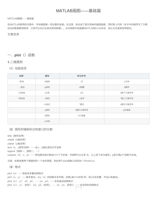
⽂章⽬录⼀、plot()函数1.⼆维图形(1)绘图选项线型颜⾊标记符号-实线b蓝⾊.点s⽅块:虚线g绿⾊o圆圈d菱形.-点划线r红⾊x叉v朝下三⾓符号-双划线c青⾊+加号^朝上三⾓符号m品红*星号<朝左三⾓符号y黄⾊>朝右三⾓符号p五⾓星k⿊⾊h六⾓星w⽩⾊(2)图形的辅助标注和窗⼝的分割title(图形说明)xlabel(x轴说明)ylabel(y轴说明)text(x,y图形说明)——在x,y轴处添加⽂字说明legend(图例⼀,图例⼆,…)subplot(m,n,p)——将绘图区域分割成m*n个⼦区域,并按照⾏从左⾄ 右,从上⾄下依次编号。
p表⽰第p个绘图⼦区域。
注意:如果是要两个图画到同⼀个坐标⾥⾯,则在两个plot函数之间添加⼀⾏hold on(3)格式plot(x)——缺省⾃变量绘图格式plot(x,y)——基本格式。
以y(x)的函数关系作图。
如果y是n*m的矩 阵,则x为⾃变量,作出m条曲线。
plot(x1,y1,x2,y2,…,xn,yn)——多条曲线绘图格式plot(x1,y1,选项1,x2,y2,选项2,…,xn,yn,选项n)——含选项的绘图格式x1=[1 2 3 4 5 6 7 8 9];x2=[2 4 6 8 10 12 14 16 18];y1=[1 4 9 16 25 36 49 64 81];y2=[18 16 14 12 10 8 6 4 2];subplot(4,1,1);plot(x1);title('例⼀');xlabel('⾃变量');ylabel('因变量');subplot(4,1,2);plot(x1,y1);title('例⼆');xlabel('⾃变量');ylabel('因变量');subplot(4,1,3);plot(x1,y1,x2,y2);title('例三');xlabel('⾃变量');ylabel('因变量');subplot(4,1,4);plot(x1,y1,'m+',x2,y2,'c*');title('例四');xlabel('⾃变量');ylabel('因变量');2.三维图形(1)格式plot3(x1,y1,z1,‘选项⼀’,x2,y2,z1,‘选项⼆’,…)x,y,z是长度相同的向量:⼀条曲线x,y,z是维度相同的矩阵:多条曲线(2)⽹格矩阵⽣成函数:meshgrid[X,Y]=meshgrid(x,y)x,y是给定的向量,X,Y是⽹格划分后得到的⽹格矩阵注意,这个函数⽤来⽣成⽹格矩阵,不是直接⽤来画图的,配合mesh使⽤。
MATLAB图形绘制技巧与实例
MATLAB图形绘制技巧与实例介绍:MATLAB是一种功能强大,广泛应用于科学计算和工程领域的软件平台。
它拥有丰富的图形绘制功能,可以用于可视化数据和传达研究成果。
本文将探讨一些MATLAB图形绘制的技巧和提供一些实例,让读者了解如何高效地利用MATLAB 绘制各种类型的图形。
一、基本绘图函数MATLAB中最基本的绘图函数是plot,它可以绘制二维图形。
可以通过指定x和y向量作为输入参数,将数据点连线绘制出来。
除了plot函数,还有其他一些常用的绘图函数,如scatter用于绘制散点图,bar用于绘制条形图,hist用于绘制直方图等。
这些函数具有丰富的参数选项,可以根据需要进行调整,以得到满意的图形效果。
二、自定义图形样式在MATLAB中,可以通过一些简单的命令实现图形样式的自定义。
例如,可以通过修改线型、颜色和点标记等属性,使得图形更加美观和易读。
除了利用内置的属性选项,还可以使用一些自定义的方法,如在plot函数中添加字符串参数来自定义线型和颜色。
三、多图绘制在某些情况下,需要在一个图形窗口中展示多个图形。
MATLAB提供了subplot函数,可以将图形窗口划分为多个小的绘图区域,并在每个区域中绘制不同的图形。
这对于比较不同数据集之间的关系或展示多个实验结果非常有用。
另外,还可以使用hold on和hold off命令,以在同一个图形窗口中绘制多个图形,并在绘制后保持图形的可编辑性。
四、3D图形绘制除了二维图形,MATLAB还支持绘制三维图形。
可以使用plot3函数将数据点绘制成三维曲线或散点图。
也可以使用mesh和surf函数绘制三维表面图,这在可视化函数和曲面的形状时非常有用。
通过调整视角和添加颜色映射等设置,可以使得3D图形更加生动和具有立体感。
五、图形标注和注释为了更好地传达和解释图形的含义,MATLAB提供了一些标注和注释功能。
可以使用xlabel、ylabel和title函数添加坐标轴标签和标题。
matlab图像处理基础实例
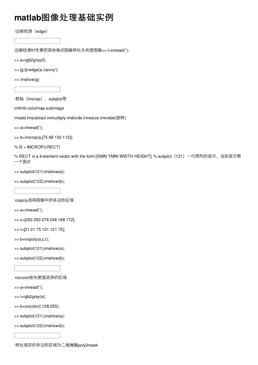
matlab图像处理基础实例·边缘检测(edge)边缘检测时先要把其他格式图像转化为灰度图像>> f=imread('');>> a=rgb2gray(f);>> [g,t]=edge(a,'canny');>> imshow(g)·剪贴(imcrop)、subplot等imfinfo colormap subimageimadd imsubtract immultiply imdivide imresize imrotate(旋转)>> a=imread('');>> b=imcrop(a,[75 68 130 112]);% I2 = IMCROP(I,RECT)% RECT is a 4-element vector with the form [XMIN YMIN WIDTH HEIGHT]; % subplot(121)⼀⾏两列的显⽰,当前显⽰第⼀个图⽚>> subplot(121);imshow(a);>> subplot(122);imshow(b);·roipoly选择图像中的多边形区域>> a=imread('');>> c=[200 250 278 248 199 172];>> r=[21 21 75 121 121 75];>> b=roipoly(a,c,r);>> subplot(121);imshow(a);>> subplot(122);imshow(b);·roicolor按灰度值选择的区域>> a=imread('');>> i=rgb2gray(a);>> b=roicolor(i,128,255);>> subplot(121);imshow(a);>> subplot(122);imshow(b);·转化指定的多边形区域为⼆值掩膜poly2mask>> x=[63 186 54 190 63];>> y=[60 60 209 204 60];>> b=poly2mask(x,y,256,256); >> imshow(b);>> holdCurrent plot held>> plot(x,y,'b','LineWidth',2)·roifilt2区域滤波a=imread('');i=rgb2gray(a);c=[200 250 278 248 199 172];r=[21 21 75 121 121 75];b=roipoly(i,c,r);h=fspecial('unsharp');j=roifilt2(h,i,b);subplot(121),imshow(i);subplot(122),imshow(j);·roifill区域填充>> a=imread('');>> i=rgb2gray(a);>> c=[200 250 278 248 199 172]; >> r=[21 21 75 121 121 75]; >> j=roifill(i,c,r); >> subplot(211);imshow(i);>> subplot(212);imshow(j);·FFT变换f=zeros(100,100);f(20:70,40:60)=1;imshow(f);F=fft2(f);F2=log(abs(F));imshow(F2),colorbar·补零操作和改变图像的显⽰象限f=zeros(100,100);f(20:70,40:60)=1;subplot(121);imshow(f);F=fft2(f,256,256);F2=fftshift(F);subplot(122);imshow(log(abs(F2)))·离散余弦变换(dct)>> a=imread('');>> i=rgb2gray(a);>> j=dct2(i);>> subplot(131);imshow(log(abs(j))),colorbar >> j(abs(j)<10)=0;>> k=idct2(j);>> subplot(132);imshow(i);>> subplot(133);imshow(k,[0,255]);info=imfinfo('')%显⽰图像信息·edge提取图像的边缘canny prewitt sobelradon函数⽤来计算指定⽅向上图像矩阵的投影>> a=imread('');>> i=rgb2gray(a);>> b=edge(i);>> theta=0:179;>> [r,xp]=radon(b,theta);>> figure,imagesc(theta,xp,r);colormap(hot); >> xlabel('\theta(degrees)'); >> ylabel('x\prime');>> title('r_{\theta}(x\prime)');>> colorbar·filter2均值滤波>> a=imread('');>> i=rgb2gray(a);>> imshow(i)>> k1=filter2(fspecial('average',3),i)/255;%3*3 >> k2=filter2(fspecial('average',5),i)/255;%5*5 >> k3=filter2(fspecial('average',7),i)/255;%7*7 >> figure,imshow(k1)>> figure,imshow(k2)>> figure,imshow(k3)wiener2滤波eg:k=wiener(I,[3,3]))medfilt2中值滤波同上deconvwnr维纳滤波马赫带效应(同等差⾊带条)·减采样>> a=imread('');>> b=rgb2gray(a);>> [wid,hei]=size(b);>> quarting=zeros(wid/2+1,hei/2+1); >> i1=1;j1=1;>> for i=1:2:widfor j=1:2:heiquarting(i1,j1)=b(i,j);j1=j1+1;endi1=i1+1;j1=1;end>> figure>> imshow(uint8(quarting))>> title('4倍减采样')>> quarting=zeros(wid/4+1,hei/4+1); i1=1;j1=1;for i=1:4:widfor j=1:4:heiquarting(i1,j1)=b(i,j);j1=j1+1;endi1=i1+1;j1=1;end>> figure,imshow(uint8(quarting)); title('16倍减采样')结论:在采⽤不同的减采样过程中,其图像的清晰度和尺⼨均发⽣了变化灰度级转化>> a=imread('');>> b=rgb2gray(a);>> figure;imshow(b)>> [wid,hei]=size(b);>> img2=zeros(wid,hei);>> for i=1:widfor j=1:heiimg2(i,j)=floor(b(i,j)/128);endend>> figure;imshow(uint8(img2),[0,2]) %2级灰度图像图像的基本运算>> i=imread('');>> figure;subplot(231);imshow(i);>> title('原图');>> j=imadjust(i,[.3;.6],[.1 .9]);%Adjust image intensity values or colormap图像灰度值或colormap调整% J = IMADJUST(I,[LOW_IN; HIGH_IN],[LOW_OUT; HIGH_OUT])>> subplot(232);imshow(j);title('线性扩展');>> i1=double(i);i2=i1/255;c=2;k=c*log(1+i2);>> subplot(233);imshow(k);>> title('⾮线性扩展');>> m=255-i;>> subplot(234);imshow(m)>> title('灰度倒置')>> n1=im2bw(i,.4);n2=im2bw(i,.7);>> subplot(235);imshow(n1);title('⼆值化阈值')>> subplot(236);imshow(n2);title('⼆值化阈值')图像的代数运算加。
matlab图像处理的几个实例
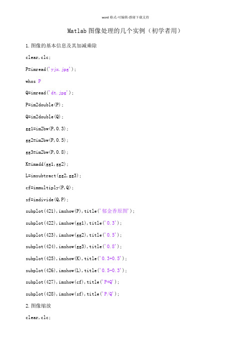
Matlab图像处理的几个实例(初学者用)1.图像的基本信息及其加减乘除clear,clc;P=imread('yjx.jpg');whos PQ=imread('dt.jpg');P=im2double(P);Q=im2double(Q);gg1=im2bw(P,0.3);gg2=im2bw(P,0.5);gg3=im2bw(P,0.8);K=imadd(gg1,gg2);L=imsubtract(gg2,gg3);cf=immultiply(P,Q);sf=imdivide(Q,P);subplot(421),imshow(P),title('郁金香原图');subplot(422),imshow(gg1),title('0.3');subplot(423),imshow(gg2),title('0.5');subplot(424),imshow(gg3),title('0.8');subplot(425),imshow(K),title('0.3+0.5');subplot(426),imshow(L),title('0.5-0.3');subplot(427),imshow(cf),title('P*Q');subplot(428),imshow(sf),title('P/Q');2.图像缩放clear,clc;I=imread('dt.jpg');A=imresize(I,0.1,'nearest');B=imresize(I,0.4,'bilinear');C=imresize(I,0.7,'bicubic');D=imresize(I,[100,200]);F=imresize(I,[400,100]);figuresubplot(321),imshow(I),title('原图');subplot(322),imshow(A),title('最邻近插值');subplot(323),imshow(B),title('双线性插值');subplot(324),imshow(C),title('二次立方插值');subplot(325),imshow(D),title('水平缩放与垂直缩放比例为2:1'); subplot(326),imshow(F),title('水平缩放与垂直缩放比例为1:4');灰度变换、直方图变换clear,clc;fg=imread('fg.jpg');zl=imread('zl.jpg');hfg=rgb2gray(fg);fg1=double(hfg);out1=255*(fg1/255).^0.7;out1(find(out1>255))=255;fg1=uint8(fg1);out1=uint8(out1);img=rgb2gray(zl);[harm,x]=imhist(img);J=histeq(hfg,harm);figuresubplot(421),imshow(fg1),title('复古灰度图');subplot(422),imhist(fg1),title('复古灰度图的直方图');subplot(423),imshow(out1),title('对复古灰度图像进行幂次变换'); subplot(424),imhist(out1),title('幂次变换图像的直方图');subplot(425),imshow(img),title('朱莉');subplot(426),imhist(img),title('朱莉图像对应的直方图');subplot(427),imshow(J),title('直方图变换后的复古图');subplot(428),imhist(J),title('直方图变换后的复古图对应的直方图');傅里叶变换、频域滤波1.傅里叶变换clear,clc;rgb=imread('zl.jpg');rgb=imresize(rgb,0.7,'bilinear');rgb=im2double(rgb);fR=rgb(:,:,1);fG=rgb(:,:,2);fB=rgb(:,:,3);flyfR=fft2(fR);flyfG=fft2(fG);flyfB=fft2(fB);Frgb(:,:,1)=flyfR;Frgb(:,:,2)=flyfG;Frgb(:,:,3)=flyfB;tzR=fftshift(flyfR);tzG=fftshift(flyfG);tzB=fftshift(flyfB);tzF(:,:,1)=tzR;tzF(:,:,2)=tzG;tzF(:,:,3)=tzB;iflyfR=ifft2(flyfR);iflyfG=ifft2(flyfG);iflyfB=ifft2(flyfB);out(:,:,1)=iflyfR;out(:,:,2)=iflyfG;out(:,:,3)=iflyfB;figuresubplot(221),imshow(rgb),title('原图');subplot(222),imshow(Frgb),title('图像频谱');subplot(223),imshow(tzF),title('调整中心后的图像频谱'); subplot(224),imshow(out),title('逆变换得到的原图');2.频域滤波clear,clc;I=rgb2gray(imread('ml.jpg'));J=imnoise(I,'gaussian',0.1);Jzz1=medfilt2(J,[3 3]);Jzz2=medfilt2(J,[10 10]);XJ=imnoise(I,'salt & pepper');f=im2double(XJ);g=fft2(f);g=fftshift(g);[M,N]=size(g);nn=2;d0=50;m=fix(M/2);n=fix(M/2);for i=1:Mfor j=1:Nd=sqrt((i-m)^2+(j-n)^2);h1=1/(1+0.414*(d/d0)^(2*nn));result1(i,j)=h1*g(i,j);endendresult1=ifftshift(result1);J2=ifft2(result1);J3=im2uint8(real(J2));figuresubplot(231),imshow(I),title('原图的灰度图像');subplot(232),imshow(J),title('加高斯噪声');subplot(233),imshow(Jzz1),title('模板3*3中值滤波后的图像'); subplot(234),imshow(Jzz2),title('模板10*10中值滤波后的图像'); subplot(235),imshow(J3),title('低通滤波图');彩色图像处理clear,clc;rgb=imread('yjx.jpg');fR=rgb(:,:,1);fG=rgb(:,:,2);fB=rgb(:,:,3);R=rgb;R(:,:,[2 3])=0;G=rgb;G(:,:,[1 3])=0;B=rgb;B(:,:,[1 2])=0;yiq=rgb2ntsc(rgb);fY=yiq(:,:,1);fI=yiq(:,:,2);fQ=yiq(:,:,3);fR=histeq(fR,256);fG=histeq(fG,256);fB=histeq(fB,256);RGB=cat(3,fR,fG,fB);figuresubplot(341),imshow(rgb),title('原图');subplot(342),imshow(R),title('图像的红色分量');subplot(343),imshow(G),title('图像的绿色分量');subplot(344),imshow(B),title('图像的蓝色分量');subplot(345),imshow(yiq),title('NTSC彩色空间');subplot(346),imshow(fY),title('亮度');subplot(347),imshow(fI),title('色调');subplot(348),imshow(fQ),title('饱和度');subplot(349),imshow(RGB),title('rgb均衡化后的彩色图像');原图最邻近插值双线性插值二次立方插值水平缩放与垂直缩放比例为2:1水平缩放与垂直缩放比例为1:4郁金香原图0.30.50.80.3+0.50.5-0.3P*Q P/Q原图图像的红色分量图像的绿色分量图像的蓝色分量NTSC 彩色空间亮度色调饱和度rgb 均衡化后的彩色图像原图图像频谱调整中心后的图像频谱逆变换得到的原图word 格式-可编辑-感谢下载支持原图的灰度图像加高斯噪声模板3*3中值滤波后的图像模板10*10中值滤波后的图像低通滤波图。
- 1、下载文档前请自行甄别文档内容的完整性,平台不提供额外的编辑、内容补充、找答案等附加服务。
- 2、"仅部分预览"的文档,不可在线预览部分如存在完整性等问题,可反馈申请退款(可完整预览的文档不适用该条件!)。
- 3、如文档侵犯您的权益,请联系客服反馈,我们会尽快为您处理(人工客服工作时间:9:00-18:30)。
实验三 MATLAB 的绘图一、实验目的:掌握利用MATLAB 画曲线和曲面。
二、实验内容:1、 在不同图形中绘制下面三个函数t ∈[0,4π]的图象,3个图形分别是figure(1),figure(2),figure(3)。
)sin(41.0321t e y ty t y t -===π说明:y 1 线型:红色实线,y 2 线型:黑色虚线,y 3: 线型:兰色点线分别进行坐标标注,分别向图形中添加标题‘函数1’,‘函数2’, ‘函数3’ 解答:源程序与图像: t=0:0.1:4*pi; y_1=t;y_2=sqrt(t);y_3=4*pi.*exp(-0.1*t).*sin(t); figure(1)plot(t,y_1,'-r'); title('函数1');xlabel('t');ylabel('y_1'); figure(2)plot(t,y_2,'--k'); title('函数2');xlabel('t');ylabel('y_2'); figure(3)plot(t,y_3,':b'); title('函数3');xlabel('t');ylabel('y_3');函数1ty 102468101214函数2t y 2函数3ty 32、 在同一坐标系下绘制下面三个函数在t ∈[0,4π]的图象。
(用2种方法来画图,其中之一使用hold on ) 使用text 在图形适当的位置标注“函数1”“函数2”,“函数3” 使用gtext 重复上面的标注,注意体会gtext 和text 之间的区别 解答: 方法一: 程序与图形: t=0:0.1:4*pi; y_1=t;y_2=sqrt(t);y_3=4*pi.*exp(-0.1*t).*sin(t); figure(1)plot(t,y_1,'-r'); gtext('函数1');xlabel('t');ylabel('y'); hold onplot(t,y_2,'--k'); gtext('函数2');hold onplot(t,y_3,':b'); gtext('函数3');2468101214-10-5051015ty方法二: t=0:0.1:4*pi; y_1=t;y_2=sqrt(t);y_3=4*pi.*exp(-0.1*t).*sin(t); figure(1)plot(t,y_1,'-r',t,y_2,'--k',t,y_3,':b'); xlabel('t');ylabel('y'); text(10,10,'函数1'); text(11,2,'函数2'); text(11,-5,'函数3');02468101214-10-5051015ty4、绘制ρ=sin(2θ)cos(2θ)的极坐标图源程序和图形: theta=0:pi/100:2*pi;rho=sin(2*theta).*cos(2*theta); polar(theta,rho);9027018005、绘制y=10x 2的对数坐标图并与直角线性坐标图进行比较。
在一个图形中绘制4个子图,分别使用plot 、semilogx 、semilogy 、loglog 函数进行绘制; 并且用title 进行标注;同时添加网格线 源程序与图像: x=0:0.1:5; y=10*x.^2;subplot(2,2,1) plot(x,x);title('plot 函数图');grid onsubplot(2,2,2) semilogx(x,y);title('semilogx 函数图');grid onsubplot(2,2,3) semilogy(x,y);title('semilogy');grid onsubplot(2,2,4) loglog(x,y);title('loglog 函数图');grid on0246246plot 函数图10-1101010100200300semilogx 函数图024610-210102104semilogy10-11010110-210102104loglog 函数图6、绘制下面函数在区间[-6,6]中的图象。
⎪⎩⎪⎨⎧>+-≤<≤=3,630,0,sin )(x x x x x x x y源程序和图像: x=-6:0.1:0; y_1=sin(x); plot(x,y_1,'-k');xlabel('x');ylabel('y'); gtext('y_1=sin(x)'); hold on x=0:0.1:3; y_2=x;plot(x,y_2,'--b'); gtext('y_2=x'); hold on x=3:0.1:6; y_3=-x+6; plot(x,y_3,':r'); gtext('y_3=-x+6');-6-4-20246-1-0.500.511.522.53xy7、三维空间曲线绘制t ∈[0,4π]x=cos(t); y=sin(t);使用plot3 和comet3分别绘制 源程序和图像:(彗星图用matlab 复制之后看不到,用的是截图) t=0:0.1:4*pi; x=cos(t); y=sin(t);subplot(2,1,1) plot3(t,x,y);subplot(2,1,2) comet3(t,x,y);8、分别用mesh 和surf 函数,绘制下面方程所表示的三维空间曲面,x 和y 的取值范围设为[-3,3]。
101022y x z +-=源程序和图像: x=-3:0.1:3; y=-3:0.1:3;[x,y]=meshgrid(x,y);z=(-(x.^2)/10)+((y.^2)/10);subplot(2,1,1) mesh(x,y,z); title('mesh plot');xlabel('x');ylabel('y');zlabel('z');subplot(2,1,2) surf(x,y,z); title('surf plot');xlabel('x');ylabel('y');zlabel('z');4xmesh plotyz4xsurf plotyz9、用mesh 和surf 函数来绘制激光器输出横模的三维分布对于激光腔长为L=10, 激光波长λ=1064nm 方形镜共焦腔,其输出的几个横模如下所示意 其中πλωL os =00模的振幅分布()πλ/0022,L y x ey x v +-=10模的振幅分布()222,10osy x xey x v ω+-=01模的振幅分布()222,01osy x yey x v ω+-=20模的振幅分布()222)4(,2220osyxosexyxvωω+--=11模的振幅分布()222,11osyxxyeyxvω+-=%激光器输出横模的三维分布L=10e-2; %腔长Lambda=1064e-9;%波长w_os=sqrt(L*Lambda/pi);x=[-10:0.1:10];y=[-10:0.1:10];[x,y]=meshgrid(x,y);v_00=exp(-(x^2+y^2)/w_os^2);v_10=x*exp(-(x^2+y^2)/w_os^2);v_01=y*exp(-(x^2+y^2)/w_os^2);v_20=(4*x^2-w_os^2)*exp(-(x^2+y^2)/w_os^2); v_11=x*y*exp(-(x^2+y^2)/w_os^2);%00模figure(1)subplot(1,2,1)mesh(x,y,v_00);title('00模mesh图');subplot(1,2,2)surf(x,y,v_00);title('00模surf图');%10模figure(2)subplot(1,2,1)mesh(x,y,v_10);title('10模mesh图');subplot(1,2,2)surf(x,y,v_10);title('10模surf图');%01模figure(3)subplot(1,2,1)mesh(x,y,v_01);title('01模mesh图');subplot(1,2,2)surf(x,y,v_01);title('01模surf图');%20模 figure(4)subplot(1,2,1) mesh(x,y,v_20);title('20模mesh 图'); subplot(1,2,2) surf(x,y,v_20);title('20模surf 图');%11模 figure(5)subplot(1,2,1) mesh(x,y,v_11);title('11模mesh 图'); subplot(1,2,2) surf(x,y,v_11);title('11模surf 图');-0.010.0100模mesh 图-0.0100模surf 图-0.010.01x 10-410模mesh 图-0.010.010.01x 10-410模surf 图0.01-0.01-8-6-4-202468-401模mesh 图-0.010.01-401模surf 图-0.010.01x 10-620模mesh 图-0.010.01x 10-620模surf图-0.010.01x 10-711模mesh图-0.010.01x 10-711模surf 图10、分别绘制隐函数曲线1)x 2+y 2=1 程序与图像: x=-1:0.1:1; y=-1:0.1:1;ezplot('x.^2+y.^2-1'); title('x^2+y^2=1');xyx 2+y 2=1-6-4-202462)X 3+y 3=5xy 程序与图像: x=-10:0.1:10; y=-10:0.1:10;ezplot('x.^3+y.^3-5*x.*y'); title('x^3+y^3=5*x*y');xyx 3+y 3=5*x*y-6-4-2024611,在光纤放大器的文献中,我们经常能碰到双Y 轴图形的绘制,在某次实验中有人得到如下的实验数据,请绘制双Y 轴图形,横坐标为输入信号功率,纵坐标分别为输出功率和增益 输入的信号光功率(mW):1;2;3;4;5;6;7;8;9;10输出的信号光功率(mW):1.1;4.2;9.2;16.1;25.3;36.0;49.4;64.5;82.0;99.9标注横坐标为Input signal power (mW),纵坐标分别为Output power (mW); Gain(dB) 解答:程序与图像:Input=[1 2 3 4 5 6 7 8 9 10];Output=[1.1 4.2 9.2 16.1 25.3 36.0 49.4 64.5 82.0 99.9]; G=Output./Input; Gain=10log10(G);[AX,H1,H2]=plotyy(Input,Output,Input,Gain);set(get(AX(1),'Ylabel'),'String','Output power (mW)') set(get(AX(2),'Ylabel'),'String','Gain(dB)') xlabel('Input signal power (mW)');41020406080100O u t p u t p o w e r (m W )Input signal power (mW)12356789G a i n (d B )12,饼图的绘制我校某级光信专业本科生源分别为:湖北40人,安徽3人,黑龙江4人,贵州2人,江西5人,请绘制饼图和进行标注为湖北,安徽,黑龙江,贵州,江西;另外在饼图中把安徽,黑龙江学生的部分分离出来, 程序和图像: x=[40 3 4 2 5]; y=[0 1 1 0 0];pie(x,y,{'湖北40人','安徽3人', '黑龙江4人', '贵州2人','江西5人'}) title('我校某级光信专业本科生源');徽3人4人江西5人我校某级光信专业本科生源。