动态分析(DynamicAnalyzer)基础理论
动态分析方法
动态分析的方法一、单井动态分析单井动态分析包括油井动态分析和注水井动态分析,以研究阶段性的分层调整管理措施为主。
油田的变化总要通过单井反映出来,所以管好油、水井是管好油田的基点。
油井分析以所管某一油井为重点联系到周围有关的注水井和相邻油井进行综合分析。
注水井分析则以所管某一注水井为中心,联系到周围的油、水井进行综合分析。
现分述如下。
(一)油井动态分析对注水开发的油田来说,油井动态分析的目的就是要在保证达到一定采油速度的前提下实现三稳迟见水。
三稳就是产量稳、地层压力稳、流动压力稳。
迟见水就是无水采油期长、无水采收率高。
油井动态分析方法可综合为以下几点:第一,清点油层。
对所管油井的各小层要进行清点,了解全井射开的油层数、有效厚度和产能系数;了解射开各单层的类型,如水驱层(与注水井连通)、弹性层(与注水井不连通,与其它油井连通)、“土豆”层(与邻井全不连通)和“危险”层(与注水连通特别好,有见水危险);了解每个单层的渗透性、厚度和储量,掌握油层特性,胸中有数,分析就主动了。
第二,核实资料。
油井的生产特点和变化规律,总要通过观察现象和整理资料才能掌握。
在平时就必须取准油井动态资料,如油管压力、套管压力、流动压力、地层压力、产油量、油气比和油样分析资料(含水、含蜡、含砂等)。
及时观察记录油井变化情况如结蜡软硬、原油乳化、出砂、油井间歇出液现象。
新的变化情况出现后,要先从地面查清原因,弄清情况,落实资料,然后再进行动态分析。
第三,联系历史。
油井的每一变化都是有其根源的,要结合油井开采历史进行分析。
一方面要熟悉井史,结合钻井、固井、诱喷等有关情况进行分析。
另一方面要应用采油曲线,研究每个开采时期的生产指标变化特点,由它的过去,分析它的现在,由它的现在预测它的将来。
分析哪些是一贯的规律,哪些是突然的变化,便于综合考虑,得出系统概念。
第四,对比邻井。
首先要和注水井对比,如果见到注水效果或者见水,就要顺着连通层追踪到注水井,综合分析。
DynamicSignalAnalyzer:动态信号分析仪
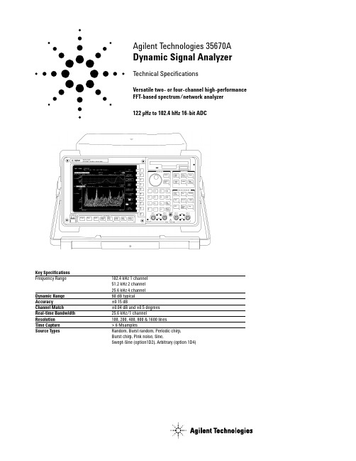
Agilent Technologies 35670A Dynamic Signal Analyzer Technical SpecificationsVersatile two- or four-channel high-performance FFT-based spectrum/network analyzer122 µHz to 102.4 hHz 16-bit ADCSignal Averaging (FFT Mode)Average Types (1 to 9,999,999 averages)RMS TimeExponentialRMS Exponential Peak HoldTimeAveraging ControlsOverload RejectFast Averaging On/OffUpdate Rate SelectSelect Overlap Process PercentagePreview Time RecordMeasurement ControlStart MeasurementPause/Continue MeasurementTriggeringContinuous (Freerun)External (Analog or TTL Level)Internal Trigger from any ChannelSource Synchronized TriggerGPIB TriggerArmed TriggersAutomatic/ManualRPM StepTime StepPre- and Post-Trigger Measurement DelayTachometer Input:±4V or ±20V range40 mv or 200 mV resolutionUp to 2048 pulses/revTach hold-off controlSource OutputsRand om BurstRand omPeriodic Chirp Burst ChirpPink Noise Fixed SineNote: Some source types are not available foruse in optional modes. See option description fordetails.Input ChannelsManual Range Anti-alias Filters On/OffUp-Only Auto Range AC or DC CouplingUp/Down Auto Range LED Half Range andOverload IndicatorsFloating or Grounded A-Weight Filters On/OffT ransducer power supplies (4 ma constant current)Frequency20 Spans from 195 mHz to 102.4 kHz (1 channel mode)20 Spans from 98 mHz to 51.2 kHz (2 channel mode)Digital zoom with 244 µHz resolution throughoutthe 102.4 kHz frequency bands.Resolution100, 200, 400, 800 and 1600 linesWindowsHann UniformFlat Top Force/ExponentialMath+,-,*, / ConjugateMagnitude Real and ImaginarySquare Root FFT, FFT-1LN EXP*jωor /jω PSDDifferentiation A, B, and C weightingIntegration Constants K1 thru K5Functions F1 thru F5AnalysisLimit Test with Pass/FailData Table with Tabular ReadoutData EditingTime Capture FunctionsCapture transient events for repeated analysis in FFT, octave, order, histogram, or correlation modes (except swept-sine). Time-captured data may be saved to internal or external disk, or transferred over GPIB. Zoom on captured data for detailed narrowband analysis. Up to6 Msamples of data can be saved inthe standard unit.Data Storage FunctionsBuilt-in 3.5 in., 1.44-Mbyte flexible disk also supports 720-KByte disks, and 2 Mbyte NVRAM disk. Both MS-DOS® and HP-LIF formats are available. Data can be formatted as either ASCII or Binary (SDF). The 35670A provides storage and recall from the internal disk, internal RAM disk, internal NVRAM disk, or external GPIB disk for any of the following information: Instrument Setup States Trace DataUser-Math LimitDataTime Capture Buffers Agilent Instrument BASIC Waterfall Display Data ProgramsData Tables Curve Fit/Synthesis TablesInterfacesGPIB (IEEE-488.1 and 488.2)ParallelRS-232C SerialHard-Copy OutputTo Serial or Parallel HP-GL Plotters (PCL5e)To Raster PrintersTo Serial or Parallel HP-GL PrintersTo Disk File (Supports Raster Printer,HP-GL Plotter, and HP-GL Printer)Time StampGPIB CapabilitiesListener/Talker (Direct control of plotters, printers, disk drives)Conforms to IEEE 488.1/488.2Conforms to SCPI 1992Controller with Agilent Instrument Basic option Standard Data Format (SDF) Utilities Exchange data between virtually all Agilent Dynamic Signal AnalyzersEasy data transfer to spreadsheetsData transfer to MATRIX X and MatlabSDF utilities run in an external PCCalibration & MemorySingle or Automatic CalibrationBuilt-In Diagnostics & Service Tests Nonvolatile Clock with Time/DateTime/Date Stamp on Plots and Saved Data Files Online HelpAccess to Topics via Keyboard or IndexFanOn/OffMS-DOS®is a U.S. registered trademark ofMicrosoft Corporation.Summary of Featureson Standard InstrumentThe following features are standardwith the Agilent 35670A:Instrument ModesFFT Analysis Histogram/Time Correlation Analysis Time Capture MeasurementFrequency DomainFrequency Response Power SpectrumLinear Spectrum CoherenceCross Spectrum Power SpectralDensityTime Domain (oscilloscope mode)Time Waveform AutocorrelationCross-Correlation OrbitDiagram Amplitude DomainHistogram, PDF, CDFTrace CoordinatesLinear Magnitude Unwrapped PhaseLog Magnitude Real PartdB Magnitude Imaginary PartGroup Delay Nyquist DiagramPhase PolarTrace UnitsY-axis Amplitude: combinations of units, unit value, calculated value, and unit format describey-axis amplitudeUnits: volts, g, meters/sec2, inches/sec2,meters/sec, inches/sec, meters, mils, inches, pascals, Kg, N, dyn, lb, user-defined EUsUnit Value: rms, peak, peak-to-peakCalculated Value: V, V2, V2/Hz, √Hz, V2s/Hz (ESD)Unit Format: linear, dB’s with user selectable dB reference, dBm with user selectable impedance.Y-Axis Phase:degrees, radiansX-Axis:Hz, cpm, order, seconds, user-definedDisplay FormatsSingleQuadDual Upper/Lower TracesSmall Upper and Large LowerFront/Back Overlay TracesMeasurement StateBode DiagramWaterfall Display with Skew, -45 to 45 DegreesTrace Grids On/OffDisplay BlankingScreen SaverDisplay ScalingAutoscale SelectableReference Manual Scale Linear or Log X-Axis Input Range Tracking Y-Axis LogX & Y Scale Markers with Expand and Scroll Marker FunctionsIndividual Trace MarkersCoupled Multi-Trace MarkersAbsolute or Relative MarkerPeak SearchHarmonic MarkersBand MarkerSideband Power MarkersWaterfall MarkersTime Parameter MarkersFrequency Response Markers23Agilent 35670A Specifications* Option AY6 single channel maximum range extends to 102.4 kHz without anti-alias filter protection.** Show All Lines mode allows display of up to 131.1,65.5 and 32.7 kHz respectively. Amplitudes accuracy is unspecified and not alias protected.<-80 dBfs<-80 dBfs0 dBfs, ≤1 MHz 200 kHz with IEPE transducer power supply On)800 Hz Span-51 -41 -31 -21 -11 270.0028 0.0089 0.028 0.089 0.28022.4Amplitude Range (dBVrms / Vrms)51.2 kHz Span 6.4 kHz Span 456Computed Order Tracking - Option 1D0()Maximum Order x Maximum RPM≤60Online (Real Time) 1 Channel Mode 25,600 Hz2 Channel Mode 12,800 Hz4 Channel Mode 6,400 HzCapture Playback 1 Channel Mode 102,400 Hz2 Channel Mode 51,200 Hz4 Channel Mode 25,600 HzNumber of Orders ≤200 5 ≤RPM ≤491,519(Maximum useable RPM is limited byResolution, Tach Pulse Rate,Pulses/Revolutionand Average Mode Settings.)Delta Order1/128 to 1/1Resolution ≤400(Maximum Order) / (Delta Order)Maximum RPM Ramp Rate1000 RPM / second real-time (typical)1000 - 10,000 RPM Run UpMaximum Order 10Delta Order 0.1RPM Step 30 (1 Channel)60 (2 Channel)120 (4 Channel)Order T rack Amplitude Accuracy±1 dB (typical)Real Time Octave Analysis - Option 1D1Standards Conforms to ANSI Standard S1.11 - 1986,Order 3, Type 1-D, Extended and OptionalFrequency RangesConforms to IEC 651-1979 Type 0 Impulse ,and ANSI S1.4Frequency Ranges(at centers)Online (Real Time):Single Channel 2 Channel 4 Channel1/1 Octave 0.063 - 16 kHz 0.063 - 8 kHz 0.063 - 4 kHz1/3 Octave 0.08 - 40 kHz 0.08 - 20 kHz 0.08 - 10 kHz1/12 Octave 0.0997 - 12.338 kHz0.0997 - 6.169 kHz 0.0997 - 3.084 kHzCapture Playback:1/1 Octave 0.063 - 16 kHz 0.063 - 16 kHz 0.063 - 16 kHz1/3 Octave 0.08 - 31.5 kHz 0.08 - 31.5 kHz 0.08 - 31.5 kHz1/12 Octave 0.0997 - 49.35 kHz 0.0997 - 49.35 kHz 0.0997 - 49.35 kHzOne to 12 octaves can be measured and displayed.1/1-, 1/3-, and 1/12-octave true center frequencies related by the formula: f(i+1)/f(i) = 2^(1/n); n=1,3, or 12; Where 1000 Hz is the reference for 1/1, 1/3 Octave, and 1000*2^(1/24) Hz is the referencefor 1/12 octave. The marker returns the ANSI standard preferred frequencies.Accuracy1 Second Stable AverageSingle Tone at Band Center: ≤±0.20 dBReadings are taken from the Linear Total Power Spectrum Bin.It is derived from sum of each filter.1/3-Octave Dynamic Range > 80 dB (typical) per ANSI S1.11-19862 Second Stable AverageTotal power limited by input noise level7General SpecificationsSafety Standards CSA Certified for Electronic Test andMeasurement Equipment per CSAC22.2, NO. 231This product is designed for compliance to:UL1244, Fourth EditionIEC 348, 2nd Edition, 1978EMI / RFI Standards CISPR 11Acoustic Power LpA < 55 dB (Cooling Fan at High Speed Setting)< 45 dB (Auto Speed Setting at 25 °C)Fan Speed Settings of High, Automatic, and Off are available. The Fan Off setting can be enabledfor a short period of time, except at higher ambient temperatures where the fan will stay on. Environmental Operating RestrictionsOperating: Operating: Storage&Disk In Drive No Disk In Drive TransportAmbient Temp. 4 °C to 45 °C 0 °C to 55 °C -40 °C to 70 °C Relative Humidity(non-condensing)Minimum 20% 15% 5%Maximum 80% at 32 °C 95% at 40 °C 95% at 50 °C Vibrations 0.6 Grms 1.5 Grms 3.41 Grms(5 - 500 Hz)Shock 5G(10 mSec 1/2 sine) 5G (10 mSec 1/2 sine) 40G (3 mSec 1/2 sine) Max. Altitude 4600 meters 4600 meters 4600 meters(15,000 ft.) (15,000 ft.) (15,000 ft.)AC Power90 Vrms - 264 Vrms(47 - 440 Hz)350 VA maximumDC Power12 VDC to 28 VDC Nominal200 VA maximumDC Current at 12V standard: <10A typical4 channel: <12A typicalWarm-Up Time 15 minutesWeight 15 kg (33 lb) net29 kg (64 lb) shippingDimensions(Excluding Bail Handle and Impact Cover) Height 190 mm (7.5")Width 340 mm (13.4")Depth 465 mm (18.3")AbbreviationsdBVrms = dB relative to 1 Volt rms.dBfs = dB relative to full scale amplituderange. Full scale is approx. 2 dB below ADCoverload.Typical = typical, non-warranted, performancespecification included to provide generalproduct information.By internet, phone, or fax, get assistance with all your test & measurement needsOnline assistance:/find/assistPhone or FaxUnited States:(tel) 800 452 4844Canada:(tel) 877 894 4414(fax) 905 282 6495China:(tel) 800 810 0189(fax) 800 820 2816Europe:(tel) (31 20) 547 2323(fax) (31 20) 547 2390Japan:(tel) (81) 426 56 7832(fax) (81) 426 56 7840Korea:(tel) (82 2) 2004 5004(fax) (82 2) 2004 5115Latin America:(tel) (305) 269 7500(fax) (305) 269 7599Taiwan:(tel) 0800 047 866(fax) 0800 286 331Other Asia Pacific Countries:(tel) (65) 6375 8100(fax) (65) 6836 0252Email:*******************Product specifications and descriptions in this document subject to change without notice.© Agilent Technologies, Inc. 2003Printed in USA March 21, 20035966-3064E/find/emailupdatesGet the latest information on theproducts and applications you select.Agilent T&M Software and ConnectivityAgilent's Test and Measurement softwareand connectivity products, solutions anddeveloper network allows you to take timeout of connecting your instruments to yourcomputer with tools based on PCstandards, so you can focus on your tasks,not on your connections. Visit/find/connectivityfor more information.Test Equipment Connection Corporation is your single source test & measurement solution. We offer over 400 test equipment manufacturers including Agilent, Tektronix, Anritsu, Rohde & Schwarz, Advantest, Megger, LeCroy, Chroma and Fluke, plus thousands of New, Used, Second Hand, Pre-Owned, Demo, Refurbished, and Reconditioned test equipment products.For over 18 years, we have been providing high quality spectrum analyzers, mobile phone testers, oscilloscopes, network analyzers, service monitors, RF amplifiers, broadband amplifiers, signal generators, OTDR, fusion splicers, and digital multimeters at great savings to over 200,000 customers worldwide. Lease or rent from us, and we can help manage your idle assets using our consignment program. Trade in underutilized test equipment for cash or credit towards the test solutions you need today! TEC offers repair and calibration support for thousands of current and discontinued brands. TEC's GSA Contract #GS-07F-0358U provides lower cost test and measurement equipment to qualifying government contractors and agencies.Click Here to Request an Offer on Your Surplus Test and Measurement Assets Today。
动态分析
动态频率响应分析示例
位移与频率的关系(无阻尼情况) 由上图可知,稳定的周期性载荷,在频率与工作台低阶固有频率(特别是第一阶)接 近时导致变形急剧增大,这样说明设计产品时外界载荷应避免与产品低阶固有频率一 致而导致共振发生危险。
动态频率响应分析示例
上图频率范围过大,对于载荷的实际工作频率测量不够密集,再运行一次动态频率响 应分析,获取频率更低的数据,如下图所示为0---160Hz的数据。
前10阶固有频率
最大Von Mises 应力与时间的关系
动态时间响应分析示例
Von Mises应力
位移
速度
加速度
应变
各种云图结果
应变能
动态时间响应分析示例
范例示意图
对称拉伸100
动态时间响应分析示例
两个测量点阻尼为3%的动态时域图表结果
动态时间响应分析示例
两个测量点阻尼为50%的动态时域图表结果
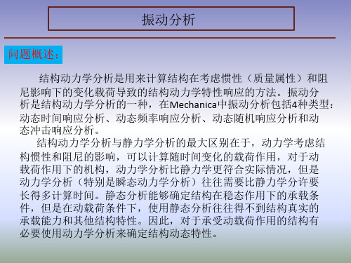
振动分析
问题概述:
结构动力学分析是用来计算结构在考虑惯性(质量属性)和阻 尼影响下的变化载荷导致的结构动力学特性响应的方法。振动分 析是结构动力学分析的一种,在Mechanica中振动分析包括4种类型: 动态时间响应分析、动态频率响应分析、动态随机响应分析和动 态冲击响应分析。 结构动力学分析与静力学分析的最大区别在于,动力学考虑结 构惯性和阻尼的影响,可以计算随时间变化的载荷作用,对于动 载荷作用下的机构,动力学分析比静力学更符合实际情况,但是 动力学分析(特别是瞬态动力学分析)往往需要比静力学分许要 长得多计算时间。静态分析能够确定结构在稳态作用下的承载条 件,但是在动载荷条件下,使用静态分析往往得不到结构真实的 承载能力和其他结构特性。因此,对于承受动载荷作用的结构有 必要使用动力学分析来确定结构动态特性。
关于有限元动态分析的一些关键概念

2021/3/7
4
2 模态叠加
是用于瞬态分析和谐分析的一种求解技术模态叠加是将从模态分析中得到各个振型分别乘以系 数后叠加起来以计算动力学响应。它是一个用来求解线性动力学问题的快速、有效的方法。另一种 可选用的方法是直接积分方法,这种方法需要较多的时间。
模态数指一个结构拥有模态的个数。
对一般形状的振型,它可以看成是很多不同阶的形状的组合。阶数与振型相对应。有多少个振 型就有多少个阶数。对应基本周期的振型称为第一阶振型,比第一周期略小的(第二周期)对应的振 型称为第二阶……第n阶,依次类推。从理论上来说,任何结构的固有频率都有无限多个,按频率大 小排列,数值最小的为一阶频率。但在用有限元进行计算时只能求出有限多个固有频率(与无约束 的自由度个数相同),且阶数越高,误差越大。但对实际结构有意义的恰是频率较小的若干阶频率。 然而,为了便于对模态进行称呼,就以模态频率的大小进行排队,这种排队的顺序往往就是所谓的 “阶”,一个系统有几阶模态,理论上是N个自由度系统存在N个模态,而低阶模态的模态刚度相 对比较弱,在同样量级的激励作用下,响应会相对所占的权值大一些,所以,工程上低阶模态比较 被受关照,理论上低阶模态理论也相对成熟。
2021/3/7
2
一个物体有很多个固有振动频率(理论上无穷多个),按照从小到大顺序,第一个就叫第一阶 固有频率,依次类推。所以模态的阶数就是对应的固有频率的阶数。
振型是指体系的一种固有的特性。它与固有频率相对应,即为对应固有频率体系自身振动的 形态。每一阶固有频率都对应一种振型。振型与体系实际的振动形态不一定相同。振型对应于 频率而言,一个固有频率对应于一个振型。按照频率从低到高的排列,来说第一振型,第二振 型等等。此处的振型就是指在该固有频率下结构的振动形态,频率越高则振动周期越小。在实 验中,我们就是通过用一定的频率对结构进行激振,观测相应点的位移状况,当观测点的位移 达到最大时,此时频率即为固有频率。实际结构的振动形态并不是一个规则的形状,而是各阶 振型相叠加的结果。
动态分析方法
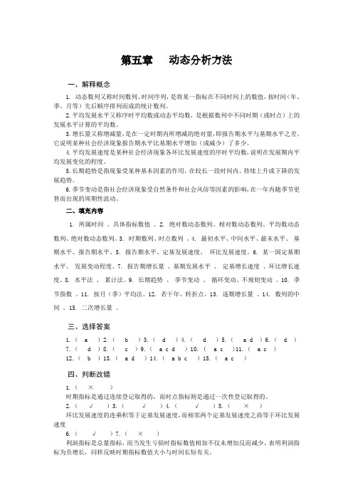
第五章动态分析方法一、解释概念1. 动态数列又称时间数列、时间序列,是将某一指标在不同时间上的数值,按时间(年、季、月等)先后顺序排列而成的统计数列。
2.平均发展水平又称序时平均数或动态平均数,是根据数列中不同时期(或时点)上的发展水平计算的平均数。
3.增长量又称增减量,是在一定时期内所增减的绝对量,即报告期水平与基期水平之差。
它说明某种社会经济现象报告期水平比基期水平增加(或减少)了多少。
4.平均发展速度是某种社会经济现象各环比发展速度的序时平均数,说明在发展期内平均发展变化的程度。
5.长期趋势是指现象受某种基本因素的作用,在较长一段时间内,持续上升或下降的发展趋势。
6.季节变动是指社会经济现象受自然条件和社会风俗等因素的影响,在一年内随季节更替而出现的周期性波动。
二、填充内容1. 所属时间、具体指标数值。
2.绝对数动态数列、相对数动态数列、平均数动态数列、绝对数动态数列。
3. 时期数列、时点数列。
4. 最初水平、中间水平、最末水平、基期水平、报告期水平。
5. 报告期水平、定基发展速度、环比发展速度。
6. 某一固定基期水平、发展变动程度。
7. 报告期增长量、基期发展水平、定基增长速度、环比增长速度。
8. 水平法、累计法。
9. 长期趋势、季节变动、循环变动、不规则变动。
10. 季节指数。
11. 按月(季)平均法。
12. 若干年、转折点。
13. 逐期增长量。
14. 数列的中间。
15. 二次增长量。
三、选择答案1.( a )2.( b )3.( d )4.( d )5.( a d )6.( d )7.( d )8.( c )9.( a c d )10. ( a c )11.( a c )12.( b )13.( a d )14.( a b c )15.( a c )四、判断改错1.(×)时期指标是通过连续登记取得的,而时点指标则是通过一次性登记取得的。
2.(√)3.(√)4.(√)5.(×)环比发展速度的连乘积等于定基发展速度,而相邻两个定基发展速度之商等于环比发展速度6.(√)7.(×)利润指标是总量指标,而当发生亏损时指标数值相加不仅未增加反而减少,表明利润指标为负增长,同样反映时期指标数值大小与时间长短有关。
动态分析

或气体影响。 左下角:分析光杆在下死点时出现的问题,如固定阀的漏失等情况。
二、油井常见故障诊断
几种典型的示功图分析
1、气体对示功图的影响 2、漏失对示功图的影响 3、活塞被卡在泵筒中不能动的示功图 4、连喷带抽的示功图 5、抽油杆柱断或脱扣的示功图 6、油井出砂的示功图 7、油井结蜡示功图 8、上冲程活塞脱出泵筒示功图 9、下死点处活塞碰固定阀的示功图 10、上冲程光杆接箍挂井口示功图 11、油管漏的示功图
理论示功图
B B1 C
KN
高 压 区
上行
油 套 环 空
低 压 区
A
P1
D P
低 压 区
下行
油 套 环 空
C:上死点; A:下死点; CD:卸载线 D:排出点 AB:加载线; B:吸入点 BB1:油管和油杆弹性形变,冲程损失;
s
高 压 区
P:油杆在液中的重量 P1:活塞上液柱重量
二、油井常见故障诊断
0 500 1000 1500 2000 2500
2004年10月 2005年1月 2005年4月 2005年7月 2005年10月 2006年1月
实测示功图分析 KN
5 4 3 2 1 0
W3-5井采油曲线
日产液量 日产油量 含水
16 14 12 10 8 6 4 2 0
1月1日 1月8日 1月15日 1月22日 1月29日 2月5日 2月12日 2月19日 2月26日 3月5日
2
由于泵漏,使油井产量下降或达不到正常产量。
3
当动液面或产量突然发生变化时,为了查明原 因,采取恰当措施,需要进行探砂面与冲砂等。
4
抽油泵工作失灵,游动阀或固定阀被砂、蜡或 其他赃物卡住。
5.动态分析1
5.1动态分析概述一、动态分析概述动态分析是指这样一种分析类型:其目的是探寻和研究变量的具体时间路径,或者是确定在给定的充分长的时间内,这些变量是否会趋向收敛于某一(均衡)值。
这方面的研究是非常重要的,因为它可以弥补静态学和比较静态学的严重不足。
在比较静态学中,我们总是武断地假设:经济调节过程不可避免地导致均衡。
而在动态分析中,我们直接面对均衡的“可实现性”问题,而不是假设它必然能够实现。
动态分析的一个显著特征是确定变量的时间,这就把时间因索明确纳入分析范围。
有两种方式可以做到这一点:我们可以将时间视为连续变量,也可将其视为离散变量。
前者变量在每一时点都要发生某些变化(如在连续计算复利时那样),在后一种情况下,变量仅在某一时段内才发生某些变化(如仅每六个月末才记入利息)。
前一种情况可以借助微分方程来求解;后一种情况可以借助于差分方程来求解。
一般面言,静态模型中的问题是要求出满足某些特定均衡条件的内生变量的值。
把静态学应用于最优化模型时,任务变成求使目标函数最大比(或最小化)的选择变量的值——而一阶条件充当均衡条件。
与此相对照的是,动态模型涉及的问题是,在已知变化模式的基础上(比如,给定瞬时变化率),描述某些变量的变化时间路径。
举个例子或许会使问题更清楚。
例1:假定己知人口规模H 随时间以速率t dtdH 1-=变化。
则我们要求的是:人口H=H (t )的何种时间路径可以产生上述变化率。
通过积分可解得该速率函数的原函数c t H t+=212)(。
为了确定函数中常数c 的具体值,我们还需要初始条件或边界条件。
假设初始人口H (0)=100,令所求原函数中t=0,代入可得H (0)=c=100。
所以在这一初始条件下1002)(1+=tt H 。
更一般地,对于任意给定初始人口H (0)时间路径将为)0(2)(21H t H t+=课下复习不定积分、定积分和广义积分和微分方程的相关内容,特别注意其基本法则。
MS-基本原理与仪器结构(2)
2019/7/5
12
质谱分析法-基本原理及仪器结构
2019/7/5
13
质谱分析法-基本原理及仪器结构
例:要鉴别N+2(m/z为28.006)和CO+(m/z为 27.995)两个峰,仪器的分辨率至少是多少? 在某质谱 仪上测得一质谱峰中心位置为245u,峰高5%处的峰宽为
0.52u,可否满足上述要求?
线射入质量分析器。离子加速电压值因质量分析
器不同而不同。
离子化的方法下面进一步介绍。
2019/7/5
28
质谱分析法-基本原理及仪器结构
离子化的方法
电子轰击电离 Electron Impact Ionization, EI
化学离子化 Chemical Ionization, CI
场电离,场解吸 Field Ionization FD, Field Desorption FD 快原子轰击 Fast Atom Bombardment, FAB
质谱计框图
进样系统
真空系统
加速区
2019/7/5
计算机数据 处理系统
离子源 质量分析器
产生气相离子
按离子的质量与 电荷比分离离子
检测器
离子转换成电信号
6
质谱分析法-基本原理及仪器结构
1、进样 化合物通过汽化引入离子化室;
2、离子化
在离子化室,组分分子被一束加速电子碰 撞(能量约70eV),撞击使分子电离形 成正离子;
5、加速离子进入一个强度为H的磁场,发
生偏转,半径为:
r mv
(2)
zH
将(1)(2)合并:
m H 2r2
(3)
Z 2V
当 r 为仪器设置不变时,改变加速电压或磁
DMA资料解析
各向异性材料
➢ “各向异性材料在不同的方向上具有不同的特性。 例如,纤维,木材,取向的无定型高分子,注塑 的样品,纤维填充的复合材料,单晶,结晶性有 序排列的结晶高分子。所以各向异性的材料比各 向同性的材料更常见。”
➢ 具有两个以上独立的模数-通常最少5或6个。 ➢ 独立模数的个数取决于材料的对称性。
➢ 非常刚硬的固体 ➢ 从硬到软的橡胶 ➢ 粘弹性流体
➢ 高分子的力学强度是以下因素的结果:
➢ 高分子的化学组成 ➢ 决定力学性能在何处发生变化
➢ 高分子的物理分子结构 ➢ 决定力学性能如何发生变化
典型无定型高分子材料的粘弹谱
Glassy Region
Transition Region
Rubbery Plateasile or compressive stress(单轴拉伸或压缩应力)
t = shear stress(剪切应力)
shyd = hydrostatic tensile or compressive stress(静态拉伸或压缩应力) e = normal strain(正向应变)
➢ s = tensile stress, t = shear stress
➢应变 = 几何形状的改变 [无量纲]
➢ e = tensile strain, g = shear strain
➢应变或剪切速率 = 速率梯度: d(strain)/dt [1/s]
➢ e = tensile strain rate, g = shear strain rate
固体高分子流变学的重要性
➢ 高分子材料被广泛的应用
➢ 宽泛的力学特性 ➢ 成本上经济
➢ 对大多数的应用,在高分子所有的物理化学特性中, 力学特性被认为是最重要的。
DynamicMechanicalAnalyzer動態黏彈性機械分析儀
DMA Measuring System Installation
16
DMA Measuring Systems
17
DMA 3-Point Bending Measuring System
*不鏽鋼/石英 • 三點曲橈 • 高模數 • 5 ~ 20mm or 65~165mm
18
不鏽鋼 3-point bending夾具
38
29
典型 DMA圖形
30
DMA溫度掃描
相變化 Tg,Tc,Tm a/b/g相變化點 攙合研究 熟化程度/交連程度 模數測試 Blend狀況 損失模數
31
DMA Temperature Scan of a Typical Epoxy-Glass Composite
32
Polyvinyl Chloride (PVC)
36
PCB- Tg 測試
37
DMA中 Tg計算方法
*Tan δ peak 152.9 ℃
* Tan δ onset 119.9 ℃
* Loss Modulus peak136.3 ℃
* Loss Modulus onset 120.9 ℃
* Storage Modulus onset 124.0 ℃
19
石英 3-point bending夾具
20
石英 3-point bending夾具
21
DMA Large 3-Point Bending Measuring System
* Stainless steel * Standard or rounded * 3 & 4-Point Bending * For very high modulus
- 1、下载文档前请自行甄别文档内容的完整性,平台不提供额外的编辑、内容补充、找答案等附加服务。
- 2、"仅部分预览"的文档,不可在线预览部分如存在完整性等问题,可反馈申请退款(可完整预览的文档不适用该条件!)。
- 3、如文档侵犯您的权益,请联系客服反馈,我们会尽快为您处理(人工客服工作时间:9:00-18:30)。
---Basic Theory ---基础理论
杭州锐达数字技术
Dynamic Signal Analysis Applications 动态信号分析应用
1. Basic Vibration Measurements 简单的震动检测 2. Structural Testing 结构检测 3. Measurement Techniques for Modal Analysis 模态分析中的检测技术 4. MIMO Measurements 多输入多输出检测方法 5. Using Synchronous Averaging and Polar Runouts to identify rotating
easily interpreted form 简化缩减数据,使之成为 简单易懂的形式 • Associate vibration characteristics
with features of a machine 机械结构的特征与震 动特性相联系 • Provide consistent and repeatable
machine defects使用同步平均和两端跳动量来识别旋转机械的缺陷
6. Waterfall Analysis for Rotating Machinery 旋转机械的瀑布图分析
7. Order Tracking for Rotating Machinery 旋转机械阶次跟踪分析 8. Demodulation 检波 9. Making precise Octave and 1/3 Octave S&V measurements and
measurements 连贯和可重复检测方法的运用 • Identify characteristics that change with
time, operating conditions or both识别由时间, 操作条件或它们两者的改变而产生的特征
杭州锐达数字技术
Units of Measurement 测量单位
2009-07-13
杭州锐达数字技术
Time versus Frequency Domain 时域信号对比频域信号
2009-07-13
杭州锐达数字技术
Time and Frequency Domain Analysis of a Machine
一个机械装置的时域和频域分析
2009-07用到。
杭州锐达数字技术
The Decibel (dB) 分贝(dB)
杭州锐达数字技术
Frequency domain view of common signals 常见信号的频域图
杭州锐达数字技术
Single Degree of Freedom System 单自由度系统
杭州锐达数字技术
Dynamic Signal Analysis Applications 动态信号分析应用
1. Basic Vibration Measurements 简单的震动检测 2. Structural Testing 结构检测 3. Measurement Techniques for Modal Analysis 模态分析中的检测技术 4. MIMO Measurements 多输入多输出检测方法 5. Using Synchronous Averaging and Polar Runouts to identify rotating
Spectrograms能够做精确的倍频程和1/3倍频程噪声振动测试和谱图 10. Data Recording and Event Capture: the key to catching process
problems early 数据记录和事件捕捉:关键在于及早的发现过程中的 问题。
杭州锐达数字技术
fn
1
2
k m
Natural Frequency of Single Degree of Freedom System 单自由度系统的固有频率
杭州锐达数字技术
Basic Vibration Measurements 简单的震动检测
• Principal Objectives 主要目的 • Simplify and reduce data into an
Spectrograms能够做精确的倍频程和1/3倍频程噪声振动测试和谱图 10. Data Recording and Event Capture: the key to catching process problems
machine defects使用同步平均和两端跳动量来识别旋转机械的缺陷
6. Waterfall Analysis for Rotating Machinery 旋转机械的瀑布图分析
7. Order Tracking for Rotating Machinery 旋转机械阶次跟踪分析 8. Demodulation 检波 9. Making precise Octave and 1/3 Octave S&V measurements and
Direct Recording in the Time Domain
直接记录时域信号 2008
杭州锐达数字技术
Indirect Recording in the Time Domain
间接记录时域信号 2008
杭州锐达数字技术
Simple Sine Waves construct Complex Waveforms 简单的正弦波组成的复杂波形
Conversion from Time domain to
Frequency domain is done using the
Fourier Transform 运用傅里叶变换将时域转换成频域
F ( j) f (t)e jt dt
f
(t )
1
2
F ( j)e jt d
In practice the Fast Fourier Transform (FFT) and Inverse Fourier Transform (IFFT) are used