NN-based solution of forward kinematics of 3DOF parallel spherical manipulator

合集下载

Design and Implementation of a Bionic Robotic Hand

Design and Implementation of a Bionic Robotic Hand with Multimodal Perception Based on ModelPredictive Controlline 1:line 2:Abstract—This paper presents a modular bionic robotic hand system based on Model Predictive Control (MPC). The system's main controller is a six-degree-of-freedom STM32 servo control board, which employs the Newton-Euler method for a detailed analysis of the kinematic equations of the bionic robotic hand, facilitating the calculations of both forward and inverse kinematics. Additionally, MPC strategies are implemented to achieve precise control of the robotic hand and efficient execution of complex tasks.To enhance the environmental perception capabilities of the robotic hand, the system integrates various sensors, including a sound sensor, infrared sensor, ultrasonic distance sensor, OLED display module, digital tilt sensor, Bluetooth module, and PS2 wireless remote control module. These sensors enable the robotic hand to perceive and respond to environmental changes in real time, thereby improving operational flexibility and precision. Experimental results indicate that the bionic robotic hand system possesses flexible control capabilities, good synchronization performance, and broad application prospects.Keywords-Bionic robotic hand; Model Predictive Control (MPC); kinematic analysis; modular designI. INTRODUCTIONWith the rapid development of robotics technology, the importance of bionic systems in industrial and research fields has grown significantly. This study presents a bionic robotic hand, which mimics the structure of the human hand and integrates an STM32 microcontroller along with various sensors to achieve precise and flexible control. Traditional control methods for robotic hands often face issues such as slow response times, insufficient control accuracy, and poor adaptability to complex environments. To address these challenges, this paper employs the Newton-Euler method to establish a dynamic model and introduces Model Predictive Control (MPC) strategies, significantly enhancing the control precision and task execution efficiency of the robotic hand.The robotic hand is capable of simulating basic human arm movements and achieves precise control over each joint through a motion-sensing glove, enabling it to perform complex and delicate operations. The integration of sensors provides the robotic hand with biological-like "tactile," "auditory," and "visual" capabilities, significantly enhancing its interactivity and level of automation.In terms of applications, the bionic robotic hand not only excels in industrial automation but also extends its use to scientific exploration and daily life. For instance, it demonstrates high reliability and precision in extreme environments, such as simulating extraterrestrial terrain and studying the possibility of life.II.SYSTEM DESIGNThe structure of the bionic robotic hand consists primarily of fingers with multiple joint degrees of freedom, where each joint can be controlled independently. The STM32 servo acts as the main controller, receiving data from sensors positioned at appropriate locations on the robotic hand, and controlling its movements by adjusting the joint angles. To enhance the control of the robotic hand's motion, this paper employs the Newton-Euler method to establish a dynamic model, conducts kinematic analysis, and integrates Model Predictive Control (MPC) strategies to improve operational performance in complex environments.In terms of control methods, the system not only utilizes a motion-sensing glove for controlling the bionic robotic hand but also integrates a PS2 controller and a Bluetooth module, achieving a fusion of multiple control modalities.整整整整如图需要预留一个图片的位置III.HARDWARE SELECTION AND DESIGN Choosing a hardware module that meets the functional requirements of the system while effectively controlling costs and ensuring appropriate performance is a critical consideration prior to system design.The hardware components of the system mainly consist of the bionic robotic hand, a servo controller system, a sound module, an infrared module, an ultrasonic distance measurement module, and a Bluetooth module. The main sections are described below.A.Bionic Mechanical StructureThe robotic hand consists of a rotating base and five articulated fingers, forming a six-degree-of-freedom motion structure. The six degrees of freedom enable the system to meet complex motion requirements while maintaining high efficiency and response speed. The workflow primarily involves outputting different PWM signals from a microcontroller to ensure that the six degrees of freedom of the robotic hand can independently control the movements of each joint.B.Controller and Servo SystemThe control system requires a variety of serial interfaces. To achieve efficient control, a combination of the STM32 microcontroller and Arduino control board is utilized, leveraging the advantages of both. The STM32 microcontroller serves as the servo controller, while the Arduino control board provides extensive interfaces and sensor support, facilitating simplified programming and application processes. This integration ensures rapid and precise control of the robotic hand and promotes efficient development.C.Bluetooth ModuleThe HC-05 Bluetooth module supports full-duplex serial communication at distances of up to 10 meters and offers various operational modes. In the automatic connection mode, the module transmits data according to a preset program. Additionally, it can receive AT commands in command-response mode, allowing users to configure control parameters or issue control commands. The level control of external pins enables dynamic state transitions, making the module suitable for a variety of control scenarios.D.Ultrasonic Distance Measurement ModuleThe US-016 ultrasonic distance measurement module provides non-contact distance measurement capabilities of up to 3 meters and supports various operating modes. In continuous measurement mode, the module continuously emits ultrasonic waves and receives reflected signals to calculate the distance to an object in real-time. Additionally, the module can adjust the measurement range or sensitivity through configuration response mode, allowing users to set distance measurement parameters or modify the measurement frequency as needed. The output signal can dynamically reflect the measurement results via level control of external pins, making it suitable for a variety of distance sensing and automatic control applications.IV. DESIGN AND IMPLEMENTATION OF SYSTEMSOFTWAREA.Kinematic Analysis and MPC StrategiesThe control research of the robotic hand is primarily based on a mathematical model, and a reliable mathematical model is essential for studying the controllability of the system. The Denavit-Hartenberg (D-H) method is employed to model the kinematics of the bionic robotic hand, assigning a local coordinate system to each joint. The Z-axis is aligned with the joint's rotation axis, while the X-axis is defined as the shortest distance between adjacent Z-axes, thereby establishing the coordinate system for the robotic hand.By determining the Denavit-Hartenberg (D-H) parameters for each joint, including joint angles, link offsets, link lengths, and twist angles, the transformation matrix for each joint is derived, and the overall transformation matrix from the base to the fingertip is computed. This matrix encapsulates the positional and orientational information of the fingers in space, enabling precise forward and inverse kinematic analyses. The accuracy of the model is validated through simulations, confirming the correct positioning of the fingertip actuator. Additionally, Model Predictive Control (MPC) strategies are introduced to efficiently control the robotic hand and achieve trajectory tracking by predicting system states and optimizing control inputs.Taking the index finger as an example, the Denavit-Hartenberg (D-H) parameter table is established.The data table is shown in Table ITABLE I. DATA SHEETjoints, both the forward kinematic solution and the inverse kinematic solution are derived, resulting in the kinematic model of the ing the same approach, the kinematic models for all other fingers can be obtained.The movement space of the index finger tip is shownin Figure 1.Fig. 1.Fig. 1.The movement space at the end of the index finger Mathematical Model of the Bionic Robotic Hand Based on the Newton-Euler Method. According to the design, each joint of the bionic robotic hand has a specified degree of freedom.For each joint i, the angle is defined as θi, the angular velocity asθi, and the angular acceleration as θi.The dynamics equation for each joint can be expressed as:τi=I iθi+w i(I i w i)whereτi is the joint torque, I i is the joint inertia matrix, and w i and θi represent the joint angular velocity and acceleration, respectively.The control input is generated by the motor driver (servo), with the output being torque. Assuming the motor input for each joint is u i, the joint torque τi can be mapped through the motor's torque constant as:τi=kτ∙u iThe system dynamics equation can be described as:I iθi+b iθi+c iθi=τi−τext,iwhere b i is the damping coefficient, c i is the spring constant (accounting for joint elasticity), and τext,i represents external torques acting on the joint i, such as gravity and friction.The primary control objective is to ensure that the end-effector of the robotic hand (e.g., fingertip) can accurately track a predefined trajectory. Let the desired trajectory be denoted as y d(t)and the actual trajectory as y(t)The tracking error can be expressed as:e(t)=y d(t)−y(t)The goal of MPC is to minimize the cumulative tracking error, which is typically achieved through the following objective function:J=∑[e(k)T Q e e(k)]N−1k=0where Q e is the error weight matrix, N is the prediction horizon length.Mechanical constraints require that the joint angles and velocities must remain within the physically permissible range. Assuming the angle range of the i-th joint is[θi min,θi max]and the velocity range is [θi min,θi max]。

Stewart平台实时位置正解通用方法

第42卷第3期2021年3月哈㊀尔㊀滨㊀工㊀程㊀大㊀学㊀学㊀报Journal of Harbin Engineering UniversityVol.42ɴ.3Mar.2021Stewart 平台实时位置正解通用方法朱齐丹,张铮,纪勋(哈尔滨工程大学智能科学与工程学院,黑龙江哈尔滨150001)摘㊀要:为了提高Stewart 并联平台位姿正解求解速度,兼顾并联平台位置正解的精确性与实时性,本文结合BP 神经网络㊁雅克比矩阵和牛顿迭代法,设计了并联平台位置正解的混合算法㊂运动学正解的非线性方程组由几何分析法得出;算法初始值由BP 神经网络生成;最后使用提出的速度迭代得出精确结果㊂实验结果表明:在相同环境下,本文方法在相同精度要求下较牛顿迭代法解算时间缩短约50%,并在6-6Stewart 并联平台实物上验证了算法的有效性㊂该算法用于并联平台轨迹运动中的位姿求解,原理简洁,易于移植到不同构型的平台㊂关键词:机器人;Stewart 平台;轨迹运动;运动学;正解;神经网络;迭代;实时DOI :10.11990/jheu.201907102网络出版地址:http :// /kcms /detail /23.1390.u.20210115.1124.004.html 中图分类号:TP242㊀文献标志码:A㊀文章编号:1006-7043(2021)03-0394-06General approach for real-time forward kinematicssolution of Stewart platformZHU Qidan,ZHANG Zheng,JI Xun(College of Intelligent Systems Science and Engineering,Harbin Engineering University,Harbin 150001,China)Abstract :In order to improve the computational speed of the forward kinematics of a Stewart platform while main-taining accuracy and real-time performance,a hybrid algorithm is proposed in this paper based on BP neural net-work,Jacobian matrix,and the Newtonian iterative method.The nonlinear equations of forward kinematics are ob-tained by geometric analysis.The initial value of the algorithm is generated by BP neural network.Finally,an ac-curate result is obtained by speed iteration.The experimental results show that under the same environment,the method used in this paper reduces the calculation time by about 50%compared with the Newtonian iteration method under the same accuracy requirements.The effectiveness of the algorithm is verified on the 6-6Stewart parallel platform.The proposed method is used to solve the forward kinematic problem of the trajectory motion of a parallel platform and can be easily transferred to platforms of different configurations.Keywords :robot;Stewart platform;trajectory motion;kinematics;forward kinematics solution;neural network;it-eration;real-time收稿日期:2019-07-31.网络出版日期:2021-01-15.基金项目:国家自然科学基金项目(U1530119).作者简介:朱齐丹,男,教授,博士生导师;张铮,男,博士研究生.通信作者:张铮,E-mail:zhangzheng@.㊀㊀Stewart 并联机构以其刚度大㊁承载力强等特点弥补了串联机器人的不足,在工业领域具有广阔的应用前景㊂根据执行器的分布不同大致分为3-3㊁5-4㊁6-5和6-6等构型[1]㊂并联机构运动学作为机器人领域的重点问题得到了国内外学者的广泛研究,实时精确的运动学正解算法对于并联机构的控制影响显著㊂Stewart 并联机构位置正解需要求解一组强耦合非线性方程组,尚无公认正解解法能兼顾计算的高效与精确,而逆解相对容易㊂传统正解方法分为数值法和解析法,数值法[2-3]核心为迭代计算,计算量较大,计算的结果对初值敏感,迭代初值选取不当则结果可能发散;解析法通过建立约束方程[4-5]㊁消元[6-7]和几何分析[8]等方法建立了几种特定结构并联平台的封闭解,该类算法无需初值且能避免位置奇异,但是公式推导复杂,仅适用于特定结构的并联平台,具有局限性㊂近年来,学者们开始借鉴智能算法解决位置正解问题,以此弥补传统位置正解算法缺陷,神经网络无需推导输入输出的显性表达式,但是得到精确解需要大量样本数据进行学习训练[9]㊂神经网络算法中,BP 神经网络研究最为普遍,不能同时满足求解的精确性和快速性,众多学者基于该算法进行改进[10-13]㊂此外,Morell 等[14]使用支持向量回归的方法求解,思路新颖,但该方法模型训练时间过长㊂刘第3期朱齐丹,等:Stewart 平台实时位置正解通用方法伟锐等[15]基于PSO 算法,吴小勇等[16]㊁谢志江等[17]改进了蚁群算法应用于正解问题,未能验证求解耗时㊂Mahmoodi 等[18]通过安装旋转传感器实时采集位姿数据,摆脱了平台构型的限制,通用性高,但该方法精确度依赖于传感器灵敏度,且信号处理占用了大量运算资源㊂为了克服以上算法思路的不足,本文提出一种混合算法,结合非线性系统线性化的思路和计算机的计算流程,使用速度迭代减少了总迭代次数,缩短了计算时间,最后通过试验对比验证了本文算法的精确性与实时性㊂1㊀并联机构正解的混合算法不同于以往学者孤立地求解单个点的位置正解,本文算法融合传统算法与智能算法的优点,基于轨迹运动过程实时求解㊂由于计算机解算位置正解时以极短的采样周期对运动数据进行采样,之后对此进行解算,根据这一特性将计算过程离散化,利用上一采样点数据进行速度迭代得出当前时刻的位置正解以节约运算资源㊂混合算法由3个部分组成:BP 神经网络㊁雅克比速度迭代和牛顿迭代法㊂计算机采样点序列为k ,其中,初始采样点(k =1)的位置正解由BP 神经网络和牛顿迭代法处理得出,如图1所示㊂其中,BP 神经网络仅在位姿初始值未知时执行一次,用于提供后续计算的初始估计值㊂若位姿初始值已知,则不启用BP 神经网络㊂k =2和之后的位置正解过程如图2,其中速度迭代的作用是通过线性化计算减少总迭代次数㊂图1㊀初始采样点解算过程Fig.1㊀Initial sample pointprocess图2㊀k =2之后的计算过程Fig.2㊀Process after k =2算法可分为4个步骤:1)建立运动学模型:根据各执行器初始状态时的上下连接点坐标建立运动学反解方程,在此基础上建立非线性方程组作为运动学正解求解公式㊂2)神经网络训练:获取若干组工作空间内的位姿与对应的执行器长度,交换数据集映射关系作为BP 神经网络的训练样本,使用训练完毕的神经网络输出估计值作为后续计算的初始值㊂3)速度迭代:依据运动的线性近似求得位姿变化速度,与前一采样周期累加得到速度迭代的结果,并更新雅可比矩阵㊂4)速度迭代的结果代入误差判断公式,若不满足精度要求,则继续牛顿迭代直至满足精度要求㊂2㊀运动学模型Stewart 平台存在多种构型,本文以6-6构型平台为例建立坐标系并分析其运动学问题,同样的正解思路对其他构型的并联机构也可移植应用㊂2.1㊀坐标系建立与运动学反解6-6构型Stewart 平台由6个执行器连接基座和上平台,动坐标系与上平台固连,静坐标系建立在基座中心位置㊂运动学反解的基本思路是:根据动静坐标系以及欧拉角旋转变换公式推导出动坐标系中的点到静坐标系的位姿转换矩阵,求出6个执行器上铰点在静坐标系中的坐标,根据空间向量二范数公式求出对应执行器的长度,得到上平台位姿反解公式[19]㊂根据本文并联机构机械参数,为方便矩阵换算,将静坐标系建立在各执行器伸长量为零时对应的动坐标系位置,与该位置动坐标系重合㊂平台坐标系如图3㊂图3㊀Stewart 平台坐标系Fig.3㊀Axis of Stewart platform执行器上铰点A i (i =1,2, ,6)在动坐标系中的矢量为:A i =A ix A iy A iz []T(1)㊀㊀执行器下铰点B i (i =1,2, ,6)在静坐标系中的矢量为:B i =B ix B iy B iz []T(2)㊀㊀动坐标系位姿表示为:P =[θT O p T ]T =[αβγx y z ]T(3)㊃593㊃哈㊀尔㊀滨㊀工㊀程㊀大㊀学㊀学㊀报第42卷式中:O p 为动坐标系原点在静坐标系中的位置矢量;θ为动坐标系绕x ㊁y ㊁z 轴的欧拉角矢量;A i B i 由编号为i 的执行器连接㊂动坐标系相对静坐标系的旋转矩阵为:R =c βc γ-c βs γs βs αs βc γ+c αs γ-s αs βc γ+c αc γ-s αc β-c αs βc γ+s αs γc αs βs γ+s αc γc αs βéëêêêùûúúú(4)式中s 表示sin 函数,c 表示cos 函数㊂上平台运动时,上铰点在动坐标系中的向量可变换为该点在静坐标系中的向量,各执行器长度,即运动学反解公式可表示为:L i = RA i +O p -B i =f i (P )(5)式中L i 为第i 个执行器的长度,i =1,2, ,6㊂2.2㊀运动学正解2.2.1㊀BP 神经网络BP 神经网络对非线性映射有很好的逼近能力,能实现从平台杆长变量空间到工作变量空间的映射,从而求得运动学正解[13],6-6构型平台所用神经网络基本结构如图4所示㊂图4㊀BP 神经网络结构Fig.4㊀Structure of BP neural network本文BP 神经网络用于提供初始估计值,精度要求不高,为节约神经网络训练时间,采用三层神经网络㊂输入向量为执行器长度,输出向量为正解位姿向量,输入层㊁输出层各由6个神经元组成㊂根据下式确定隐藏层节点数:N =io (6)式中:i ㊁o 分别为输入层㊁输出层节点数㊂训练神经网络需要合适的训练样本㊂根据平台的运动空间和执行器硬件参数,为保证神经网络的鲁棒性,在6个自由度上随机取值,由式(5)得到平台反解数据的映射为{αβγx y z }ң{L 1L 2L 3L 4L 5L 6},再将2组数据集映射方向逆转即得到位置正解的神经网络学习样本㊂轨迹运动经采样后得到离散点序列,实时计算位置正解时计算机以采样周期T 采集执行器长度,求解对应时刻位置正解㊂由于样本数量有限,神经网络输出结果一般不能达到精确度要求,需要用牛顿迭代法得出轨迹运动初始采样点的位置正解,作为后续速度迭代的初始基准值㊂2.2.2㊀线性近似与速度迭代由于计算机采样周期足够短,且轨迹运动时执行器速度不会产生较大突变,执行器瞬时速度计算公式为:L ㊃i (k -1)ʈL i (k )-L i (k -1)T(7)式中:T 为采样周期;k 为采样点序列㊂雅克比矩阵将关节空间速度映射到笛卡尔空间速度,可用于求解位姿变化速度㊂式(5)两端求导得到位姿变化速度与执行器速度的关系:L ㊃1L ㊃2L ㊃3L ㊃4L ㊃5L ㊃6éëêêêêêêêêêêêùûúúúúúúúúúúú=∂f 1∂α∂f 1∂β∂f 1∂γ∂f 1∂x ∂f 1∂y ∂f 1∂z ∂f 2∂α∂f 2∂β∂f 2∂γ∂f 2∂x ∂f 2∂y ∂f 2∂z ∂f 3∂α∂f 3∂β∂f 3∂γ∂f 3∂x ∂f 3∂y ∂f 3∂z ∂f 4∂α∂f 4∂β∂f 4∂γ∂f 4∂x ∂f 4∂y ∂f 4∂z ∂f 5∂α∂f 5∂β∂f 5∂γ∂f 5∂x ∂f 5∂y ∂f 5∂z ∂f 6∂α∂f 6∂β∂f 6∂γ∂f 6∂x ∂f 6∂y ∂f 6∂z éëêêêêêêêêêêêêêêêêêùûúúúúúúúúúúúúúúúúúα.β㊃γ㊃x ㊃y ㊃z ㊃éëêêêêêêêêêêùûúúúúúúúúúú=JP ㊃(8)式中J 为雅克比矩阵㊂求解位置正解时,当前时刻与上一时刻执行器长度由计算机采集,为已知变量,式(7)代入式(8)等号左侧,可求得位姿变化速度P ㊃㊂得出当前时刻的位姿为:P (k )ʈP (k -1)+P ㊃(k -1)T (9)㊀㊀由于第k 个点的正解精确度依赖上一周期的正解,且将采样间隔的执行器理想化为匀速运动,此时求得正解有微小偏差,为避免误差累积,式(9)得出的数据需进一步验证㊂2.2.3㊀牛顿迭代法牛顿迭代法求解精确,但收敛效果依赖初值选取㊂式(9)单次所求结果已经逼近真实值,不会造成迭代的离散㊂设置允许的误差阈值为ε,将式(9)结果代入式(5),以此求得的执行器长度与实际长度对比:ð6i =1L iy (k )-L i (k )<ε(10)式中L iy 为式(9)求得的位姿经反解得到的各执行器长度㊂若式(9)结果使式(10)成立,则求得位置正解足够精确,以此次结果计算雅克比矩阵并作为下一㊃693㊃第3期朱齐丹,等:Stewart平台实时位置正解通用方法采样周期的累加值;若不满足精度要求,则用牛顿迭代法校正㊂为表示方便,将式(3)重写为:P=[θT O Tp]T=[q1q2q3┊q4q5q6]T(11)式中:q1㊁q2㊁q3为欧拉角变量;q4㊁q5㊁q6为位置变量㊂迭代的目标函数为:h i(q1q2q3q4q5q6)= f i(P) 2-L i2=0(12)用向量符号为:H=[h1h2 h6]T(13)㊀㊀将式(9)得到的解代入下式:P(n+1)=P(n)-Hᶄ(P(n))-1H(P(n))(14)其中:Hᶄ=∂h1∂q1∂h1∂q6︙ ︙∂h6∂q1∂h6∂q6éëêêêêêêêùûúúúúúúún为牛顿迭代的次数㊂P(0)=P(k);n=0,1, ㊂求得结果代入反解公式,若求得执行器长度与采集长度对比满足式(10),则停止迭代,否则继续迭代直到对应反解满足精度要求[20]㊂轨迹中的位置正解计算流程如图5㊂图5㊀获得初始值后的处理流程Fig.5㊀Process after the initial value is obtained 3㊀实例验证本文以MOOG公司生产的MB-E-6DOF并联机构为验证平台,实物图如图6㊂3.1㊀BP神经网络训练由Stewart并联机构机械参数得到执行器伸长量为零时各执行器铰点位置坐标见表1,A为上铰点,B为下铰点,其中上铰点坐标相对于动坐标系,下铰点坐标相对静坐标系㊂图6㊀平台实物Fig.6㊀Picture of the platform表1㊀铰点位置Table1㊀Position of hinge points cm铰点编号123456 x A-37.36-19.7957.1557.15-19.79-37.36 y A44.4254.5810.16-10.16-54.58-44.42 z A000000 x B-78.8430.5848.1648.1630.58-78.74 y B10.1673.2863.12-63.12-73.28-10.16 z B47.7547.7547.7547.7547.7547.75㊀㊀为使执行器远离正负限位,各执行器在开始运动前伸长量设置为16.23cm㊂由式(6)可得隐藏层含有6个神经元㊂设定上平台平移范围为ʃ20cm,旋转范围ʃ20rad,在该范围内随机生成1100组映射,其中1000组作为学习样本,其余100组作为测试样本㊂经实验可知,激励函数选为tansig时训练时间最短,误差下降曲线如图7㊂测试样本输出误差如图8㊂图7㊀误差下降曲线Fig.7㊀Error reduction curves由图7可知,神经网络在经过220次迭代后达到输出误差要求㊂由图8知,BP神经网络输出误差在6%以内,满足作为迭代初值的要求㊂在初始值未知的情况下可由BP神经网络输出正解估计值,再经牛顿迭代得到轨迹运动初始采样点正解的精确值㊂㊃793㊃哈㊀尔㊀滨㊀工㊀程㊀大㊀学㊀学㊀报第42卷图8㊀测试样本误差Fig.8㊀Error of test samples该神经网络训练时间为5s,在不同构型的并联平台移植时能节约大量时间㊂㊀㊀㊀㊀㊀3.2㊀算法对比为验证混合算法的效果,本文从计算时间和迭代次数2个方面与牛顿迭代法进行对比㊂程序在Windows7,Matlab2012a环境下运行,计算机配置为Intel i3CPU,内存4GB,采用Matlab自带的秒表计时器统计计算时间㊂使平台1号㊁4号执行器长度按正弦函数变化,幅值5.08cm,频率0.3Hz,其余执行器长度不变,在轨迹运动某一时刻开始每隔10ms采集各执行器实际长度,共采集4666组执行器长度数据㊂设定误差阈值ε为0.001cm,分别使用牛顿迭代法和混合算法解算位置正解,牛顿迭代法初始采样点迭代初值选取为BP神经网络的输出结果,其余点迭代初值选取为上一采样点经牛顿迭代的位置正解㊂每组数据解算时间和迭代次数如图9㊂图9㊀正解计算耗时与迭代次数对比Fig.9㊀Comparision of time-consuming and iterative steps㊀㊀由图9可知,混合算法求取位置正解能有效缩短解算时间,减少迭代次数㊂允许误差上限相同时,新算法较牛顿迭代法减少耗时约50%㊂由于2种算法设定误差阈值相同,故计算精确度相同㊂值得注意的是,混合算法在初始采样点发生了3次迭代,之后的采样点牛顿迭代次数为零,说明经速度迭代计算后得出的位置正解误差已经符合要求,且速度迭代的收敛速度更快㊂尽管如此,考虑到计算机传输数据失帧等特殊情况,为避免误差累积,混合算法中的牛顿迭代法部分需要保留㊂平台机械参数已知,即位置反解公式已知,由本文算法可快速得出相应的雅克比矩阵,在不同构型的平台间移植简单易行㊂4㊀结论1)本文针对Stewart平台位置正解问题提出了结合传统算法与智能算法的混合算法,以6-6Stew-art平台为例对算法进行了验证㊂在相同精度要求下,新算法较牛顿迭代法耗时更短,具有更强实时性㊂2)本文算法可应用于并联平台的多线程任务控制,为其他耗时较长的任务,如视觉处理㊁与其他设备的通信节约计算资源㊂由于条件有限,未在更多构型的并联平台上验证,后续研究将在其他构型的并联平台上应用验证㊂由于姿态矩阵采用欧拉角方式描述,为防止并联平台失控,在轨迹规划阶段避免了奇异情况,该情况有待在后续工作中研究㊂参考文献:[1]LEE T Y,SHIM J K.Forward kinematics of the general6-6Stewart platform using algebraic elimination[J].Mecha-nism and machine theory,2001,36(9):1073-1085.[2]LIU Kai,FITZGERALD J M,LEWIS F L.Kinematic anal-ysis of a Stewart platform manipulator[J].IEEE transac-tions on industrial electronics,1993,40(2):282-293.[3]张辉,王启明,叶佩青,等.通用Stewart平台运动学正向数值求解方法及应用[J].机械工程学报,2002,38 (S1):108-112.ZHANG Hui,WANG Qiming,YE Peiqing,et al.Forward kinematics of general Stewart platform and the application [J].Chinese journal of mechanical engineering,2002,38 (S1):108-112.㊃893㊃第3期朱齐丹,等:Stewart平台实时位置正解通用方法[4]高征,高峰.6自由度3-UrRS并联机构的位置正解分析[J].机械工程学报,2007,43(12):171-177. GAO Zheng,GAO Feng.Forward position analysis of 6-DOF3-UrRS parallel mechanism[J].Chinese journal of mechanical engineering,2007,43(12):171-177. [5]WEI Feng,WEI Shimin,ZHANG Ying,et al.Algebraic solution for the forward displacement analysis of the general 6-6Stewart mechanism[J].Chinese journal of mechanical engineering,2016,29(1):56-62.[6]HUANG Xiguang,LIAO Qizheng,WEI Shimin.Closed-form forward kinematics for a symmetrical6-6Stewart plat-form using algebraic elimination[J].Mechanism and ma-chine theory,2010,45(2):327-334.[7]程世利,吴洪涛,刘芳华,等.NGP并联机构运动学正解的高效通用解析方法[J].江苏大学学报(自然科学版),2010,31(6):625-629.CHENG Shili,WU Hongtao,LIU Fanghua,et al.An effi-cient general analytical approach to forward kinematic anal-ysis of NGP parallel mechanism[J].Journal of Jiangsu University(natural science edition),2010,31(6):625-629.[8]张忠海,李端玲.空间并联机构运动学分析的共形几何代数方法[J].农业机械学报,2015,46(4):325-330. ZHANG Zhonghai,LI Duanling.Conformal geometric alge-bra method for kinematics analysis of spatial parallel mecha-nisms[J].Transactions of the Chinese society for agricul-tural machinery,2015,46(4):325-330.[9]BEVILACQUA V,DOTOLI M,FOGLIA M M,et al.Arti-ficial neural networks for feedback control of a human elbow hydraulic prosthesis[J].Neurocomputing,2014,137: 3-11.[10]郝轶宁,王军政,汪首坤,等.基于神经网络的六自由度摇摆台位置正解[J].北京理工大学学报,2003,23(6):736-739.HAO Yining,WANG Junzheng,WANG Shoukun,et al.Forward kinematics solution of Stewart platform based on neural networks[J].Transactions of Beijing Institute of Technology,2003,23(6):736-739.[11]张世辉,孔令富,原福永,等.基于自构形快速BP网络的并联机器人位置正解方法研究[J].机器人, 2004,26(4):314-319.ZHANG Shihui,KONG Lingfu,YUAN Fuyong,et al.Forward displacement solution of parallel robot based on self-configuration quick BP neural network[J].Robot, 2004,26(4):314-319.[12]PARIKH P J,LAM S S Y.A hybrid strategy to solve theforward kinematics problem in parallel manipulators[J].IEEE transactions on robotics,2005,21(1):18-25.[13]张宗之,秦俊奇,陈海龙,等.基于BP神经网络的Stewart平台位姿正解算法研究[J].机械传动,2015, 39(6):54-57.ZHANG Zongzhi,QIN Junqi,CHEN Hailong,et al.Re-search of the pose forward solution algorithm of Stewart platform based on BP neural network[J].Journal of me-chanical transmission,2015,39(6):54-57. [14]MORELL A,TAROKH M,ACOSTA L.Solving the for-ward kinematics problem in parallel robots using Support Vector Regression[J].Engineering applications of artifi-cial intelligence,2013,26(7):1698-1706. [15]刘伟锐,赵恒华.改进粒子群算法在并联机构位置正解中的应用[J].机械设计与制造,2014(2):181-183.LIU Weirui,ZHAO Henghua.Application of improved particle swarm optimization for forward positional analysis of parallel mechanism[J].Machinery design&manufac-ture,2014(2):181-183.[16]吴小勇,谢志江,宋代平,等.基于改进蚁群算法的3-PPR并联机构位置正解研究[J].农业机械学报, 2015,46(7):339-344.WU Xiaoyong,XIE Zhijiang,SONG Daiping,et al.For-ward kinematics of3-PPR parallel mechanism based on improved ant colony algorithm[J].Transactions of the Chinese society for agricultural machinery,2015,46(7): 339-344.[17]谢志江,梁欢,宋代平.基于连续蚁群算法的3-RPS并联机构正解[J].中国机械工程,2015,26(6): 799-803.XIE Zhijiang,LIANG Huan,SONG Daiping.Forward ki-nematics of3-RPS parallel mechanism based on a continu-ous ant colony algorithm[J].China mechanical engineer-ing,2015,26(6):799-803.[18]MAHMOODI A,SAYADI A,MENHAJ M B.Solution offorward kinematics in Stewart platform using six rotary sen-sors on joints of three legs[J].Advanced robotics,2014, 28(1):27-37.[19]蒋冬政.六自由度并联机器人运动学正/反解研究[D].兰州:兰州理工大学,2016:14-21.JIANG Dongzheng.Research on the forward/inverse kine-matics of parallel robot with six degrees of freedom[D].Lanzhou:Lanzhou University of Technology,2016: 14-21.[20]唐兴鹏.并联平台结构参数优化及控制系统研究[D].济南:山东大学,2017:16-19.TANG Xingpeng.Research on structural parameters opti-mization and control system of parallel platform[D].Jiᶄnan:Shandong University,2017:16-19.本文引用格式:朱齐丹,张铮,纪勋.Stewart平台实时位置正解通用方法[J].哈尔滨工程大学学报,2021,42(3):394-399.ZHU Qidan,ZHANG Zheng,JI Xun.General approach for real-time forward kinematics solution of Stewart platform[J].Journal of Harbin Engineering University,2021,42(3):394-399.㊃993㊃。

并联机器人综述(英文经典),Parallel kinematics

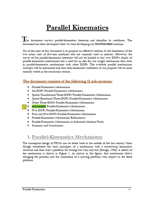
_______________________________________________________________________________________ Parallel Kinematics 12P a r a l l e l K i n e m a t i c shis document surveys parallel-kinematics literature and identifies its usefulness. Thedocument has been developed while we were developing our SimParallel machine.On of the aims of this document is to propose an effective solution to the limitations of thetwo rotary axes of five-axis machines that are currently used in industry. However, thesurvey of the parallel-kinematics literature will not be limited to this (two DOFs) family ofparallel kinematics mechanisms lest a seed for an idea for our sought mechanism does existin parallel-kinematics mechanisms with other DOFs. The available parallel mechanismsconcepts will be mentioned and then their kinematics usefulness to our purpose will be morecritically stated in the conclusion section.The document consists of the following 11 sub-sections;•Parallel-Kinematics Mechanisms. •Six DOFs Parallel-Kinematics Mechanisms. •Spatial Translational Three-DOFs Parallel-Kinematics Mechanisms. •Spatial Rotational Three-DOFs Parallel-Kinematics Mechanisms. • Other Three-DOFs Parallel-Kinematics Mechanisms.•Asymmetric Parallel-Kinematics Mechanisms. •Two DOFs Parallel-Kinematics Mechanisms. •Four and Five-DOFs Parallel-Kinematics Mechanisms. •Parallel-Kinematics Mechanisms Redundancy. •Parallel-Kinematics Mechanisms in Industrial Machine-Tools. •Summary and Conclusions1. Parallel-Kinematics MechanismsThe conceptual design of PKMs can be dated back to the middle of the last century whenGough established the basic principles of a mechanism with a closed-loop kinematicsstructure and then built a platform for testing tyre wear and tear [Gough, 1956]. A sketch ofthe mechanism is shown in Figure 1. As shown in the figure, that mechanism allowschanging the position and the orientation of a moving platform with respect to the fixedplatform.T______________________________________________________________________________________ Parallel Kinematics 13Later in 1965 Stewart designed another parallel-kinematics platform for use as an aircraftsimulator [Stewart, 1965]. A sketch of that Stewart mechanism is shown in Figure 2. Forsome reason the mechanisms of Figure 1 and that of Figure 2 as well as many variations (e.g.the one shown in Figure 3 ) are frequently called in the literature Stewart platform. They arealso called Hexapod mechanisms.Figure 2 Stewart Platform Figure 1Gough Platform______________________________________________________________________________________Parallel Kinematics 14Of course other mechanisms related, may be less formally, to PKM existed well before andsoon before Gough’s platform. Bonev [2003] surveyed many of these earlier mechanisms.Gough though is the one who gave some formalization to the concept. It might beinteresting to know that Gough’s platform remained operational till year 1998 and it is nowkept at the British National Museum of Science and Industry. See Figure 4 for photos of theoriginal and current shapes of Gough platform.Many have extensively analyzed Gough/Hexapod platform [Hunt, 1983, Fichter 1986,Griffis and Duffy, 1989; Wohlhart, 1994]. One problem with these six-DOFs platforms isthe difficulty of their forward-kinematics solution, because of the nonlinearity and the highlycoupled nature of their governing equations. This difficulty has been overcome byintroducing some assumptions [Zhang and Song, 1994] and a closed-form solutiuon can befound in [Wen and Liang, 1994]. Others introduced some sensors to measure at least one ofFigure 4Old and Revived Gough Platform Figure 3 Gough-Stewart-Hexapod Platformthe variables of the platform and hence reduce the unknowns of the governing equations[Merlet, 1993; Bonev et al, 1999]. The above mechanisms are six DOFs mechanisms becauseeach of them allows the moving platform to move arbitrarily (within the limit of the work-space) in the six DOF space.Having had a look on the mechanisms above one can now introduce a formal definition ofparallel-kinematics mechanisms; A parallel-kinematics mechanism (or parallel manipulator) isa closed-loop mechanism. That is, a moving plate (ie end-effector) is connected to thestationary base by at least two independent kinematic chains, each of which is actuated. Onthe other hand, A serial-kinematics mechanism (or serial manipulator) is an open-loopmechanism in which each link is connected to ONLY two neighbouring links. All themechanisms discussed in the introduction of Chapter 1 are serial-kinematics mechanisms.The advantages of parallel-kinematics mechanisms in general are;•Excellent load/weight ratios, as a number of kinematic chains are sharing the load.•High stiffness, as the kinematics chains (limbs) are sharing loads and in many cases the links can be designed such that they are exposed to tensile and compressive loadsonly [Hunt, 1978]. This high stiffness insures that the deformations of the links willbe minimal and this feature greatly contributes to the high positioning accuracy ofthe manipulator.•Low inertia, because most of the actuators are attached to the base, and thus no heavy mass need to be moved.•The position of the end-effector is not sensitive to the error on the articular sensors.Higher accuracy due to non-cumulative joint error.•Many different designs of parallel manipulators are possible and the scientific literature on this topic is very rich, as will be shown later in this chapter.•The mechanisms are of low cost since most of the components are standard.•Usually, all actuators can be located on the fixed platform.•Work-space is easily accessible.•The possibility of using these mechanisms as a 6-component force-sensor. Indeed it can be shown that the measurement of the traction-compression stress in the linksenables to calculate the forces and torques acting on the mobile platform. This isespecially useful in haptic devices [Tsumaki et al, 1998].On the other hand, the disadvantages of parallel-kinematics mechanisms in general are;•For many configurations there are some analytical difficulties ( eg the forward kinematics solution is not easy or finding all the mechanism singularities can beextremely difficult task).•The need in many cases for the expensive spherical joints.•Limited useful work-space compared to the mechanism size.•Limited dexterity.•Scaling up PKMs can enlarge the translational DOFs and usually is unable to enlarge the rotational DOFs.•Potential mechanical-design difficulty.•Mechanism assembly has to be done with care.•Time-consuming calibration might be necessary. See [Ryu and Abdul-rauf, 2001] to realize that calibration of PKMs is not a trivial issue.______________________________________________________________________________________ Parallel Kinematics 15______________________________________________________________________________________Parallel Kinematics 16Many other different points of view about the benefits of PKMs and their drawbacks can befound in the literature [Brogårdh, 2002].2. Six-DOFs PKMsThe PKMs mentioned in the previous section are six-DOFs PKMs. Some of thesemechanisms have S-P-S kinematics chains. S-P-S chains are preferred as they, as discussed inAppendix A, transmit no torque through the limbs. These PKMs can also be realized usingS-P-U chains or any other chain that has six-DOFs associated with its joints. One can checkthat against Grübler/Kutzbach criterion above, or review Appendix A. In fact acomprehensive attempt to enumerate the joints combinations and permutations that can beutilized when all the limbs are identical has been reported [Tsai, 1998]. It can also be shownthat the DOFs associated with the limbs joints need to be at least six. See Appendix A too.Figure 5 shows one PKM that has been proposed. It uses six P-R-U-U limbs [Wiegand et al,1996]. Similar to the PKMs above this one also has limited tilting ability. The reachabletilting angle changes strongly with the position of the P joints and fluctuates between 20 and45 degrees. In special poses up to 57 degrees can be reached.It is important to notice that changing the number of limbs in symmetrical six-DOFs PKMswill not change the DOFs of the platform. This has been shown using Grübler/Kutzbachcriterion in Appendix A, and also can be observed in Figure 6 to Figure 9. In these examplesthough we need more than one actuator per limb, and if there are less than six actuatorssome of the DOFs will not be controllable.A Symmetrical PKM is one that has identical kinematics chains (also called limbs or legs)each of which utilize identical actuator.Figure 6 shows another six-DOFs PKM [Tsai and Tahmasebi, 1993]. This PKM has three P-P-S-R limbs. However, planar motors can not provide high load-carrying capacity and theyoccupy the whole base leaving no space to the material to be processed. A similar PKM waslater built and studied [Ben-Horin et al, 1996]. Figure 7 shows a PKM with three P-P-R-Slimbs [Kim and Park, 1998; Ryu et al, 1998]. The range of tilting angles of the platform ofthis mechanism is one of the widest that can found in the literature. However, themechanism uses 8 actuators (for the six P joints and two of the R joints) to realize themotion that can be realized with six actuators only, and many translational motions can beFigure 5 Six-DOFs PKM withsix P-S-U limbs______________________________________________________________________________________ Parallel Kinematics 17realized in direct straight lines. A PKM similar to that shown in Figure 7 has been proposedearlier [Alizade and Tagiyev, 1994]. That earlier PKM had three P-R-P-S limbs instead.Figure 6 Six-DOFs PKM with three P-P-S-R chains Figure 7 Six-DOFs PKM with three P-P-R-S chains Figure 8 Six-DOFs PKM using three Scott mechanisms( b ) ( c )______________________________________________________________________________________Parallel Kinematics 18Probably no mechanism is more famous than the single DOF crank-slider of Figure 8.a. It isa P-R-R-R kinematic chain that coverts linear to rotary motion or vice versa. Scott’smechanism of Figure 8.b [Khurmi and Gupta, 1985] is another traditional planar mechanismthat greatly resembles the well known crank-slider mechanism. Three of these Scottmechanisms have been put together, as shown in Figure 8.c, to realize a three-DOFsmechanism and then each of the Scott mechanism was made to displace vertically, resultingin a six-DOFs mechanism [Zabalza et al l, 2002]. Some of the R joints of the originalmechanism have been replaced by S joints to allow spatial motion of the arms. Theadvantage of the concept is that if one attempts to express the position and the orientationof the platform via its three vertices, then the kinematics relations will be fairly decoupled.The PKMs of Figure 6 and Figure 7 could be considered decoupled. Other six-DOFsdecoupled PKMs have also been proposed [Zlatanov et al. 1992; Wohlhart, 1994].Spherical actuators that can provide three-DOFs actuation are expensive and notcommercially available [Williams and Poling, 2000], but if two of these actuators are used theGough-Stewart platform of Figure 3 can be reduced to the one shown in Figure 9. Pendingthe quality and the mechanical characteristics of these spherical actuators, the solution offersan elegant and promising solution. The work-space, as least the translational part of it, is stilllimited though and load is shared between two rather than six limbs.Six-DOFs PKMs represent the roots of the concept of PKMs and hence they had to belooked at. However, one might say that a six DOFs PKM is PKMs at their extreme, andconsequently one might think that reducing the number of DOFs that act in parallel mightalleviate the disadvantages of parallel-kinematics mechanisms while benefiting from theiradvantages. This is actually true in many cases. In trials to avoid the disadvantages of sixDOFs parallel-kinematics mechanisms while utilizing the other benefits of parallel-kinematics mechanisms, two, three, four and five DOFs PKMs were proposed, as will beshown in the subsequent sections.3. Spatial Translational Three-DOFs PKMsThree-DOFs PKMs for pure rotation or pure translation are of special importance as theyare, in our view, represent a low-level entity or building block of PKMs that helps deepeningthe understanding of these mechanisms. One can subsequently hybridize these two buildingFigure 9 Six-DOFs PKM with two S-P-U Chains______________________________________________________________________________________ Parallel Kinematics 19blocks or sub-systems from them. Spatial translational three-DOFs PKMs are discussed inthis section and spatial rotational three-DOFs PKMs are discussed in the next section.Using Grübler/Kutzbach criterion one can see that using three limbs (legs) each having five-DOFs is one way to realize three-DOFs symmetrical PKMs. See Appendix A for examples.Many of such PKMs have been built and Figure 10 to Figure 13 show examples of thisfamily of translational three-DOFs PKMs. That is, Figure 10 shows a PKM with three limbseach with U-P-U joints [Tsai, 1996]. This mechanism has been studied by others [DiGregorio and Parenti-Castelli, 1998] and been further optimized [Tsai and Joshi, 2000] andits mobility also has been discussed in details [Di Gregorio and Parenti-Castelli, 2002].Obviously the same kind of motion can also be obtained using P-U-U kinematic chains[Tasora et al, 2001], as shown in Figure 11.Figure 10 Translational U-P-U PKM Figure 11 Translational P-U-U PKM______________________________________________________________________________________Parallel Kinematics 20One should notice that the U-P-U mechanism is a special case from the R-R-P-R-Rmechanism, when the axes of each R-R pairs are perpendicular. This R-R-P-R-R has beenstudied and the conditions that need to be satisfied to enable its pure translational motionhas been established [Di Gregorio and Parenti-Castelli,1998]. The P joints can also bereplaced by R joints and the result is shown in Figure 12 [Tsai, 1999]. Alternatively one ofthe R joints could be replaced by P joints resulting in R-P-R-P-R (or R-C-C; C forCylindrical) [Callegari and Marzitti, 2003]. This is shown in Figure 13.In fact all the combinations and permutations the basic R and/or P joints that would resultin PKMs with three five-DOFs limbs have been enumerated [Tsai, 1998; Kong andGosselin, 2001]. Notice that if pure translation is sought using symmetrical PKMs, then Sjoints would not be a favorable choice as one S joint in each limb simply means that rotationcannot be constrained.The Delta mechanism [Clavel, 1988] is one of the earliest and the most famous spatialtranslational three-DOFs parallel-kinematics robots, as it has been marketed and usedindustrially for pick and place applications. A sketch of this mechanism is shown in Figure14. This mechanism can provide pure 3D translational motion to its moving platform usingits three rotary actuators via its three limbs. Each of these limbs actually is a R-R-Pa-RFigure 12 Translational R-U-U PKM Figure 13 Translational R-P-R-P-R (R-C-C) PKM______________________________________________________________________________________ Parallel Kinematics 21 (Revolute-Revolute-Parallelogram-Revolute) kinematic chain. The mechanism can alsoprovide a rotary independent motion about the Z axis as a 4th decoupled DOF.Many variations of that Delta mechanism has been proposed and implemented. One ofthese close variations is the patented Tsai’s manipulator [ Tsai, 1997; Stamper 1997 ], whichalso provides 3D translational motion to its platform. Here, the parallelograms areconstructed using R joints instead of S joints and Stirrups in the previous case. Thatmechanism is shown in Figure 15. Another close variation was also presented [Mitova andVatkitchev, 1991]. The kinematic chains of that variation were R-Pa-R-R instead.A P-R-Pa-R with vertical prismatic joints was also suggested [Zobel et al, 1996]. Variationsextremely similar to that were later implemented using pneumatic drives [Kuhlbusch andNeumann, 2002]. These variations are shown in Figure 16.Figure 14Clavel-Delta translational PKMFigure 15Tsai or Meryland translationalPKM______________________________________________________________________________________When the lines of action of the three prismatic joints are tilted further till all of them are inthe horizontal plane, the star mechanism of Figure 17 is then obtained. This mechanism wasdeveloped by Hervé [Hervé and Sparacino, 1992]. Notice here that the prismatic joints arereplaced by helical ones (ie screw & nut), which should not represent a difference fromkinematics points of view.Figure 16Translational P-R-Pa-R PKMs Figure 17 Herve ’ Star translational PKM Figure 18 The Orthoglide translational PKM ( a ) ( b )( c )______________________________________________________________________________________ Parallel Kinematics 23 The orthoglide mechanism [Wenger and Chablat, 2000 and 2002] is another variation withthe angles between the action lines of the prismatic joints are changed further resulting inbetter motion transformation (from joints to platform) quality. This is shown in Figure 18.Prior to that a similar mechanism has also been designed and built as a coordinate-measuring-machine [Hiraki et al, 1997]. In that mechanism the lines of action of theprismatic joints are changed further to guarantee that the heavy parts if the mechanism areresting on the machine base.Parallelograms represent a common thread among the mechanisms of Figure 14 to Figure 18as a parallelogram would directly constrain the rotational motion about certain axis. SeeAppendix A. Notice also that in all the designs above the two axes of the two revolute jointsof each chain are always parallel, sometimes parallel to the direction of the prismatic joint (ifany) and sometimes perpendicular to it, which agrees with conditions shown later in theliterature [Kong and Gosselin, 2004b].It is important to notice that each limb of each of the PKMs of Figure 14 to Figure 18 hasonly four-DOFs associated with its joints. According to Grübler/Kutzbach criterion thesePKMs are not mobile [Stamper, 1997]. In fact some mechanisms are mobile only undersome geometric conditions. These are called internally over-constrained mechanisms. SeeAppendix A for more about these over-constrained mechanisms. Screw theory can beutilized in conjunction with the Grübler/Kutzbach criterion [Huang and Li, 2002] to showthe mobility of these over-constrained mechanisms.Further, other (that do not utilize parallelograms) spatial translational PKMs with three limbseach of which having four-DOFs have been proposed. Symmetrical PKMs that have three(P-R-R-R) limbs and are aimed at realizing pure spatial translational motion have been built[Kong and Gosselin, 2002a; Kong and Gosselin, 2002b]. Two of these PKMs are shown inFigure 19. For these over-constrained PKMs to realize pure translation the followinggeometrical conditions need to be satisfied;• The axes of the 3 R joints within the same limb are parallel.• The three directions of the R joints of the limbs should not be in the same plane orparallel to the same plane.• Within the same leg the axis of the P joint is not perpendicular to the direction of the R joints axes.Figure 19 Translational Over-Constrained P-R-R-R PKMThe directions of the P joints don’t have to be parallel, but if they are this will help enlarging the work-space. Also, it has been shown that if the three directions of the R joints are perpendicular to each other linear isotropic transformations will be obtained throughout the work-space (and thus no singularities). Compare that to the isotropic conditions reported for the orthoglide mechanism of Figure 18. Isotropic transformation is discussed further in Chapter 4.The geometrical conditions of the mobility of a similar over-constrained PKMs that has three C-P-R (P-R-P-R) limbs, shown in Figure 20, have also been found [Callegari and Tarantini, 2003]. These conditions are;•The axes of the 2 R joints within the same limb are parallel.•The three directions of the R joints of the three limbs should not be in the same plane or parallel to the same plane.It has been shown that singularity of that mechanism can be kept outside the work-space while maintaining a convex work-space. The isotropic points of that mechanism have also been shown.Figure 20Translational Over-ConstrainedP-R-P-R Symmetrical PKMIn fact the geometrical conditions of the different over-constrained PKMs that utilize four-DOFs limbs have been enumerated [Hervé and Sparacino, 1991; Kong and Gosselin, 2004a].Using three limbs each with P-P-P joints is actually another, may be trivial, over-constrained translational PKMs.Another concept that has been extensively utilized at the industrial level is presented now. If three limbs each with six-DOFs (eg U-P-S kinematic chain) associated with its joints are used, then the platform will have six DOFs (as discussed in Appendix A). However, if less than six actuators are used with these three limbs then some DOFs will not be controllable.After choosing which DOFs are to be controlled, one can compensate for the known but uncontrolled motion of the remaining DOFs using other, may be serial, mechanism. One can also use some limbs to mechanically constraint some of the platform DOFs. In fact this is the basic idea behind Neumann’s patented mechanism [Neumann, 1988] of Figure 21.This seems like creating some DOFs that are needed and then constraining or compensating for them. Still, the idea has been utilized. Various aspects of this PKM has been studied extensively [eg Siciliano, 1999] and a further utilization of the concept will be shown in a subsequent section of this chapter. One might say or think that this concept/mechanism is actually is under-utilization of resources because of a prior conviction to utilize a Gough-like platform/limbs.____________________________________________________________________________________________________________________________________________________________________________ Parallel Kinematics 254. Spatial Rotational Three-DOFs PKMsExactly as in the case of spatial translational three-DOFs PKMs spatial rotational three-DOFs PKMs can be realized using three limbs each with five-DOFs associated with itsjoints. The difference now is how the joints of the PKM would be assembled. A PKM withthree U-P-U limbs, just like the one discuused in conjunction with Figure 10, has beenproposed [Karouia, and Hervé, 2000]. Another PKM with three R-R-S (or R-S-R) limbs, asshown in Figure 22, has also been proposed [Karouia, and Hervé, 2002a]. PKM with threeR-U-U have also been presented as well [Hervé and Karouia, 2002b]. Figure 23 also showshow to use three P-R-P-R-R (or C-P-U) limbs to realize a spherical/rotation three-DOFsPKMs [Callegari et al 2004]. PKMs with three U-R-C and with three R-R-S legs have beenproposed as well [Di Gregorio, 2001; Di Gregorio, 2002]. A PKM that utilizesparallelograms (similar to the delta PKM above) within its three R-Pa-S limbs was yetanother propsoed spehrical PKM [Vischer and Clavel, 2000]. In fact the possible sphericalPKMs that are based on five-DOFs limbs are enumerated [Kong and Gosselin 2004b; Kong and Gosselin 2004c; Karouia, and Hervé, 2002b; Karouia, and Hervé, 2003].Figure 21 Neumann ’s constrained U-P-S PKM Synthesis of three-DOFs translational PKMs based on either Lie/Displacement group theory [Hervé and Sparacino, 1991; Hervè, 1999] or on screw theory [Tsai, 1999; Kong and Gosselin, 2004a] have been discussed. Figure 22 Orientation R-S-E PKM______________________________________________________________________________________Again, as in the translational case, over-constrained PKMs can be used to realizeorientational PKMs. If only R joints are used then three R-R-R legs can be used [Gosselinand Angeles, 1989]. The geometric condition that will mobilize this over-constrained PKM isthat all the axes of the used R joints are to be concurrent at the rotation center of themechanism. See Figure 24. Figure 25 shows one of these R-R-R limbs separately. Notice thatin this case the space freedom ( λ ) is three as no element of the mechanism is translating,which should simplify the application of Grübler/Kutzbach criterion. Notice also that onlytwo R-R-R legs can theoretically be used to realize a three-DOFs rotational PKM. SeeAppendix A. This is not usually favorable though as one actuator will not be placed on thePKM base. For isotropic transformation the axes of the R joints of each limb should beperpendicular to each other [Wiitala and Stanisi ć, 2000].Figure 24 Orientation R-R-R over-constrained PKM Figure 25 Orientation R-R-R limb Figure 23 Orientation C-P-U PKMWhen P joints are used then four-DOFs legs can be used to realize over-constrainedrotational PKMs [Kong and Gosselin, 2004c]. The combinations and permutations ofpossible over-constrained spherical PKMs as well as their necessary geometrical conditionsare enumerated [Kong and Gosselin, 2004b; Kong and Gosselin, 2004c].As happened in the translational case using Neumann’s PKM of Figure 21, three six-DOFslegs can be used to realize a six-DOFs PKM and then mechanically constrain thetranslational DOFs. The limbs used can have kinematic structure of P-U-S or R-U-S or theirvariations, as per Figure 26. In these cases an arm extending from the base is used topivot/constrain the platform. The P-U-S or R-U-S chains can theoretically be replaced by S-P-S chain, which also has six DOFs associated with its joints [Mohammadi et al, 1993], asshown in Figure 27.( a ) ( b)( c)Figure 26Orientation U-P-S or R-U-S PKMFigure 27Orientation S-P-S PKM______________________________________________________________________________________ Parallel Kinematics 27Type synthesis of three-DOFs rotational PKMs based on either Lie/Displacement group theory [Karouia and Hervé, 2003] or on screw theory [Kong and Gosselin, 2004b] have been discussed.5.Other Three-DOFs PKMsSo far spatial three DOFs mechanisms have been discussed. Three DOFs mechanisms can provide planar motion too. That is, they can provide the platform with two translational motions and one rotational motion about the plane normal. If, one relies on P and/or R joints as well as Grübler/Kutzbach criterion, then one can find that there are 7 possible symmetrical mechanisms. These are (RRR, RRP, RPR, PRR, RPP PRP, and PPR). S and U joints here not useful here. Each of the three identical kinematic chains in this case needs to have 3 DOFs [Tsai, 1998]. Figure 28 [Hunt, 1983] and Figure 29 [Tsai, 1998] represent two of these possible seven mechanisms that have actually been implemented.Figure 28Planar R-R-R PKMFigure 29Planar P-R-P PKMFigure 30Planar PKM with three PRR limbsor redundancyThe mechanism of Figure 30 is another planar symmetrical 3 DOF PKM that has been proposed [Marquet et al, 2001]. Three P-R-R limbs are used. In the figure one can actually see a 4th chain. This is actually a redundant one to treat singularity, which will be discussed in Section 7. With this fourth P-R-R limb P-U-S limbs have also been proposed.Planar PKMs cannot provide two spatial rotational DOFs and hence they can not directly serve the purpose of this work, and hence they are surveyed thoroughly. Other PKMs can ______________________________________________________________________________________。

abaqus结构分析单元类型

a b a q u s结构分析单元类型(总5页)--本页仅作为文档封面，使用时请直接删除即可----内页可以根据需求调整合适字体及大小--;this wordfile adds the code folding function which is useful to ignore rows of numbers,enjoy~;updated in , based on the wordfile "abaqus_67ef()";Syntax file for abaqus keywords ,code folding enabled;add *ANISOTROPIC *ENRICHMENT *LOW -DISPLACEMENT HYPERELASTIC;newly add /C"ElementType";delete DISPLACEMENT;delete MASS in /C2"Keywords2"/L29"abaqus_612" Nocase File Extensions = inp des dat msg/Delimiters = ~!@$%^&()_-+=|\/{}[]:;"'<> ,.//Function String = "%[ ^t]++[ps][a-z]+ [a-z0-9]+ ^(*(*)^)*{$"/Function String 1 = "%[ ^t]++[ps][a-z]+ [a-z0-9]+ ^(*(*)^)[ ^t]++$" /Member String = "^([A-Za-z0-9_:.]+^)[ ^t*&]+$S[ ^t]++[(=);,]"/Variable String = "^([A-Za-z0-9_:.]+^)[ ^t*&]+$S[ ^t]++[(=);,]"/Open Fold Strings = "*" "**""***"/Close Fold Strings = "*" "**""***"/C1"Keywords1" STYLE_KEYWORD*ACOUSTIC *ADAPTIVE *AMPLITUDE *ANISOTROPIC *ANNEAL *AQUA *ASSEMBLY *ASYMMETRIC *AXIAL *BASE *BASELINE *BEAM*BIAXIAL *BLOCKAGE *BOND *BOUNDARY *BRITTLE *BUCKLE *BUCKLING *BULK *C *CAP *CAPACITY *CAST *CAVITY *CECHARGE*CECURRENT *CENTROID *CFILM *CFLOW *CFLUX *CHANGE *CLAY *CLEARANCE*CLOAD *CO *COHESIVE *COMBINED *COMPLEX*CONCRETE *CONDUCTIVITY *CONNECTOR *CONSTRAINT *CONTACT *CONTOUR*CONTROLS *CORRELATION *COUPLED *COUPLING*CRADIATE *CREEP *CRUSHABLE *CYCLED *CYCLIC *D *DAMAGE *DAMPING*DASHPOT *DEBOND *DECHARGE *DECURRENT*DEFORMATION *DENSITY *DEPVAR *DESIGN *DETONATION *DFLOW *DFLUX*DIAGNOSTICS *DIELECTRIC *DIFFUSIVITY*DIRECT *DISPLAY *DISTRIBUTING *DISTRIBUTION *DLOAD *DRAG *DRUCKER*DSA *DSECHARGE *DSECURRENT *DSFLOW*DSFLUX *DSLOAD *DYNAMIC *EL *ELASTIC *ELCOPY *ELECTRICAL *ELEMENT*ELGEN *ELSET *EMBEDDED *EMISSIVITY*END *ENERGY *ENRICHMENT *EOS *EPJOINT *EQUATION *EULERIAN *EXPANSION *EXTREME *FABRIC *FAIL *FAILURE*FASTENER *FIELD *FILE *FILM *FILTER *FIXED *FLOW *FLUID *FOUNDATION *FRACTURE *FRAME *FREQUENCY *FRICTION*GAP *GASKET *GEL *GEOSTATIC *GLOBAL *HEADING *HEAT *HEATCAP*HOURGLASS *HYPERELASTIC *HYPERFOAM *HYPOELASTIC*HYSTERESIS *IMPEDANCE *IMPERFECTION *IMPORT *INCIDENT *INCLUDE*INCREMENTATION *INELASTIC *INERTIA*INITIAL *INSTANCE *INTEGRATED *INTERACTION *INTERFACE *ITS *JOINT*JOINTED *JOULE *KAPPA *KINEMATIC*LATENT *LOAD *LOADING *LOW *M1 *M2 *MAP *MASS *MATERIAL *MATRIX*MEMBRANE *MODAL *MODEL *MOHR *MOISTURE*MOLECULAR *MONITOR *MOTION *MPC *MULLINS *NCOPY *NFILL *NGEN *NMAP *NO *NODAL *NODE *NONSTRUCTURAL*NORMAL *NSET *ORIENTATION *ORNL *OUTPUT *PARAMETER *PART *PERIODIC *PERMEABILITY *PHYSICAL *PIEZOELECTRIC*PIPE *PLANAR *PLASTIC *POROUS *POST *POTENTIAL *PRE *PREPRINT*PRESSURE *PRESTRESS *PRINT *PSD *RADIATE*RADIATION *RANDOM *RATE *RATIOS *REBAR *REFLECTION *RELEASE*RESPONSE *RESTART *RETAINED *RIGID *ROTARY*SECTION *SELECT *SFILM *SFLOW *SHEAR *SHELL *SIMPEDANCE *SIMPLE*SLIDE *SLOAD *SOILS *SOLID *SOLUBILITY*SOLUTION *SOLVER *SORPTION *SPECIFIC *SPECTRUM *SPRING *SRADIATE*STATIC *STEADY *STEP *SUBMODEL*SUBSTRUCTURE *SURFACE *SWELLING *SYMMETRIC *SYSTEM *TEMPERATURE*TENSILE *TENSION *THERMAL *TIE *TIME*TORQUE *TRACER *TRANSFORM *TRANSPORT *TRANSVERSE *TRIAXIAL *TRS *UEL *UNDEX *UNIAXIAL *UNLOADING *USER*VARIABLE *VIEWFACTOR *VISCO *VISCOELASTIC *VISCOUS *VOID *VOLUMETRIC *WAVE *WIND-AXISYMMETRIC -DEFINITION -DISPLACEMENT -SIMULATION -SOIL -TENSION/C2"Keywords2"ACTIVATION ADDED AREA ASSEMBLE ASSEMBLY ASSIGNMENT AXIALBEHAVIOR BODY BULKCASE CAVITY CENTER CHAIN CHANGE CHARGE CLEARANCE COMPACTION COMPONENT COMPRESSION CONDITIONS CONDUCTANCECONDUCTIVITY CONSTANTS CONSTITUTIVE CONSTRAINT CONTACT CONTROL CONTROLS COPY CORRECTION COULOMB COUPLINGCRACKING CREEP CRITERIA CRITERION CYCLICDAMAGE DAMAGED DAMPING DATA DEFINED DEFINITION DELETE DENSITY DEPENDENCE DEPENDENT DERIVED DETECTIONDIFFUSION DIRECTORY DOFS DYNAMIC DYNAMICSEFFECT EIGENMODES ELASTIC ELASTICITY ELECTRICAL ELEMENT ELSET ENVELOPE EVOLUTION EXCHANGE EXCLUSIONSEXPANSIONFACTORS FAILURE FIELD FILE FLAW FLOW FLUID FLUX FOAM FORMAT FORMULATION FRACTION FREQUENCY FRICTIONGENERAL GENERATE GENERATION GRADIENTHARDENING HEAT HOLD HYPERELASTICINCLUSIONS INERTIA INFLATOR INITIATION INPUT INSTANCE INTEGRAL INTERACTION INTERFERENCE IRONLAYER LEAKOFF LENGTH LINE LINK LOAD LOCKM1 M2 MATERIAL MATRIX MEDIUM MESH METAL MIXTURE MODEL MODES MODULI MODULUS MOTIONNODAL NODE NSET NUCLEATIONORIGIN OUTPUTPAIR PARAMETER PART PARTICLE PATH PENETRATION PLASTIC PLASTICITY POINT POINTS POTENTIAL PRAGER PRINTPROPERTYRADIATION RATE RATIOS REDUCTION REFERENCE REFLECTION REGION RELIEF RESPONSE RESULTS RETENTIONSECTION SCALING SHAPE SHEAR SOLID SOLUTION SPECTRUM STABILIZATION STATE STEP STIFFENING STIFFNESS STOPSTRAIN STRESS SURFACE SWELLING SYMMETRYTABLE TECHNIQUE TEMPERATURE TENSION TEST THERMAL THICKNESS TO TORQUE TRANSFER TRANSPORTVALUE VARIABLES VARIATION VELOCITY VIEWFACTOR VISCOSITYWAVE WEIGHT/C3"ElementType" STYLE_ELEMENTAC1D2 AC1D3 AC2D3 AC2D4 AC2D4R AC2D6 AC2D8 AC3D4 AC3D6 AC3D8 AC3D8R AC3D10 AC3D15 AC3D20 ACAX3 ACAX4ACAX4R ACAX6 ACAX8 ACIN2D2 ACIN2D3 ACIN3D3 ACIN3D4 ACIN3D6 ACIN3D8 ACINAX2 ACINAX3 ASI1 ASI2 ASI2AASI2D2 ASI2D3 ASI3 ASI3A ASI3D3 ASI3D4 ASI3D6 ASI3D8 ASI4 ASI8 ASIAX2 ASIAX3B21 B21H B22 B22H B23 B23H B31 B31H B31OS B31OSH B32 B32H B32OSB32OSH B33 B33HC3D4 C3D4E C3D4H C3D4P C3D4T C3D6 C3D6E C3D6H C3D6P C3D6T C3D8 C3D8E C3D8H C3D8HT C3D8I C3D8IH C3D8PC3D8PH C3D8PHT C3D8PT C3D8R C3D8RH C3D8RHT C3D8RP C3D8RPH C3D8RPHTC3D8RPT C3D8RT C3D8T C3D10 C3D10EC3D10H C3D10I C3D10M C3D10MH C3D10MHT C3D10MP C3D10MPH C3D10MPTC3D10MT C3D15 C3D15E C3D15H C3D15VC3D15VH C3D20 C3D20E C3D20H C3D20HT C3D20P C3D20PH C3D20R C3D20REC3D20RH C3D20RHT C3D20RP C3D20RPHC3D20RT C3D20T C3D27 C3D27H C3D27R C3D27RH CAX3 CAX3E CAX3H CAX3T CAX4 CAX4E CAX4H CAX4HT CAX4ICAX4IH CAX4P CAX4PH CAX4PT CAX4R CAX4RH CAX4RHT CAX4RP CAX4RPHCAX4RPHT CAX4RPT CAX4RT CAX4T CAX6CAX6E CAX6H CAX6M CAX6MH CAX6MHT CAX6MP CAX6MPH CAX6MT CAX8 CAX8E CAX8H CAX8HT CAX8P CAX8PH CAX8RCAX8RE CAX8RH CAX8RHT CAX8RP CAX8RPH CAX8RT CAX8T CAXA4HN CAXA4N CAXA4RHN CAXA4RN CAXA8HN CAXA8NCAXA8PN CAXA8RHN CAXA8RN CAXA8RPN CCL12 CCL12H CCL18 CCL18H CCL24 CCL24H CCL24R CCL24RH CCL9 CCL9HCGAX3 CGAX3H CGAX3HT CGAX3T CGAX4 CGAX4H CGAX4HT CGAX4R CGAX4RH CGAX4RHT CGAX4RT CGAX4T CGAX6 CGAX6HCGAX6M CGAX6MH CGAX6MHT CGAX6MT CGAX8 CGAX8H CGAX8HT CGAX8R CGAX8RH CGAX8RHT CGAX8RT CGAX8T CIN3D12RCIN3D18R CIN3D8 CINAX4 CINAX5R CINPE4 CINPE5R CINPS4 CINPS5R COH2D4 COH2D4P COH3D6 COH3D6P COH3D8COH3D8P COHAX4 COHAX4P CONN2D2 CONN3D2 CPE3 CPE3E CPE3H CPE3T CPE4 CPE4E CPE4H CPE4HT CPE4I CPE4IHCPE4P CPE4PH CPE4R CPE4RH CPE4RHT CPE4RP CPE4RPH CPE4RT CPE4T CPE6 CPE6E CPE6H CPE6M CPE6MH CPE6MHTCPE6MP CPE6MPH CPE6MT CPE8 CPE8E CPE8H CPE8HT CPE8P CPE8PH CPE8RCPE8RE CPE8RH CPE8RHT CPE8RPCPE8RPH CPE8RT CPE8T CPEG3 CPEG3H CPEG3HT CPEG3T CPEG4 CPEG4H CPEG4HT CPEG4I CPEG4IH CPEG4R CPEG4RHCPEG4RHT CPEG4RT CPEG4T CPEG6 CPEG6H CPEG6M CPEG6MH CPEG6MHT CPEG6MT CPEG8 CPEG8H CPEG8HT CPEG8RCPEG8RH CPEG8RHT CPEG8T CPS3 CPS3E CPS3T CPS4 CPS4E CPS4I CPS4RCPS4RT CPS4T CPS6 CPS6E CPS6M CPS6MTCPS8 CPS8E CPS8R CPS8RE CPS8RT CPS8TDASHPOT1 DASHPOT2 DASHPOTA DC1D2 DC1D2E DC1D3 DC1D3E DC2D3 DC2D3EDC2D4 DC2D4E DC2D6 DC2D6E DC2D8DC2D8E DC3D10 DC3D10E DC3D15 DC3D15E DC3D20 DC3D20E DC3D4 DC3D4EDC3D6 DC3D6E DC3D8 DC3D8E DCAX3DCAX3E DCAX4 DCAX4E DCAX6 DCAX6E DCAX8 DCAX8E DCC1D2 DCC1D2D DCC2D4 DCC2D4D DCC3D8 DCC3D8D DCCAX2DCCAX2D DCCAX4 DCCAX4D DCOUP2D DCOUP3D DGAP DRAG2D DRAG3D DS3 DS4 DS6 DS8 DSAX1 DSAX2EC3D8R EC3D8RT ELBOW31 ELBOW31B ELBOW31C ELBOW32 EMC2D3 EMC2D4 EMC3D4 EMC3D8F2D2 F3D3 F3D4 FAX2 FLINK FRAME2D FRAME3D FC3D4 FC3D6 FC3D8GAPCYL GAPSPHER GAPUNI GAPUNIT GK2D2 GK2D2N GK3D12M GK3D12MN GK3D18 GK3D18N GK3D2 GK3D2N GK3D4LGK3D4LN GK3D6 GK3D6L GK3D6LN GK3D6N GK3D8 GK3D8N GKAX2 GKAX2N GKAX4 GKAX4N GKAX6 GKAX6N GKPE4 GKPE6GKPS4 GKPS4N GKPS6 GKPS6NHEATCAPIRS21A IRS22A ISL21A ISL22A ITSCYL ITSUNI ITT21 ITT31JOINT2D JOINT3D JOINTCLS3S LS6MASS M3D3 M3D4 M3D4R M3D6 M3D8 M3D8R M3D9 M3D9R MAX1 MAX2 MCL6 MCL9 MGAX1 MGAX2PC3D PIPE21 PIPE21H PIPE22 PIPE22H PIPE31 PIPE31H PIPE32 PIPE32HPSI24 PSI26 PSI34 PSI36Q3D4 Q3D6 Q3D8 Q3D8H Q3D8R Q3D8RH Q3D10M Q3D10MH Q3D20 Q3D20H Q3D20R Q3D20RHR2D2 R3D3 R3D4 RAX2 RB2D2 RB3D2 ROTARYIS3 S3T S3R S3RS S3RT S4 S4T S4R S4RT S4R5 S4RS S4RSW S8R S8R5 S8RT S9R5 SAX1 SAX2 SAX2T SAXA1NSAXA2N SC6R SC6RT SC8R SC8RT SFM3D3 SFM3D4 SFM3D4R SFM3D6 SFM3D8 SFM3D8R SFMAX1 SFMAX2 SFMCL6 SFMCL9SFMGAX1 SFMGAX2 SPRING1 SPRING2 SPRINGA STRI3 STRI65T2D2 T2D2E T2D2H T2D2T T2D3 T2D3E T2D3H T2D3T T3D2 T3D2E T3D2H T3D2T T3D3 T3D3E T3D3H T3D3TWARP2D3 WARP2D4。

基于运动学正解的Delta机器人工作空间分析

Ｍ＝６×(１７－２１－１) ＋３×６＋１５＝３
２ ቤተ መጻሕፍቲ ባይዱｅｌｔａ机器人的运动学模型
２.１Ｄｅｌｔａ机器人的运动学逆解
机器人的运动学逆解是已知机器人末端在参考坐标系的位姿Ｔ的情况下ꎬ求机器人各个关节变量ｑｉ的取值ꎮ 运动学的逆解是控制机器人的关键ꎬ因为只有各关节变量
作者简介:韦岩(１９９２－) ꎬ男ꎬ江苏沭阳人ꎬ硕士研究生ꎬ研究方向为机电系统集成与机器人控制ꎮ
Ｋｅｙｗｏｒｄｓ:ＭｏｎｔｅＣａｒｌｏｍｅｔｈｏｄꎻ Ｄｅｌｔａｒｏｂｏｔꎻ ｗｏｒｋｓｐａｃｅꎻ ｋｉｎｅｍａｔｉｃｓ
０引言
广义的并联机械臂是末端的执行装置由几个独立的运动支链连接到基座ꎬ形成的闭环运动链机构[１] ꎮ 瑞士的Ｒｅｙｍｏｎｄｃｌａｖｅｌ教授于１９８５年提出的Ｄｅｌｔａ机器人是应用最为广泛的并联机构之一ꎮ 由于Ｄｅｌｔａ机器人的结构特点ꎬ使它只有３个平移自由度ꎬ设计、制造、控制都比较简便ꎬ在轻工业分拣与包装中应用广泛ꎮ 机器人的工作空间是衡量机器人工作性能的一个重要性能指标ꎬ在进行机构设计、控制、轨迹规划时ꎬ工作空间是首先必须要考虑的重要问题ꎮ 本文介绍一种Ｄｅｌｔａ机器人的结构及工作原理ꎬ使用蒙特卡罗方法ꎬ在位置正解的基础上ꎬ结合ＭＡＴ￣ＬＡＢ软件对工作空间进行探索研究ꎮ
ＷｏｒｋｓｐａｃｅＡｎａｌｙｓｉｓｏｆＤｅｌｔａＲｏｂｏｔＢａｓｅｄｏｎＦｏｒｗａｒｄＫｉｎｅｍａｔｉｃｓ
ＷＥＩＹａｎꎬ ＬＩＲａｎｒａｎꎬ ＺＨＡＮＧＬｕｈａｏꎬ ＺＨＯＵＷａｎｌｉꎬ ＹＵＨａｎｑｉ ( ＩｎｄｕｓｔｒｉａｌＣｅｎｔｅｒꎬ ＮａｎｊｉｎｇＩｎｓｔｉｔｕｔｅｏｆＴｅｃｈｎｏｌｏｇｙꎬ Ｎａｎｊｉｎｇ２１１１６７ꎬＣｈｉｎａ) Ａｂｓｔｒａｃｔ:Ｂａｓｅｄｏｎｔｈｅｔｈｅｏｒｙｏｆｐａｒａｌｌｅｌｒｏｂｏｔｍｅｃｈａｎｉｓｍꎬ ｔｈｉｓｐａｐｅｒａｎａｌｙｓｅｓｔｈｅｐｏｓｉｔｉｏｎｏｆＤｅｌｔａｒｏｂｏｔｍｅｃｈａｎｉｓｍꎬ ｅｓｔａｂｌｉｓｈｅｓ

合驱动机构运动学分析

南京航空航天大学硕士学位论文合驱动机构运动学分析姓名：彭于华申请学位级别：硕士专业：机械电子工程指导教师：吴洪涛2010-12南京航空航天大学硕士学位论文摘要随着现代工业的飞速发展，对锻压生产提出的要求也越来越高。

通用机械压力机主要采用曲柄连杆机构作为主传动机构，由于其机械特性的限制，在工作时，噪声和振动大且模具寿命低。

本文根据江苏某公司的要求，研究用六连杆机构替代曲柄滑块机构的可行性并分析了其运动特性，同时对当前压力机领域比较热门的混合驱动压力机进行了部分研究，本文主要的工作内容如下：1)阐述了课题来源及课题的研究背景，简述了压力机的发展历程，综述了国内外相关领域的研究现状并指出了本文的主要研究内容。

2)首先选定多连杆驱动机构为六连杆机构，利用复数矢量法，对六连杆机构进行运动学分析，讲述运动学分析的意义并从运动学的角度分析塑性加工对压力机运动学特征的要求。

给出机构位移、速度、加速度矢量方程的推导过程，再采用数学软件Mathematica的强大的符号推导功能，利用其复数包能方便的得出运动学解析解，并利用Mechanical System包得出六连杆机构的运动曲线。

3)应用机械系统运动学/动力学仿真分析软件ADAMS建立六连杆压力机执行机构的虚拟样机模型，然后利用ADAMS中的优化功能对机构进行优化分析，选定设计变量，并确定目标函数和约束条件，避免了繁杂的编程过程，提高了分析效率和质量，最终得到最优化的各杆尺寸，并将优化前后的结果进行了对比。

4)根据的最优化实体尺寸，设计了六连杆压力机的结构布置，并在Pro/E中完成了六连杆压力机的三维实体建模及装配建模，给出了六连杆压力机的内部结构图和多点成形六连杆压力机的内部传动原理，同时简单介绍了几个关键零部件的建模思路及技巧。

5)将机架导入ANSYS，利用Ansys建立其有限元模型并对其进行了静态分析，得出了机架各部分结构的应力和变形云图，为以后对机架的进一步优化提供了基础。

Kinematic Optimization Robot Alignment

Kinematic Optimization Robot Alignment As a robot, I understand the importance of kinematic optimization in robot alignment. This process is crucial for ensuring that robots can perform their tasks with precision and efficiency. However, achieving optimal robot alignment can be a complex and challenging task that requires careful consideration of various factors. In this response, I will discuss the importance of kinematic optimization in robot alignment, the challenges associated with this process, and potential solutions to improve the alignment of robots.First and foremost, it is important to recognize the significance of kinematic optimization in robot alignment. When a robot is properly aligned, it can perform its tasks with a high degree of accuracy and repeatability. This is essential in various industries, such as manufacturing, where precision is critical for producing high-quality products. Additionally, optimal robot alignment can also contribute to increased safety in the workplace, as it reduces the likelihood of errors and accidents.Despite the importance of kinematic optimization, achieving optimal robot alignment can be challenging. One of the primary challenges is the complexity of the robot's kinematic structure. Robots often have multiple joints and links, which can result in a high degree of freedom. As a result, determining the optimal configuration of these joints to achieve a specific end-effector position and orientation can be a complex mathematical problem. Additionally, factors such as mechanical tolerances, wear and tear, and environmental conditions can further complicate the alignment process.Another challenge in robot alignment is the need for precise calibration and measurement. In order to optimize the kinematics of a robot, accurate data regarding the robot's physical structure and behavior is essential. However, obtaining this data can be challenging, as it often requires advanced measurement techniques and equipment. Furthermore, the process of calibrating a robot can be time-consuming and labor-intensive, requiring careful adjustments to ensure that the robot's kinematic model accurately reflects its physical behavior.In light of these challenges, it is important to consider potential solutions to improve the alignment of robots. One potential solution is the use of advanced sensing and measurement technologies. For example, the integration of high-precision sensors and cameras can facilitate the accurate measurement of a robot's position, orientation, and other relevant parameters. Additionally, the use of advanced algorithms and software tools can help analyze this data and optimize the robot's kinematic configuration.Furthermore, advancements in robotics technology, such as the development of more sophisticated actuators and control systems, can also contribute to improved robot alignment. For example, the use of high-performance actuators with built-in feedback mechanisms can enhance the robot's ability to achieve and maintain precise alignment. Similarly, the integration of advanced control algorithms can enable robots to adapt to changes in their environment and maintain optimal alignment in real-time.In conclusion, kinematic optimization is a critical aspect of robot alignment that has significant implications for the performance and safety of robots in various industries. However, achieving optimal robot alignment can be a complex and challenging task, given the inherent complexity of robot kinematics and the need for precise calibration and measurement. Nevertheless, by leveraging advanced sensing and measurement technologies, as well as advancements in robotics technology, it is possible to improve the alignment of robots and enhance their capabilities. Ultimately, the pursuit of optimal robot alignment is essential for realizing the full potential of robotics in the modern world.。

机械专业外文翻译-挖掘机的机械学和液压学

┊┊┊┊┊┊┊┊┊┊┊┊┊装┊┊┊┊┊订┊┊┊┊┊线┊┊┊┊┊┊┊┊┊┊┊┊┊Multi-Domain Simulation:Mechanics and Hydraulics of an Excavator Abstract It is demonstrated how to model and simulate an excavator with Modelica and Dymola by using Modelica libraries for multi-body and for hydraulic systems. The hydraulic system is controlled by a “load sensing” controller. Usually, models containing3-dimensional mechanical and hydraulic components are difficult to simulate. At hand of the excavator it is shown that Modelica is well suited for such kinds of system simulations.1. IntroductionThe design of a new product requires a number of decisions in the initial phase that severely affect the success of the finished machine. Today, digital simulation is therefore used in early stages to look at different concepts. The view of this paper is that a new excavator is to be designed and several candidates of hydraulic control systems have to be evaluated.Systems that consist of 3-dimensional mechanical and of hydraulic components – like excavators – are difficult to simulate. Usually, two different simulation environments have to be coupled. This is often inconvenient, leads to unnecessary numerical problems and has fragile interfaces. In this article it is demonstrated at hand of the model of an excavator that Modelica is well suited for these types of systems.The 3-dimensional components of the excavator are modeled with the new, free Modelica MultiBody library. This allows especially to use an analytic solution of the kinematic loop at the bucket and to take the masses of the hydraulic cylinders, i.e., the “force elements”, directly into account. The hydraulic part is modeled in a detailed way, utilizing pump, valves and cylinders from HyLib, a hydraulics library for Modelica. For the control part a generic “load sensing” control system is used, modeled by a set of simple equations. This approach gives the required results and keeps the time needed for analyzing the problem on a reasonable level.2. Modeling ChoicesThere are several approaches when simulating a system. Depending on the task it may be necessary to build a very precise model, containing every detail of the system and needing a lot of information, e.g., model parameters. This kind of models is expensive to build up but on the other hand very useful if parameters of a well defined system have to be modified. A typical example is the optimization of parameters of a counterbalance valve in an excavator (Kraft 1996).The other kind of model is needed for a first study of a system. In this case some properties of the pump, cylinders and loads are specified. Required is information about the performance of that system, e.g., the speed of the pistons or the necessary input power at the pump shaft, to make a decision whether this design can be used in principle for the task at hand. This model has therefore to be “cheap”, i.e., it must be possible to build it in a short time without detailed knowledge of particular components.The authors intended to build up a model of the second type, run it and have first results with a minimum amount of time spent. To achieve this goal the modeling language Modelica (Modelica 2002), the Modelica simulation environment Dymola (Dymola 2003), the new Modelica library for 3-dimensional mechanical systems “MultiBody”(Otter et al. 2003) and the Modelica library of hydraulic components HyLib (Beater 2000) was used. The model consists of the 3-dimensional mechanical construction of the excavator, a detailed description of the power hydraulics and a generic “load sensing” controller. This model will be available as a demo in the next version of HyLib.3. Construction of ExcavatorsIn Figure 1 a schematic drawing of a typical excavator under consideration is shown. It consists of a chain track and the hydraulic propel drive which is used to manoeuvre the machine but usually not during a work cycle. On top of that is a carriage where the operator is sitting. It can rotate around a vertical axis with respect to the chain track. It also holds the Diesel engine, the hydraulic pumps and control system. Furthermore, there is a boom, an arm and at the end a bucket which is attached via a planar kinematic loop to the arm. Boom, arm and bucket can be rotated by the appropriate cylinders.┊┊┊┊┊┊┊┊┊┊┊┊┊装┊┊┊┊┊订┊┊┊┊┊线┊┊┊┊┊┊┊┊┊┊┊┊┊Figure 2 shows that the required pressures in the cylinders depend on the position. For the “stretched” situation the pressure in the boom cylinder is 60 % higher than in the retracted position. Not only the position but also the movements have to be taken into account. Figure 3 shows a situation where the arm hangs down. If the carriage does not rotate there is a pulling force required in the cylinder. When rotating –excavators can typically rotate with up to 12 revolutions per minute –the force in the arm cylinder changes its sign and now a pushing force is needed. This change is very significant because now the “active” chamber of the cylinder switches and that must be taken into account by the control system. Both figures demonstrate that a simulation model must take into account the couplings between the four degrees of freedom this excavator has. A simpler model that uses a constant load for each cylinder and the swivel drive leads to erroneous results4. Load Sensing SystemExcavators have typically one Diesel engine, two hydraulic motors and three cylinders. There exist different hydraulic circuits to provide the consumers with the required hydraulic energy. A typical design is a Load Sensing circuit that is energy efficient and user friendly. The idea is to have a flow rate control system for the pump such that it delivers exactly the needed flow rate. As a sensor the pressure drop across an orifice is used. The reference value is the resistance of the orifice. A schematic drawing is shown in figure 4, a good introduction to that topic is given in (anon. 1992).The pump control valve maintains a pressure at the pump port that is typically 15 bar higher than the pressure in the LS line (= Load Sensing line). If the directional valve is closed the pump has therefore a stand-by pressure of 15 bar. If it is open the pump delivers a flow rate that leads to a pressure drop of 15 bar across that directional valve. Note: The directional valve is not used to throttle the pump flow but as a flow meter (pressure drop that is fed back) and as a reference (resistance). The circuit is energy efficient because the pump delivers only the needed flow rate, the throttling losses are small compared to other circuits.If more than one cylinder is used the circuit becomes more complicated, see figure 5. E.g. if the boom requires a pressure of 100 bar and the bucket a pressure of 300 bar the pump pressure must be above 300 bar which would cause an unwanted movement of the boom cylinder. Therefore compensators are used that throttle the oil flow and thus achieve a pressure drop of 15 bar across the particular directional valve. These compensators can be installed upstream or downstream of the directional valves. An additional valve reduces the nominal pressure differential if the maximum pump flow rate or the maximum pressure is reached (see e.g. Nikolaus 1994).5. Model of Mechanical PartIn Figure 6, a Modelica schematic of the mechanical part is shown. The chain track is not modeled, i.e., it is assumed that the chain track does not move. Components “rev1”, ..., “rev4” are the 4 revolute joints to move the parts relative to each other. The icons with the long black line are “virtual”rods that are used to mark specific points on a part, especially the mounting points of the hydraulic cylinders. The light blue spheres (b2, b3, b4, b5) are bodies that have mass and an inertia tensor and are used to model the corresponding properties of the excavator parts.The three components “cyl1f”, “cyl2f”,and “cyl3f” are line force components that describe a force interaction along a line between two attachment points. The small green squares at these components represent 1-dimensional translational connectors from theModelica.Mechanics. Translational library. They are used to define the 1- dimensional force law acting between the two attachment points. Here, the hydraulic cylinders described in the next section are directly attached. The small two spheres in the icons of the “cyl1f,cyl2f, cyl3f” components indicate that optionally two point masses are taken into account that are attached at defined distances from the attachment points along the connecting line. This allows to easily model the essential mass properties (mass and center of mass) of the hydraulic cylinders with only a very small computational overhead.The jointRRR component (see right part of Figure 6) is an assembly element consisting of 3 revolute joints that form together a planar loop when connected to the arm. A picture of this part of an excavator, a zoom in the corresponding Modelica schematic and the animation view is shown in Figure 7. When moving revolute joint “rev4” (= the large red cylinder in the lower part of Figure 7; the small┊┊┊┊┊┊┊┊┊┊┊┊┊装┊┊┊┊┊订┊┊┊┊┊线┊┊┊┊┊┊┊┊┊┊┊┊┊red cylinders characterize the 3 revolute joints of the jointRRR assembly component) the position and orientation of the attachment points of the “left”and “right” revolute joints of the jointRRR component are known. There is a non-linear algebraic loop in the jointRRR component to compute the angles of its three revolute joints given the movement of these attachment points. This non-linear system of equations is solved analytically in the jointRRR object, i.e., in a robust and efficient way. For details see In a first step, the mechanical part of the excavator is simulated without the hydraulic system to test this part separatly. This is performed by attaching translational springs with appropriate spring constants instead of the hydraulic cylinders. After the animation looks fine and the forces and torques in the joints have the expected size, the springs are replaced by the hydraulic system described in the next sections.All components of the new MultiBody library have “built-in” animation definitions, i.e., animation properties are mostly deduced by default from the given definition of the multi-body system. For example, a rod connecting two revolute joints is by default visualized as cylinder where the diameter d is a fraction of the cylinder length L (d = L/40) which is in turn given by the distance of the two revolute joints. A revolute joint is by default visualized by a red cylinder directed along the axis of rotation of the joint. The default animation (with only a few minor adaptations) of the excavator is shown if Figure 8. The light blue spheres characterize the center of mass of bodies. The line force elements that visualize the hydraulic cylinders are defined by two cylinders (yellow and grey color) that are moving in each other. As can be seen, the default animation is useful to get, without extra work from the user side, a rough picture of the model that allows to check the most important properties visually, e.g., whether the center of masses or attachment points are at the expected places.For every component the default animation can be switched off via a Boolean flag. Removing appropriate default animations, such as the “centerof- mass s pheres”, and adding some components that have pure visual information (all visXXX components in the schematic of Figure 6) gives quickly a nicer animation, as is demonstrated in Figure 9. Also CAD data could be utilized for the animation, but this was not available for the examination of this excavator.6. The Hydraulics Library HyLibThe (commercial) Modelica library HyLib (Beater 2000, HyLib 2003) is used to model the pump, metering orifice, load compensator and cylinder of the hydraulic circuit. All these components are standard components for hydraulic circuits and can be obtained from many manufacturers. Models of all of them are contained in HyLib. These mathematical models include both standard textbook models (e. g. Dransfield 1981, Merrit 1967, Viersma 1980) and the most advanced published models that take the behavior of real components into account (Schulz 1979, Will 1968). An example is the general pump model where the output flow is reduced if pressure at the inlet port falls below atmospheric pressure. Numerical properties were also considered when selecting a model (Beater 1999). One point worth mentioning is the fact that all models can be viewed at source code level and are documented by approx. 100 references from easily available literature.After opening the library, the main window is displayed (Figure 10). A double click on the “pumps” icon opens the selection for all components that are needed to originate or end an oil flow (Figure 11). For the problem at hand, a hydraulic flow source with internal leakage and externally commanded flow rate is used. Similarly the needed models for the valves, cylinders and other components are chosen.All components are modeled hierarchically. Starting with a definition of a connector –a port were the oil enters or leaves the component – a template for components with two ports is written. This can be inherited for ideal models, e.g., a laminar resistance or a pressure relief valve. While it usually makes sense to use textual input for these basic models most of the main library models were programmed graphically, i.e., composed from basic library models using the graphical user interface. Figure12 gives an example of graphical programming. All mentioned components were chosen from the library and then graphically connected.7. Library Components in Hydraulics CircuitThe composition diagram in Figure 12 shows the graphically composed hydraulics part of the excavator model. The sub models are chosen from the appropriate libraries, connected and the┊┊┊┊┊┊┊┊┊┊┊┊┊装┊┊┊┊┊订┊┊┊┊┊线┊┊┊┊┊┊┊┊┊┊┊┊┊parameters input. Note that the cylinders and the motor from HyLib can be simply connected to the also shown components of the MultiBody library. The input signals, i.e., the reference signals of the driver of the excavator, are given by tables, specifying the diameter of the metering orifice, i.e. the reference value for the flow rate. From the mechanical part of the excavator only the components are shown in Figure 12 that are directly coupled with hydraulic elements, such as line force elements to which the hydraulic cylinders are attached.8. Model of LS ControlFor this study the following approach is chosen: Model the mechanics of the excavator, the cylinders and to a certain extent the pump and metering valves in detail because only the parameters of the components will be changed, the general structure is fixed. This means that the diameter of the bucket cylinder may be changed but there will be exactly one cylinder working as shown in Figure 1. That is different for the rest of the hydraulic system. In this paper a Load Sensing system, or LS system for short, using one pump is shown but there are other concepts that have to be evaluated during an initial design phase. For instance the use of two pumps, or a separate pump for the swing.The hydraulic control system can be set up using meshed control loops. As there is (almost) no way to implement phase shifting behavior in purely hydraulic control systems the following generic LS system uses only proportional controllers.A detailed model based on actual components would be much bigger and is usually not available at the begin of an initial design phase. It could be built with the components from the hydraulics library but would require a considerable amount of time that is usually not available at the beginning of a project.In Tables 1 and 2, the implementation of the LS control in form of equations is shown. Usually, it is recommended for Modelica models to either use graphical model decomposition or to define the model by equations, but not to mix both descrip- tion forms on the same model level.For the LS system this is different because it has 17 input signals and 5 output signals. One might built one block with 17 inputs and 5 outputs and connect them to the hydraulic circuit. However, in this case it seems more understandable to provide the equations directly on the same level as the hydraulic circuit above and access the input and output signals directly. For example, ”metOri1.port_A.p” used in table 2 is the measured pressure at port_A of the metering orifice metOri1. The calculated values of the LS controller, e.g., the pump flow rate “pump.inPort.signal[1] = ...” is the signal at the filled blue rectangle of the “pump” component, see Figure 12).The strong point of Modelica is that a seamless integration of the 3-dimensional mechanical library, the hydraulics library and the non standard, and therefore in no library available, model of the control system is easily done. The library components can be graphically connected in the object diagram and the text based model can access all needed variables.9. Some Simulation ResultsThe complete model was built using the Modelica modeling and simulation environment Dymola (Dymola 2003), translated, compiled and simulated for 5 s. The simulation time was 17 s using the DASSL integrator with a relative tolerance of 10-6 on a 1.8 GHz notebook, i.e., about 3.4 times slower as real-time. The animation feature in Dymola makes it possible to view the movements in an almost realistic way which helps to explain the results also to non-experts, see Figure 9.Figure 13 gives the reference signals for the three cylinders and the swing, the pump flow rate and pressure. From t = 1.1 s until 1.7 s and from t = 3.6 s until 4.0 s the pump delivers the maximum flow rate. From t = 3.1 s until 3.6 s the maximum allowed pressure is reached. Figure 14 gives the position of the boom and the bucket cylinders and the swing angle. It can be seen that there is no significant change in the piston movement if another movement starts or ends. The control system reduces the couplings between the consumers which are very severe for simple throttling control.Figure 15 shows the operation of the bucket cylinder. The top figure shows the reference trajectory, i. e. the opening of the directional valve. The middle figure shows the conductance of the compensators. With the exception of two spikes it is open from t = 0 s until t = 1 s. This means that in┊┊┊┊┊┊┊┊┊┊┊┊┊装┊┊┊┊┊订┊┊┊┊┊线┊┊┊┊┊┊┊┊┊┊┊┊┊that interval the pump pressure is commanded by that bucket cylinder. After t = 1 s the boom cylinder requires a considerably higher pressure and the bucket compensator therefore increases the resistance (smaller conductance). The bottom figure shows that the flow rate control works fine. Even though there is a severe disturbance (high pump pressure after t = 1 s due to the boom) the commanded flow rate is fed with a small error to the bucket cylinder.10. ConclusionFor the evaluation of different hydraulic circuits a dynamic model of an excavator was built. It consists of a detailed model of the 3 dimensional mechanics of the carriage, including boom, arm and bucket and the standard hydraulic components like pump or cylinder. The control system was not modeled on a component basis but the system was described by a set of nonlinear equations.The system was modeled using the Modelica MultiBody library, the hydraulics library Hylib and a set of application specific equations. With the tool Dymola the system could be build and tested in a short time and it was possible to calculate the required trajectories for evaluation of the control system.The animation feature in Dymola makes it possible to view the movements in an almost realistic way which helps to explain the results also to多畴模拟：挖掘机的机械学和液压学概要：通过使用用于多体和液压系统的Modelica程序库，示范通过Modelica和Dymola如何模拟和仿真挖掘机。

1、下载文档前请自行甄别文档内容的完整性，平台不提供额外的编辑、内容补充、找答案等附加服务。
2、"仅部分预览"的文档,不可在线预览部分如存在完整性等问题,可反馈申请退款(可完整预览的文档不适用该条件!)。
3、如文档侵犯您的权益，请联系客服反馈,我们会尽快为您处理(人工客服工作时间：9:00-18:30)。

model are obtained through obtaining relationships between the input joint angles and the output position/orientation information of the end-effector. For example, in [6], feedforward neural network has been used to model the forward kinematics of Steward platform. Backpropagation learning strategy was used to train the network which resulted in a model where the forward solutions were accurate within a ﬁnite bound. An improved strategy was then proposed by using mapping offset adjustment, which gave better mapping results on the training data set. However, no generalization results from testing set of data were presented. In [7], polynomial networks were used to model the forward kinematics of parallel manipulators, testing was carried out on a circular trajectories. For the case of parallel spherical manipulator, it was found that this model is not suitable for the laparoscopic surgery application, since the end effector of the device needs to be positioned in any arbitrary conﬁguration in the work space instead of following a given trajectory. Furthermore, no experimental studies have been reported in previous works such as [6] and [7]. The spherical parallel mechanism is designed as a haptic device and has been used as an educational environment for laparoscopes surgery in the Experimental Robotics Laboratory at Simon Fraser University. For this real time surgery training application, a model of forward kinematics is needed to interface the haptic device and the graphic model. There are two tasks we need to consider for this application, one is to model the forward kinematics, and the other task is to implement the model to the environment for the real time application. The relationship of these two tasks is shown in Fig.1. The objective of this paper is to model the forward kinematics of the haptic device using neural networks. The goal of modelling is to map the motor angles to position and orientation of end effector in its work space. The training data for the networks are collected either from inverse kinematics model or directly from a experimental prototype of the mechanism. Three motor angles are read from the encoders of these motors through the computer interface. Levenberg-Marquardt algorithm is used to train the networks. After training, a NN model will be obtained and can be used for the real time implementation. II. S TRUCTURE AND KINEMATICS OF PARALLEL
NN-based solution of forward kinematics of 3DOF parallel spherical manipulator
Temei Li, Qingguo Li and Shahram Payendeh Experimental Robotics Laboratory(ERL), School of Engineering Science Simon Fraser University 8888 University Drive Burntly, B.C., Canada V5A 1S6
I. INTRODUCTION The parallel manipulator was ﬁrst proposed by Stewart in 1965 as an aircraft simulator platform[1]. The spherical parallel mechanisms have been also studied as haptic devices to train surgeons or as tele-surgery mechanism with three degree of freedom (DOF) for laparoscopic surgery[2]. In laparoscopic surgery, surgeons manipulate long surgical tools to complete procedures such as executional, ablative, and reconstructive base on complexity. Surgeons are required to practice and trained considerably in order to acquire complex surgical skills. In design of haptic training environment, it is required to develop an electromechanical device which offers similar motion as that in the actual surgery. For this purpoeds to be developed. In general, the inverse kinematics for the parallel spherical mechanism is unique and can be easily computed. For forward kinematic problem, closed form solutions are only available for special conﬁgurations of parallel manipulators[3]. The lack of a closed form solution and the nonlinearity of the forward kinematic problem has been offering some unique challenges for parallel manipulator researchers[4]. In order to solve the forward kinematics, numerical methods have been implemented to solve the nonlinear equations. In general, this class of approaches are computationally time consuming. In our surgery training environment application, it requires a real time solution, so this approach is not suitable. Other approaches for solving the forward kinematic problems are based on learning methods. In this class of methods, the forward kinematic
Abstract— In this paper, neural networks are trained to compute the forward kinematics of spherical parallel manipulator(PM) for laparoscopic surgery application. Instead of solving a set of nonlinear equations for the forward kinematics, neural networks are used to map the input angles of revolute joints to the orientation of the manipulator. The training data are obtained from inverse kinematic relationships and measured from the experimental prototype model of the manipulator. LevenbergMarquardt algorithm is used to train the neural networks, which leads to the fast convergence of the networks. The trained neural network model of forward kinametics are used in the real time interface between the graphical model and a haptic device for the laparoscopes surgery training application. Simulation and experiments are carried out to verify the performance of the proposed method. Index Terms— Kinematics, parallel manipulators, neural networks, laparoscopic surgery