Generic Aggregated Wind Farm Model for Power System Simulations
AGPRIS V2.0 农业生产性空间模拟软件说明书

Package‘AGPRIS’June8,2023Title AGricultural PRoductivity in SpaceVersion2.0DescriptionFunctionalities to simulate space-time data and to estimate dynamic-spatial panel data models.Estimators implemented are the BCML(El-horst(2010),<doi:10.1016/j.regsciurbeco.2010.03.003>),the MML(El-horst(2010)<doi:10.1016/j.regsciurbeco.2010.03.003>)and the INLA Bayesian estima-tor(Lindgren and Rue,(2015)<doi:10.18637/jss.v063.i19>;Bivand,Gomez-Rubio and Rue,(2015)<doi:10.18637/jss.v063.i20>)adapted to panel data.The package contains functions to replicate the analyses of the scien-tific article entitled``Agricultural Productivity in Space''(Baldoni and Es-posti(2021),<doi:10.1111/ajae.12155>)).License GPL-3Encoding UTF-8LazyData trueRoxygenNote7.1.1Depends R(>=2.10)Imports methods,Matrix,plyr,sp,spdep,spacetime,matrixcalc,maxLikSuggests INLA,terraNeedsCompilation noAuthor Edoardo Baldoni[aut,cre](<https:///0000-0002-5296-1212>)Maintainer Edoardo Baldoni<*************************>Repository CRANDate/Publication2023-06-0807:32:54UTCR topics documented:bcml (2)distOte (3)inla.st (4)12bcml map1 (5)map2 (6)map3 (6)map4 (7)mml (7)r100km (8)r20km (9)r40km (9)r60km (10)regsamp (10)sel_regioni (11)sim_data_fe (11)tabSard (12)Index14 bcml BCML estimatorDescriptionThis function estimates a space time linear model according to the specified formula.It implements the BCML(or BCLSDV)estimator as in Elhorst(2010)doi:10.1016/j.regsciurbeco.2010.03.003. Usagebcml(dataset,yearStart,yearEnd,var.agg="Cod_Provincia",eq,spatial=NULL,estimation="analytical",corrBIAS=TRUE,WMAT=NULL)Argumentsdataset STFDF with the datayearStart First year considered in the estimationyearEnd Last Anno considered in the estimationvar.agg Index of the spatial unitseq Formula to be estimated.It excludes the spatial lagspatial Radius to define neighborsdistOte3 estimation Either’analytical’or’numerical’.If’analytical’is specified the concentrated maximum likelihood is estimated and then the other parameters are obtainedanalytically.Otherwise,all parameters are obtained through numerical maxi-mization of the log-likelihood function.corrBIAS Boolean.If TRUE,the bias correction is applied.WMAT The spatial weight matrixValueA list with two objects.Thefirst object is the estimates table.The second object is the log-likelihoodevaluated at its maximumExampleslibrary(maxLik)library(matrixcalc)set.seed(123)sd=sim_data_fe(dataset=regsamp,N=100,TT=8,spatial=80,Tau=-0.2,Rho=0.4,Beta=2,sdDev=2,startingT=10,LONGLAT=TRUE)est_bcml=bcml(dataset=sd[[1]],yearStart=3,yearEnd=9,var.agg= Cod_Provincia ,eq=Y~X1,estimation= analytical ,corrBIAS=TRUE,WMAT=sd[[2]]) est_bcmldistOte Matrix of technological distanceDescriptionA matrix of agricultural technological distance of NUTS3.It is used to weight the geographicaldistance of NUTS3regions.UsagedistOteFormatA106x106matrix4inla.st inla.st Space-time bayesian INLA estimatorDescriptionThis function estimates a space time linear model using the bayesian INLA.It is a wrapper of the INLA::inla function(Lindgren and Rue(2015)doi:10.18637/jss.v063.i19;Bivand,Gomez-Rubio and Rue(2015)doi:10.18637/jss.v063.i20)adapted to panel data.Usageinla.st(formula,d,W,RHO,PHI,var.agg,normalization=FALSE,improve=TRUE,fhyper=NULL,probit=FALSE,...)Argumentsformula Formula of the model to be estimatedd Data frameW Spatial matrixRHO Parameter of spatial dependencePHI Parameter of temporal dependencevar.agg Indexes of the panel dimensions.Thefirst argument is the spatial dimension, the second argument is the temporal dimension.normalization Boolean.If TRUE the data are normalized before estimationimprove Please refer to the documentation of the INLA packagefhyper Plase refer to the documentation of the INLA packageprobit Plase refer to the documentation of the INLA package...additional parameters.Please,refer to the documentation of the INLA package ValueReturns a model of class"inla".Please,refer to the documentation of the INLA package for addi-tional informationExampleslibrary(terra)set.seed(123)sd=sim_data_fe(dataset=regsamp,N=100,TT=8,spatial=80,Tau=-0.2,Rho=0.4,Beta=2,sdDev=2,startingT=10,LONGLAT=TRUE)est_inla=inla.st(formula=Y~-1+X1,d=sd[[1]]@data,W=sd[[2]],PHI=-0.2,RHO=0.4,var.agg=c( Cod_Provincia , Anno ),family= gaussian ,improve=TRUE,normalization=FALSE,control.family=list(hyper=list(prec=list(initial=25,fixed=TRUE))),control.predictor=list(compute=TRUE),pute=list(dic=TRUE,cpo=TRUE),control.inla=list(print.joint.hyper=TRUE))summary(est_inla)map1Cropland grid of Northen Italy(20km x20km squares)DescriptionSpatialPolygonsDataFrame object with croplands of Northern Italy approximated with20km x 20km squared polygons.It is based on croplands data contained in the Corine Land Cover2012 raster map.Usagemap1FormatSpatialPolygonsDataFrame objectSourcehttps://land.copernicus.eu/pan-european/corine-land-cover/clc-2012map2Cropland grid of Northen Italy(40km x40km squares)DescriptionSpatialPolygonsDataFrame object with croplands of Northern Italy approximated with40km x 40km squared polygons.It is based on croplands data contained in the Corine Land Cover2012 raster map.Usagemap2FormatSpatialPolygonsDataFrame objectSourcehttps://land.copernicus.eu/pan-european/corine-land-cover/clc-2012map3Cropland grid of Northen Italy(60km x60km squares)DescriptionSpatialPolygonsDataFrame object with croplands of Northern Italy approximated with60km x 60km squared polygons.It is based on croplands data contained in the Corine Land Cover2012 raster map.Usagemap3FormatSpatialPolygonsDataFrame objectSourcehttps://land.copernicus.eu/pan-european/corine-land-cover/clc-2012map4Cropland grid of Northen Italy(100km x100km squares)DescriptionSpatialPolygonsDataFrame object with croplands of Northern Italy approximated with100km x 100km squared polygons.It is based on croplands data contained in the Corine Land Cover2012 raster map.Usagemap4FormatSpatialPolygonsDataFrame objectSourcehttps://land.copernicus.eu/pan-european/corine-land-cover/clc-2012mml MML estimatorDescriptionThis function estimates a space time linear model according to the specified formula using the ML estimator as in Elhorst(2010)doi:10.1016/j.regsciurbeco.2010.03.003.The estimator maximizes the full log-likelihood function in which the parameter of spatial dependence is constrained. Usagemml(Rho,ff,dataset,wmat,var.agg,m=10)ArgumentsRho the constrained parameter of spatial dependenceff Formula of the linear model.It excludes the spatial lagdataset Data frame with the datawmat Spatial weight matrixvar.agg Spatial index of the data framem How many time periods have passed since the beginning of the space-time pro-cess8r100km ValueThe estimates tablesExamplesset.seed(123)sd=sim_data_fe(dataset=regsamp,N=50,TT=6,spatial=80,Tau=-0.2,Rho=0.4,Beta=2,sdDev=2,startingT=10,LONGLAT=TRUE);sd[[1]]$X2=stats::rnorm(nrow(sd[[1]]@data)) est_mml=mml(dataset=sd[[1]]@data,Rho=0.4,ff=Y~X1+X2,wmat=sd[[2]],var.agg=c( Anno , Cod_Provincia ),m=10)est_mmlr100km Cropland grid of Italy(100km x100km squares)DescriptionSpatialPolygonsDataFrame object with croplands of Italy approximated with100km x100km squared polygons.It is based on croplands data contained in the Corine Land Cover2012raster map.Usager100kmFormatSpatialPolygonsDataFrame objectSourcehttps://land.copernicus.eu/pan-european/corine-land-cover/clc-2012r20km9 r20km Cropland grid of Italy(20km x20km squares)DescriptionSpatialPolygonsDataFrame object with croplands of Italy approximated with20km x20km squared polygons.It is based on croplands data contained in the Corine Land Cover2012raster map. Usager20kmFormatSpatialPolygonsDataFrame objectSourcehttps://land.copernicus.eu/pan-european/corine-land-cover/clc-2012r40km Cropland grid of Italy(40km x40km squares)DescriptionSpatialPolygonsDataFrame object with croplands of Italy approximated with40km x40km squared polygons.It is based on croplands data contained in the Corine Land Cover2012raster map. Usager40kmFormatSpatialPolygonsDataFrame objectSourcehttps://land.copernicus.eu/pan-european/corine-land-cover/clc-201210regsamp r60km Cropland grid of Italy(60km x60km squares)DescriptionSpatialPolygonsDataFrame object with croplands of Italy approximated with60km x60km squared polygons.It is based on croplands data contained in the Corine Land Cover2012raster map. Usager60kmFormatSpatialPolygonsDataFrame objectSourcehttps://land.copernicus.eu/pan-european/corine-land-cover/clc-2012regsamp Coordinates of simulated farms in Northern ItalyDescriptionSpatialPointsDataFrame object with1000SpatialPoints to represent simulated farms in the simula-tion exerciseUsageregsampFormatSpatialPointsDataFrame objectsel_regioni11 sel_regioni Merged NUTS3for simulation exerciseDescriptionSpatialPolygons object with merged NUTS3regions of Northern Italy used in the simulation exer-ciseUsagesel_regioniFormatSpatialPolygons objectSourceISTATsim_data_fe Simulate space-time stochastic process withfixed-effectDescriptionThis function simulates a space-time stochastic process according to the defined spatial structure and input paramters.It simulates data of a dynamic spatial lag model.It includes one exogenous variable and afixed-effect correlated with the exogenous variable.Usagesim_data_fe(dataset,N,TT,spatial=100,Tau=-0.14,Rho=0.67,Beta=1,sdDev=5,startingT=11,LONGLAT=TRUE)Argumentsdataset SpatialObject with the spatial units for which the data will be simulatedN How many spatial units will be usedTT Time dimension of the simulated processspatial Radius that defines the scope of spatial dependenceTau Autocorrelation parameterRho Spatial dependence parameterBeta Coefficient associated to the exogenous variablesdDev Standard Deviation of the(gaussian)error termstartingT The number of time periods after which the simulated data will be recorded LONGLAT Boolean.If the projection is longlatValueA list with two objects.Thefirst object is the STFDF with the simulated data.The second object isthe spatial weight matrixExampleslibrary(spacetime)library(sp)library(spdep)set.seed(123)sd=sim_data_fe(dataset=regsamp,N=100,TT=8,spatial=80,Tau=-0.2,Rho=0.4,Beta=2,sdDev=2,startingT=10,LONGLAT=TRUE)stplot(sd[[1]][,, Y ])dev.new()plot(sel_regioni)points(coordinates(sd[[1]]@sp))plot(mat2listw(sd[[2]]),coordinates(sd[[1]]@sp),add=TRUE,col=2)tabSard Neighbors of NUTS3of SardiniaDescriptionA table containing the link of NUTS3in Sardinia with NUTS3of mainland ItalyUsagetabSardFormatA data frame with the linksIndex∗datasetsdistOte,3map1,5map2,6map3,6map4,7r100km,8r20km,9r40km,9r60km,10regsamp,10sel_regioni,11tabSard,12bcml,2distOte,3inla.st,4map1,5map2,6map3,6map4,7mml,7r100km,8r20km,9r40km,9r60km,10regsamp,10sel_regioni,11sim_data_fe,11tabSard,1214。
德国中压电网入网认证培训资料 BDEW-MOE

Experiences with certification process and certified model validation in Germany Jochen Möller, MOE, Tel: +49 4821/40636-0, Email: jochen.moeller@ Moeller Operating Engineering GmbH Agenda 1.Presentation of M.O.Ea)Jochen Möllerb)Competences; Accreditations; capacity;Organisation2.Current Situation in Germanya)Rate of REb)Requirement of certificationc)Processes of certification3.LVRT Test and Certificationa)Requiered Testb)Model validation4.Project certificationa)Processb)Traget5.Summary MOE: SDL Wind Jochen Möller ©No. 2 MOE: SDL Wind Jochen Möller No. 3Dipl.-Ing. Jochen MöllerStudy: E-Technical From 1993 Wind&Grid Excpert for Grid integration SpeakerPast :Technical Director WINDTEST Several International Standards WGNowadays: Convener FGW TC Electrical behaviour and WG-Leader for Certification Publicly appointed and authorized by the chamber of industry and commerceManaging director and owner of M.O.E.Head of Certification body GGC Location of M.O.E.•Itzehoe Fraunhoferstraße 3, seit 11/2009•Hamburg, Spaldingstraße 210, ab 05/2011•Kiel, Am Kielkanal 2, ab 06/2011MOE: Technische Richtlinien Jochen Möller No. 4 What is M.O.E. doing?MOE: SDL Equipment Jochen Möller No. 5Grid connection/grid integration •Certification, reports SDL andGrid code compliance•Wind and sun and othersTarget Grid integration of RE withoutreduction of availabilityof the power supply GridCert References last two years M.O.E. •12/2010: Inspection of 1500 existing WT (3 GW)•04/2011: 15 type certification(PV and Wind)•04/2011: >40 project certification SDL-Bonus •Until 12/2011: >200 project certification already contracted wind and sun (total 2 GW)M.O.E.: Jochen Moeller ©No. 6Competence M.O.E.•Frame Contracts with the largest Owners/Developers e.g. WPD, Ostwind, WKN•First Certification body with acc.EN45011 and FGW TR8•First general acceptance by thegrid operator association and FGW•Convener/Chairman for the German testingand certification guidelineM.O.E.: Jochen Moeller ©No. Agenda 1.Presentation of M.O.Ea)Jochen Möllerb)Competences; Accreditations; capacity;Organisation2.Current Situation in Germanya)Rate of REb)Requirement of certificationc)Processes of certification3.LVRT Test and Certificationa)Required Testb)Model validation4.Project certificationa)Processb)Traget5.Summary MOE: SDL Wind Jochen Möller ©No. 8 RE in GermanyQuelle Entwicklung der erneuerbaren Energien in Deutschland im Jahr 2010Grafiken und Tabellen BMU Stand: 14. März 2011010.00020.00030.00040.00050.00060.00070.00080.00090.000100.000200620072008200920102011P o w e rM W RE installated in GermanyPV WEA WasserGesamt EEMax. of Year Min. of Year Rights and RequirementsSDL Bonus EEG 2009SDLWindV Grid connection TC 2007 HSBDEW MSMOE: SDL Wind Jochen Möller ©No. 11FGW TR 8, 3 and 4 technical guidelineMOE : SDL PV Jochen Möller No. 12Type test acc. BDEW/EEGTest of WT FGW TR3 Rev. 22Modellingof WT FGW TR4 Rev. 4Assessmentby CertifierFGW TR8 Rev. 5Certificate for asingle turbineSource:GE1Model ValidationFGW TR4 Rev. MOE : SDL Equipment Jochen Möller No. 13Project acc. BDEW/EEGSC e.g. FACTs SC e.g. Type 2single certificate (SC)FGW TR8Type 1Validated model of Wind Equipment FGW TR4/TR8Wind farm simulationat PCC FGW TR4 Rev. 4Wind farm design modelling FGW TR4 Rev. 4grid data / grid modelAssessment byCertifierFGW TR8, Rev. 5Project-Certificationgrid integration Agenda 1.Presentation of M.O.E a)Jochen Möller b)Competences; Accreditations; capacity;Organisation 2.Current Situation in Germanya)Rate of REb)Requirement of certificationc)Processes of certification3.LVRT Test and Certificationa)Required Testb)Model validation4.Project certificationa)Processb)Traget5.Summary MOE: SDL Wind Jochen Möller ©No. BDEW MV Level for RE generatorMOE: SDL Equipment Jochen Möller No. 15NonedisconnectionIn line withGO STD STD disconnection300 msdis-connection1 s, 1.5 s to 2.4sMOE : SDL Equipment Jochen Möller No. 16Voltage dip testNo.Phase to phaseVoltage (U/U 0)period (ms)1≤ 0.05≥ 15020.20 –0.25 ≥ 55030.45 –0.55≥ 95040.70 –0.80≥ 1400Two-/three phase Part and full load0102030405060708090100110-0,500,511,52V o lt a g e (%)Time (sec)EON 2006 (Germany)FGW TR3 Test areasTime Area FGW TR4No. 18Quelle: FGW TR4 Rev.5Time Zone:A: bevor fault (10%)B: dip (60%)C: after fault Clearing (30%)B A CU [pu]Q[pu ]P[pu]MOE: Simulation Wind Jochen Zumpe Example of model validation modelNo. 19S pann u ngU/U N[pu]U=Δ0,95 p.u. ; t=150 ms Simulation Messung t [s]MOE: Simulation Wind Jochen Zumpe Example of model validation model No. 20Simulation Messungt [s]t [s]About 4 SecondΔ,4puL e i st ungP[pu]MOE: Simulation Wind Jochen Zumpe Beispiel: Modellvalidierung No. 21SimulationMessungI B /I N [pu ]MOE: Simulation Wind Jochen Zumpe Certification of type ModelsNo. 22Validation plan by Certification bodyManufacturer:Over view plan •Unit certification and model with md5-mumber Quelle: FGW TR4Quelle: FGW TR4MOE: Simulation Wind Jochen ZumpeExperiences of type certification•Need around 9 months•3 iteration of model design: Before the model fit the requirement according TR4MOE: SDL Equipment Jochen Möller No. Agenda 1.Presentation of M.O.Ea)Jochen Möllerb)Competences; Accreditations; capacity;Organisation2.Current Situation in Germanya)Rate of REb)Requirement of certificationc)Processes of certification3.LVRT Test and Certificationa)Requiered Testb)Model validation4.Project certificationa)Processb)Traget5.Summary MOE: SDL Wind Jochen Möller ©No. 24 Basic for project certification is unit certificationMOE: SDL Equipment Jochen Möller No. 25Total 63 type certification acc. TR839 for Solar inverter24 for wind turbinesValid longer than 30.06.2011Total 39 type certification34 solar inverter 5 Wind turbinesGrid protection review for unit and PCC No. 26MOE: Simulation Wind Jochen Zumpe Specification of the grid operator for unit and PCCacc. TR8, Appendix Part A and BReview by the certification body Example: LFRT Simulation of farm No. 27PCC 3-ph. Symmetrical or 2-phunsymmetricalfault at PCCG G G DynZ N MV LV 3-ph. Symmetrical or2-ph unsymmetricalfault at unit…MOE: Simulation Wind Jochen Zumpe S kV and ψkLFRT Simulation of farmNo. 28U[pu]IS [pu]MOE: Simulation Wind Jochen Zumpe LFRT Simulation of farmNo. 29I B/IW [pu]Versuch Nr.Restspannung (U/U C ) ohne Berücksichtigung der EZA Blindstromeinspeisung während des Fehlers (I B /I NW )Spannung am NVP (U/U C ) mit Berücksichtigung der EZASpannung an derEZE WC (U/U N_EZE )19%42,6%9,18%18,3%225%85,1%25,95%35,9%350%75,9%51,70%60,8%480%29,5%81,15%86,5%512%66,7%14,10%23,7%625%87,1%28,58%38,6%750%73,1%53,16%62,1%880%29,2%81,39%86,7%MOE: Simulation Wind Jochen Zumpe LFRT Simulation of unitNo. 30MOE: Simulation Wind Jochen Zumpe Overvoltage of unit levelU>> 1,15 puU[pu] Target Transfer to different voltage dips No. 31Quelle: RISØ, 2007, Mapping of grid faults and grid codesTC 2007MOE: Simulation Wind Jochen Zumpe Final Target aspect of the dyn. model Simulation of•the k-Factor at the turbine for the PCC•Review of the grid protection settingso Overvoltage U<o Current I<< and I<o Q->&U>•Level of LVRT trigger U LVRTMOE: SDL Equipment Jochen Möller No. 32 Agenda 1.Presentation of M.O.E a)Jochen Möller b)Competences; Accreditations; capacity;Organisation2.Current Situation in Germanya)Rate of REb)Requirement of certificationc)Processes of certification3.LVRT Test and Certificationa)Required Testb)Model validation4.Project certificationa)Processb)Target5.Summary MOE: SDL Wind Jochen Möller ©No. Advantage by certification processManufacture:Independent Proven Quality has a better market shareRisk reduction to fail the requirementModel and Knowledge is protected by NDAOperator of power plant:Independent process from the grid operatorRisk reduction and clear confirmationGrid operator:Less work for assessmentReduction of liabilityAt least four eye check of resultsNone NDA with manufactory is necessaryGrid data confidential handled by the certification bodyPower supply client and global:transparency of the process and higher availability ofthe service function of the power supply by RE MOE: SDL Equipment Jochen Möller No. 34 SummaryWind•Since 2009 Bonus of 0.5 cent /kWh if certified •Since 01.04.2011 without certification none payment acc. EEG.Solar•Since 01.04.2011 Solar parks > 1 MW certification for grid accessBiomass/block heat and power plant•From 01.08.2013 full certification for grid accessGrid operator get much more information than ever before. Independent body between developer/operator of solar or wind farm and Grid operator by the certification body MOE: SDL Equipment Jochen Möller No. Further Links•Full 36 slides ppt download /Downloads•Free open Generic model DIFG Model based on MatLab will be available in the two or three weeksMOE: SDL Equipment Jochen Möller No. 36Thank you for your attention! MOE : SDL Equipment Jochen Möller No. 37。
气泡混合轻质土使用规程
目次1总则 (3)2术语和符号 (4)2.1 术语 (4)2.2 符号 (5)3材料及性能 (6)3.1 原材料 (6)3.2 性能 (6)4设计 (8)4.1 一般规定 (8)4.2 性能设计 (8)4.3 结构设计 (9)4.4 附属工程设计 (10)4.5 设计计算 (10)5配合比 (13)5.1 一般规定 (13)5.2 配合比计算 (13)5.3 配合比试配 (14)5.4 配合比调整 (14)6工程施工 (15)6.1 浇筑准备 (15)6.2 浇筑 (15)6.3 附属工程施工 (15)6.4 养护 (16)7质量检验与验收 (17)7.1 一般规定 (17)7.2 质量检验 (17)7.3 质量验收 (18)附录A 发泡剂性能试验 (20)附录B 湿容重试验 (22)附录C 适应性试验 (22)附录D 流动度试验 (24)附录E 干容重、饱水容重试验 (25)附录F 抗压强度、饱水抗压强度试验 (27)附录G 工程质量检验验收用表 (28)本规程用词说明 (35)引用标准名录 (36)条文说明 (37)Contents1.General provisions (3)2.Terms and symbols (4)2.1 Terms (4)2.2 Symbols (5)3. Materials and properties (6)3.1 Materials (6)3.2 properties (6)4. Design (8)4.1 General provisions (8)4.2 Performance design (8)4.3 Structure design (9)4.4 Subsidiary engineering design (9)4.5 Design calculation (10)5. Mix proportion (13)5.1 General provisions (13)5.2 Mix proportion calculation (13)5.3 Mix proportion trial mix (14)5.4 Mix proportion adjustment (14)6. Engineering construction (15)6.1 Construction preparation (15)6.2 Pouring .............................................................. .. (15)6.3 Subsidiary engineering construction (16)6.4 Maintenance (17)7 Quality inspection and acceptance (18)7.1 General provisions (18)7.2 Quality evaluate (18)7.3 Quality acceptance (19)Appendix A Test of foaming agent performance (20)Appendix B Wet density test (22)Appendix C Adaptability test (23)Appendix D Flow value test.................................................................................. .. (24)Appendix E Air-dry density and saturated density test (25)Appendix F Compressive strength and saturated compressive strength test (27)Appendix G Table of evaluate and acceptance for quality (28)Explanation of Wording in this code (35)Normative standard (36)Descriptive provision (37)1总则1.0.1为规范气泡混合轻质土的设计、施工,统一质量检验标准,保证气泡混合轻质土填筑工程安全适用、技术先进、经济合理,制订本规程。
MOTOR ANALYSIS

From watch motor to power plant generator, motor design and analysis depends on many different constraints. CEDRAT offers a wide range of solutions for the analysis of various types of electric machines.þ Motor design and analysis >>>Electromagnetic analysis >>>Thanks to a complete library of components (type of motor and rotor, slots and bars, windings scheme, drive…), SPEED is a fast and easy to use package for si-zing and analysing electric machines and their drive. Induction, brushless perma-nent magnet, DC commutator or switched reluctance machines can be fully desi-gned via a complete set of templates enabling an easy data input and output.For a finer analysis, FLUX , the leading 2D and 3D finite element package for motor design, features all needed tools for mo-tor analysis:● Geometry building facilities such as import of objects and copy of geometry, mesh and parameters,● Advanced electric circuit with dedica-ted components to model brushes, squir-rel cage…● Rotating cinematic coupling to account for the motion of the machine (inertia, friction, drag tor-que…) as well as to compute all mechanical values (speed, torque, position…).Thermal analysis >>>MOTOR-CAD is the most advanced motor design software dedicated to simplify the complexity of 3D thermal analysis of electric machines. Numerous so-phisticated cooling methods (spiral grooves, liquid cooling, through ventilation) associated with near instantaneous computation make MOTOR-CAD a valuable and powerful help for motors size re-duction and static or transient ther-mal behaviour analysis.Interconnection >>>Those three packages are closely connected to speed up their use. Data exchan-ges from MOTOR-CAD to SPEED and vice versa as well as geometry and mesh import from SPEED to FLUX make the association of them the most efficient tool-box for motor design and analysis.Links to Main applicationsClick on text and picturesBrushless PM DC Commutator Claw pole motor Induction motor/generator Switchedreluctance machine Synchronous motor/Generator Universal motor Coil motor Micro Motor Stepper MotorAxial Flux MotorSPEED interface with outline andwinding editors.Induction in the teeth of a claw polemotor (FLUX modelling).þ References >>>For any motor size, CEDRAT solutions are the reference in many organisations worl d wide:ABB, Aérospatiale, Alstom, Amer , Ametek, Arcelik, Auxilec, Bevi, Bosch, Crouzet Automatismes, Daewoo, Dana, Delphi, FAURECIA, Electricité De France, Efacec, ETA, Faulhaber Motoren, FMV , Globe Motors, Grundfos, Hyundai, INDAR, ISA, ITT FLYGT , Jeumont Industrie, Kollmorgen, Labinal, Lafert, Leeson Electric, Salmson,Leroy Somer,Liebheer Aerospace, Lokheed Martin, Magnetek, Magneti Marelli, MES, Matra, MMT , Moulinex, Peugeot,Piller , Precilec, Renault, Rockwell, Samsung, S&P , SEW Eurodrive, Siemens Automotive, SMH automobiles, Snecma, Struckmeier , Sulzer Innotec, Suzuki motors, Thrige Electric, Timex,Tridelta, Valeo, Visteon, Warner Electric, Wolf, Zanussi...þ The motor and its drive >>>The transient behaviour of an electric machine is widely dependent on its drive. Modelling then both the machine and its drive gives a better prediction of the behaviour. The association of FLUX (for transient electromagnetic computation) and SIMULINK (for drive and control) gave birth to the most advanced tool for system design. Thanks to its co-simulation capabilities, FLUX to SIMULINK Technology enables to account for saturation and eddy currents as well as motion and control loops within the same simulation run.þ The motor in a network >>>Do you want to study a whole network including electric machines?PSCAD features advanced models to simulate electric machines such as squirrel cage or wounded rotor induction machine, synchronous or DC machine. As any component of PSCAD ’s library, the machine components can be fully parameterised to simulate as accurately as possible its behaviour in the network.PSCAD model of a wind farm including asynchronous generator.Generator for wind farm turbine modelledwith FLUX.C o p y r i g h t © C e d r a t M a r c h 2004CEDRATLinks toKey featuresClick on text and picturesSPEED for EM fast sizing MOTOR-CAD for thermal fast analysisFLUX for fine EM analysis FLUX to SIMULINK T echnology for drive analysis PSCAD fornetwork embeddingSRD model including the drive and the finite element modeland flux lines.。
Infoprint 250 導入と計画の手引き 第 7 章ホスト
SUBNETMASK
255.255.255.128
Type of service...............: TOS
*NORMAL
Maximum transmission unit.....: MTU
*LIND
Autostart.....................:
AUTOSTART
*YES
: xx.xxx.xxx.xxx
: xx.xxx.xxx.xxx
*
(
)
IEEE802.3
60 1500
: xxxx
48 Infoprint 250
31. AS/400
IP
MTU
1
1
IPDS TCP
CRTPSFCFG (V3R2)
WRKAFP2 (V3R1 & V3R6)
RMTLOCNAME RMTSYS
MODEL
0
Advanced function printing............:
AFP
*YES
AFP attachment........................:
AFPATTACH
*APPC
Online at IPL.........................:
ONLINE
FORMFEED
*CONT
Separator drawer......................:
SEPDRAWER
*FILE
Separator program.....................:
SEPPGM
*NONE
Library.............................:
风力发电场模拟器模型46128说明书
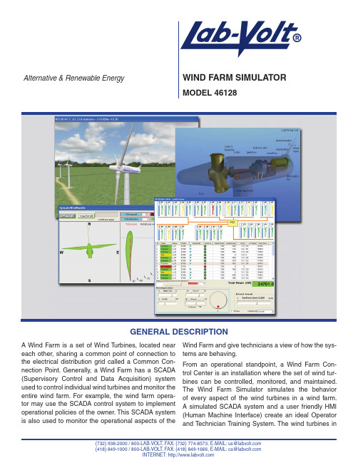
Alternative & Renewable EnergyA Wind Farm is a set of Wind T urbines, located near each other, sharing a common point of connection to the electrical distribution grid called a Common Con-nection Point. Generally, a Wind Farm has a SCADA (Supervisory Control and Data Acquisition) system used to control individual wind turbines and monitor the entire wind farm. For example, the wind farm opera-tor may use the SCADA control system to implement operational policies of the owner. This SCADA system is also used to monitor the operational aspects of the Wind Farm and give technicians a view of how the sys-tems are behaving.From an operational standpoint, a Wind Farm Con-trol Center is an installation where the set of wind tur-bines can be controlled, monitored, and maintained. The Wind Farm Simulator simulates the behavior of every aspect of the wind turbines in a wind farm.A simulated SCADA system and a user friendly HMI (Human Machine Interface) create an ideal Operator and T echnician T raining System. The wind turbines in(732)938-2000/800-LAB-VOLT,FAX:(732)774-8573,E-MAIL:************** (418)849-1000/800-LAB-VOLT,FAX:(418)849-1666,E-MAIL:**************INTERNET: GENERAL DESCRIPTIONWIND FARM SIMULATOR MODEL 46128this software program are modeled after the popular Bonus 1300 K W wind turbine, a variable pitch, stall regulated, dual fi xed speed wind turbine with a squirrel cage asynchronous generator. Additional versions of the Wind Farm Simulator are planned for doubly-fed induction generators.The Wind Farm Simulator is a software-only solution: no special hardware is required, only a PC with ad-equate performance capabilities. The HMI is designed to be user-friendly and intuitive. It presents every pa-rameter as well as the values of the signals, both in-ternal to the wind turbine and published to the SCADA system. Each wind turbine in the wind farm has its own dedicated simulator, enabling users to change indi-vidual parameters independently of the other turbines and observe the resulting behavior of each wind tur-bine. Access to each signal and parameter is designed to easily change the different scenarios that the user may want to create and observe.Controlling and monitoring of the wind turbines is done through communication lines that tie each wind turbine to a central SCADA system where the operator of the Wind Farm can monitor the status and production of each system, shut each system down, give permission for startup, etc. The SCADA system also collects data from the wind turbines and stores it for further analy-sis. All these functionalities are also exercised in the Wind Farm Simulator.The Wind Farm Simulator solves the problem of how to train personnel who must understand the behav-ior of the sub-systems of the wind turbine as well as the wind farm as a whole. Wind farm operators need their technicians to understand hundreds of operating parameters and to be able to react to a plethora of nominal and faulty operating conditions. A technician or operator is able to reproduce with the Wind Farm Simulator situations such as: vibration sensor activat-ed, motor superheated, asymmetry of currents, upper voltage exceeded, lower voltage exceed, (Security) UPS failure, hydraulic brake pump subsystem starting too often or pumping for too long, excessive brake time, gear bearing superheated, thyristors superheated, by-pass contactor welded, bypass contactor not working, excessive angle error in the pitch angle of any of the three blades, pitch oil error, yaw position error, error in the RPM reader, brake lining too thin, gear oil pressure too low, untwisting cables error, etc.Nothing but a wind power generation system simula-tor, operating under an unlimited number of conditions, can impart the type of advanced training required. A simulator is able to create the meteorological as well as electrical, and mechanical operational scenarios that could not be produced on-demand with a real wind turbine.In spite of having access to real systems to train their technical personnel for installing, commissioning and servicing their wind turbines, a simulator is seen as a necessary tool for advanced learning by the wind energy industry.The Wind Farm Simulator addresses these require-ments using two elements within the software: a) elab-orated software models of the behavior of each sub-system in the wind turbine; b) graphic user interfaces that facilitate the setting and visualizing of conditions for these subsystems.TABLE OF CONTENTSGeneral Description (1)T opic Coverage (2)Equipment List (3)Software Description (3)Software Customization ........................................TOPIC COVERAGE• What is a Wind Farm?• What is a Wind Turbine?• Structure of the Wind Farm Simulator• Physics of a Wind Turbine• Wind Farm Operations• Teaching Sessions• Technical Data used in the WFS WT and WFS SCADAGENERAL DESCRIPTION (cont.)2SOFTWARE DESCRIPTIONWind Turbine Block DiagramThe connection of the generator to the grid while in pro-duction is direct. For the “cut-in” operation, the WT uses a set of thyristors for the connection of the generator to the grid during a short, controlled, period of time. The figure above shows the internal structure of a typical WT.Structure of SimulatorThe WFS includes two applications that simulate the behavior of:• an entire wind farm, organized around its SCADA system.• a single wind turbine installed in a wind farmThe WFS’s main purpose is to serve as a training sys-tem for operators of wind farms and service person-nel of industrial wind turbines. The WFS applications follow the principles described below:• Simulators behave as close to their real counterparts as possible.• The Human Machine Interface provides interaction with as many components and subsystems of wind turbines as possible. This complete HMI allows the user to access not only the variables normally avail-able through the Wind T urbine Control T erminal, but also simulated “cables” corresponding to connections among the subsystems. The graphic representations help users identify the wind turbine components.EQUIPMENT LIST FOR WIND FARM SIMULATOR, MODEL 46128QTY DESCRIPTION ORDERING NUMBER 1Binder (87837)3Posters, 11” x 17” (87838)1Wind Farm Simulator Software CD (87422)1Wind Farm Simulator Resource CD (87905)1User Manual ...................................................................................................................................87840-E034WIND FARM SIMULATORMODEL 46128SCADAThe User Interface for the WFS SCADA includes the following items:• Iconic view of each WT , indicating its internal name, its status (Production, Stopped or Out of Order), the actual production (in percent with respect to the maximum), and the cables that connect it to the Point of Common Connection (typically the Substa-tion).• A SCADA view, or a spreadsheet view, where the user can access additional information on each WT and make modifi cations to some of them.• A Maintenance framework through which the user can simulate the change of the WT selected in the SCADA view, from “Out of Order” to “Operational.”• A Production framework, also common in most wind farm SCADAs, where the user can see the actual T otal Power production, together with the Maximum available Power from the wind.• A Meteorological framework where the user can set values for real situations that are obtained from the meteorological station of the Wind Farm.• An “Automatic Dispatching” checkbox through which the user can establish a “manual” of “Automatic Dis-patching” operation of the Wind Farm.• Timing of the evolution of the internal signals are asclose to real counterpart as possible: for example if the blades reported rotational speed is 12 rpms, its 3D representation rotates at that speed.• When convenient, real parameters have been adapt-ed to classroom settings for the sake usability. For example. the angular speed of the yawing in a real turbine is approximately 1º per second, the simulator uses 5º so the changes can happen faster, optimiz-ing the trainee’s time.• These two applications are based on LdP (Lenguaje de Procesos© ACM), a framework specialized for de-veloping and executing simulations.• Both can be executed simultaneously.Synoptics ControlThe Synoptics contain the HMI of the simulator asso-ciated with the confi guration fi le. A synoptic element allows the user to visualize, in real time, the value of specifi ed signals and to modify those values. Shown is the basic control synoptic of the WT Emulator. De-fault view is shown at left; expanded drop-down menu shown at right.5SYNOPTICS USED IN PROGRAM Wind and NacelleThe purpose of the Wind & Nacelle synoptic is:• To allow the user to control wind speed and direction.• To show the Nacelle orientation.• To show the number of cable turns connecting the Nacelle’s generator to the Electric Panel at the bot-tom of the WT .• To show the (simulated) wind vane signal.• To show the signals controlling the yawing motors, the wind vane signal and the power cable turns. There are also control boxes that allow the user to change wind speed and direction, and manually con-trol the yawing motors.Drive TrainThis WTDriveTrain synoptic has been designed to dis-play the most important signals that arrive in the Na-celle emulator, and the signals going out from the Na-celle emulator.The following is a list of these signals:• Rotor speed (rpms), from the Nacelle emulator.• Generator speed (rpms), from the Nacelle emulator.• Pitch value (º), from the Controller emulator.• Hydraulic circuit pressure of the braking system, fromNacelle emulator.• Hydraulic circuit Pump status, from the Controller emulator.• The state of the valve in the hydraulic circuit, con-trolled by the “Soft brake” and “Hard brake” coming from the Controller emulator.• The status of the Pressure switch in the hydraulic cir-cuit.• The Brake Released status (ON or OFF) from the Na-celle emulator.• The state of each Generator connection switch (Large: 4 poles and Small : 6 poles), from the Con-troller emulator.• The state of the Over speed detectors (VCU, HCU)• The state of the T ower vibrations sensor.• The temperatures for the Ambient (setting), Rotor bearing, the Gearbox and the Generator from the Nacelle emulator.It has two main “Views”, selectable through the menu bar: Internal View displays the internal elements in the Nacelle and the Farm View that shows the WT in the Wind Farm.6WIND FARM SIMULATORMODEL 46128Control TerminalElectrical PanelThe multiview Electrical Panel synoptic combines rep-resentations for many aspects of the electrical power circuits of a WT.Each WT is connected to the PCC (Point of Common Connection) on the Wind Farm either in low voltage (typically 690V grid) or at medium voltage (15K V or higher). In the later situation, the WT includes a low-to-medium voltage transformer, generally located in the base of the tower.The various parts of this synoptic display as much information as possible to the user about the param-eters values and a number of internal variables.It is used to display the following information:• Outputs • Inputs• From the Grid • Parameters• Values for internal variables used in the algorithms.• Buttons for the Manual Y awing control • Buttons for activating the “normal” operation (“START”) or passing to Manual control (“STOP”)• Information about the internal State Machines (Op-eration and Security)7Parameters This synoptic is used to see and modify the Param-eters values used in the application. Parameters be-have as output signals or fi xed value generators, eitheranalog or digital.Signals and Connections EditorThis synoptic displays a list of input signals. The colordistinguishes analog or digital signals.Wind Farm Simulator PackageWIND FARM SIMULATORMODEL 46128Refl ecting Lab-Volt’s commitment to high quality standards in product, design, development, production, installation, and service, our manufacturing and distribution facility has received the ISO 9001 certifi cation.Lab-Volt reserves the right to make product improvements at any time and without notice and is not responsible for typographical errors. Lab-Volt recog-nizes all product names used herein as trademarks or registered trademarks of their respective holders. © Lab-Volt 2011. All rights reserved.86906-00 Rev. A8。
windfarm

风能/wind energy空气流动所具有的能量。
风能资源/wind energy resources 大气沿地球表面流动而产生的动能资源。
空气的标准状态/standard atmospheric state 空气的标准状态是指空气压力为101 325Pa,温度为15℃(或绝对288.15K),空气密度1.225kg/m 3 时的空气状态。
风速/wind speed 空间特定点的风速为该点空气在单位时间内所流过的距离。
平均风速/average wind speed 给定时间内瞬时风速的平均值。
年平均风速/annual average wind speed 时间间隔为一整年的瞬时风速的平均值。
最大风速/maximum wind speed 10分钟平均风速的最大值。
极大风速/extreme wind speed 瞬时风速的最大值。
阵风/gust 超过平均风速的突然和短暂的风速变化。
年际变化/inter-annual variation 以30年为基数发生的变化。
风速年际变化是从第1年到第30年的年平均风速变化。
[风速或风功率密度]年变化/annual variation 以年为基数发生的变化。
风速(或风功率变化)年变化是从1月到12月的月平均风速(或风功率密度)变化。
[风速或风功率密度]日变化/diurnal variation 以日为基数发生的变化。
月或年的风速(或风功率密度)日变化是求出一个月或一年内,每日同一钟点风速(或风功率密度)的月平均值或年平均值,得到0点到23点的风速(或风功率密度)变化。
风切变/wind shear 风速在垂直于风向平面内的变化。
风切变指数/wind shear exponent 用于描述风速剖面线形状的幂定律指数。
风速廓线/wind speed profile, wind shear law 又称“风切变律”,风速随离地面高度变化的数学表达式。
湍流强度/turbulence intensity 标准风速偏差与平均风速的比率。
大型风机偏航状态力学分析及偏航控制策略研究

大型风机偏航状态力学分析及偏航控制策略研究卢晓光;岳红轩;吴鹏;刘伟鹏;李凤格【摘要】为制定合理的偏航控制策略,研究了偏航状态下叶片吸收风能的特性,分析了偏航状态下的叶片受力特性,并研究了偏航误差在不同风速下对风轮空气动力的影响;根据偏航状态受力分析,制定了分风速段变参数偏航控制策略,讨论了策略实现中关键数据处理方式.经风场测试表明,此策略完全能满足风机对偏航的要求,经仿真数据的外推法统计分析,此策略能在不影响整机受力及发电量的情况下,减少寿命周期内的偏航次数,提高偏航机构寿命.【期刊名称】《可再生能源》【年(卷),期】2014(032)007【总页数】5页(P973-977)【关键词】受力分析;偏航控制;数据处理;滤波;bladed仿真【作者】卢晓光;岳红轩;吴鹏;刘伟鹏;李凤格【作者单位】许昌许继风电科技有限公司,河南许昌461000;许昌许继风电科技有限公司,河南许昌461000;许昌许继风电科技有限公司,河南许昌461000;许昌许继风电科技有限公司,河南许昌461000;许昌许继德理施尔电气有限公司,河南许昌461000【正文语种】中文【中图分类】TM6140 引言风力发电机控制器的开发需要力学、控制理论、数据处理技术等多学科知识综合应用1],[2],片面强调控制算法的复杂度及控制精度,不仅不能达到最优控制的效果[3],反而会造成相关部件寿命的缩短和不确定性故障的增加。
制定风机偏航控制策略,要从偏航动作特性及整机对偏航的要求出发,研究偏航状态下的整机力学特性[4],[5],从而指导偏航策略的制定,以达到风机运行中各种制约因素之间的平衡[6]。
本文首先从偏航状态下的叶片气动受力出发,分析动量定理及Glauert动量定理在偏航状态下的应用,并在此基础上分析了偏航误差随风速变化导致叶片受力及偏航力矩的变化情况。
然后以偏航状态风轮受力及风轮吸收功率特性为指导,制定了相关的偏航控制策略。
最后分析了实现上述策略的关系数据处理方法。
- 1、下载文档前请自行甄别文档内容的完整性,平台不提供额外的编辑、内容补充、找答案等附加服务。
- 2、"仅部分预览"的文档,不可在线预览部分如存在完整性等问题,可反馈申请退款(可完整预览的文档不适用该条件!)。
- 3、如文档侵犯您的权益,请联系客服反馈,我们会尽快为您处理(人工客服工作时间:9:00-18:30)。
Generic Aggregated Wind Farm Model for Power System Simulations – Impact of Grid Connection RequirementsJ. Soens, J. Driesen, D. Van Hertem, R. BelmansDepartment of Electrical EngineeringESAT/ELECTA, K.U.LeuvenKasteelpark Arenberg 10, B-3001 Leuven (Belgium)phone: +32 16 321031, fax: +32 16 321985e-mail: joris.soens@esat.kuleuven.ac.beAbstractA generic dynamic model of a large wind farm is used to simulate the grid impact of an offshore wind farm in Belgium. The voltage fluctuations during wind speed changes and grid disturbances are simulated. The outcome depends on the performance of the dynamic voltage support that the wind farm can deliver.KeywordsPower system simulation, Wind power generation, Wind power modelling1.IntroductionThe steadily increasing amount of wind power throughout various UCTE-countries puts new challenges to the power system operators, who have to ensure a reliable, safe and economically manageable grid operation. Therefore, the modelling of wind turbines for power system simulations is a matter of high interest. The development of these models has been the subject of many discussions: it requires a compromise between making substantial simplifications to reduce computational efforts on the one hand, and maintaining the necessary adequacy to be able to predict the farm’s influence on the system’s dynamic behaviour on the other hand.With adequate dynamic models, more insight is obtained about the ability of a wind farm to provide ‘grid support’. ‘Grid support’, also known as ‘ancillary services’, represents a number of services that the power system operator requires from power generators, in order to secure a safe, reliable, stable and economically manageable grid operation. These ‘ancillary services’ include support for:- (fast) output power or frequency control;- voltage control;- black start capability;- economic dispatch and financial trade reinforcementsThe relation between wind farms and grid support has been extensively discussed over the past years, especially in Denmark and Germany, where the relative amount of wind power in the power grid is the highest of Europe. Specific grid connection requirements for wind turbines were issued first by the Danish and German grid operators, and are used as a reference by most European grid operators who have to take a large amount of wind power in their power system into account. An overview of existing grid connection requirements is given in [2] (specific for wind turbines) and [3] (dispersed generation in general).The actual existing grid connection requirements are mainly focussed on the first two mentioned ancillary services: (fast) output power control and voltage control. For these issues, the advanced wind turbine generators can be considered as competent as conventional generators.On the other hand, even the most advanced turbine technology does hardly improve the capability of wind power to facilitate the economic dispatch of the power market and financial trade reinforcements. These issues can not be enforced by technical grid connection requirements, but must be part of the economical risk that a wind farm operator is willing to take. The criterion for success in these issues is mainly the accuracy of wind speed predictions on a (mid-)long term, rather than the turbine technology. This will not be further discussed in this paper.In this paper, the importance of a wind farm’s capability to provide voltage control is examined. As an example study case, simulations are performed for a hypothetical offshore wind-farm in the Belgian North-Sea. A simplified generic model is used for the wind farm. This model is fully described in [4] and is only shortly reviewed in the next section. The used power system simulation software is EUROSTAG.This work is part of the multidisciplinary research project ‘Optimal Offshore Wind Development in Belgium’, funded by the Belgian Federal Science Office. The project takes meteorological, geological, technological and economical aspects of offshore wind power in Belgium into account, as well as the grid availability. Thestatic load-flow results for the grid availability have already been published in [5]. It was concluded there that an installed offshore wind power of more than 500MW in Belgium will require major grid reinforcements both in the coast region and further inland, which is not expected to happen in the near future, considering the difficulties in obtaining permits for constructing new power lines.2. Wind Farm ModelA. Generic Active Power ModelA full description of the generic wind farm model can be found in [4]. The active power model starts from a detailed model of a variable speed turbine, published by the manufacturer [6]. This model was used to perform simulations with sinusoidal wind speeds with a varying average value and varying fluctuation frequency (Fig. 1). All simulation results are summarized in the plot of Fig. 2, in which the amplitude of the power oscillations is plotted against the fluctuation frequency of the wind speed, using the average wind speed as parameter.Two sets of curves can be distinguished: curves for high average wind speed (slope 20dB/decade in low frequency region) and for low average wind speed (horizontal in low frequency region). The reason for this is the different effect of speed and pitch control of the turbine, below and above rated wind speed.vw i n d /v w i n d ,r,Pm e c h/Pm e c h ,rvw i n d /v w i n d ,r, Pm e c h/Pm e c h ,rtime [s]time [s]time [s]d)Fig. 1. Wind speed and mechanical power for two values of average wind speed and three different wind speedfluctuation frequenciesPamplitude-frequency characteristicvwindfluctuation frequency [rad/s]f l u c t u a t i ng Pm e c h , a m p l i t u d e [d B ]Fig. 2. Frequency Characteristic of Power FluctuationAmplitudeThe curves of Fig. 2 suggest to simplify the detailedactive power model by two equivalent transfer functions, one for high and one for low wind speeds (Fig. 3). The time constants are calculated to have an optimal match between the curves of and the frequency response of the transfer functions. Suggested values are:T low = 7 s d = 0.3 T 0 = 0.5 s K high = 0.06available windspeed v wind,a v a i ltransfer function for low wind speedgradual transition low wind speed -> high wind speedpower curveadditional transfer functionf o r h igh wi n d s p e e dlow-p a s s filter1Fig. 3. Equivalent Transfer Function forActive PowerThus, an equivalent active power model for a wind turbine is constructed, which is well suitable to estimate the turbine power fluctuations during continuous operation. The full explanation of the model derivation, as well as the aggregation into a model of an entire wind farm, is given in [4]. Also the simplified simulation of turbine yawing and active power control is given in [4].B. Generic Reactive Power ModelThe modelling of the reactive power generation and the behaviour during grid disturbances does not start from a predefined detailed model from literature. It is believed that future large wind farms will always be able to control the reactive power output, either by control action on the generator itself or by additional devices (such as SVCs or STATCOMs) connected at the point of common coupling.The supplied reactive power is calculated by either a P-controller or PI-controller with anti-windup, to avoid that the reference reactive power exceeds a l imit value. The implementation of a PI-controller is supported by most power system simulation software packages, and does not contain any particularities in its use for this model.The speed of the reactive current control depends on the generator type. T he two most common generator types for variable speed turbines are- doubly fed induction generators- synchronous generators with frequencyconverter, (mostly combined with a ‘direct drive’ turbine configuration)The current control loop for the reactive power is modelled as a first order delay (from reference current towards produced current). The current control loop of the synchronous generator is much faster than with the doubly fed induction generator, as the full active and reactive power is processed by power electronic converters. Suggested values for the time constant TICTL (the time constant of the current control loop) are:- TICTL = 2 s for poorly advanced technology-TICTL = 200 ms for advanced technology(doubly fed induction generator)-TICTL = 20 ms for highly advancedtechnology (synchronous generatorwith PWM-converter, or a STATCOMconnected parallel with the farm)A detailed description about the modelling of the current controller, as well as the impact of the reactive current control on the active power control (in case of overcurrents) can be found in [4]. It is assumed that the reactive power has priority on the active power, i.e. in case of reactive power demand and high machine currents, the active power must be decreased in order to supply the reactive power, without exceeding the rated currents.3.SimulationsA.Assumptions for Simulated ScenariosWind FarmThe wind farm is assumed to consist of five turbine rows behind each other, orthogonal to the wind speed direction. The wind farm installed power is 500MW.Grid ConnectionThe grid connection is shown in Fig. 4. The wind farm power is assumed to be collected at 30kV, and transformed by an offshore transformer towards 150kV. The grid connection is made by a submarine 150kV cable. There are three 150kV-substations available at the Belgian coast (Slijkens, Zeebrugge and Koksijde). The wind farm is assumed to be connected at Slijkens.The cable characteristics have impact on the simulation results, especially its capacitance is not neglectible, As the cable consumes a lot of capacitive power, two inductors are assumed, each of them compensating half of the cable capacitive power in no-load condition. One is installed at Slijkens, the other at the 150kV offshore substation. The inductors are not controlled and do not have an impact on the dynamic simulations.Belgian Power System ModelAn Eurostag model of the Belgian power grid was used, containing:-all 400 kV, 220kV 150kV and 70kV substations and high voltage lines of Belgium, including theplanned 150kV cable between the coastal nodesKoksijde and Slijkens;-all generation and load data for each substation, as they have been recorded on a representativewinter day (19/01/1994);-dynamic models of the governors and voltage controllers of most generators in the Belgianpower system, including the power plant ofHerdersbrug (2 x 144MW and 1 x 165 MW),which is the nearest power plant to the coast.Model of Belgian GridFig. 4. Connection of Wind Farm to Belgian GridB.Wind Speed ChangesThe impact of wind speed changes on the voltage on the grid node at which the farm is connected is investigated. Four scenarios are considered:a) the wind farm is controlled to produce nor consume reactive power at the offshore 150kV-node; the transmission cable length is 10 kmb) same as a), but with a cable length of 50km;c) the wind farm reactive power is dynamically controlled in such a way that the voltage at Slijkens remains at a fixed value (i.e. the initial voltage without wind power production). The transmission cable length is 10km;d) same as c), but with a cable length of 50km.A wind speed sequence as in Fig. 5 is assumed. Starting from 10m/s, the wind speed rises at 14m/s (i.e. the turbine rated wind speed), and then further to 25 m/s (i.e. just below the cut-out wind speed). The wind speed direction undergoes a sudden change of 28 degrees (0.5 radians) at t = 5000s. The turbines must yaw towards the new wind direction. The mismatch angle between the wind direction and the turbines orientation, calculated according to the model description in [4] is also shown in Fig. 5.The active power production is shown in Fig. 6. The moments at which the wind gust (at t = 1000 s) reaches each of the five turbine rows can be clearly distinguished.A sudden wind speed increase results in a power increase towards rated power in approximately 150 s. The farm rated power is not fully achieved because of the farm losses, causing a reduction of wind speed for the turbines behind the first row. The rated power is achieved when the wind speed increases further to 25 m/s. The turbines then have to pitch the blades out of the wind in order to avoid excessive mechanical loads on the turbine or excessive power production. The pitching action goes rather fast, and the farm is able to maintain its output power within a narrow range around its rated power. Themoments at which the wind speed gust reaches each of the five turbine rows is again clearly noticeable. The change in wind speed direction (t = 5000s) also causes a short drop in power production, which is quickly restored by the yawing action of the turbines.For the active power production, no differences were noted between the four scenarios a, b, c or d.The produced reactive power for each of the four scenarios is shown in Fig. 7. It is zero for cases a and b by definition, and is permanently adapted in cases c and d to provide voltage control.A wind farm that performs dynamic voltage control has to deliver more reactive power for a 10km -cable (case c) then for a 50km cable (case d). The long capacitive cable damps voltage oscillations and supplies part of the required reactive power.The resulting voltage in Slijkens and at the offshore 150kV – substation are shown in Fig. 8 and in Fig. 9. Without voltage control, the voltage at Slijkens fluctuates with changing wind speed. In the cases with voltage control, the voltage can well be maintained at a fixed value. However, the voltage fluctuations at Slijkens for the cases a and b are far less than 1%, and thus well within the normal voltage fluctuations that appear on a power system. A wind farm operation strategy at which the farm reactive power is controlled at a fixed value does not result in a gravely decreased grid power quality.All scenarios were investigated considering the three values for the current control speed TICTL (20 ms, 200 ms, 2 s). However, the differences for different TICTL -values were hardly visible. The active power oscillations are very slow, due to the acceleration and deceleration of the generators in case of wind speed changes. Therefore, the advantages of a highly advanced generator control system are not relevant in this matter.time [s]w i n d s p e e d [m /s ] a n d d i r e c t i o n [d e g ]Fig. 5. Assumed Wind Speed and Wind direction for WindGust Simulationtime [s]f a r m p o w e r[M W ]time [s]time [s]Fig. 6. Active Power Production by a 500MW -Wind Farmtime [s]f a r m r e a c t i v e p o w e r [M V A r ]time [s]time [s]Fig. 7. Reactive Power Production by a 500MW -WindFarmtime [s]VS l i j k e n s[k V ]time [s]time [s]Fig. 8. Voltage at Slijkens 150kV-substationtime [s]V S l i j k e n s [k V ]time [s]time [s]Fig. 9. Voltage at offshore 150kV-nodeAs a conclusion, during normal wind farm operationthere is no incentive to set up severe grid connection requirements that demand dynamic voltage control from the wind farm. It is well sufficient to demand a controllable and fixed power factor, close to 100%. However, during voltage disturbances, there will be need for dynamic voltage support, as will be discussed in the next paragraph.C.Voltage Disturbance due to Grid FaultA short-circuit at one of the two parallel lines from Slijkens to Brugge (see Fig. 4) is simulated. This causes a voltage dip at the surrounding nodes. The short-circuit lasts 0.5s, and it is assumed that no lines are tripped. The voltage at Slijkens during the grid fault depends on the reactive power support of the wind farm.For the following simulation example, the wind farm is assumed to be connected as in Fig. 4, with a 150 kV - submarine cable of 10 km. The wind speed is 13 m/s (resulting in an active power production of 355MW) and does not change during the grid disturbance.Four scenarios for the reactive power control (Dynamic VAr control or ‘DVAr’) are considered:-no DVAr, reactive power permanently controlled at zero;-slow DVAr (T ICTL = 2 s), corresponding with poorly advanced technology-fast DVAr (TICTL = 200 ms), corresponding with advanced technology-ultra-fast DVAr (TICTL = 20 ms), corresponding with higly advanced technologyThe current limits are set as follows:-the maximum reference reactive current is 100% of the rated current. Reactive current control haspriority on active current in case of voltage dips,as is demanded in most grid connectionrequirements;-when the total current exceeds its rated value, the active power of the farm is decreased, using pitchcontrol. The time constant for the pitch controller(as explained in [4]) is 4 s.The voltage at Slijkens for these four cases is shown in Fig. 10. The voltage cannot be fully restored, because the required reactive power exceeds the farm’s current limits. The voltage for the fastest DVAr-control case first increases shortly after the grid fault (due to the supplied reactive current), and then decreases again after approximately 100 milliseconds. The reason for this is the decrease of active power production, in order to prevent long-lasting overcurrents. After the fault clearance, the voltage jumps to a very high value in the cases with DVAr-control, because of the high amount of reactive current delivered. The voltage is however quickly controlled towards its original value. For the cases without or with very slow DVAr-control, the voltage keeps fluctuating after the fault clearance. This is due to the influence of the various voltage controllers further in the grid (e.g. the Herdersbrug power plant). The wind farm’s active, reactive and total current for each of the four scenarios is shown in Fig. 11. The active power is shown in Fig. 12. Fast reactive power support requires also fast active power decrease, in order to limit the current.time [s]VoltageatSlijkens[kV]Fig. 10. Voltage at Slijkens during Grid Disturbance, forfour DVAr-scenariostime [s]farmcurrent[%ofrated]time [s]no DVAr DVAr, TICTL = 2 sDVAr, TICTL = 200 ms DVAr, TICTL = 20 ms Fig. 11. Total, Active and Reactive Current of the WindFarm during Grid Disturbance, for four DVAr-scenariostime [s]farmpower[MW]Fig. 12. Wind Farm Active Power during Grid Disturbance,for four DVAr-scenarios4.ConclusionsA generic dynamic wind farm model has been constructed, in order to assess the impact of a possible offshore wind farm on the Belgian high voltage grid. The model is used to evaluate the influence of the wind farm’s dynamic VAr control on the grid voltage.It must be noted that many parts of the model are not specific to wind turbines, but generally applicable for various kinds of generators and loads that are connected to the grid through power electronic interfaces.For wind speed fluctuations during normal operation, the difference between dynamic VAr control and simply operating at a fixed power factor is hardly visible for a 500MW-wind farm. It is thus a sufficient grid connection requirement towards wind farms to demand a power factor within a narrow range of 100%, as long as no grid disturbances occur, and the installed power remains limited. However, depending on the amount of installed offshore wind power foreseen in the future, the grid operator may decide to set up demands for voltage control from the beginning. This way, the wind farms that will be built after the first one are treated fairly. Voltage control during normal grid operation is advised when more than approximately 1000MW offshore wind power is installed. This high installed power would however require major grid reinforcements to prevent line overloads [5]. In the Belgian case, the power rating of the high voltage lines puts a more severe limit to the maximum amount of installed wind power than the impact on the grid voltage.In the case of a voltage dip due to a grid disturbance further inland, fast Dynamic VAr support by the wind farm can alleviate considerably the voltage disturbance at the point of common coupling. The alleviation of the voltage dip can save the wind farm from be tripped of the grid by its voltage protection relays. However, precautions must be made to ensure that the active power can be decreased sufficiently fast. This way, long lasting overcurrents are avoided when the full current capacity is used for reactive power support. AcknowledgementThis research is part of the research project Optimal Offshore Wind Energy Developments in Belgium, promoted by the Belgian Federal Science Office and the IWT-GBOU project ‘Embedded Generation: A Global Approach To Energy Balance And Grid Power Quality And Security’.The authors are also grateful to the Belgian ‘Fonds voor Wetenschappelijk Onderzoek (F.W.O.) - Vlaanderen’ for their financial support of this work. J. Soens is a doctoral research assistant of the F.W.O.-Vlaanderen. J. Driesen holds a postdoctoral research fellowship of the F.W.O.- Vlaanderen”.References[1]S. Stoft, ‘Power System Economics’, John Wiley &Sons; 1st edition (May 17, 2002);[2]S.M. Bolik, ‘Grid Requirements Challenges forWind Turbines’, 4th International Workshop on Large-Scale Integration of Wind Power and Transmission Networks of Offshore Wind Farms, 20-21 October, Billund, Denmark;[3]Dussart, M.; Lauwers, P.; Magnus, S.; Laperches,Y.; ‘Connection requirements for dispersed generation: evolutions of existing requirements and need for further standardization’, CIRED. 16th International Conference and Exhibition on Electricity Distribution (IEE Conf. Publ No. 482) , Volume: 4 , 18-21 June 2001;[4]J. Soens, J. Driesen, R. Belmans, ‘Generic DynamicWind Farm Model for Power System Simulations,’ Nordic Wind Power Conference NWPC’04, Chalmers University of Technology, Göteborg, Sweden, 1-2 March 2004;[5]Van Roy P., Soens J., Driesen J., Belmans R.,‘Impact of off-shore wind power on the Belgian HV-grid,’ European wind energy conference EWEC, June 16-19, 2003, Madrid, Spain;[6]R. W. Delmerico, N. Miller, W. W. Price, J. J.Sanchez-Gasca, ‘Dynamic Modelling of GE 1.5 and3.6 MW Wind Turbine-Generators for StabilitySimulations,’ IEEE Power Engineering Society PES General Meeting, 13-17 July, Toronto, Canada;。