A 2-D graphical representation of protein sequences based on nucleotide triplet codons[

合集下载

Review article Linear optical quantum computing

a r X i v :q u a n t -p h /0512071v 2 14 M a r 2006Linear optical quantum computingPieter Kok,1,2,∗W.J.Munro,2Kae Nemoto,3T.C.Ralph,4Jonathan P.Dowling,5,6and burn 41Department of Materials,Oxford University,Oxford OX13PH,UK2Hewlett-Packard Laboratories,Filton Road Stoke Giﬀord,Bristol BS348QZ,UK3National Institute of Informatics,2-1-2Hitotsubashi,Chiyoda-ku,Tokyo 101-8430,Japan 4Centre for Quantum Computer Technology,University of Queensland,St.Lucia,Queensland4072,Australia5Hearne Institute for Theoretical Physics,Department of Physics and Astronomy,LSU,Baton Rouge LA,70803,USA6Institute for Quantum Studies,Department of Physics,Texas A&M University,77843-4242,USA(Dated:February 1,2008)Linear optics with photon counting is a prominent candidate for practical quantum computing.The protocol by Knill,Laﬂamme,and Milburn [Nature 409,46(2001)]explicitly demonstrates that efﬁcient scalable quantum computing with single photons,linear optical elements,and projective measure-ments is possible.Subsequently,several improvements on this protocol have started to bridge the gap between theoretical scalability and practical implementation.We review the original theory and its improvements,and we give a few examples of experimental two-qubit gates.We discuss the use of realistic components,the errors they induce in the computation,and how these errors can be corrected.PACS numbers:03.67.Hk,03.65.Ta,03.65.UdContentsI.Quantum computing with light 1A.Linear quantum optics2B.N port interferometers and optical circuits 4C.Qubits in linear optics4D.Early optical quantum computers and nonlinearities 6II.A new paradigm for optical quantum computing8A.Elementary gates8B.Parity gates and entangled ancillæ10C.Experimental demonstrations of gates 11D.Characterisation of linear optics gates 13E.General probabilistic nonlinear gates14F.Scalable optical circuits and quantum teleportation 15G.The Knill-Laﬂamme-Milburn protocol 16H.Error correction of the probabilistic gates 18III.Improvements on the KLM protocol19A.Cluster states in optical quantum computing 19B.The Yoran-Reznik protocol 21C.The Nielsen protocol22D.The Browne-Rudolph protocol22E.Circuit-based optical quantum computing revisited 24IV .Realistic optical components and their errors25A.Photon detectors 25B.Photon sources27C.Circuit errors and quantum memories 32V .General error correction33A.Correcting for photon loss33B.General error correction in LOQC 35VI.Outlook:beyond linear optics36Acknowledgements 37References382The difﬁculty with this technique is that such optical quantum gates are probabilistic:More often than not, the gate fails and destroys the information in the quan-tum computation.This can be circumvented by using an exponential number of optical modes,but this is by deﬁnition not scalable(see also section I.D).In2001, Knill,Laﬂamme,and Milburn(KLM2001)constructed a protocol in which probabilistic two-photon gates are teleported into a quantum circuit with high probabil-ity.Subsequent error correction in the quantum circuit is used to bring the error rate down to fault-tolerant levels. We describe the KLM protocol in detail in section II. Initially,the KLM protocol was designed as a proof that linear optics and projective measurements allow for scalable quantum computing in principle.However, it subsequently spurred on new experiments in quan-tum optics,demonstrating the operation of high-ﬁdelity probabilistic two-photon gates.On the theoretical front, several improvements of the protocol were proposed, leading to ever smaller overhead cost on the computa-tion.A number of these improvements are based on cluster-state quantum computing,or the one-way quan-tum computer.Recently,a circuit-based model was shown to have similar scaling properties as the best-known cluster state model.In section III,we describe the several improvements to linear optical quantum in-formation processing in considerable detail,and in sec-tion IV,we describe the issues involved in the use of realistic components such as photon detectors,photon sources and quantum memories.Given these realistic components,we discuss loss tolerance and general er-ror correction for Linear Optical Quantum Computing (LOQC)in section V.We will restrict our discussion to the theory of single-photon implementations of quantum information pro-cessors,and we assume some familiarity with the ba-sic concepts of quantum computing.For an introduc-tion to quantum computation and quantum informa-tion,see e.g.,Nielsen and Chuang(2000).For a re-view article on optical quantum information process-ing with continuous variables,see Braunstein and Van Loock(2005).In section VI we conclude with an outlook on other promising optical quantum informa-tion processing techniques,such as photonic band-gap structures,weak cross-Kerr nonlinearities,and hybrid matter-photon systems.We start our review with a short introduction to linear optics,N port optical interferome-ters and circuits,and we deﬁne the different versions of the optical qubit.A.Linear quantum opticsThe basic building blocks of linear optics are beam split-ters,half-and quarter-wave plates,phase shifters,etc. In this section we will describe these devices mathemat-ically and establish the convention that is used through-out the rest of thepaper.n|n−1 andˆa†|n =√Physically,a phase shifter is a slab of transparent mate-rial with an index of refraction that is different from thatof free space.Another important component is the beam splitter(see Fig.1).Physically,it consists of a semi-reﬂective mir-ror:when light falls on this mirror,part will be reﬂected and part will be transmitted.The theory of the lossless beam splitter is central to LOQC,and was developed by Zeilinger(1981)and Fearn and Loudon(1987).Lossybeam splitters were studied by Barnett et al.(1989).The transmission and reﬂection properties of general dielec-tric media were studied by Dowling(1998).Let the two incoming modes on either side of the beam splitter be denoted byˆa in andˆb in,and the outgoing modes byˆa out andˆb out.When we parameterise the probability ampli-tudes of these possibilities as cosθand sinθ,and the relative phase asϕ,then the beam splitter yields an evo-lution in operator formˆa†out=cosθˆa†in+ie−iϕsinθˆb†in,ˆb†=ie iϕsinθˆa†in+cosθˆb†in,(4) outThe reﬂection and transmission coefﬁcients R and T of the beam splitter are R=sin2θand T=1−R=cos2θ. The relative phase shift ie±iϕensures that the transfor-mation is unitary.Typically,we choose eitherϕ=0or ϕ=π/2.Mathematically,the two parametersθandϕrepresent the angles of a rotation about two orthogonal axes in the Poincar´e sphere.The physical beam splitter can be described by any choice ofθandϕ,provided the correct phase shifts are applied to the outgoing modes. In general the Hamiltonian H BS of the beam splitter evolution in Eq.(4)is given byH BS=θe iϕˆa†inˆb in+θe−iϕˆa inˆb†in.(5) Since the operator H BS commutes with the total number operator,[H BS,ˆn]=0,the photon number is conserved in the lossless beam splitter,as one would expect.The same mathematical description applies to the evolution due to a polarisation rotation,physically im-plemented by quarter-and half-wave plates.Instead of having two different spatial modes a in and b in,the two incoming modes have different polarisations.We write ˆa in→ˆa x andˆb in→ˆa y for some orthogonal set of coor-dinates x and y(i.e., x|y =0).The parametersθandϕare now angles of rotation:ˆa†x′=cosθˆa†x+ie−iϕsinθˆa†y,ˆa†y′=ie iϕsinθˆa†x+cosθˆa†y.(6) This evolution has the same Hamiltonian as the beam splitter,and it formalises the equivalence between the so-called polarisation and dual-rail logic.These trans-formations are sufﬁcient to implement any photonic single-qubit operation(Simon and Mukunda1990). The last linear optical element that we highlight here is the polarising beam splitter(PBS).In circuit diagrams,5of choice is usually taken to be a single photon that has the choice of two different modes|0 L=|1 ⊗|0 ≡|1,0 and|1 L=|0 ⊗|1 ≡|0,1 .This is calleda dual-rail qubit.When the two modes represent the internal polarisation degree of freedom of the photon (|0 L=|H and|1 L=|V ),we speak of a polari-sation qubit.In this review we will reserve the term “dual rail”for a qubit with two spatial modes.As we showed earlier,these two representations are mathe-matically equivalent,and we can physically switch be-tween them using polarisation beam splitters.In addi-tion,some practical applications(typically involving a dephasing channel such as aﬁbre)may call for so-called time-bin qubits,in which the two computational qubit values are“early”and“late”arrival times in a detec-tor.However,this degree of freedom does not exhibit a natural internal SU(2)symmetry:Arbitrary single-qubit operations are very difﬁcult to implement.In this review we will be concerned mainly with polarisation and dual-rail qubits.In order to build a quantum computer,we need both single-qubit operations as well as two-qubit operations. Single-qubit operations are generated by the Pauli op-eratorsσx,σy,andσz,in the sense that the operator exp(iθσj)is a rotation about the j-axis in the Bloch sphere with angleθ.As we have seen,these operations can be implemented with phase shifters,beam splitters, and polarisation rotations on polarisation and dual-rail qubits.In this review,we will use the convention that σx,σy,andσz denote physical processes,while we use X,Y,and Z for the corresponding logical operations on the qubit.These two representations become inequiva-lent when we deal with logical qubits that are encoded in multiple physical qubits.Whereas single-qubit operations are straightforward in the polarisation and dual-rail representation,the two-qubit gates are more problematic.Consider,for exam-ple,the transformation from a state in the computational basis to a maximally entangled Bell state:|H,H ab→12(|H,V cd+|V,H cd).(13)This is the type of transformation that requires a two-qubit gate.In terms of the creation operators(and ig-noring normalisation),the linear optical circuit that is supposed to create Bell states out of computational ba-sis states is described by a Bogoliubov transformation of both creation operatorsˆa†Hˆb†H→ ∑k=H,Vαkˆc†k+βkˆd†k ∑k=H,Vγkˆc†k+δkˆd†k =ˆc†Hˆd†V+ˆc†Vˆd†H.(14)It is immediately clear that the right-hand sides in both lines cannot be made the same for any choice ofαk,βk,γk,andδk:The top line is a separable expression in the creation operators,while the bottom line is an entangled expression in the creation operators.Therefore,linear optics alone cannot create maximal polarisation entan-glement from single polarised photons in a determinis-tic manner(Kok and Braunstein2000a).Entanglement that is generated by changing the deﬁnition of our sub-systems in terms of the globalﬁeld modes is inequiv-alent to the entanglement that is generated by apply-ing true two-qubit gates to single-photon polarisation or dual-rail qubits.Note also that if we choose our representation of the qubit differently,we can implement a two-qubit transformation.Consider the single-rail qubit encoding |0 L=|0 and|1 L=|1 .That is,the qubit is given by the vacuum and the single-photon state.We can then implement the following(unnormalised)transfor-mation deterministically:|1,0 →|1,0 +|0,1 .(15) This is a50:50beam splitter transformation.However, in this representation the single-qubit operations cannot be implemented deterministically with linear optical el-ements,since these transformations do not preserve the photon number(Paris2000).This implies that we can-not implement single-qubit and two-qubit gates deter-ministically for the same physical representation.For linear optical quantum computing,we typically need the ability to(dis-)entangleﬁeld modes.We therefore have to add a non-linear component to our scheme.Two possible approaches are the use of Kerr nonlinearities, which we brieﬂy review in the next section,and the use of projective measurements.In the rest of this review,we concentrate mainly on linear optical quantum comput-ing with projective measurements,based on the work by Knill,Laﬂamme,and Milburn.Finally,in order to make a quantum computer with light that can outperform any classical computer,we need to understand more about the criteria that make quantum computers“quantum”.For example,some simple schemes in quantum communication require only superpositions of quantum states to distinguish them from their corresponding classical ones.However, we know that this is not sufﬁcient for general computa-tional tasks.First,we give two deﬁnitions.The Pauli group P is the set of Pauli operators with coefﬁcients {±1,±i}.For instance,the Pauli group for one qubit is{11,±X,±Y,±Z,±i11±iX,±iY,±iZ,}where11is the identity matrix.The Pauli group for n qubits consists of elements that are products of n Pauli operators,in-cluding the identity.In addition,we deﬁne the Clifford group C of transformations that leave the Pauli group in-variant.In other words,for any element of the Clifford group c and any element of the Pauli group p,we havecpc†=p′with p′∈P.(16) Prominent members of the Clifford group are the Hadamard transformation,phase transformations,and8can be achieved with a single two-level atom in a one-sided cavity.The cavity effectively enhances the tiny nonlinearity of the atom.The losses in this system are negligible.In sectionVI we will return to systems in which (small)phase shiftscanbe generated using nonlinear optical interactions,but the principal subject of this re-view is how projective measurements can induce enough of a nonlinearity to make linear optical quantum com-puting possible.II.A NEW PARADIGM FOR OPTICAL QUANTUM COMPUTINGIn 2000,Knill,Laﬂamme,and Milburn proved that it is indeed possible to create universal quantum computers with linear optics,single photons,and photon detection (Knill et al.2001).They constructed an explicit protocol,involving off-line resources,quantum teleportation,and error correction.In this section,we will describe this new paradigm,which has become known as the KLM scheme ,starting from the description of linear optics that we developed in the previous section.In sections II.A,II.B and II.C,we introduce some elementary probabilis-tic gates and their experimental realizations,followed by a characterisation of gates in section II.D,and a gen-eral discussion on nonlinear unitary gates with projec-tive measurements in section II.E.We then describe how to teleport these gates into an optical computational cir-cuit in sections II.F and II.G,and the necessary error correction is outlined in section II.H.Recently,Myers and Laﬂamme (2005)published a tutorial on the origi-nal “KLM theory.”A.Elementary gatesPhysically,the reason why we cannot construct deter-ministic two-qubit gates in the polarisation and dual-rail representation,is that photons do not interact with each other.The only way in which photons can directly in-ﬂuence each other is via the bosonic symmetry relation.Indeed,linear optical quantum computing exploits ex-actly this property,i.e.,the bosonic commutation rela-tion [ˆa,ˆa †]=1.To see what we mean by this statement,consider two photons in separate spatial modes inter-acting on a 50:50beam splitter.The transformation will be|1,1 ab =ˆa †ˆb †|0 →12ˆc †2−ˆd †2 |0 cd =12(|2,0 cd −|0,2 cd ).(22)It is clear (from the second and third line)that the bosonic nature of the electromagnetic ﬁeld gives rise toCZ |0 |0,0|1 |0,1 |1|1,0|1 |1,0(24)which is identical to|q 1,q 2 →CZ (−1)q 1q 2|q 1,q 2 (25a)|q 1,q 2→CNOT|q 1,q 2⊕q 1 .(25b)FIG.7The nonlinear sign (NS)gate according to Knill,Laﬂamme and Milburn.The beam splitter transmission am-plitudes are η1=η3=1/(4−2√2.2,then the output state isa maximally entangled state.The overall probability of this CZ gate p CZ =p 2NS .It is immediately clear that we cannot make the NS gate with a regular phase shifter,because only the state |2 picks up a phase.A linear optical phase shifter would also induce a factor i (or −i )in the state |1 .How-ever,it is possible to perform the NS-gate probabilistically using projective measurements.The fact that two NS gates can be used to create a CZ gate was ﬁrst realized by Knill,Laﬂamme,and Milburn (2001).Their proba-bilistic NS gate is a 3-port device,including two ancil-lary modes the output of which is measured with perfect photon-number discriminating detectors (see Fig.7).The input states for the ancillæare the vacuum and a single-photon,and the gate succeeds when the detec-tors D 1and D 2measure zero and one photons,respec-tively.For an arbitrary input state α|0 +β|1 +γ|2 ,this occurs with probability p NS =1/4.The gen-eral upper bound for such gates was found to be 1/2(Knill 2003).Without any feed-forward mechanism,the success probability of the NS gate cannot exceed 1/4.It was shown numerically by Scheel and L ¨utkenhaus (2004)and proved analytically by Eisert (2005)that,in general,the NS N gate deﬁned byN∑k =0c k |k→NS NN −1∑k =0c k |k −c N |N (28)can be implemented with probability 1/N 2[see alsoScheel and Audenaert (2005)].Several simpliﬁcations of the NS gate were reported shortly after the original KLM proposal.First,a 3-port NS gate with only marginally lower success probability p ′NS =(3−√√√Detecting no photons in the ﬁrst output port yieldsα+βcos σˆa †H +γ2cos 2σˆa †2H ˆb †V |0 ,after which we apply the second polarisation rotation:ˆaH →cos θˆa H +sin θˆa V and ˆa V →−sin θˆa H +cos θˆa V .This gives the output stateα+βcos σ cos θˆa†H +sin θˆa †V +γ2cos 2σ cos θˆa †H +sin θˆa †V 2 −sin θˆa †H +cos θˆa †V |0 .After detecting a single vertically polarised photon in the second output port,we have|ψout =αcos θ|0 +βcos σcos 2θ|1 +γcos 2σcos θ(1−sin 23θ)|2 .When we choose σ≃150.5◦and θ≃61.5◦,thisyields the NS gate with the same probability cos 2θ=(3−√ing pulsed parametric down conversion.The target qubit is generated by an attenuated laser pulse where the pulse is branched off the pump laser.The pulse is converted by a frequency doubler to generate entangled photon pairs at the same frequency as the photon con-stituting the target qubit.The CNOT gate is then im-plemented as follows:The action of the polarising beam splitters on the control,target and ancilla qubits trans-forms them according to|ψ out∝|H a U C|ψ in+|V a U C|ψ in+√3(that is,a beam splitter with a reﬂec-tivity of3313are introduced in one of the control and target modes.The gate works as follows:If the control qubit is in the state where the photon occupies the top mode c0there is no interaction between the control and the target qubit.On the other hand,when the control photon is in the lower mode, the control and target photons interfere non-classically√at the central beam splitter with cosθ2=1/FIG.16Schematic diagram of the four-photon CNOT gate by Gasparoni et al.(2004).A parametric down conversion source is used to create the control and target input qubits in the spa-tial modes a1and a2,as well as a maximally entangled ancilla pair in the spatial modes a3and a4.Polarisingﬁlters(Pol)can be used to destroy the initial entanglement in a1and a2if nec-essary.15When we deﬁne d (ρ)≡TrQAU (ρ⊗σ)U †P k ,we ﬁnd that M is unitary if and only if d (ρ)is independent of ρ.We can then construct a test operator ˆT=TrA σU †P k U .The induced operation on the qubits in HQ is then uni-tary if and only if ˆTis proportional to the identity,or ˆT =Tr A σU †P k U ∝11⇔d (ρ)=d .(33)Given the auxiliary input state σ,the N port transforma-tion U and the projective measurement Pk ,it is straight-forward to check whether this condition holds.The suc-cess probability of the gate is given by d .In Eq.(32),the projective measurement was in fact aprojection operator (P 2k =P k).However,in general,we might want to include generalised measurements,commonly known as Positive Operator-Valued Mea-sures,or POVMs.These are particularly useful when we need to distinguish between nonorthogonal states,and they can be implemented with N ports as well (Myers and Brandt 1997).Other optical realizations of non-unitary transformations were studied by Bergou et al.(2000).The inability to perform a deterministic two-qubit gate such as the CNOT with linear optics alone is inti-mately related to the impossibility of complete Bell mea-surements with linear optics (L ¨utkenhaus et al.1999;Vaidman and Yoran 1999;Calsamiglia 2002).Since quantum computing can be cast into the shape of single-qubit operations and two-qubit projections (Nielsen 2003;Leung 2004),we can approach the prob-lem of making nonlinear gates via complete discrimina-tion of multi-qubit bases.Van Loock and L ¨utkenhaus gave straightfor-ward criteria for the implementation of com-plete projective measurements with linear optics (van Loock and L ¨utkenhaus 2004).Suppose the basis states we want to identify without ambiguity are given by {|s k },and the auxiliary state is given by |ψaux .Applying the unitary N port transformation yields the state |χk .If the outgoing optical modes are denoted bya j ,with corresponding annihilation operators ˆaj ,then the set of conditions that have to be fulﬁlled for {|χk }to be completely distinguishable areχk |ˆa †j ˆaj |χl =0∀jχk |ˆa †j ˆa j ˆa †j ′ˆa j′|χl =0∀j ,j ′χk |ˆa †j ˆa j ˆa †j ′ˆa j ′ˆa †j ′′ˆa j′′|χl =0∀j ,j ′,j ′′......(34)Furthermore,when we keep the speciﬁc optical im-plementation in mind,we can use intuitive physicalprinciples such as photon number conservation and group-theoretical techniques such as the decomposition of U (N )into smaller groups.This gives us an insight into how the auxiliary states and the photon detection affects the (undetected)signal state (Scheel et al.2003).16that uses N such gates succeeds with probability p N. For large N and small p,this probability is minuscule.As a consequence,we have to repeat the calculation on the order of p−N times,or run p−N such systems in par-allel.Either way,the resources(time or circuits)scaleexponentially with the number of gates.Any advantage that quantum algorithms might have over classical pro-tocols is thus squandered on retrials or on the amount of hardware we need.In order to do useful quantum computing with probabilistic gates,we have to take the probabilistic elements out of the running calculation.In1999,Gottesman and Chuang proposed a trick thatremoves the probabilistic gate from the quantum circuit, and places it in the resources that can be prepared off-line(Gottesman and Chuang1999).It is commonly re-ferred to as the teleportation trick,since it“teleports the gate into the quantum circuit.”Suppose we need to apply a probabilistic CZ gate to two qubits with quantum states|φ1 and|φ2 respec-tively.If we apply the gate directly to the qubits,we are very likely to destroy the qubits(see Fig.20).However, suppose that we teleport both qubits from their initial mode to a different mode.For one qubit,this is shown in Fig.21.Here,x and z are binary variables,denoting the outcome of the Bell measurement,which determine the unitary transformation that we need to apply to the output mode.If x=1,we need to apply theσx Pauli op-erator(denoted by X),and if z=1,we need to applyσz (denoted by Z).If x,z=0we do not apply the respec-tive operator.For teleportation to work,we also need the entangled resource|Φ+ ,which can be prepared off-line.If we have a suitable storage device,we do not have to make|Φ+ on demand:we can create it with a proba-bilistic protocol using several trials,and store the output of a successful event in the storage device.When we apply the probabilistic CZ gate to the out-put of the two teleportation circuits,we effectively have again the situation depicted in Fig.20,except that now our circuit is much more complicated.Since the CZ gate is part of the Clifford group,we can commute it through the Pauli operators X and Z at the cost of more Pauli operators.This is good news,because that means we can move the CZ gate from the right to the left, and only incur the optically available single-qubit Pauli gates.Instead of preparing two entangled quantum channels|Φ+ ,we now have to prepare the resource 11⊗U CZ⊗11|Φ+ ⊗|Φ+ (see Fig.22).Again,with a suitable storage device,this can be done off-line with a probabilistic protocol.There are now no longer any probabilistic elements in the computational circuit.G.The Knill-Laﬂamme-Milburn protocol Unfortunately,there is a problem with the teleporta-tion trick when applied to linear optics:In our qubit representation the Bell measurement(which is essential to quantum teleportation)is not complete,andworksn+1n∑j=0|1 j|0 n−j|0 j|1 n−j,(35)where|k j≡|k 1⊗...⊗|k j.We can then teleport the stateα|0 +β|1 by applying an n+1-point discrete quantum Fourier transform(QFT)to the input mode and theﬁrst n modes of|t n ,and count the number of photons m in the output mode.The input state will then be teleported to mode n+m of the quantum channel (see Fig.23).The discrete quantum Fourier transform F n can be written in matrix notation as:(F n)jk=1nexp 2πi(j−1)(k−1)1718and the one-photon state is replaced with a vertically polarised photon,|1 →|V .There are now2n rather than n photons in the state|t n .The teleportation pro-cedure remains the same,except that we now count the total number of vertically polarised photons.The ad-vantage of this approach is that we know that we should detect exactly n photons.If we detect m=n photons, we know that something went wrong,and this therefore provides us with a level of error detection(see also section V).Of course,having a near-deterministic two-qubit gate is all very well,but if we want to do arbitrarily long quantum computations,the success probability of the gates must be close to one.Instead of making larger teleportation networks,it might be more cost effective or easier to use a form of error correction to make the gates deterministic.This is the subject of the next sec-tion.H.Error correction of the probabilistic gatesAs we saw in the previous section the probability of success of teleportation gates can be increased arbitrar-ily by preparing larger entangled states.However the asymptotic behaviour to unit probability is quite slow as a function of n.A more efﬁcient procedure is to encode against gate failure.This is possible because of the well-deﬁned failure mode of the teleporters.We noted in the previous section that the teleporters fail if zero or n+1 photons are detected because we can then infer the log-ical state of the input qubit.In other words the failure mode of the teleporters is to measure the logical value of the input qubit.If we can encode against accidental measurements of this type then our qubit will be able to survive gate failures and the probability of eventually succeeding in applying the gate will be increased. KLM introduced the following logical encoding over two polarisation qubits:|0 L=|HH +|VV|1 L=|HV +|VH (38)This is referred to as parity encoding as the logical zero state is an equal superposition of the even parity states and the logical one state is an equal superposition of the odd parity states.Consider an arbitrary logical qubit:α|0 L+β|1 L.Suppose a measurement is made on one of the physical qubits returning the result H.The effect on the logical qubit is the projection:α|0 L+β|1 L→α|H +β|V (39)That is,the qubit is not lost,the encoding is just reduced from parity to polarisation.Similarly if the measure-ment result is V we have:α|0 L+β|1 L→α|V +β|H (40)Again the superposition is preserved,but this time a bit-ﬂip occurs.However,the bit-ﬂip is heralded by the mea-surement result and can therefore be corrected. Suppose we wish to teleport the logical value of a par-ity qubit with the t1teleporter.We attempt to teleport one of the polarisation qubits.If we succeed we mea-sure the value of the remaining polarisation qubit and apply any necessary correction to the teleported qubit. If we fail we can use the result of the teleporter failure (did weﬁnd zero photons or two photons?)to correct the remaining polarisation qubit.We are then able to try again.In this way the probability of success of teleporta-tion is increased from1/2to3/4.At this point we have lost our encoding in the process of teleporting.How-ever,this can beﬁxed by introducing the following en-tanglement resource:|H |0 L+|V |1 L(41) If teleportation is successful,the output state remains encoded.The main observation is that the resources re-quired to construct the entangled state of Eq.(41)are much less than those required to construct|t3 .As a re-sult,error encoding turns out to be a more efﬁcient way to scale up teleportation and hence gate success.Parity encoding of an arbitrary polarisation qubit can be achieved by performing a CNOT gate between the arbitrary qubit and an ancilla qubit prepared in the di-agonal state,where the arbitrary qubit is the target and the ancilla qubit is the control.This operation has been demonstrated experimentally(O’Brien et al.2005).In this experiment the projections given by Eqs.(39)and (40)were conﬁrmed up toﬁdelities of96%.In a subse-quent experiment by Pittman et al.,the parity encoding was prepared in a somewhat different manner and,in order to correct the bit-ﬂip errors,a feed-forward mech-anism was implemented(Pittman et al.2005).To boost the probability of success further,we need to increase the size of the code.The approach adopted by Knill,Laﬂamme and Milburn(2001)was to concatenate the code.At theﬁrst level of concatenation the parity code states become:|0 (4)L=|00 L+|11 L|1 (4)L=|01 L+|10 L(42) This is now a four-photon encoded state.At the second level of concatenation we would obtain an eight-photon state etc.At each higher level of concatenation,cor-responding encoded teleportation circuits can be con-structed that operate with higher and higher probabil-ities of success.If we are to use encoded qubits we must consider a universal set of gates on the logical qubits.An arbi-trary rotation about the x-axis,deﬁned by the opera-tion Xθ=cos(θ/2)I−i sin(θ/2)X,is implemented on a logical qubit by simply implementing it on one of the constituent polarisation qubits.However,to achieve ar-。

AMDD Program Orientation

What Do Women Die Of?
They Die of Obstetric Complications that Need Not Be Fatal
AMDD Program Orientation
DIRECT
OBSTETRIC COMPLICATIONS
Hemorrhage Unsafe Abortion Eclampsia Obstructed Labor Infection Other 21% 14% 13% 8% 8% 11%
AMDD Program Orientation
What Happened to Reduce Maternal Mortality in the West?
Effective treatment for obstetric complications was developed and used, e.g., antibiotics for infection, blood transfusions for hemorrhage
AMDD Program Orientation
What Is Maternal Death?
The death of a woman while she is pregnant
…or… within 42 days of the termination of the pregnancy…
…From any cause related to or aggravated by the pregnancy
AMDD Program Orientation
To Avert Death and Disability…
…We Need to Ensure that Women have Access To…

翻译-CATTI双语翻译练习-抽象派大师的倒置的画

策展人、艺术史学家苏珊娜·梅耶-布瑟（Susanne Meyer-Büser）说：“加粗的网格线条应该在顶部，就像黑压压的上空一般。当我将这一疑问告诉其他策展人时，他们也意识到了。我百分之百肯定这幅画被颠倒了。”
"The thickening of the grid should be at the top, like a dark sky,” said curator and art historian Susanne Meyer-Büser. “Once I pointed it e realised it was very obvious. I am 100% certain the picture is the wrong way around."
《纽约城一号》，左为错误挂法，右为正确挂法
根据杜塞尔多夫北莱茵-威斯特法伦艺术品收藏馆的图录，《纽约城一号》一直以来的悬挂方式是彩色加粗线条在底部。该馆于1980年获得了这幅画作。
New York City I has long been shown with the thickest cluster of lines at the bottom of the frame, according to an exhibition catalog from the Kunstsammlung Nordrhein-Westfalen, the German gallery that acquired the painting in 1980.
"The adhesive tapes are already extremely loose and hanging by a thread,” said Meyer-Büser. “If you were to turn it upside down now, gravity would pull it into another direction. And it’s now part of the work’s story."

aria2_manual

ARIA2.2practicalEMBO Course,Basel,Jully2007 Benjamin Bardiaux,Aymeric Bernard and Michael NilgesUnit´e de Bio-Informatique Structurale,Institut Pasteur,25-28rue du docteur Roux,F-75015Paris,FranceJuly8,2007AbstractIn this practical,we will calculate the structure of the Tudor domain(Selenko P,Sprangers R,Stier G,Buhler D,Fischer U,Sattler M.,2001,Nat Struct Biol8:27-31)with ARIA2. The data comprise two NOESY specta,torsion angles from coupling constants,hydrogen bond restraints,and residual dipolar couplings.Contents1Start ARIA3 2Create an ARIA project32.1Adding data fromﬁles (3)2.2Adding data from a CCPN project (7)2.3Edit some parameters (8)3Run ARIA93.1Setup the Project (9)3.2Launch structures calculation (9)4ARIA output94.1Text output (9)4.2Graphics output (10)4.3GUI output (10)1Start ARIAARIA is written in the python language and need a valid python version with some partic-ular packages as Numeric or Scientiﬁc.For this practical,this installation is already done, but you can get more details about it on the ARIA web sitehttp://www.aria.pasteur.frFisrt,go to the ARIA example directory:cd/home/unilogon/nilges/course/exampleTo start ARIA,typearia2--help|moreThis gives you an overview over the options in the program.2Create an ARIA projectTo create an ARIA project,you need the sequence of your protein and various NMR data. ARIA can import NMR data in two different ways:•Byﬁrst converting the data from various format to the internal ARIA XML format, and then import them into an ARIA project.•By directly importing data from a CCPN project.(requires a valid CCPN analysis installation).2.1Adding data fromﬁlesFisrt step:the dataﬁles conversionSince the original data are not stored in ARIA format,theﬁrst thing that needs to be done is to convert the NOE spectrumﬁles from the original XEASY format to the ARIA XML format.The conversion routines check the data for consistency,and convert the atom names to strict IUPAC convention.ARIA uses the XML format to describe and to store most of the crucial inputﬁles.To do the data conversion,you need to create a template conversion XMLﬁle and call it,for example,conversion.xml by issuing the following ARIA command:aria2--convert-t conversion.xmlYou then need to edit thisﬁle(e.g.,by using emacs or nedit)and specify the informa-tion that is demanded in theﬁle.ARIA needs a deﬁnition of the molecular system and a NOE spectrum accompanied by a list of chemical shift assignments.Other experimental data,such as scalar and residual dipolar couplings,dihedral angles,hydrogen bonds,and distance restraints,can be added by using the graphical user interface.A single project XMLﬁle contains the locations of the input data as well as all program and protocol pa-rameters.If you want ARIA to create an initial projectﬁle(e.g.,run1.xml),you need to specify the name in the tag filename in the project block of the conversionﬁle:<project name="tudor"><outputfilename="run1.xml"/></project>Theﬁrst mandatory item is the name of theﬁle that contains the sequence of the protein (speciﬁed in the<molecule>block of the conversionﬁle).Fill in the following informa-tion:<molecule molecule_type="PROTEIN"molecule_name="tudor"molecule_segid="A"first_residue_number="12"><inputfilename="./data/sequence/tudor.seq"format="seq"naming_convention=""/><outputfilename="./xml/tudor.xml"/></molecule>Next,you need to specify your spectra.The<spectrum>block of the conversionﬁle stores the relevant information.In order to fully describe a spectrum,you need(1)a chemical shift list(block<chemical peaks>). In the example of this tutorial,the original spectra are stored in XEASY format.<spectrumspectrum_name="13C"segids="A"><chemical_shifts><inputfilename="./data/spectra/13Cnoesy.prot"format="xeasy"/><outputfilename="./xml/13C_ppm.xml"/></chemical_shifts><cross_peaks><inputfilename="./data/spectra/13Cnoesy.peaks"format="xeasy"proton1="1"hetero1="2"proton2="3"hetero2=""/><outputfilename="./xml/13C_peaks.xml"/></cross_peaks></spectrum>Since we use two spectra,you need to create a second<spectrum>block to describe the15N data.Just duplicate the bock<spectrum>...</spectrum>and modiﬁy the rele-vant inputﬁelds.The chemical shifts and the cross peaks,respectively,are stored in./data/spectra/15Nnoesy.prot./data/spectra/15Nnoesy.peaksand the dimensions are...proton1="3"hetero1="1"proton2="2"...Save theﬁle conversion.xml,create the xml/directory and start the data conversion by running ARIA withmkdir xml/aria2--convert conversion.xmlRunning this command will create6XMLﬁles(5in the xml/directory and1in the same directory where you executed the command):•the sequenceﬁle tudor.xml(in the xml/directory).•the13C spectrumﬁles13C peaks.xml(in the xml/directory).•the15N spectrumﬁles15N peaks.xml(in the xml/directory).•the ARIA projectﬁle run1.xml(in the current directory).The data conversion needs to be done once for every structure calculation project and does not need to be repeated for repeated runs.Second step:import data into the ARIA projectNow you can start the G raphical U ser I nterface(G UI)to edit the projectﬁle run1.xml, with the commandaria2--gui run1.xmlYou need toﬁll in the speciﬁed information(mostly the remainingﬁles storing the tor-sion angle,RDC,and hyrdogen bond data,as well as the location of the output).The GUI indicates where information is missing by a red exclamation mark.You also need to set parameters for ARIA and,if you want,to modify parameters for CNS.You need to specify the chemical shift tolerances for the different NOE spectra.For the heteronuclear dimensions,leave the default(0.5ppm);for the protons,use0.04ppm for the indirect dimension and0.02ppm for the direct dimension.To edit the values,just click on the respective spectrum(Node Data→Spectra→#xxx).Note:For13C spectrum,the indirect dimension correspond to proton1/hetero1and for 15N spectrum,the direct dimention is proton1/hetero1.Figure1:ARIA G raphical U ser I nterface(GUI).The GUI allows you to graphically modify the complete set of program and protocol e the menu Add...to add various types of experi-mental data,such as spectra,scalar coupling,and hyrdrogen bonds.For each spectra,turn off the use of the manual assignment by setting Use manual assignment to No.To add the remaining experimental data to the projectﬁle,use the menu“Add...”(Fig.1).The data we use in this tutorial are stored in the followingﬁles:./data/hbonds/hbonds.tbl./data/dihedrals/3J.tbl./data/rdcs/rdc2.tblFor the RDC data you need to specify the alignment tensor.The rhombicity is0.22and the magnitude7.5.These quantities are modiﬁed in the node Structure Generation→CNS→Annealing Parameters,subnode e class1.Finally,you need to tell ARIA where toﬁnd the CNS executable which is used to perform the actual structure calculation.Go to node Structure Generation→CNS andﬁll in/home/unilogon/nilges/bin/cnsproject files.xml and quit the GUI.2.2Adding data from a CCPN projectSince Aria version2.1,you can load data into aria from a CCPN project.A CCPN project contains all information that we need to calculate NMR structures(sequence,NOE,Hy-drogen Bonds,etc...).Create a new ARIA projectTo create a new ARIA project and open it,you can type:aria2--project_template run1.xmlaria2-g run1.xmlor open the ARIA GUI(aria2-g),and select New in the menu Project.Edit the new ARIA projectTo use a CCPN project in an ARIA project you need to:1.Filled in missing informationsFill the node Project(name,ﬁle root,working directory...)and the node Structure Generation→CNS(local CNS executable).Thisﬁelds are required to save your project.2.Set the path of your CCPN projectﬁleTo do this,you need toﬁll the CCPN projectﬁle tudorand the Spectrum.With the Select...buttons, choose the13C or15N Shift ListFigure2:Use a CCPN project in an ARIA project.2.3Edit some parametersNMR parametersAs in the previous ARIA project in part2.1.2,modify parameters for the two spetra (Chemical Shift tolerances,Use manual assignment)and for the RDCs(rhombicity, magnitude and class).Analysis parameters•In this practical,WhatIf,Procheck and Prosa are not available.Thus,you need toset to No the enable item in the node Analyses,but keep on CNS analysis scriptson Yes.•To see a2D Peak Map in the GUI after the structures calculation,you need to enablethe python pickle output in the node Report.•Since data are from a CCPN project,you can export calculated structures restraintslists and assignments back to it.To do this,you need to set on Yes the three exportoptions in the node CCPN data model.3Run ARIA3.1Setup the ProjectTo setup the project directory,typearia2--setup run1.xmlThis command will create the working directory and allﬁles need to performed the structures calculation3.2Launch structures calculationTo speed up the calculation for the practical,copy our pre-calculated structures to your directory tree:cp-r./precalculated_structures/structures./run1/Then start calculating witharia2run1.xmlFirst,the data areﬁltered for errors and inconsistencies.ARIA then proceeds with creation of the molecular topology.Afterwards a seed NOE assignment is derived,based on the chemical shift lists.Finally,ARIAﬁnds whichﬁles are missing and calculates them.You willﬁnd the PDBﬁles of the generated structures in the directory run1/structures/itxxx. 4ARIA output4.1Text outputARIA generates various outputﬁles to report analysis results.For every iteration,the program creates the following reportﬁles:1.noe restraints.ambigTheseﬁles tabulate unambiguous and ambiguous restraints,respectively.Restraints discarded by the merging procedure are excluded.For every restraint,information is given on its reference cross-peak,restraint bounds,the average distance found in the ensemble and the result of violation analysis.2.noerestraints.assignmentsLists primarily restraint-wise assignments and gives information whether the assign-ment(s)stem from fully,partially or unassigned cross-peaks.4.noe5.noe restraints.pickleThe complete list of NOE based distance restraints stored in XML and Python bi-nary format for persistent object serialisation.Bothﬁles are intended to serve as a data-base for advanced users working with their own analysis scripts.6.reportSummarises analyses of the restraint lists and the structure ensemble.MOLMOL.For the last iteration MOLMOL distance restraintﬁles containing lower and upper bounds are written to the subdirectory/molmol/.These can be used to visualise distance restraints from ARIA and may assist in identiﬁcation of erroneous restraints.Quality checks.ARIA uses the programs WHAT IF,PROCHECK and PROSA II to evaluate the quality of both theﬁnal set of structures and the solvent-reﬁned ensemble.For every program separate reportﬁles,quality checks.*,are stored in the directories of the respective ensembles.Miscellaneous analyses.Several CNS scripts calculate restraint energies,ensemble RMSDs,and an average structure.Results are stored in/analysis/.4.2Graphics outputIn the it8/graphic directory,you canﬁnd two PostScriptﬁles.•Theﬁrst one,shows the RMS violation by residue in1D and2D:gv run1/structures/it8/graphics/rmsprofiles.ps4.3GUI outputThis option is available only if you enable the python pickle output of the Report node.Open your run1.xml projectﬁle with the Aria Gui(aria-g run1.xml)and open the node Peak Maps→itx.Then,you can see the constraints based contact map end get details on inter-residue constraints by clicking on the points of the map.Further reading[1]AT Brunger,PD Adams,GM Clore,WL DeLano,P Gros,RW Grosse-Kunstleve,JS Jiang,J Kuszewski,M Nilges,NS Pannu,RJ Read,LM Rice,T Simonson,and GL Warren.Crystallography&NMR system:A new software suite for macromolec-ular structure determination.Acta Crystallogr D Biol Crystallogr.,54:905–921,1998.[2]M.Habeck,W.Rieping,J.P.Linge,and M.Nilges.NOE assignment with ARIA2.0:the nuts and bolts.,volume208of Methods in Molecular Biology,pages379–402.Humana Press,Totowa,NJ07512,USA,082004.[3]Jens P Linge,Michael Habeck,Wolfgang Rieping,and Michael Nilges.ARIA:auto-mated NOE assignment and NMR structure calculation.Bioinformatics,19(2):315–316,Jan2003.[4]M.Nilges.A calculation strategy for the structure determination of symmetric dimersby1H.Proteins Struct.Funct.Genet.,17:297–309,1993.[5]W Rieping,M Habeck,B Bardiaux,A Bernard,TE Malliavin,and M Nilges.ARIA2:automated NOE assignment and data integration in NMR structure calculation.Bioin-formatics,23(3):381–382,2007.[6]W.F.Vranken,W.Boucher,T.J.Stevens,R.H.Fogh,A.Pajon,M.Llinas,E.L.Ulrich,J.L.Markley,J.Ionides,and ue.The CCPN data model for NMR spectroscopy:development of a software pipeline.Proteins,59(4):687–696,Jun2005.11。

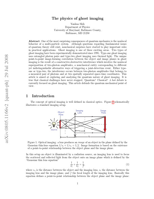
The Physics of Ghost Imaging

obj
dρo f (ρo ) δ (ρo +
ρi ) m
(2)
where I (ρi ) is the intensity in the image plane, ρo and ρi are 2-D vectors of the transverse coordinates in the object and image planes, respectively, and m = si /so is the magniﬁcation factor. In reality, limited by the ﬁnite size of the imaging system, we may never have a perfect pointto-point correspondence. The incomplete constructive-destructive interference turns the pointto-point correspondence into a point-to-“spot” relationship. The δ -function in the convolution of Eq. (2) will be replaced by a point-spread function: I (ρ i ) =
obj
dρo f (ρo ) somb
R ω ρi ρo + so c m
(3)
where the sombrero-like function, or the Airy disk, is deﬁned as somb(x) = 2J1 (x) , x
and J1 (x) is the ﬁrst-order Bessel function, and R the radius of the imaging lens, and R/so is known as the numerical aperture of an imaging system. The ﬁnite size of the spot, which is deﬁned by the point-spread function or the Airy disk, determines the spatial resolution of the imaging setup. It is clear from Eq. (3) that a larger imaging lens and shorter wavelength will result in a narrower point-spread function, and thus a higher spatial resolution of the image. Ghost imaging, in certain aspects, has the same basic feature of classical imaging, such as the unique point-to-point image-forming relationship between the object plane and the image plane. Diﬀerent from classical imaging, the radiation stopped on the imaging plane does not “come” from the object plane, instead it comes directly from the light source. More importantly, the image is observed in the joint detection between two independent photodetectors, one measures the scattered or transmitted light from the object, another measures light directly coming from the source at each point in the image plane. The point-to-point correlation is determined by the nonlocal behavior of a pair of photons: neither photon-one nor photon-two “knows” where to arrive. However, if one of them is observed at a point on the object plane, its twin must arrive at a unique corresponding point on the image plane. The ﬁrst ghost imaging experiment was demonstrated by Pittman et al. in 1995 [1] [2]. The schematic setup of the experiment is shown in Fig. 2. A continuous wave (CW) laser is used to pump a nonlinear crystal to produce an entangled pair of orthogonally polarized signal (e-ray of the crystal) and idler (o-ray of the crystal) photons in the nonlinear optical process of spontaneous parametric down-conversion (SPDC). The pair emerges from the crystal collinearly with ωs ∼ = ωi ∼ = ωp /2 (degenerate SPDC). The pump is then separated from the signal-idler pair by a dispersion prism, and the signal and idler are sent in diﬀerent directions by a polarization beam splitting Thompson prism. The signal photon passes through a convex lens of 400mm focal 2

pxe是什么呢（WhatisPXE）

pxe是什么呢（What is PXE）PXE是什么呢？PXE（预启动执行环境）是由英特尔公司开发的最新技术，工作于客户端/服务器的网络模式，支持工作站通过网络从远端服务器下载映像，并由此支持来自网络的操作系统的启动过程，其启动过程中，终端要求服务器分配IP地址，再用TFTP（Trivial File Transfer Protocol）或mtftp（组播文件传输协议）协议下载一个启动软件包到本机内存中并执行，由这个启动软件包完成终端基本软件设置，从而引导预先安装在服务器中的终端操作系统。

PXE可以引导多种操作系统，如：Windows 95 / 98 / 2000，Linux等。

PXE最直接的表现是，在网络环境下工作站可以省去硬盘，但又不是通常所说的无盘站的概念，因为使用该技术的PC在网络方式下的运行速度要比有盘PC快3倍以上。

当然使用PXE的PC也不是传统意义上的终端终端，因为使用了PXE的PC并不消耗服务器的CPU、RAM等资源，故服务器的硬件要求极低。

PXE工作原理：PXE（Preboot Execution Environment，远程引导技术）是RPL（远程初始程序加载，远程启动服务）的升级产品。

它们的不同之处为：RPL是静态路由，PXE是动态路由。

不难理解：RPL是根据网卡上的ID号加上其它的记录组成的一个帧向服务器发出请求，而服务器那里早已经有了这个ID数据，匹配成功则进行远程启动；PXE则是根据服务器端收到的工作站MAC地址（就是网卡号），使用DHCP服务给这个MAC地址指定一个IP地址，每次重启动可能同一台工作站有与上次启动有不同的IP，即动态分配地址下面以工作站引导过程说明PXE。

的原理：1、工作站开机后，PXE BootROM（自启动芯片）获得控制权之前先做自我测试，然后以广播形式发出一个请求找到帧。

2、如果服务器收到工作站所送出的要求，就会送回DHCP回应，内容包括用户端的IP地址，预设通讯通道，及开机映像文件否则，服务器会忽略这个要求。

MATRICES WITH MAXIMUM UPPER MULTIEXPONENTS IN THE CLASS OF PRIMITIVE, NEARLY REDUCIBLE MATR

TAIWANESE JOURNAL OF MATHEMATICSVol.2,No.2,pp.181-190,June1998MATRICES WITH MAXIMUM UPPER MULTIEXPONENTSIN THE CLASS OF PRIMITIVE,NEARLY REDUCIBLE MATRICESZhou BoAbstract.B.Liu has recently obtained the maximum value for the k thupper multiexponents of primitive,nearly reducible matrices of ordern with1≤k≤n.In this paper primitive,nearly reducible matriceswhose k th upper multiexponents attain the maximum value are com-pletely characterized.1.IntroductionA square Boolean matrix A is primitive if one of its powers,A k,is the matrix J of all1’s for some integer k≥1.The smallest such k is called the primitive exponent of A.The matrix A is reducible if there is a permutation matrix P such thatP t AP= A10X A2 ,where A1and A2are square and nonvacuous;otherwise A is irreducible.The matrix A is nearly reducible if A is irreducible but each matrix obtained from A by replacing any nonzero entry by zero is reducible.It is well known that there is an obvious one-to-one correspondence between the set B n of n by n Boolean matrices and the set of digraphs on n vertices. Given A=(a ij)∈B n,the associated digraph D(A)has vertex set V(D(A))= {1,2,...,n},and arc set E(D(A))={(i,j):a ij=1}.A is primitive if and only if D(A)is strongly connected and the greatest common divisor(gcd for short)of all the distinct cycle lengths of D(A)is1,and A is nearly reducible if and only if D(A)is a minimally strongly connected digraph.We say a digraph 0Received May9,1996;revised September10,1997.Communicated by G.J.Chang.1991Mathematics Subject Classiﬁcation:05C50,15A33.Key words and phrases:Primitive matrix,nearly reducible matrix,upper multiexponent.181182Zhou Bois primitive with primitive exponentγif it is the associated digraph of some primitive matrix with primitive exponentγ.Now we give the deﬁnition of the upper multiexponent for a primitive digraph,which was introduced by R.A.Brualdi and B.Liu[1].Let D be a primitive digraph on n vertices.The exponent of a subset X⊆V(D)is the smallest integer p such that for each vertex i of D there exists a walk from at least one vertex in X to i of length p(and of course every length greater than p,since D is strongly connected).We denote it by exp D(X).The numberF(D,k)=max{exp D(X):X⊆V(D),|X|=k}is called the kth upper multiexponent of D.Clearly F(D,1)is the primitive exponent of D.Hence the k th upper mul-tiexponent of a primitive digraph is a generalization of its primitive exponent.Let A be an n×n primitive matrix,and let k be an integer with1≤k≤n. The k th upper multiexponent of A is the k th upper multiexponent of D(A), denoted by F(A,k).Thus F(A,k)=F(D(A),k).Clearly F(A,k)is the smallest power of A for which no set of k rows has a column consisting of all zeros.In[2]B.Liu obtained the maximum value for the k th upper multiexpo-nents of primitive,nearly reducible matrices of order n with1≤k≤n.In this paper,we provide a complete characterization of matrices in the class of n×n primitive,nearly reducible matrices whose k th upper multiexponents for 1≤k≤n attain the maximum value.Using the correspondence between matrices and digraphs,we express the results in the digraph version.2.Main ResultsWeﬁrst give several lemmas that will be used.Lemma1.[3].Let D be a primitive digraph on n vertices,1≤k≤n−1, and let h be the length of the shortest cycle of D.ThenF(D,k)≤n+h(n−k−1).LetF(n,k)= n2−4n+6,k=1;(n−1)2−k(n−2),2≤k≤n.The following lemma has been proved in[2]for n≥5.For n=4it can be checked readily.Matrices with Maximum Upper Multiexponents183 Lemma2.[2].F(D n−2,k)=F(n,k),n≥4,where D n−2is the digraph given by Fig.1.Lemma3.[1].Let D be a primitive digraph with n vertices and let h and t be respectively the smallest and the largest cycle lengths of D.ThenF(D,n−1)≤max{n−h,t}.Let P MD n be the set of all primitive,minimally strongly connected di-graphs with n vertices.The following theorem has recently been proved by B. Liu.Theorem1.[2].Max{F(D,k):D∈P MD n}=F(n,k),1≤k≤n.A problem that deserves investigation is to characterize the extreme di-graphs,or the digraphs in P MD n whose k th upper multiexponents assume the maximum value F(n,k).Obviously,for any D∈P MD n,F(D,n)=F(n,n)=1.We are going to consider the case1≤k≤n−1.Theorem2.Let D∈P MD n,1≤k≤n−1,n≥4.Then for1≤k≤n−2,F(D,k)=F(n,k)if and only if D∼=D n−2,where D n−2is the digraph given by Fig.1;F(D,n−1)=F(n,n−1)=n−1if and only if D∼=D n,s with1≤s≤n−3and gcd(n−1,s+1)=1,where D n,s is the digraph given by Fig.2.FIG.1.183184Zhou BoFIG.2.Remark.When s=n−3,D n,s is the digraph D n−2for n≥4.Proof.We begin the proof with the case k=n−1ﬁrst. Suppose D∼=D n,s.For i=2,3,...,s(s>1),any walk from the vertex i to the vertex n−1has a length of the form n−1−i+a(n−1)+b(s+1),where a and b are non-negative integers.Consider the equation n−1−i+a(n−1)+b(s+1)= n−2,i.e.,a(n−1)+b(s+1)=i−1.Since i≤s≤−3,we have a=0,b=0, which is imposssible.Hence there is no walk of length n−2from the vertex i to the vertex n−1for i=2,3,...,s.For i=s+1,...,n−1(s≥1),we have the same conclusion as above.Also it is easy to see that there is no walk of length n−2from the vertex n to the vertex n−1.Now take X0=V(D)\{1}. There does not exist any walk from a vertex in X0to the vertex n−1of lengthn−2.Hence exp Dn,s (X0)≥n−1.By the deﬁnition of the(n−1)th uppermultiexponent and Theorem1it follows thatF(D,n−1)=F(D n,s,n−1)=n−1.Conversely,suppose F(D,n−1)=n−1.Let h and t be respectively the smallest and the largest cycle lengths of D.D cannot have a cycle of length n,because,if so,the digraph is still strongly connected after the removal of any arc lying outside such cycle,contradicting the fact that D is minimally strongly connected.Similarly,we can show that D has no loops.So we have 2≤h≤n−2,t≤n−1.By Lemma3we obtainn−1=F(D,n−1)≤max{n−h,t},which implies t=n−1.Suppose D contains a cycle of length n−1whose arcs are(i,i+1)for i=1,2,...,n−2,and(n−1,1).By the strong connectedness of D there exist u and v(u and v may be equal)in{1,2,...,n−1}such thatMatrices with Maximum Upper Multiexponents185 (u,n)and(n,v)are arcs in D.Without loss of generality we assume that v=1.Thus D contains a subdigraph D n,u with1≤u≤n−3.Since D is minimally strong,it is easy to see that D has no arcs other than those in D n,u.It follows from the primitivity of D that gcd(n−1,u+1)=1.Now we turn to the case1≤k≤n−2.The case k=1is proved in[4]. Suppose2≤k≤n−2.If D∼=D n−2,by Lemma2we have F(D,k)=F(n,k). Conversely,suppose F(D,k)=F(n,k)and let h be the length of the shortest cycle in D.Since D is primitive,it has at least two diﬀerent cycle lengths. In addition,D has no cycles of length n,being a minimally strong connected digraph of order n.It follows that h≤n−2.If h=n−2,then the set of all distinct cycle lengths of D is{n−2,n−1}. By the minimally strong connectedness of D,it follows that D∼=D n−2.We are going to show that it is impossible to have h≤n−3.We divide our argument into two cases.Case1:2≤k<n−2.If h≤n−3,applying Lemma1we haveF(D,k)≤n+h(n−k−1)≤n+(n−3)(n−k−1)=(n−1)2−k(n−2)−(n−k−2)<(n−1)2−k(n−2)=F(n,k),a contradiction.Case2:k=n−2.If h≤n−4,by Lemma1,F(D,k)≤n+h(n−k−1)≤n+(n−4)(n−k−1)=2n−4<2n−3=F(n,k),a contradiction.If h=n−3,observing that D cannot have loops,we have h≥2and n≥5.If n=5,then h=2.Since D cannot have a cycle of length5and D is primitive,D must have a cycle of length3.It follows from the fact that D is minimally strongly connected that D is isomorphic with D1or D2or D3as displayed in Fig.3.In all such cases,it is easy to verify that we have F(D,1)≤6.Hence F(D,n−2)=F(D,3)≤F(D,1)≤6<7=F(5,3), which is a contradiction.Now suppose h=n−3and n>5.Since D cannot have a cycle of length n,by the primitivity of D,D must contain a cycle of length of n−2or n−1.185186Zhou BoFIG.3.If there is a walk of length t from vertex j to vertex i,we say that j is a t-in vertex of i.And the set of all t-in vertices of i in D is denoted by R D(t,i).Case2.1:D has no cycles of length n−1.Then D must have a cycle of length n−2.Take a cycle C of D of length n−2.Then D has precisely two vertices,say,x,y,lying outside C.We divide this situation into the following two subcases.(1)D contains one of the arcs(x,y)or(y,x).Say,D contains the arc (x,y).Then(y,x)cannot be an arc of D;otherwise,n−3=h=2and so n=5,which is a contradiction.By the strong connectedness of D,there must exist vertices u,v of C(the cycle of length n−2)such that(u,x)and(y,v) are both arcs of D.If u=v,then n−3=h=3,so we have n=6and D is the digraph D16−3.If u=v,then since D has precisely two cycles,of lengths n−2and n−3respectively,it will follow that D is isomorphic with D1n−3(n≥7).D1n−3(n≥6)is given by Fig.4.Suppose D=D1n−3.For n≥6,we describe R D(2n−5,i)explicitly:R D(2n−5,1)={n,1,2},R D(2n−5,i)={i−1,i,i+1},i=2,3,...,n−4,R D(2n−5,n−3)={n−4,n−3,n−2,n−1},R D(2n−5,n−2)={n−2,n−1,n,1},R D(2n−5,n−1)={n−4,n−3,n−2,n−1},R D(2n−5,n)={n−2,n−1,n,1}.Matrices with Maximum Upper Multiexponents187FIG.4.It is clear that each vertex has at least three(2n−5)-in vertices in D,and so exp D(X)≤2n−5for any set of n−2vertices.It follows from the deﬁnition of the(n−2)th upper multiexponent that F(D,n−2)≤2n−5<2n−3= F(D,n−2),which is a contradiction.(2)Neither(x,y)nor(y,x)is an arc of D.By the strong connectedness of D,there must exist vertices u,v,u and v of C such that(u,x),(x,v),(u ,y) and(y,v )are arcs of D.We have u=v and u =v ;otherwise,n−3=h=2 and so n=5,which is a contradiction.Also neither(u,v)nor(u ,v )is an arc of C;otherwise D has a cycle of length n−1,which is a contradiction. Suppose that uu1u2···u r v and u v1v2···v t v are two paths of C,of lengths r+1and t+1respectively,where r≥1and t≥1.If r=t=1,then by the minimally strong connectedness of D,D has no cycles of length h=n−3, which is a contradiction.If r≥3or t≥3,then there is a cycle with length less than h=n−3,which is also a contradiction.Hence we have r=2 or t=2.So D contains a subdigraph which is isomorphic with D(n−1)−2 (see Fig.1for D n−2).Assume D(n−1)−2is a subdigraph of D.Note that V(D(n−1)−2)={1,2,...,n−1}.By the strong connectedness of D,there exists a vertex j∈{1,2,...,n−1}such that(j,n)is an arc of D.Let X⊆V(D)with|X|=n−2.For each vertex1,2,...,n−1,there is a walk to the vertex from a vertex in X\{n}of length exp D(n−1)−2(X\{n})(and hence also every length greater).This is because,each such vertex belongs to the subgraph D(n−1)−2.Note thatexp D(n−1)−2(X\{n})≤ F(D(n−1)−2,n−2)=n−2,n∈X;F(D(n−1)−2,n−3)=2n−5,n∈X.187188Zhou BoSo exp D(n−1)−2(X\{n})≤2n−5whether n∈X or n∈X.Thus for everyinteger t≥2n−5,and for each vertex1,2,...,n−1,there is a walk to the vertex from a vertex in X\{n}of length t.Since j∈{1,2,...,n−1}and (j,n)is an arc of D,it follows that there is a walk to the vertex n from a vertex in X\{n}of length t+1for every integer t≥2n−5.So we have proved that there is a walk to each vertex of D from a vertex in X\{n}of length t+1for every integer t≥2n−5.This implies thatexp D(X)≤exp D(X\{n})≤2n−4<2n−3.By the deﬁnition of the(n−2)th upper multiexponent,we have F(D,n−2)< 2n−3=F(n,n−2),which is a contradiction.Case2.2:D has a cycle of length of n−1.Since h=n−3,D also has a cycle of length n−3.By the minimally strong connectedness of D,one can readily show that in this case D is composed of precisely two cycles,of lengths n−1and n−3respectively.But gcd{n−1,n−3}=1,so n is even,and D must be isomorphic with D2n−3(n≥6),where D2n−3is given by Fig.5.Suppose D=D2n−3.We haveR D(2n−4,1)={n,1,3},R D(2n−4,2)={2,4,n−3,n−1},R D(2n−4,3)={n,1,3,5},R D(2n−4,i)={i−2,i,i+2},i=4,...,n−3,R D(2n−4,n−2)={n−4,n−3,n−2,1},R D(2n−4,n−1)={n−3,n−1,2},R D(2n−4,n)={n−4,n,1}.By similar arguments as for the case D∼=D1n−3,we get F(D,n−2)≤2n−4<2n−3=F(n,n−2),which is also a contradiction.Now we have proved that it is impossible to have h≤n−3.Thus the proof of the theorem is completed.Theorem2gives complete characterizations of the extreme digraphs in the class of primitive,minimally strong digraphs of order n whose k th(1≤k≤n−1)upper multiexponents assume the maximum value.Note that there is not any digraph D in P MD n with F(D,1)=m if n2−5n+9<m<F(n,1),or n2−6n+12<m<n2−5n+9for n≥4(see [4]).As a by-product of the proof of Theorem2we have a similar result.Corollary1.Let k and n be integers.If2≤k≤n−3,then for any integer m satisfying n+(n−3)(n−k−1)<m<F(n,k),there is no digraph D∈P MD n such that F(D,k)=m.Matrices with Maximum Upper Multiexponents189FIG.5.D2(n is even,n≥6).n−3This corollary tells us that there are gaps in the set of k th upper multiex-ponents of digraphs in P MD n(1≤k≤n−3).Corollary2.The number of non-isomorphic extreme digraphs in P MD n with the(n−1)th upper multiexponent equal to n−1(n≥4)isφ(n−1)−1, whereφis Euler’s totient function.Finally,we point out that the maximum value for the k-exponents of primi-tive,nearly reducible matrices is also obtained in[2],and we have characterized the corresponding extreme matrices in another paper.AcknowledgementThe author would like to thank Professor B.Liu and Professor Gerard J.Chang for help and encouragement,and the referees for their numerous suggestions,which have resulted in a great improvement in the paper.References1.R.A.Brualdi and B.Liu,Generalized exponents of primitive directed graphs,J.Graph Theory14(1990),483-499.2. B.Liu,Generalized exponents of primitive,nearly reducible matrices,Ars Com-bin.to appear.3. B.Liu and Q.Li,On a conjecture about the generalized exponent of primitivematrices,J.Graph Theory18(1994),177-179.4.J.A.Ross,On the exponent of a primitive,nearly reducible matrix II,SIAMJ.Discrete Math.3(1982),395-410.189190Zhou Bo5. A.L.Dulmage and N.S.Mendelsohn,Gaps in the exponent set of primitivematrices,Illinois J.Math.8(1964),642-656.Department of Mathematics,South China Normal UniversityGuangzhou510631,China。

Magnetic ordering in Gd2Sn2O7 the archetypal Heisenberg pyrochlore antiferromagnet

a r X i v :c o n d -m a t /0602138v 1 [c o n d -m a t .m t r l -s c i ] 6 F eb 2006LETTER TO THE EDITORMagnetic ordering in Gd 2Sn 2O 7:the archetypal Heisenberg pyrochlore antiferromagnet A S Wills,1,2M E Zhitomirsky,3B Canals,4J P Sanchez,3P Bonville,5P Dalmas de R´e otier 3and A Yaouanc 31Department of Chemistry,University College London,20Gordon Street,London,WC1H 0AJ,UK 2Davy-Faraday Research Laboratory,The Royal Institution of Great Britain,London W1S 4BS,UK 3Commissariat `a l’Energie Atomique,DSM/DRFMC/SPSMS,38054Grenoble,France 4Laboratoire Louis N´e el,CNRS,BP-166,38042Grenoble,France 5Commissariat `a l’Energie Atomique,DSM/SPEC,91191Gif-sur-Yvette,France Abstract.Low-temperature powder neutron diﬀraction measurements are performed in the ordered magnetic state of the pyrochlore antiferromagnet Gd 2Sn 2O 7.Symmetry analysis of the diﬀraction data indicates that this compound has the ground state predicted theoretically for a Heisenberg pyrochlore antiferromagnet with dipolar interactions.The diﬀerence in magnetic structures of Gd 2Sn 2O 7and of nominally analogous Gd 2Ti 2O 7is found to be determined by a speciﬁc type of third-neighbor superexchange interaction on the pyrochlore lattice between spins across empty hexagons.Frustration or inability to simultaneously satisfy all independent interactions [1]has become an important theme in condensed matter research,coupling at the fundamental level a wide range of phenomena,such as high-T c superconductivity,the folding of proteins and neural networks.Magnetic crystals provide one of the simplest stages within which to explore the inﬂuence of frustration,particularly when it arises as a consequence of lattice geometry,rather than due to disorder.For this reason,geometrically frustrated magnetic materials have been the objects of intense scrutiny for over 20years [2].Particular interest has been focussed on kagom´e and pyrochlore (see Fig.1)geometries of vertex-sharing triangles and tetrahedra respectively.Model materials with their structures display a wide range of exotic low-temperature physics,such as spin ice [3],spin liquids [4],topological spin glasses [5],heavy fermion [6],and co-operative paramagnetic ground states [7].Research into these systems was spawned from studies of the archetypal geometrically frustrated system—the Heisenberg pyrochlore antiferromagnet,which in the classical limit was shown theoretically to possess a disordered ground state.Raju and co-workers found that the Heisenberg pyrochlore antiferromagnet with dipolar interactions has an inﬁnite number of degenerate spin conﬁgurations near the mean-ﬁeld transitiontemperature,which are described by propagation vectors [hhh ][8].Later,Palmer and Chalker showed that quartic terms in the free energy lift this degeneracy and stabilize a four-sublattice state with the ordering vector k =(000)(the PC state)[9].Among various pyrochlore materials Gd 2Ti 2O 7and Gd 2Sn 2O 7are believed to be good realizations of Heisenberg antiferromagnets.Indeed,the Gd 3+ion has a half-ﬁlled 4f -shell with nominally no orbital moment.A strong intrashell spin-orbitFigure 1.Pyrochlore lattice of vertex sharing tetrahedra.Next-neighborexchanges are shown by long-dashed line.coupling mixes,however,8S7/2and6P7/2states leading to a sizable crystal-ﬁeld splitting.Recent ESR measurements on dilute systems gave comparable ratios of the single-ion anisotropy constant D>0to the nearest-neighbor exchange J for the two compounds:D/J∼0.7[10].This corresponds to a planar anisotropy for the ground state.Magnetic properties of the stannate and the titanate would be expected, therefore,to be very similar.In this light,the contrasts between the low-temperature behavior of Gd2Sn2O7and that of the analogous titanate are remarkable.While the titanate displays two magnetic transitions,at∼0.7and1K,to structures with the ordering vector k= 121-20000-12000-400040001200020000 28000 36000 4400052000600002 θ (°)I n t e n s i t y (a .u .)Figure 2.Fit to the magnetic diﬀraction pattern of Gd 2Sn 2O 7obtained fromthe ψ6basis state by Rietveld reﬁnement.The dots correspond to experimentaldata obtained by subtraction of that measured in the paramagnetic phase (1.4K)from that in the magnetically ordered phase (0.1K).The solid line correspondsto the theoretical prediction and the line below to the diﬀerence.Positions forthe magnetic reﬂections are indicated by vertical markers.to the linear combination observed in the model XY pyrochlore antiferromagnet Er 2Ti 2O 7[11],c Γ7+to the manifold of states proposed as the ground states for the Heisenberg pyrochlore antiferromagnet with dipolar terms (the PC ground state),and c Γ9+to a spin-ice like manifold observed in the non-collinear ferromagnetic pyrochlores such as Dy 2Ti 2O 7[3].While the phase transition in Gd 2Sn 2O 7has been shown to be ﬁrst order which allows ordering according to several irreducible corepresentations,it is commonly found that the terms which drive the transition to being ﬁrst order are relatively weak and cause only minor perturbation to the resultant magnetic structure.Following this,we examined whether the models detailed above could ﬁt the observed magnetic neutron diﬀraction spectrum.The goodness of ﬁt parameter,χ2,for the ﬁt to models characterised by each irreducible corepresentation are:c Γ3+(69.0),c Γ5+(35.6),c Γ7+(5.18),c Γ9+(13.6).We ﬁnd that the magnetic scattering can only be well modeled by c Γ7+,the PC state in which the moments of a given Gd tetrahedron are parallel to the tetrahedron’s edges.In this state each moment is ﬁxed to be perpendicular to the local 3-fold axis of each tetrahedron,consistent with M¨o ssbauer data [13,14].Powder averaging leads to the structures ascribed to ψ4,ψ5and ψ6being indistinguishable by neutron diﬀraction and prevents contributions of the individual basis vectors from being reﬁned.For this reason only ψ6was used in the reﬁnement and the ﬁnal ﬁt is presented in Figure 2.While the value of the ordered moment,6(1)µB /Gd 3+,obtained by scaling the magnetic and nuclear peaks is imprecise due to the uncertainty over the isotopic composition of the Gd and the concomitant neutron absorption,it is consistent with the free-ion value (7µB )and that measured by M¨o ssbauer spectroscopy [13].Realization of the PC state in Gd 2Sn 2O 7,but not in Gd 2Ti 2O 7,indicates that the magnetic Hamiltonian of the titanate contains additional terms.C´e pas and Shastry[20]have suggested that next-neighbor exchange may stabilize magnetic ordering at k =(121Figure3.The magnetic structure basis vectors labelled according to the diﬀerentirreducible corepresentations for Gd2Sn2O7.tiny.Also,possible exchange paths were not investigated in their work as both types of third-neighbor exchange(Fig.1)were assumed to be equal.The pyrochlore A2B2O7structure has two inequivalent oxygen sites:O1at(x,18)and O2at(38,3J 31J 2(q 0 0)Figure 4.Instability wave-vectors for diﬀerent values of second-and third-neighbor exchange constants for a Heisenberg pyrochlore antiferromagnet withdipolar interactions.Incommensurate states are indicated by nonzero componentsof the wave-vectors.All transition lines are of the ﬁrst-order.ˆH = i,j J ij S i ·S j +D i (n i ·S i )2+(gµB )2 i,j S i ·S j r 5ij ,where the superexchange J ij extends up to the third-neighbor pairs of spins and D >0is a single-ion anisotropy.The strength of the dipolar interaction between nearest-neighborspinsEdd =(gµB )2/(a√212).In such a case,a ﬂuctuationdriven ﬁrst-order transition is expected to the PC state [9,22].The diagram of possible ordering wave-vectors for a restricted range of J 31and J 2are presented in Fig.4.It contains two commensurate states with k =(000)and k =(121212)magnetic structure,which exists in a wide range0<J 31<0.335J .In contrast,a small ferromagnetic J 2within a narrow window −0.04J <J 2<0is needed to obtain the same ordering without J 31.In the whole range of parameters,the eigenstate with k =(121212)vector.We have also veriﬁed that the second type of third-neighbor exchange J32does not lead to further stabilization of the(121212)states.In conclusion,the occurrence of the PC state in Gd2Sn2O7but not in Gd2Ti2O7 indicates that the latter possesses additional contributions,which we identify as a type of third–neighbor exchange.Gd2Sn2O7presents,therefore,the only accurate realization of the Heisenberg pyrochlore antiferromagnet with dipolar interactions.We are grateful to A.Forget for preparing the160Gd enriched sample and to the ILL for provision of neutron time.ASW would like to thank the Royal Society and EPSRC(grant number EP/C534654)forﬁnancial support.References[1]Anderson P W1973Mat.Res.Bull.8153[2]Villain J1979Z.Phys.B3331[3]Harris M J,Bramwell S T,McMorrow D F,Zeiske T and Godfrey K W1997Phys.Rev.Lett.792554[4]Ballou R,Leli`e vre-Berna E and F˚ak B1996Phys.Rev.Lett.77790[5]Wills A S,Depuis V,Vincent E and Calemczuk R2000Phys.Rev.B629264(R)[6]Urano C,Nohara M,Kondo S,Sakai F,Takagi H,Shiraki T and Okubo T2000Phys.Rev.Lett.851052[7]Gingras M J P,den Hertog B C,Faucher M,Gardner J S,Dunsiger S R,Chang L J,GaulinB D,Raju N P and Greedan J E2000Phys.Rev.B626496[8]Raju N P,Dion M,Gingras M J P,Mason T E and Greedan J E1999Phys.Rev.B5914489[9]Palmer S E and Chalker J T2000Phys.Rev.B62488[10]Glazkov V N,Zhitomirsky M E,Smirnov A I,Krug von Nidda H-A,Loidl A,Marin C andSanchez J P2005Phys.Rev.B72020409(R);Glazkov V N,Smirnov A I,Sanchez J P, Forget A,Colson D and Bonville P2005Preprint cond-mat/0510575[11]Champion J D M,Wills A S,Fennell T,Bramwell S T,Gardner J S and Green M A2001Phys.Rev.B64140407[12]Stewart J R,Ehlers G,Wills A S,Bramwell S T and Gardner J S2004J.Phys.:Condens.Matter16L321[13]Bonville P,Hodges J A,Ocio M,Sanchez J P,Vulliet P.,Sosin S and Braithwaite D2003J.Phys.Condens.Matter.157777[14]Bertin E,Bonville P,Bouchaud J-P,Hodges J A,Sanchez J P and Vulliet P2002Eur.Phys.J.B27347[15]Wills A S2000Physica B276680;progam available from ftp.ill.fr/pub/dif/sarah/[16]Rodriguez-Carvajal J1993Physica B19255[17]Kovalev O V1993Representations of the Crystallographic Space Groups Edition2(Gordon andBreach Science Publishers,Switzerland)[18]The corepresentations are real and are labelled according to the notation of Kovalev[17]forthe parent representation and whether the antiunitary halﬁng group was created according to the d(a)=±δ(aa−1)β,where d(a)is the matrix representitive of antiunitary symmetryelement a,δ(aa−10)is the matrix representitive of unitary symmetry element aa−1,a0is anantiunitatry generating element andβis an unitary matrix.[19]Greedan J E,O’Reilly A H and Stager C V1987Phys.Rev.B358770[20]C´e pas O.and Shastry B.M.2004Phys.Rev.B69184402[21]Kennedy B J,Hunter B A and Howard C J1997J.Solid State Chem.13058;Helean K B,Ushakov S V,Brown C E,Navrotsky A,Lian J,Ewing R C,Farmer J M and Boatner L A 2004ibid.1771858[22]Brazovskii S A1975Zh.´Eksp.Teor.Fiz.68,175[Sov.Phys.JETP4185];Cepas O,Young AP and Shastry B S2005Phys.Rev.B72184408。

1、下载文档前请自行甄别文档内容的完整性，平台不提供额外的编辑、内容补充、找答案等附加服务。
2、"仅部分预览"的文档,不可在线预览部分如存在完整性等问题,可反馈申请退款(可完整预览的文档不适用该条件!)。
3、如文档侵犯您的权益，请联系客服反馈,我们会尽快为您处理(人工客服工作时间：9:00-18:30)。

Fig. 1. A purine–pyrimidine graph.
Байду номын сангаас
ð2:1:6Þ
ðb þ diÞ ! A; ðd þ biÞ ! G; ðb À diÞ ! T; ðd À biÞ ! C
or
reih1 ! A; reih2 ! G; reih3 ! T; reih4 ! C;
pﬃﬃﬃﬃﬃﬃﬃﬃﬃﬃﬃﬃﬃﬃﬃ
1. Introduction
Mathematical analysis of the large volume genomic DNA sequence data is one of the challenges for bioscientists. In recent years several novel graphical representations of DNA sequences have outlined in the literature [1–10,14–16]. Nandy [1] presented a graphical representation by assigning A (adenine), G (guanine), T (thymine), and C (cytosine) to the four direction, (Àx), (+x), (Ày), (+y), respectively. Such a representation of DNA is accompanied by some loss of information associated with crossing and overlapping of the resulting curve by itself, other ones allow full reconstruction of the primary sequence from the given graphical representation, but both serve equally to facilitate construction of DNA sequence invariants to be used as a tool in comparative studies of DNA. In contrast to DNA, there are no similar approaches addressing graphical representation of protein sequences, except
Received 19 June 2005; in ﬁnal form 19 July 2005 Available online 30 August 2005
Abstract
Graphical representation of DNA provides a simple way of viewing, sorting and comparing various gene structures. A 2-D graphical representation of protein sequences based on nucleotide triplet codons has been derived for similarity analysis of protein sequences. This approach is based on a graphical representation of triplets of DNA in which the interior of the left half plane of the complex plane is used to accommodate 64 sites for the 64 codons. We associate a directed curve, numerical value, or matrix with a protein as a descriptor. The approach is illustrated on the Homo sapiens X-linked nuclear protein (ATRX) gene. Ó 2005 Elsevier B.V. All rights reserved.
* Corresponding author. Fax: +86 411 84706100. E-mail addresses: bﬂ0219@, bf18611@ (F. Bai),
wangtm@ (T. Wang).
for very recent outline of highly condensed graphical representation of proteins [11,12]. Randic et al. [13] present a novel graphical representation of proteins that produces an 8 · 8 tabular representation of 64 codons, and the corresponding table of amino acids, both of which allow the construction of associated zigzag curves that lead to a numerical characterization of proteins.
where
r¼
b2 þ d2;
hk
¼
arg
tan
d b
;
k ¼ 1; 2; 3; 4,
b and d is non-zero positive real number, A and T are
conjugate, G and C are conjugate too, namely, A ¼ T; G ¼ C, so A + T + C + G = 2(b + d). In this
the following conditions:
8 >>><
ðb ðd
þ þ
d iÞ biÞ
yðjÞ ¼ >>>: ðb À diÞ
ðd À biÞ
if j ¼ A; if j ¼ G; if j ¼ T; if j ¼ C;
ð2:1:1Þ
(j = 0,1,2, Á Á Á ,n, where n is the length of the DNA sequence being studied)
0009-2614/$ - see front matter Ó 2005 Elsevier B.V. All rights reserved. doi:10.1016/j.cplett.2005.08.011
F. Bai, T. Wang / Chemical Physics Letters 413 (2005) 458–462
P~j ! ðbaj þ dgj þ btj þ dcjÞ þ ðdaj þ bgj À dtj À bcjÞi; ð2:1:2Þ
where aj, gj, tj and cj are the cumulative occurrence numbers of A, G, T and T, in the subsequence from the lst base to the jth base, respectively, We deﬁne a0 = g0 = t0 = c0 = 0, then we have properties as follows:
Property 1. For a given DNA sequence there is a unique x(n) corresponding to it.
Proof. Let bj + dji be the vector of the curve x(n) in the complex plane corresponding to the jth base of DNA sequence, then we have
2. 2-D representation of DNA triples
2.1. 2-D representation of DNA sequences
As shown in Fig. 1, we construct a purine–pyrimidine graph on the left half of the complex plane, with purines (A and G) in the ﬁrst quadrant and pyrimidines (T and C) in the fourth quadrant. The unit vectors representing four nucleotides A, G, C, and T are as follows:
ðbj þ djiÞ ¼ ðbaj þ dgj þ btj þ dcjÞ þ ðdaj þ bgj À dtj À bcjÞi
or
ð2:1:3Þ
Because b and d is non-zero positive real number and
Fenglan Bai a,*, Tianming Wang a,b
a Department of Applied Mathematics, Dalian University of Technology, LiaoNing, Dalian 116024, China b Department of Mathematics, Hainan Normal University, Haikou 571158, China
way, we can reduce a DNA sequence into a series of vec-