getting started with stata for windows
Stata软件的参考手册列表说明书
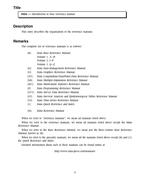
TitleDescriptionThis entry describes the organization of the reference manuals.RemarksThe complete list of reference manuals is as follows:[R]Stata Base Reference ManualVolume1,A–HVolume2,I–PVolume3,Q–Z[D]Stata Data-Management Reference Manual[G]Stata Graphics Reference Manual[XT]Stata Longitudinal-Data/Panel-Data Reference Manual[MI]Stata Multiple-Imputation Reference Manual[MV]Stata Multivariate Statistics Reference Manual[P]Stata Programming Reference Manual[SVY]Stata Survey Data Reference Manual[ST]Stata Survival Analysis and Epidemiological Tables Reference Manual[TS]Stata Time-Series Reference Manual[I]Stata Quick Reference and Index[M]Mata Reference ManualWhen we refer to“reference manuals”,we mean all manuals listed above.When we refer to the reference manuals,we mean all manuals listed above except the Mata Reference Manual.When we refer to the Base Reference Manual,we mean just the three-volume Base Reference Manual,known as[R].When we refer to the specialty manuals,we mean all the manuals listed above except[R]and[I], the Quick Reference and Index.Detailed information about each of these manuals can be found online at/manuals/12intro—Introduction to base reference manualintro—Introduction to base reference manual3mmarize varlist if in weight ,optionsoptions descriptionetail display additional statisticsmeanormat use variable’s display formatsepvarlist may contain factor variables;see[U]11.4.3Factor variables.varlist may contain time-series operators;see[U]11.4.4Time-series varlists.by is allowed;see[D]by.aweight s,fweight s,and iweight s are allowed.However,iweight s may not be used with the detailoption;see[U]11.1.6weight.Items in the typewriter-style font should be typed exactly as they appear in the diagram, although they may be abbreviated.Underliningmmarize may be abbreviated su,sum,summ,etc.,or it may be spelled out completely.Items in the typewriter font that are not underlined may not be abbreviated.Square brackets denote optional items.In the syntax diagram above,varlist,if,in,weight,and the options are optional.The options are listed in a table immediately following the diagram,along with a brief description of each.Items typed in italics represent arguments for which you are to substitute variable names,observation numbers,and the like.The diagrams use the following symbols:#Indicates a literal number,e.g.,5;see[U]12.2Numbers.Anything enclosed in brackets is optional.At least one of the items enclosed in braces must appear.|The vertical bar separates alternatives.%fmt Any Stata format,e.g.,%8.2f;see[U]12.5Formats:Controlling how data are displayed. depvar The dependent variable in an estimation command;see[U]20Estimation and postesti-mation commands.exp Any algebraic expression,e.g.,(5+myvar)/2;see[U]13Functions and expressions.filename Anyfilename;see[U]11.6File-naming conventions.indepvars The independent variables in an estimation command;see[U]20Estimation and postestimation commands.newvar A variable that will be created by the current command;see[U]11.4.2Lists of new variables.4intro—Introduction to base reference manual£...£SE/Robust£...£Maximizationintro—Introduction to base reference manual5。
使用Stata进行数据处理和分析
使用Stata进行数据处理和分析第一章:Stata的介绍和安装Stata是一款统计软件,广泛应用于数据处理和分析领域。
本章将介绍Stata的基本功能和特点,并介绍如何安装Stata软件。
1.1 Stata的基本功能Stata具有数据管理、统计分析、图形绘制和模型拟合等功能。
数据管理功能包括数据输入、清理、转换和合并等操作;统计分析功能包括描述性统计、假设检验、回归分析和生存分析等方法;图形绘制功能可以用于可视化数据;而模型拟合功能可以进行回归、时间序列和面板数据等模型拟合。
1.2 Stata的特点Stata具有高度的统一性和完整性,适合处理小样本和大样本数据。
它提供了丰富的内置统计命令和扩展命令,可满足各种数据处理和分析的需求。
此外,Stata还具备灵活的数据处理能力和简洁的语法结构,方便用户进行数据操作和分析。
1.3 Stata的安装Stata支持Windows、Mac和Linux操作系统。
用户可以从Stata 官方网站购买软件并进行在线安装,或者通过光盘进行离线安装。
安装过程简单,用户只需按照安装向导的指示进行操作即可。
第二章:数据的导入和清洗本章将介绍如何使用Stata导入外部数据集并进行数据清洗。
2.1 数据导入Stata支持导入多种数据格式,如CSV、Excel和SPSS等。
用户可以使用命令“import”或点击菜单栏中的“File”-“Import”进行数据导入。
导入后,可以使用“describe”命令查看数据的基本信息。
2.2 数据清洗数据清洗是数据处理的重要环节,目的是提高数据的质量和可用性。
Stata提供了一系列数据清洗命令,如数据排序、缺失值处理和异常值检测等。
用户可以利用这些命令进行数据清洗,确保数据的准确性和完整性。
第三章:数据的转换和合并本章将介绍Stata中数据的转换和合并操作。
3.1 数据转换数据转换是将数据从一种形式转换为另一种形式的过程。
Stata 提供了多种数据转换命令,如变量生成、变量重编码和重塑数据等。
Stata 使用手册说明书

1Read this—it will helpContents1.1Getting Started with Stata1.2The User’s Guide and the Reference manuals1.2.1PDF manuals1.2.1.1Video example1.2.2Example datasets1.2.2.1Video example1.2.3Cross-referencing1.2.4The index1.2.5The subject table of contents1.2.6Typography1.2.7Vignette1.3What’s new1.4References12[U]1Read this—it will helpThe Stata Documentation consists of the following manuals:[GSM]Getting Started with Stata for Mac[GSU]Getting Started with Stata for Unix[GSW]Getting Started with Stata for Windows[U]Stata User’s Guide[R]Stata Base Reference Manual[ADAPT]Stata Adaptive Designs:Group Sequential Trials Reference Manual[BAYES]Stata Bayesian Analysis Reference Manual[BMA]Stata Bayesian Model Averaging Reference Manual[CAUSAL]Stata Causal Inference and Treatment-Effects Estimation Reference Manual[CM]Stata Choice Models Reference Manual[D]Stata Data Management Reference Manual[DSGE]Stata Dynamic Stochastic General Equilibrium Models Reference Manual[ERM]Stata Extended Regression Models Reference Manual[FMM]Stata Finite Mixture Models Reference Manual[FN]Stata Functions Reference Manual[G]Stata Graphics Reference Manual[IRT]Stata Item Response Theory Reference Manual[LASSO]Stata Lasso Reference Manual[XT]Stata Longitudinal-Data/Panel-Data Reference Manual[META]Stata Meta-Analysis Reference Manual[ME]Stata Multilevel Mixed-Effects Reference Manual[MI]Stata Multiple-Imputation Reference Manual[MV]Stata Multivariate Statistics Reference Manual[PSS]Stata Power,Precision,and Sample-Size Reference Manual[P]Stata Programming Reference Manual[RPT]Stata Reporting Reference Manual[SP]Stata Spatial Autoregressive Models Reference Manual[SEM]Stata Structural Equation Modeling Reference Manual[SVY]Stata Survey Data Reference Manual[ST]Stata Survival Analysis Reference Manual[TABLES]Stata Customizable Tables and Collected Results Reference Manual[TS]Stata Time-Series Reference Manual[I]Stata Index[M]Mata Reference ManualIn addition,installation instructions may be found in the Installation Guide.[U]1Read this—it will help3 1.1Getting Started with StataThere are three Getting Started manuals:[GSM]Getting Started with Stata for Mac[GSU]Getting Started with Stata for Unix[GSW]Getting Started with Stata for Windows1.Learn how to use Stata—read the Getting Started(GSM,GSU,or GSW)manual.2.Now turn to the other manuals;see[U]1.2The User’s Guide and the Reference manuals.1.2The User’s Guide and the Reference manualsThe User’s Guide is divided into three sections:Stata basics,Elements of Stata,and Advice.The table of contents lists the chapters within each of these sections.Click on the chapter titles to see the detailed contents of each chapter.The Guide is full of a lot of useful information about Stata;we recommend that you read it.If you only have time,however,to read one or two chapters,then read[U]11Language syntax and [U]12Data.The other manuals are the Reference manuals.The Stata Reference manuals are each arranged like an encyclopedia—alphabetically.Look at the Base Reference Manual.Look under the name ofa command.If you do notfind the command,look in the subject index in[I]Stata Index.A fewcommands are so closely related that they are documented together,such as ranksum and median, which are both documented in[R]ranksum.Not all the entries in the Base Reference Manual are Stata commands;some contain technical information,such as[R]Maximize,which details Stata’s iterative maximization process,or[R]Error messages,which provides information on error messages and return codes.Like an encyclopedia,the Reference manuals are not designed to be read from cover to cover.When you want to know what a command does,complete with all the details,qualifications,and pitfalls,or when a command produces an unexpected result,read its description.Each entry is written at the level of the command.The descriptions assume that you have little knowledge of Stata’s features when they are explaining simple commands,such as those for using and saving data.For more complicated commands,they assume that you have afirm grasp of Stata’s other features.If a Stata command is not in the Base Reference Manual,you canfind it in one of the other Reference manuals.The titles of the manuals indicate the types of commands that they contain.The Programming Reference Manual,however,contains commands not only for programming Stata but also for manipulating matrices(not to be confused with the matrix programming language described in the Mata Reference Manual).1.2.1PDF manualsEvery copy of Stata comes with Stata’s complete PDF documentation.The PDF documentation may be accessed from within Stata by selecting Help>PDF documentation.Even more convenient,every helpfile in Stata links to the equivalent manual entry.If you are reading help regress,simply click on(View complete PDF manual entry)below the title of the helpfile to go directly to the[R]regress manual entry.We provide some tips for viewing Stata’s PDF documentation at https:///support/ faqs/resources/pdf-documentation-tips/.4[U]1Read this—it will help1.2.1.1Video examplePDF documentation in Stata1.2.2Example datasetsVarious examples in this manual use what is referred to as the automobile dataset,auto.dta.We have created a dataset on the prices,mileages,weights,and other characteristics of74automobiles and have saved it in afile called auto.dta.(These data originally came from the April1979issue of Consumer Reports and from the United States Government EPA statistics on fuel consumption;they were compiled and published by Chambers et al.[1983].)In our examples,you will often see us type.use https:///data/r18/autoWe include the auto.dtafile with Stata.If you want to use it from your own computer rather than via the Internet,you can type.sysuse autoSee[D]sysuse.You can also access auto.dta by selecting File>Example datasets...,clicking on Example datasets installed with Stata,and clicking on use beside the auto.dtafilename.There are many other example datasets that ship with Stata or are available over the web.Here isa partial list of the example datasets included with Stata:auto.dta1978automobile databplong.dta Fictional blood-pressure data,long formbpwide.dta Fictional blood-pressure data,wide formcancer.dta Patient survival in drug trialcensus.dta1980Census data by statecitytemp.dta U.S.city temperature dataeduc99gdp.dta Education and gross domestic productgnp96.dta U.S.gross national product,1967–2002lifeexp.dta1998life expectancynetwork1.dta Fictional network diagram datanlsw88.dta1988U.S.National Longitudinal Survey of Young Women(NLSW),extractpop2000.dta2000U.S.Census population,extractsandstone.dta Subsea elevation of Lamont sandstone in an area of Ohiosp500.dta S&P500historic datasurface.dta NOAA sea surface temperaturetsline1.dta Simulated time-series datauslifeexp.dta U.S.life expectancy,1900–1999voter.dta1992U.S.presidential voter dataAll of these datasets may be used or described from the Example datasets...menu listing.Even more example datasets,including most of the datasets used in the reference manuals,are available at the Stata Press website(https:///data/).You can download the datasets with your browser,or you can use them directly from the Stata command line:.use https:///data/r18/nlswork[U]1Read this—it will help5An alternative to the use command for these example datasets is webuse.For example,typing .webuse nlsworkis equivalent to the above use command.For more information,see[D]webuse.1.2.2.1Video exampleExample datasets included with Stata1.2.3Cross-referencingThe Getting Started manual,the User’s Guide,and the Reference manuals cross-reference each other.[R]regress[D]reshape[XT]xtregThefirst is a reference to the regress entry in the Base Reference Manual,the second is a reference to the reshape entry in the Data Management Reference Manual,and the third is a reference to the xtreg entry in the Longitudinal-Data/Panel-Data Reference Manual.[GSW]B Advanced Stata usage[GSM]B Advanced Stata usage[GSU]B Advanced Stata usageare instructions to see the appropriate section of the Getting Started with Stata for Windows,Getting Started with Stata for Mac,or Getting Started with Stata for Unix manual.1.2.4The indexThe Stata Index contains a combined index for all the manuals.Tofind information and commands quickly,you can use Stata’s search command;see[R]search.At the Stata command prompt,type search geometric mean.search searches Stata’s keyword database and the Internet tofind more commands and extensions for Stata written by Stata users.1.2.5The subject table of contentsA subject table of contents for the User’s Guide and all the Reference manuals is located in theStata Index.This subject table of contents may also be accessed by clicking on Contents in the PDF bookmarks.1.2.6TypographyWe mix the ordinary typeface that you are reading now with a typewriter-style typeface that looks like this.When something is printed in the typewriter-style typeface,it means that something is a command or an option—it is something that Stata understands and something that you might actually type into your computer.Differences in typeface are important.If a sentence reads,“You could list the result...”,it is just an English sentence—you could list the result,but the sentence provides no clue as to how you might actually do that.On the other hand,if the sentence reads,“You could list the result...”,it is telling you much more—you could list the result,and you could do that by using the list command.6[U]1Read this—it will helpWe will occasionally lapse into periods of inordinate cuteness and write,“We describe d the data and then list ed the data.”You get the idea.describe and list are Stata commands.We purposely began the previous sentence with a lowercase letter.Because describe is a Stata command,it must be typed in lowercase letters.The ordinary rules of capitalization are temporarily suspended in favor of preciseness.We also mix in words printed in italic type,such as“To perform the rank-sum test,type ranksum varname,by(groupvar)”.Italicized words are not supposed to be typed;instead,you are to substitute another word for them.We would also like users to note our rule for punctuation of quotes.We follow a rule that is often used in mathematics books and British literature.The punctuation mark at the end of the quote is included in the quote only if it is a part of the quote.For instance,the pleased Stata user said she thought that Stata was a“very powerful program”.Another user simply said,“I love Stata.”In this manual,however,there is little dialogue,and we follow this rule to precisely clarify what you are to type,as in,type“cd c:”.The period is outside the quotation mark because you should not type the period.If we had wanted you to type the period,we would have included two periods at the end of the sentence:one inside the quotation and one outside,as in,type“the orthogonal polynomial operator,p.”.We have tried not to violate the other rules of English.If youfind such violations,they were unintentional and resulted from our own ignorance or carelessness.We would appreciate hearing about them.We have heard from Nicholas J.Cox of the Department of Geography at Durham University,UK, and express our appreciation.His efforts have gone far beyond dropping us a note,and there is no way with words that we can fully express our gratitude.1.2.7VignetteIf you look,for example,at the entry[R]brier,you will see a brief biographical vignette of Glenn Wilson Brier(1913–1998),who did pioneering work on the measures described in that entry.A few such vignettes were added without fanfare in the Stata8manuals,just for interest,and many more were added in Stata9,and even more have been added in each subsequent release.A vignette could often appropriately go in several entries.For example,George E.P.Box deserves to be mentioned in entries other than[TS]arima,such as[R]boxcox.However,to save space,each vignette is given once only,and an index of all vignettes is given in the Stata Index.Most of the vignettes were written by Nicholas J.Cox,Durham University,and were compiled using a wide range of reference books,articles in the literature,Internet sources,and information from individuals.Especially useful were the dictionaries of Upton and Cook(2014)and Everitt and Skrondal(2010)and the compilations of statistical biographies edited by Heyde and Seneta(2001) and Johnson and Kotz(1997).Of these,only thefirst provides information on people living at the time of publication.1.3What’s newThere are a lot of new features in Stata18.For a thorough overview of the most important new features,visithttps:///new-in-stata/[U]1Read this—it will help7 For a brief overview of all the new features that were added with the release of Stata18,in Stata type.help whatsnew17to18Stata is continually being updated.For a list of new features that have been added since the release of Stata18,in Stata type.help whatsnew181.4ReferencesChambers,J.M.,W.S.Cleveland,B.Kleiner,and P.A.Tukey.1983.Graphical Methods for Data Analysis.Belmont, CA:Wadsworth.Everitt, B.S.,and A.Skrondal.2010.The Cambridge Dictionary of Statistics.4th ed.Cambridge:Cambridge University Press.Gould,W.W.2014.Putting the Stata Manuals on your iPad.The Stata Blog:Not Elsewhere Classified./2014/10/28/putting-the-stata-manuals-on-your-ipad/.Heyde,C.C.,and E.Seneta,ed.2001.Statisticians of the Centuries.New York:Springer.Johnson,N.L.,and S.Kotz,ed.1997.Leading Personalities in Statistical Sciences:From the Seventeenth Century to the Present.New York:Wiley.Pinzon,E.,ed.2015.Thirty Years with Stata:A Retrospective.College Station,TX:Stata Press.Upton,G.J.G.,and I.T.Cook.2014.A Dictionary of Statistics.3rd ed.Oxford:Oxford University Press.Stata,Stata Press,and Mata are registered trademarks of StataCorp LLC.Stata andStata Press are registered trademarks with the World Intellectual Property Organization®of the United Nations.Other brand and product names are registered trademarks ortrademarks of their respective companies.Copyright c 1985–2023StataCorp LLC,College Station,TX,USA.All rights reserved.。
第2讲 新手入门指南

[GSW] Getting Started with Stata for Windows 新手入门指南(第二讲)Stata是一个博大精深的(rich and deep)统计软件包,正如统计学本身的博大精深。
新用户的最佳学习途径是练习手册上的每一个例子,在这方面花费时间多多练习会对今后从事真正的统计分析大有裨益(great benefit)。
Stata全部的官方指导手册都有一个符号标识:[GSM] Getting Started with Stata for Mac[GSU] Getting Started with Stata for Unix[GSW] Getting Started with Stata for Windows[U] Stata User’s Guide[R] Stata Base Reference Manual[D] Stata Data Management Reference Manual[G] Stata Graphics Reference Manual[XT] Stata Longitudinal-Data/Panel-Data Reference Manual[ME] Stata Multilevel Mixed-Effects Reference Manual[MI] Stata Multiple-Imputation Reference Manual[MV] Stata Multivariate Statistics Reference Manual[PSS] Stata Power and Sample-Size Reference Manual[P] Stata Programming Reference Manual[SEM] Stata Structural Equation Modeling Reference Manual[SVY] Stata Survey Data Reference Manual[ST] Stata Survival Analysis and Epidemiological Tables Reference Manual[TS] Stata Time-Series Reference Manual[TE] Stata Treatment-Effects Reference Manual:Potential Outcomes/Counterfactual Outcomes[ I ] Stata Glossary and Index[M] Mata Reference Manual1.Stata入门示例第二讲将介绍几个Stata可以完成的基本任务,如打开一个数据集,调查数据集的内容,使用一些描述性统计,制作一些图表,并做一个简单的回归分析。
STATA命令分类列表

xiSubject Table of ContentsThis is the complete contents for all of the Reference manuals.Getting Started[GS]Getting Started manual..................Getting Started with Stata for Macintosh [GS]Getting Started manual......................Getting Started with Stata for Unix [GS]Getting Started manual...................Getting Started with Stata for Windows [U]User’s Guide,Chapter2...................Resources for learning and using Stata [R]help...................................................Obtain online help Data manipulation and managementBasic data commands[R]describe........................Describe contents of data in memory or on disk [R]display.......................................Substitute for a hand calculator [R]drop......................................Eliminate variables or observations [R]edit......................................Edit and list data using Data Editor [R]egen................................................Extensions to generate [R]generate.................................Create or change contents of variable [R]list................................................List values of variables [R]memory.........................................Memory size considerations [R]obs............................Increase the number of observations in a dataset [R]sort............................................................Sort data Functions and expressions[U]User’s Guide,Chapter16............................Functions and expressions [R]egen................................................Extensions to generate [R]functions.......................................................Functions Dates[U]User’s Guide,Section15.5.3....................................Date formats [U]User’s Guide,mands for dealing with dates [R]functions.......................................................Functions Inputting and saving data[U]User’s Guide,mands to input data [R]edit......................................Edit and list data using Data Editor [R]infile...............................Quick reference for reading data into Stata [R]insheet.........................Read ASCII(text)data created by a spreadsheet [R]infile(free format)..........................Read unformatted ASCII(text)data [R]infix(fixed format).......................Read ASCII(text)data infixed format [R]infile(fixed format).........Read ASCII(text)data infixed format with a dictionary [R]input.............................................Enter data from keyboard [R]odbc..........................................Load data from ODBC sources [R]outfile............................................Write ASCII-format dataset [R]outsheet......................................Write spreadsheet-style dataset [R]save.................................................Save and use datasetsxii[R]e shipped dataset [R]e dataset from web Combining data[U]User’s Guide,mands for combining data [R]append...................................................Append datasets [R]merge.....................................................Merge datasets [R]joinby............................Form all pairwise combinations within groups Reshaping datasets[R]collapse.................................Make dataset of means,medians,etc.[R]contract........................................Make dataset of frequencies [R]press data in memory [R]cross..........................Form every pairwise combination of two datasets [R]expand..............................................Duplicate observations [R]fillin................................................Rectangularize dataset [R]obs.............................Increase the number of observations in dataset [R]reshape..........................Convert data from wide to long and vice versa [R]separate...........................................Create separate variables [R]stack..........................................................Stack data [R]statsby.........................Collect statistics for a command across a by list [R]xpose..................................Interchange observations and variables Labeling,display formats,and notes[U]User’s Guide,Section15.5............Formats:controlling how data are displayed [U]User’s Guide,Section15.6....................Dataset,variable,and value labels [R]format.......................................Specify variable display format [R]bel manipulation [R]bel utilities [R]notes..................................................Place notes in data Changing and renaming variables[U]User’s Guide,mands for dealing with categorical variables [R]destring...................................Change string variables to numeric [R]encode..............................Encode string into numeric and vice versa [R]generate.................................Create or change contents of variable [R]mvencode.................Change missing to coded missing value and vice versa [R]order...........................................Reorder variables in dataset [R]recode..........................................Recode categorical variable [R]rename...................................................Rename variable [R]split.........................................Split string variables into parts Examining data[R]pare two datasets [R]codebook....................Produce a codebook describing the contents of data [R]pare two variables [R]count.........................Count observations satisfying specified condition [R]duplicates.............................Detect and delete duplicate observations [R]gsort.........................................Ascending and descending sort [R]inspect........................Display simple summary of data’s characteristicsxiii [R]isid.............................................Check for unique identifiers [R]pctile...................................Create variable containing percentiles [ST]stdes............................................Describe survival-time data [R]summarize..............................................Summary statistics [SVY]svytab..............................................Tables for survey data [R]table...........................................Tables of summary statistics [P]tabdisp.....................................................Display tables [R]tabstat....................................Display table of summary statistics [R]tabsum..........................One-and two-way tables of summary statistics [R]tabulate...............................One-and two-way tables of frequencies [XT]xtdes...........................................Describe pattern of xt data Miscellaneous data commands[R]corr2data...................Create a dataset with a specified correlation structure [R]drawnorm............................Draw a sample from a normal distribution [R]icd9...............................ICD-9-CM diagnostic and procedures codes [R]ipolate................................Linearly interpolate(extrapolate)values [R]range..............................Numerical ranges,derivatives,and integrals [R]sample...............................................Draw random sample UtilitiesBasic utilities[U]User’s Guide,Chapter8..................Stata’s online help and search facilities [U]User’s Guide,Chapter18.........................Printing and preserving output [U]User’s Guide,Chapter19...........................................Do-files [R]about...........................Display information about my version of Stata [R]by...............................Repeat Stata command on subsets of the data [R]copyright......................................Display copyright information [R]do...........................................Execute commands from afile [R]doedit.......................................Edit do-files and other textfiles [R]exit............................................................Exit Stata [R]help...................................................Obtain online help [R]level............................................Set default confidence level [R]log....................................Echo copy of session tofile or device [R]obs.............................Increase the number of observations in dataset [R]#review.........................................Review previous commands [R]search...........................................Search Stata documentation [R]translate.............................................Print and translate logs [R]view...................................................Viewfiles and logs Error messages[U]User’s Guide,Chapter11.......................Error messages and return codes [R]error messages................................Error messages and return codes [P]error..................................Display generic error message and exit [P]rmsg.....................................................Return messages Saved results[U]User’s Guide,Section16.6................Accessing results from Stata commands [U]User’s Guide,Section21.8..........Accessing results calculated by other programsxiv[U]User’s Guide,Section21.9....Accessing results calculated by estimation commands [U]User’s Guide,Section21.10....................................Saving results [P]creturn...............................................Return c-class values [R]estimates.........................................Manage estimation results [P]return.................................................Return saved results [R]saved results.................................................Saved results Internet[U]User’s Guide,ing the Internet to keep up to date [R]checksum.........................................Calculate checksum offile [R]net.......................Install and manage user-written additions from the net [R]net search.............................Search Internet for installable packages [R]mands to control Internet connections [R]news....................................................Report Stata news [R]sj...............................Stata Journal and STB installation instructions [R]ssc...................................Install and uninstall packages from SSC [R]update......................................................Update Stata Data types and memory[U]User’s Guide,Chapter7............................Setting the size of memory [U]User’s Guide,Section15.2.2............................Numeric storage types [U]User’s Guide,Section15.4.4..............................String storage types [U]User’s Guide,Section16.10......................Precision and problems therein [U]User’s Guide,mands for dealing with strings [R]press data in memory [R]data types....................................Quick reference for data types [R]limits............................................Quick reference for limits [R]matsize.......................Set the maximum number of variables in a model [R]memory.........................................Memory size considerations [R]missing values..............................Quick reference for missing values [R]recast.......................................Change storage type of variable Advanced utilities[R]assert.................................................Verify truth of claim [R]cd.......................................................Change directory [R]checksum.........................................Calculate checksum offile [R]copy............................................Copyfile from disk or URL [R]unch dialog [P]dialogs................................................Dialog programming [R]dir.....................................................Displayfilenames [P]discard...................................Drop automatically loaded programs [R]erase.....................................................Erase a diskfile [P]hexdump..................................Display hexadecimal report onfile [R]mkdir....................................................Create directory [R]more...............................................The—more—message [R]query............................................Display system parameters [P]quietly............................Quietly and noisily perform Stata command [R]set....................................Quick reference for system parameters [R]shell....................................Temporarily invoke operating system [P]smcl......................................Stata markup and control language [P]sysdir................................................Set system directoriesxv [R]type...............................................Display contents offiles [R]which.............................Display location and version for an ado-fileGraphics[G]Graphics manual.............................Stata Graphics Reference Manual[R]boxcox.........................................Box–Cox regression models [TS]corrgram....................................................Correlogram [TS]cumsp......................................Cumulative spectral distribution [R]cumul..............................................Cumulative distribution [R]cusum..............................Cusum plots and tests for binary variables [R]diagnostic plots.................................Distributional diagnostic plots [R]parative scatterplots [R]factor.....................................................Factor analysis [R]grmeanby.....................Graph means and medians by categorical variables [R]histogram....................Histograms for continuous and categorical variables [R]kdensity..................................Univariate kernel density estimation [R]lowess.................................................Lowess smoothing [ST]ltable...........................................Life tables for survival data [R]lv....................................................Letter-value displays [R]mkspline.........................................Linear spline construction [R]pca............................................Principal component analysis [TS]pergram.....................................................Periodogram [R]qc...................................................Quality control charts [R]regression diagnostics..................................Regression diagnostics [R]roc............................Receiver-Operating-Characteristic(ROC)analysis [R]serrbar.......................................Graph standard error bar chart [R]smooth..........................................Robust nonlinear smoother [R]spikeplot........................................Spike plots and rootograms [ST]stphplot.........Graphical assessment of the Cox proportional hazards assumption [ST]streg............Graph estimated survivor,hazard,and cumulative hazard functions [ST]sts graph.............Graph the survivor,hazard,and cumulative hazard functions [R]stem................................................Stem-and-leaf displays [TS]wntestb.......................Bartlett’s periodogram-based test for white noise [TS]xcorr..............................Cross-correlogram for bivariate time series StatisticsBasic statistics[R]egen................................................Extensions to generate [R]anova....................................Analysis of variance and covariance [R]bitest.............................................Binomial probability test [R]ci......................Confidence intervals for means,proportions,and counts [R]correlate.....................Correlations(covariances)of variables or estimators [R]logistic.................................................Logistic regression [R]oneway........................................One-way analysis of variance [R]prtest...............................One-and two-sample tests of proportionsxvi[R]regress..................................................Linear regression [R]predict..................Obtain predictions,residuals,etc.after estimation[R]predictnl...Obtain nonlinear predictions,standard errors,etc.after estimation[R]regression diagnostics............................Regression diagnostics[R]test..............................Test linear hypotheses after estimation[R]testnl.........................Test nonlinear hypotheses after estimation [R]sampsi..................................Sample size and power determination [R]sdtest............................................Variance comparison tests [R]signrank........................................Sign,rank,and median tests [R]statsby.........................Collect statistics for a command across a by list [R]summarize..............................................Summary statistics [R]table...........................................Tables of summary statistics [R]tabstat....................................Display table of summary statistics [R]tabsum..........................One-and two-way tables of summary statistics [R]tabulate...............................One-and two-way tables of frequencies [R]ttest................................................Mean comparison tests ANOV A and related[U]User’s Guide,Chapter29................Overview of Stata estimation commands [R]anova....................................Analysis of variance and covariance [R]rge one-way ANOV A,random effects,and reliability [R]manova........................Multivariate analysis of variance and covariance [R]oneway........................................One-way analysis of variance [R]pkcross.......................................Analyze crossover experiments [R]pkshape..........................Reshape(pharmacokinetic)Latin square data Linear regression and related maximum-likelihood regressions[U]User’s Guide,Chapter29................Overview of Stata estimation commands [U]User’s Guide,Chapter23...............Estimation and post-estimation commands [U]User’s Guide,Section23.14..................Obtaining robust variance estimates [R]estimation commands..................Quick reference for estimation commands [R]areg.........................Linear regression with a large dummy-variable set [R]cnsreg..........................................Constrained linear regression [R]eivreg..........................................Errors-in-variables regression [R]fracpoly.....................................Fractional polynomial regression [R]frontier...........................................Stochastic frontier models [R]glm..............................................Generalized linear models [R]heckman.........................................Heckman selection model [R]impute.......................................Impute data for missing values [R]ivreg................Instrumental variables and two-stage least squares regression [R]mfp...............................Multivariable fractional polynomial models [R]mvreg...............................................Multivariate regression [R]nbreg..........................................Negative binomial regression [TS]newey............................Regression with Newey–West standard errors [R]nl.................................................Nonlinear least squares [R]orthog........................Orthogonal variables and orthogonal polynomials [R]poisson.................................................Poisson regression [TS]prais..................Prais–Winsten regression and Cochrane–Orcutt regression [R]qreg...................................Quantile(including median)regression [R]reg3................Three-stage estimation for systems of simultaneous equationsxvii [R]regress..................................................Linear regression [R]regression diagnostics..................................Regression diagnostics [R]roc............................Receiver-Operating-Characteristic(ROC)analysis [R]rreg.....................................................Robust regression [ST]stcox....................................Fit Cox proportional hazards model [ST]streg.........................................Fit parametric survival models [R]sureg................................Zellner’s seemingly unrelated regression [SVY]svy estimators....................Estimation commands for complex survey data [R]sw..................................Stepwise maximum-likelihood estimation [R]tobit............................Tobit,censored-normal,and interval regression [R]treatreg.............................................Treatment effects model [R]truncreg...............................................Truncated regression [R]vwls........................................Variance-weighted least squares [XT]xtabond....................Arellano–Bond linear,dynamic panel-data estimator [XT]xtfrontier.............................Stochastic frontier models for panel data [XT]xtgee......................Fit population-averaged panel-data models using GEE [XT]xtgls........................................Fit panel-data models using GLS [XT]xtintreg..........................Random-effects interval data regression models [XT]xthtaylor................Hausman–Taylor estimator for error components models [XT]xtivreg.....Instrumental variables and two-stage least squares for panel-data models [XT]xtnbreg Fixed-effects,random-effects,and population-averaged negative binomial models [XT]xtpcse...........OLS or Prais–Winsten models with panel-corrected standard errors [XT]xtpoisson....Fixed-effects,random-effects,and population-averaged Poisson models [XT]xtrchh.............................Hildreth–Houck random coefficients models [XT]xtreg...Fixed-,between-,and random-effects and population-averaged linear models [XT]xtregar.........Fixed-and random-effects linear models with an AR(1)disturbance [R]zip.........................Zero-inflated Poisson and negative binomial models Logistic and probit regression[U]User’s Guide,Chapter29................Overview of Stata estimation commands [U]User’s Guide,Chapter23...............Estimation and post-estimation commands [U]User’s Guide,Section23.14..................Obtaining robust variance estimates [R]biprobit............................................Bivariate probit models [R]clogit.............................Conditional(fixed-effects)logistic regression [R]cloglog...................Maximum-likelihood complementary log-log estimation [R]constraint.........................................Define and list constraints [R]glogit......................................Logit and probit on grouped data [R]heckprob...................Maximum-likelihood probit estimation with selection [R]hetprob....................Maximum-likelihood heteroskedastic probit estimation [R]logistic.................................................Logistic regression [R]logit....................................Maximum-likelihood logit estimation [R]mlogit..........Maximum-likelihood multinomial(polytomous)logistic regression [R]nlogit.............................Maximum-likelihood nested logit estimation [R]ologit............................Maximum-likelihood ordered logit estimation [R]oprobit..........................Maximum-likelihood ordered probit estimation [R]probit..................................Maximum-likelihood probit estimation [R]rologit......................................Rank-ordered logistic regression [R]scobit............................Maximum-likelihood skewed logit estimation [SVY]svy estimators....................Estimation commands for complex survey data [R]sw..................................Stepwise maximum-likelihood estimation [XT]xtcloglog................Random-effects and population-averaged cloglog modelsxviii[XT]xtgee......................Fit population-averaged panel-data models using GEE [XT]xtlogit.........Fixed-effects,random-effects,and population-averaged logit models [XT]xtprobit..................Random-effects and population-averaged probit models Pharmacokinetic statistics[U]User’s Guide,Section29.18..............................Pharmacokinetic data [R]pk..................................Pharmacokinetic(biopharmaceutical)data [R]pkcollapse.......................Generate pharmacokinetic measurement dataset [R]pkcross.......................................Analyze crossover experiments [R]pkexamine................................Calculate pharmacokinetic measures [R]pkequiv........................................Perform bioequivalence tests [R]pkshape..........................Reshape(pharmacokinetic)Latin square data [R]pksumm....................................Summarize pharmacokinetic data Survival analysis[U]User’s Guide,Chapter29................Overview of Stata estimation commands [U]User’s Guide,Chapter23...............Estimation and post-estimation commands [U]User’s Guide,Section23.14..................Obtaining robust variance estimates [ST]ct.......................................................Count-time data [ST]ctset......................................Declare data to be count-time data [ST]cttost............................Convert count-time data to survival-time data [ST]ltable...........................................Life tables for survival data [ST]snapspan.............................Convert snapshot data to time-span data [ST]st......................................................Survival-time data [ST]st is............................Survival analysis subroutines for programmers [ST]stbase................................................Form baseline dataset [ST]stci...............Confidence intervals for means and percentiles of survival time [ST]stcox....................................Fit Cox proportional hazards model [ST]stdes............................................Describe survival-time data [ST]stfill...........................Fill in by carrying forward values of covariates [ST]stgen.............................Generate variables reflecting entire histories [ST]stir........................................Report incidence-rate comparison [ST]stphplot.........Graphical assessment of the Cox proportional hazards assumption [ST]stptime.........................Calculate person-time,incidence rates,and SMR [ST]strate....................................Tabulate failure rates and rate ratios [ST]streg.........................................Fit parametric survival models [ST]sts......Generate,graph,list,and test the survivor and cumulative hazard functions [ST]sts generate.........................Create survivor,hazard,and other variables [ST]sts graph.................Graph the survivor and the cumulative hazard functions [ST]sts list....................List the survivor and the cumulative hazard functions [ST]sts test....................................Test equality of survivor functions [ST]stset....................................Declare data to be survival-time data [ST]stsplit.......................................Split and join time-span records [ST]stsum.........................................Summarize survival-time data [ST]sttocc..........................Convert survival-time data to case–control data [ST]sttoct............................Convert survival-time data to count-time data [ST]stvary..................................Report which variables vary over time [R]sw..................................Stepwise maximum-likelihood estimationxixTime series[U]User’s Guide,Section14.4.3...............................Time-series varlists [U]User’s Guide,Section15.5.4..............................Time-series formats [U]User’s Guide,Section16.8...............................Time-series operators [U]User’s Guide,Section27.3..................................Time-series dates [U]User’s Guide,Section29.12........................Models with time-series data [TS]time series...............................Introduction to time-series commands [TS]arch......Autoregressive conditional heteroskedasticity(ARCH)family of estimators [TS]arima.........................Autoregressive integrated moving average models [TS]corrgram....................................................Correlogram [TS]cumsp......................................Cumulative spectral distribution [TS]dfgls..........................................Perform DF-GLS unit-root test [TS]dfuller...........................Augmented Dickey–Fuller test for a unit root [TS]newey............................Regression with Newey–West standard errors [TS]pergram.....................................................Periodogram [TS]pperron....................................Phillips–Perron test for unit roots [TS]prais..................Prais–Winsten regression and Cochrane–Orcutt regression [TS]regression diagnostics.....................Regression diagnostics for time series [TS]tsappend...............................Add observations to time-series dataset [TS]tsreport.................Report time-series aspects of dataset or estimation sample [TS]tsrevar............................Time-series operator programming command [TS]tsset....................................Declare dataset to be time-series data [TS]tssmooth.......................Smooth and forecast univariate time-series data [TS]tssmooth dexponential..........................Double exponential smoothing [TS]tssmooth exponential..................................Exponential smoothing [TS]tssmooth hwinters.........................Holt–Winters nonseasonal smoothing [TS]tssmooth ma..........................................Moving-averagefilter [TS]tssmooth nl................................................Nonlinearfilter [TS]tssmooth shwinters...........................Holt–Winters seasonal smoothing [TS]var intro........................An introduction to vector autoregression models [TS]var...........................................Vector autoregression models [TS]var svar...............................Structural vector autoregression models [TS]varbasic..................Fit a simple V AR and graph impulse response functions [TS]varfcast pute dynamic forecasts of dependent variables after var or svar [TS]varfcast graph............Graph forecasts of dependent variables after var or svar [TS]vargranger..............Perform pairwise Granger causality tests after var or svar [TS]varirf.................................An introduction to the varirf commands [TS]varirf add...................Add V ARIRF results from one V ARIRFfile to another [TS]varirf cgraph......Make combined graphs of impulse response functions and FEVD s [TS]varirf create....Obtain impulse response functions and forecast error decompositions [TS]varirf ctable.......Make combined tables of impulse response functions and FEVD s [TS]varirf describe........................................Describe a V ARIRFfile [TS]varirf dir..................................List the V ARIRFfiles in a directory [TS]varirf drop......................Drop V ARIRF results from the active V ARIRFfile [TS]varirf erase.............................................Erase a V ARIRFfile [TS]varirf graph.......................Graph impulse response functions and FEVD s [TS]varirf ograph...............Graph overlaid impulse response functions and FEVD s [TS]varirf rename..........................Rename a V ARIRF result in a V ARIRFfile [TS]varirf set.............................................Set active V ARIRFfile [TS]varirf table................Create tables of impulse response functions and FEVD s [TS]varlmar...........Obtain LM statistics for residual autocorrelation after var or svar。
stata17 中文操作手册

文章标题:深度探究stata17 中文操作手册1. 概述在今天这个信息爆炸的时代,数据分析软件的需求越来越大。
stata17 作为一款专业的数据分析软件,其中文操作手册更是对中文用户友好。
本文将从深度和广度两个方面探讨stata17 中文操作手册,旨在帮助读者更全面、深入地了解该软件。
2. 简介让我们来简要介绍一下stata17 中文操作手册。
stata17 是一款专业的统计学软件,其中文操作手册为中文用户提供了方便快捷的使用帮助。
无论是初学者还是专业用户,都可以通过阅读中文操作手册,快速掌握stata17 的使用方法和技巧。
3. 深度探讨3.1 逐步介绍stata17 的基本操作步骤,如数据导入、数据整理、数据分析等。
在stata17 中文操作手册中,不仅提供了stata17 的基本操作步骤,还对每个步骤进行了详细的解释和示例。
这有助于用户从简单的数据导入开始,逐步掌握stata17 的各种高级功能。
3.2 深入分析stata17 的高级功能,如面板数据分析、生存分析、结构方程模型等。
stata17 中文操作手册还介绍了stata17 的高级功能,如面板数据分析、生存分析、结构方程模型等。
这些高级功能的详细介绍和示例,为用户提供了丰富的学习资源,帮助他们更深入地了解stata17 的强大功能。
4. 广度覆盖4.1 涵盖的领域广泛,包括经济学、社会学、医学等各个领域。
除了深入介绍stata17 的操作方法和高级功能外,stata17 中文操作手册还涵盖了各个领域对数据分析的需求。
无论是经济学、社会学还是医学等领域的数据分析方法,都可以在stata17 中文操作手册中找到相关内容。
4.2 提供丰富的实例和案例,帮助用户更好地理解和运用stata17。
stata17 中文操作手册提供了丰富的实例和案例,这些实例和案例不仅有助于用户更好地理解stata17 的操作方法,还可以帮助他们将stata17 应用到实际的数据分析中去。
Stata软件使用指南说明书

18Learning more about StataWhere to go from hereYou now know plenty enough to use Stata.There is still much,much more to learn because Stata is a rich environment for doing statistical analysis and data management.What should you do to learn more?•Get an interesting dataset and play with Stata.e the menus and dialog system to experiment with commands.Notice what commandsshow up in the Results window.You willfind that Stata’s simple and consistent commandsyntax will make the commands easy to read so that you will know what you have doneand easy to remember so that typing some commands will be faster than using menus.b.Play with graphs and the Graph Editor.•If you venture into the Command window,you willfind that many things will go faster.You will alsofind that it is possible to make mistakes where you cannot understand why Stata is balking.a.Try help commandname or Help>Stata command...and entering the command name.b.Look at the command syntax and the examples in the helpfile,and compare themwith what you pare them closely:small typographical errors make commandsimpossible for Stata to parse.•Explore Stata by selecting Help>Search....You will uncover many statistical routines that could be of great use.•Look through the Combined subject table of contents in the Stata Index.•Read and work your way through the User’s Guide.It is designed to be read from cover to cover,and it contains most of the information you need to become an expert Stata user.It is well worth reading.If you are not this ambitious and instead prefer to sample the User’s Guide and the references,there is some advice later in this chapter for you.•Browse through the reference manuals to read about statistical methods you like to use,making use of the links to jump to other topics.The reference manuals are not meant to be read from cover to cover—they are meant to be referred to as you would an encyclopedia.You canfind the datasets used in the examples in the manuals by selecting File>Example datasets...and then clicking on Stata18manual datasets.Doing so will enable you to work through the examples quickly.•Stata has much information,including answers to frequently asked questions(FAQ s),at https:///support/faqs/.•There are many useful links to Stata resources at https:///links/.Be sure to look at these materials because many outstanding resources about Stata are listed here.•Join Statalist,a forum devoted to discussion of Stata and statistics.•Read The Stata Blog:Not Elsewhere Classified at https:// to read articles written by people at Stata about all things Stata.•Visit Stata on Facebook at https:///statacorp,join Stata on Instagram at https:///statacorp,find Stata on LinkedIn at https:///company/statacorp,and follow Stata on Twitter at https:///stata to keep up with Stata.•Subscribe to the Stata Journal,which contains reviewed papers,regular columns,book reviews, and other material of interest to researchers applying statistics in a variety of disciplines.Visit https://.12[GSM]18Learning more about Stata•Many supplementary books about Stata are available.Visit the Stata Bookstore athttps:///bookstore/.•Take a Stata NetCourse R .NetCourse101is an excellent choice for learning about Stata.See https:///netcourse/for course information and schedules.•Attend a classroom or a web-based training course taught by StataCorp.Visithttps:///training/classroom-and-web/for course information and schedules.•View a webinar led by Stata developers.Visit https:///training/webinar/for the current list of topics and schedule.•Watch Stata videos at https:///user/statacorp.Suggested reading from the User’s Guide and reference manuals The User’s Guide is designed to be read from cover to cover.The reference manuals are designed as references to be sampled when necessary.Ideally,after reading this Getting Started manual,you should read the User’s Guide from cover to cover,but you probably want to become at least somewhat proficient in Stata right away.Here isa suggested reading list of sections from the User’s Guide and the reference manuals to help you onyour way to becoming a Stata expert.This list covers fundamental features and points you to some less obvious features that you might otherwise overlook.Basic elements of Stata[U]11Language syntax[U]12Data[U]13Functions and expressionsData management[U]6Managing memory[U]22Entering and importing data[D]import—Overview of importing data into Stata[D]append—Append datasets[D]merge—Merge datasets[D]compress—Compress data in memory[D]frames intro—Introduction to framesGraphics[G]Stata Graphics Reference ManualReproducible research[U]16Do-files[U]17Ado-files[U]13.5Accessing coefficients and standard errors[U]13.6Accessing results from Stata commands[U]21Creating reports[RPT]Dynamic documents intro—Introduction to dynamic documents[RPT]putdocx intro—Introduction to generating Office Open XML(.docx)files[RPT]putexcel—Export results to an Excelfile[RPT]putpdf intro—Introduction to generating PDFfiles[R]log—Echo copy of session tofile[GSM]18Learning more about Stata3Useful features that you might overlook[U]29Using the Internet to keep up to date[U]19Immediate commands[U]24Working with strings[U]25Working with dates and times[U]26Working with categorical data and factor variables[U]27Overview of Stata estimation commands[U]20Estimation and postestimation commands[R]estimates—Save and manipulate estimation resultsBasic statistics[R]anova—Analysis of variance and covariance[R]ci—Confidence intervals for means,proportions,and variances[R]correlate—Correlations of variables[D]egen—Extensions to generate[R]regress—Linear regression[R]predict—Obtain predictions,residuals,etc.,after estimation[R]regress postestimation—Postestimation tools for regress[R]test—Test linear hypotheses after estimation[R]summarize—Summary statistics[R]table intro—Introduction to tables of frequencies,summaries,and command results [R]tabulate oneway—One-way table of frequencies[R]tabulate twoway—Two-way table of frequencies[R]ttest—t tests(mean-comparison tests)Matrices[U]14Matrix expressions[U]18.5Scalars and matrices[M]Mata Reference ManualProgramming[U]16Do-files[U]17Ado-files[U]18Programming Stata[R]ml—Maximum likelihood estimation[P]Stata Programming Reference Manual[M]Mata Reference ManualSystem values[R]set—Overview of system parameters[P]creturn—Return c-class values4[GSM]18Learning more about StataInternet resourcesThe Stata website(https://)is a good place to get more information about Stata.You willfind answers to FAQ s,ways to interact with other users,official Stata updates,and other useful information.You can also join Statalist,a forum devoted to discussion of Stata and statistics.You will alsofind information on Stata NetCourses R ,which are interactive courses offered over the Internet that vary in length from a few weeks to eight weeks.Stata also offers in-person and web-based training sessions,as well as webinars on Stata features.Visit https:///learn/ for more information.At the website is the Stata Bookstore,which contains books that we feel may be of interest to Stata users.Each book has a brief description written by a member of our technical staff explaining why we think this book may be of interest.We suggest that you take a quick look at the Stata website now.You can register your copy of Stata online and request a free subscription to the Stata News.Visit https:// for information on books,manuals,and journals published by Stata Press.The datasets used in examples in the Stata manuals are available from the Stata Press website.Also visit https:// to read about the Stata Journal,a quarterly publication containing articles about statistics,data analysis,teaching methods,and effective use of Stata’s language.Visit Stata’s official blog at https:// for news and advice related to the use of Stata.The articles appearing in the blog are individually signed and are written by the same people who develop,support,and sell Stata.The Stata Blog:Not Elsewhere Classified also has links to other blogs about Stata,written by Stata users around the world.Follow Stata on Facebook at https:///statacorp,Twitter at https:///stata, Instagram at https:///statacorp,and LinkedIn athttps:///company/statacorp.You may also follow Stata on Twitter athttps:///stata fr or https:///stata es.These are good ways to stay up-to-the-minute with the latest Stata information.Watch short example videos of using Stata on YouTube at https:///user/statacorp.See[GSM]19Updating and extending Stata—Internet functionality for details on accessing official Stata updates and free additions to Stata on the Stata website.[GSM]18Learning more about Stata5 Stata,Stata Press,and Mata are registered trademarks of StataCorp LLC.Stata andStata Press are registered trademarks with the World Intellectual Property Organization®of the United Nations.Other brand and product names are registered trademarks ortrademarks of their respective companies.Copyright c 1985–2023StataCorp LLC,College Station,TX,USA.All rights reserved.。
stata

Stata1. IntroductionStata is a powerful statistical software package widely used by researchers and analysts for data analysis, data management, and visualization. It provides a comprehensive set of tools and functions for statistical modeling, econometrics, and time series analysis. This document will provide an overview of Stata and its key features.2. Getting StartedTo start using Stata, you need to have the software installed on your computer. Stata is available for Windows, macOS, and Linux operating systems. You can download the software from the Stata website and install it following the provided instructions.Once installed, you can launch Stata and begin working with your data. Stata provides a user-friendly interface that allows you to interact with the software using menus and dialogs. Additionally, Stata also provides a command-line interface for advanced users who prefer to work with the software using command syntax.3. Data ManagementOne of the key features of Stata is its powerful data management capabilities. Stata allows you to import data fromvarious file formats, such as Excel, CSV, and SPSS. You can also directly enter data into Stata using its data editor.Stata provides a wide range of commands for data cleaning and manipulation. You can use these commands to filter and subset data, create new variables, recode variables, and merge datasets. Stata also supports working with large datasets efficiently, thanks to its advanced memory management techniques.4. Data AnalysisStata offers a comprehensive set of statistical and econometric tools for data analysis. You can perform a wide range of statistical tests, such as t-tests, chi-square tests, and regression analysis. Stata also provides specialized commands for panel data analysis, time series analysis, and survival analysis.In addition to the built-in commands, Stata also supports user-written programs and packages. You can extend the functionality of Stata by writing your own programs or by installing third-party packages developed by the Stata community.5. Data VisualizationStata provides powerful tools for data visualization, allowing you to create high-quality graphs and charts. You can create various types of graphs, including scatter plots, line graphs, bar charts, and histograms. Stata also provides customization options for colors, labels, and styles to enhance the visual appeal of your graphs.You can export the graphs and charts created in Stata in various formats, such as PNG, PDF, and SVG. Stata also supports dynamic graphics, which allow you to create interactive graphs that can be manipulated and explored by the users.6. Collaboration and ReproducibilityStata supports collaboration and reproducibility through its project management features. You can organize your work into projects, which include the data, analysis commands, and output files. Stata keeps track of the sequence of commands executed in each project, allowing you to reproduce your analyses easily.Stata also supports version control, allowing multiple users to work on the same project simultaneously. You can track the changes made by different users and merge their modifications seamlessly.7. Resources and SupportStata provides a wealth of resources and support options for its users. The Stata website offers a wide range of documentation, tutorials, and examples to help you learn and use the software effectively. Stata also has an active user community where you can ask questions, share experiences, and get help from other Stata users.Additionally, Stata offers technical support to its users. You can contact Stata technical support for assistance with software installation, troubleshooting, and other technical issues.8. ConclusionStata is a versatile statistical software package that provides a wide range of tools and functions for data analysis, data management, and visualization. Whether you are a beginner or an advanced user, Stata offers a user-friendly interface and powerful features to meet your statistical needs. With its comprehensive documentation, active user community, and technical support, Stata is a reliable choice for researchers and analysts.。
- 1、下载文档前请自行甄别文档内容的完整性,平台不提供额外的编辑、内容补充、找答案等附加服务。
- 2、"仅部分预览"的文档,不可在线预览部分如存在完整性等问题,可反馈申请退款(可完整预览的文档不适用该条件!)。
- 3、如文档侵犯您的权益,请联系客服反馈,我们会尽快为您处理(人工客服工作时间:9:00-18:30)。
1Introducing Stata—sample sessionIntroducing StataThis chapter will run through a sample work session,introducing you to a few of the basic tasks that can be done in Stata,such as opening a dataset,investigating the contents of the dataset,using some descriptive statistics,making some graphs,and doing a simple regression analysis.As you would expect,we will only brush the surface of many of these topics.This approach should give youa sample of what Stata can do and how Stata works.There will be brief explanations along the way,with references to chapters later in this book as well as to the system help and other Stata manuals.We will run through the session by using both menus and dialogs and Stata’s commands so that you can become familiar with them both.Take a seat at your computer,put on some good music,and work along with the book.Sample sessionThe dataset that we will use for this session is a set of data about vintage1978automobiles sold in the United States.To follow along by pointing and clicking,note that the menu items are given by Menu>Menu Item>Submenu Item>etc.To follow along by using the Command window,type the commands that follow a dot(.)in the boxed listings below into the small window labeled Command.When there is something of note about the structure of a command,it will be pointed out as a“Syntax note”.Start by loading the auto dataset,which is included with Stata.To use the menus,1.Select File>Example Datasets....2.Click on Example datasets installed with Stata.3.Click on use for auto.dta.The result of this command is fourfold:•The following output appears in the large Results window:.sysuse auto.dta(1978Automobile Data)The output consists of a command and its result.The command,sysuse auto.dta,is bold and follows the period(.).The result,(1978Automobile Data),is in the standard face here and is a brief description of the dataset.Note:If a command intrigues you,you can type help commandname in the Command window tofind help.If you want to explore at any time,Help>Search...can be informative.•The same command,sysuse auto.dta,appears in the tall Review window to the left.The Review window keeps track of all commands Stata has run,successful and unsuccessful.The commands can then easily be rerun.See[GSW]2The Stata user interface for more information.•A series of variables appears in the small Variables window to the upper right.12[GSW]1Introducing Stata—sample session•Some information about make,thefirst variable in the dataset,appears in the small Properties window to the lower right.You could have opened the dataset by typing sysuse auto in the Command window and pressing Enter.Try this now.sysuse is a command that loads(uses)example(system)datasets.As you will see during this session,Stata commands are often simple enough that it is faster to use them directly.This will be especially true once you become familiar with the commands you use the most in your daily use of Stata.Syntax note:In the above example,sysuse is the Stata command,whereas auto is the name ofa Stata datafile.Simple data managementWe can get a quick glimpse at the data by browsing them in the Data Editor.This can be done by clicking on the Data Editor(Browse)button,,or by selecting Data>Data Editor>Data Editor(Browse)from the menus or by typing the command browse.Syntax note:Here the command is browse and there are no other arguments.When the Data Editor opens,you can see that Stata regards the data as one rectangular table.This is true for all Stata datasets.The columns represent variables,whereas the rows represent observations.The variables have somewhat descriptive names,whereas the observations are numbered.The data are displayed in multiple colors—atfirst glance,it appears that the variables listed in black are numeric,whereas those that are in colors are text.This is worth investigating.Click on a cell under the make variable:the input box at the top displays the make of the car.Scroll to the right until you see the foreign variable.Click on one of its cells.Although the cell may display“Domestic”, the input box displays a0.This shows that Stata can store categorical data as numbers but display human-readable text.This is done by what Stata calls value labels.Finally,under the rep78variable, which looks to be numeric,there are some cells containing just a period(.).The periods correspond to missing values.[GSW]1Introducing Stata—sample session3 Looking at the data in this fashion,though comfortable,lends little information about the dataset. It would be useful for us to get more details about what the data are and how the data are stored. Close the Data Editor by clicking on its close button.We can see the structure of the dataset by describing its contents.This can be done either by going to Data>Describe data>Describe data in memory or in afile in the menus and clicking on OK or by typing describe in the Command window and pressing Enter.Regardless of which method you choose,you will get the same result:.describeContains data from C:\Program Files\Stata13/ado/base/a/auto.dtaobs:741978Automobile Datavars:1213Apr201317:45size:3,182(_dta has notes)storage display valuevariable name type format label variable labelmake str18%-18s Make and Modelprice int%8.0gc Pricempg int%8.0g Mileage(mpg)rep78int%8.0g Repair Record1978headroom float%6.1f Headroom(in.)trunk int%8.0g Trunk space(cu.ft.)weight int%8.0gc Weight(lbs.)length int%8.0g Length(in.)turn int%8.0g Turn Circle(ft.)displacement int%8.0g Displacement(cu.in.)gear_ratio float%6.2f Gear Ratioforeign byte%8.0g origin Car typeSorted by:foreignIf your listing stops short,and you see a blue more at the base of the Results window,pressing the Spacebar or clicking on the blue more itself will allow the command to be completed.At the top of the listing,some information is given about the dataset,such as where it is stored on disk,how much memory it occupies,and when the data were last saved.The bold1978Automobile Data is the short description that appeared when the dataset was opened and is referred to as a data label by Stata.The phrase_dta has notes informs us that there are notes attached to the dataset. We can see what notes there are by typing notes in the Command window:.notes_dta:1.from Consumer Reports with permissionHere we see a short note about the source of the data.Looking back at the listing from describe,we can see that Stata keeps track of more than just the raw data.Each variable has the following:•A variable name,which is what you call the variable when communicating with Stata.Variable names are one type of Stata name.See[U]11.3Naming conventions.•A storage type,which is the way Stata stores its data.For our purposes,it is enough to know that types like,say,str number are string,or text,variables,whereas all others in this dataset4[GSW]1Introducing Stata—sample sessionare numeric.While there are none in this dataset,Stata also allows arbitrarily long strings,or strL s.strL s can even contain binary information.See[U]12.4Strings.•A display format,which controls how Stata displays the data in tables.See[U]12.5Formats: Controlling how data are displayed.•A value label(possibly).This is the mechanism that allows Stata to store numerical data while displaying text.See[GSW]9Labeling data and[U]12.6.3Value labels.•A variable label,which is what you call the variable when communicating with other people.Stata uses the variable label when making tables,as we will see.A dataset is far more than simply the data it contains.It is also information that makes the data usable by someone other than the original creator.Although describing the data tells us something about the structure of the data,it says little about the data themselves.The data can be summarized by clicking on Statistics>Summaries,tables, and tests>Summary and descriptive statistics>Summary statistics and clicking on the OK button.You could also type summarize in the Command window and press Enter.The result is a table containing summary statistics about all the variables in the dataset:.summarizeVariable Obs Mean Std.Dev.Min Maxmake0price746165.2572949.496329115906mpg7421.2973 5.7855031241rep7869 3.405797.989932315headroom74 2.993243.8459948 1.55trunk7413.75676 4.277404523weight743019.459777.193617604840length74187.932422.26634142233turn7439.64865 4.3993543151displacement74197.297391.8372279425gear_ratio74 3.014865.4562871 2.19 3.89foreign74.2972973.460188501 From this simple summary,we can learn a bit about the data.First of all,the prices are nothing like today’s car prices—of course,these cars are now antiques.We can see that the gas mileages are not particularly good.Automobile aficionados can get a feel for other esoteric characteristics.There are two other important items here:•The make variable is listed as having no observations.It really has no numerical observations because it is a string(text)variable.•The rep78variable hasfive fewer observations than the other numerical variables.This implies that rep78hasfive missing values.Although we could use the summarize and describe commands to get a bird’s eye view of the dataset,Stata has a command that gives a good in-depth description of the structure,contents,and values of the variables:the codebook command.Either type codebook in the Command window and press Enter or navigate the menus to Data>Describe data>Describe data contents(codebook) and click on OK.We get a large amount of output that is worth investigating.In fact,we get more output than canfit on one screen,as can be seen by the blue more at the bottom of the Results window.Press the Spacebar a few times to get all the output to scroll past.(For more about more, see More in[GSW]10Listing data and basic command syntax.)Look over the output to see that[GSW]1Introducing Stata—sample session5 much can be learned from this simple command.You can scroll back in the Results window to see earlier results,if need be.We will focus on the output for make,rep78,and foreign.To start our investigation,we would like to run the codebook command on just one variable, say,make.We can do this,as usual,with menus or the command line.To get the codebook output for make with the menus,start by navigating to Data>Describe data>Describe data contents (codebook).When the dialog appears,there are multiple ways to tell Stata to consider only the make variable:•We could type make into the Variablesfield.•The Variablesfield is a combobox control that accepts variable names.Clicking on the drop triangle to the right of the Variablesfield displays a list of the variables from the current dataset.Selecting a variable from the list will,in this case,enter the variable name into the editfield.A much easier solution is to type codebook make in the Command window and then press Enter. The result is informative:.codebook makemake Make and Modeltype:string(str18),but longest is str17unique values:74missing"":0/74examples:"Cad.Deville""Dodge Magnum""Merc.XR-7""Pont.Catalina"warning:variable has embedded blanksThefirst line of the output tells us the variable name(make)and the variable label(Make and Model). The variable is stored as a string(which is another way of saying“text”)with a maximum length of 18characters,though a size of only17characters would be enough.All the values are unique,so if need be,make could be used as an identifier for the observations—something that is often useful when putting together data from multiple sources or when trying to weed out errors from the dataset. There are no missing values,but there are blanks within the makes.This latter fact could be useful if we were expecting make to be a one-word string variable.Syntax note:Telling the codebook command to run on the make variable is an example of using a varlist in Stata’s syntax.Looking at the foreign variable can teach us about value labels.We would like to look at the codebook output for this variable,and on the basis of our latest experience,it would be easy to type codebook foreign into the Command window(from here on,we will not explicitly say to press the Enter key)to get the following output:6[GSW]1Introducing Stata—sample session.codebook foreignforeign Car typetype:numeric(byte)label:originrange:[0,1]units:1unique values:2missing.:0/74tabulation:Freq.Numeric Label520Domestic221ForeignWe can glean that foreign is an indicator variable because its only values are0and1.The variable has a value label that displays Domestic instead of0and Foreign instead of1.There are two advantages of storing the data in this form:•Storing the variable as a byte takes less memory because each observation uses1byte instead of the 8bytes needed to store“Domestic”.This is important in large datasets.See[U]12.2.2Numeric storage types.•As an indicator variable,it is easy to incorporate into statistical models.See[U]25Working with categorical data and factor variables.Finally,we can learn a little about a poorly labeled variable with missing values by looking at the rep78variable.Typing codebook rep78into the Command window yields.codebook rep78rep78Repair Record1978type:numeric(int)range:[1,5]units:1unique values:5missing.:5/74tabulation:Freq.Value21823031841155.rep78appears to be a categorical variable,but because of lack of documentation,we do not know what the numbers mean.(To see how we would label the values,see Changing data in[GSW]6Using the Data Editor and see[GSW]9Labeling data.)This variable hasfive missing values,meaning that there arefive observations for which the repair record is not recorded.We could use the Data Editor to investigate thesefive observations,but we will do this by using the Command window only because doing so is much simpler.If you recall,the command brought up by clicking on the Data Editor(Browse)button was browse.We would like to browse only those observations for which rep78is missing,so we could type[GSW]1Introducing Stata—sample session7.browse if missing(rep78)From this,we see that the.entries are indeed missing values.The.is the default numerical missing value;Stata also allows.a,...,.z as user missing values,but we do not have any in our dataset. See[U]12.2.1Missing values.Close the Data Editor after you are satisfied with this statement.Syntax note:Using the if qualifier above is what allowed us to look at a subset of the observations.Looking through the data lends no clues about why these particular data are missing.We decide to check the source of the data to see if the missing values were originally missing or if they were omitted in error.Listing the makes of the cars whose repair records are missing will be all we need because we saw earlier that the values of make are unique.This can be done with the menus and a dialog:1.Select Data>Describe data>List data.2.Click on the drop triangle to the right of the Variablesfield to show the variable names.3.Click on make to enter it into the Variablesfield.4.Click on the by/if/in tab in the dialog.5.Type missing(rep78)into the If:(expression)box.6.Click on Submit.Stata executes the proper command but the dialog remains open.Submit isuseful when experimenting,exploring,or building complex commands.We will primarily use Submit in the examples.You may click on OK in its place if you like,and it will close the dialog box.The same ends could be achieved by typing list make if missing(rep78)in the Command window.The latter is easier once you know that the command list is used for listing observations. In any case,here is the output:8[GSW]1Introducing Stata—sample session.list make if missing(rep78)make3.AMC Spirit7.Buick Opel45.Plym.Sapporo51.Pont.Phoenix64.Peugeot604We go to the original reference andfind that the data were truly missing and cannot be resurrected.See[GSW]10Listing data and basic command syntax for more information about all that can be done with the list command.Syntax note:This command uses two new concepts for Stata commands—the if qualifier and the missing()function.The if qualifier restricts the observations on which the command runs to only those observations for which the expression is true.See[U]11.1.3if exp.The missing()function tests each observation to see if it contains a missing value.See[U]13.3Functions.Now that we have a good idea about the underlying dataset,we can investigate the data themselves.Descriptive statisticsWe saw above that the summarize command gave brief summary statistics about all the variables.Suppose now that we became interested in the prices while summarizing the data because they seemed fantastically low(it was1978,after all).To get an in-depth look at the price variable,we can use the menus and a dialog:1.Select Statistics>Summaries,tables,and tests>Summary and descriptive statistics>Summary statistics.2.Enter or select price in the Variablesfield.3.Select Display additional statistics.4.Click on Submit.Syntax note:As can be seen from the Results window,typing summarize price,detail will get the same result.The portion after the comma contains options for Stata commands;hence,detail is an example of an option.[GSW]1Introducing Stata—sample session9.summarize price,detailPricePercentiles Smallest1%329132915%3748329910%38953667Obs7425%41953748Sum of Wgt.7450%5006.5Mean6165.257Largest Std.Dev.2949.49675%63421346690%1138513594Variance869952695%1346614500Skewness 1.65343499%1590615906Kurtosis 4.819188From the output,we can see that the median price of the cars in the dataset is only$5,006.50!We can also see that the four most expensive cars are all priced between$13,400and$16,000.If we wished to browse the most expensive cars(and gain some experience with features of the Data Editor),wecould start by clicking on the Data Editor(Browse)button,.Once the Data Editor is open,we can click on the Filter Observations button,,to bring up the Filter Observations dialog.We can look at the expensive cars by putting price>13000in the Filter by expressionfield:Pressing the Apply Filter buttonfilters the data,and we can see that the expensive cars are two Cadillacs and two Lincolns,which were not designed for gas mileage:10[GSW]1Introducing Stata—sample sessionWe now decide to turn our attention to foreign cars and repairs because as we glanced through the data,it appeared that the foreign cars had better repair records.(We do not know exactly what the categories1,2,3,4,and5mean,but we know the Chevy Monza was known for breaking down.) Let’s start by looking at the proportion of foreign cars in the dataset along with the proportion of cars with each type of repair record.We can do this with one-way tables.The table for foreign cars can be done with menus and a dialog starting with Statistics>Summaries,tables,and tests >Frequency tables>One-way table and then choosing the variable foreign in the Categorical variablefield.Clicking on Submit yields.tabulate foreignCar type Freq.Percent Cum.Domestic5270.2770.27Foreign2229.73100.00Total74100.00We see that roughly70%of the cars in the dataset are domestic,whereas30%are foreign.The value labels are used to make the table so that the output is nicely readable.Syntax note:We also see that this one-way table could be made by using the tabulate command together with one variable,foreign.Making a one-way table for the repair records is simple—it will be simpler if done with the Command window.Typing tabulate rep78yields .tabulate rep78RepairRecord1978Freq.Percent Cum.12 2.90 2.902811.5914.4933043.4857.9741826.0984.0651115.94100.00Total69100.00We can see that most cars have repair records of3and above,though the lack of value labels makes us unsure what a“3”means.Take our word for it that1means a poor repair record and5means a goodrepair record.Thefive missing values are indirectly evident because the total number of observations listed is69rather than74.These two one-way tables do not help us compare the repair records of foreign and domestic cars.A two-way table would help greatly,which we can get by using the menus and a dialog:1.Select Statistics>Summaries,tables,and tests>Frequency tables>Two-way table withmeasures of association.2.Choose rep78as the Row variable.3.Choose foreign as the Column variable.4.It would be nice to have the percentages within the foreign variable,so check the Within-rowrelative frequencies checkbox.5.Click on Submit.Here is the resulting output:.tabulate rep78foreign,rowKeyfrequencyrow percentageRepairRecord Car type1978Domestic Foreign Total1202100.000.00100.002808100.000.00100.0032733090.0010.00100.004991850.0050.00100.005291118.1881.82100.00Total48216969.5730.43100.00The output indicates that foreign cars are generally much better than domestic cars when it comes to repairs.If you like,you could repeat the previous dialog and try some of the hypothesis tests available from the dialog.We will abstain.Syntax note:We see that typing the command tabulate rep78foreign,row would have given us the same table.Thus using tabulate with two variables yields a two-way table.It makes sense that row is an option—we went out of our way to check it in the ing the row option allows us to change the behavior of the tabulate command from its default.Continuing our exploratory tour of the data,we would like to compare gas mileages between foreign and domestic cars,starting by looking at the summary statistics for each group by itself.A direct way to do this would be to use if qualifiers to summarize mpg for each of the two values of foreign separately:.summarize mpg if foreign==0Variable Obs Mean Std.Dev.Min Maxmpg5219.82692 4.7432971234.summarize mpg if foreign==1Variable Obs Mean Std.Dev.Min Maxmpg2224.77273 6.6111871441 It appears that foreign cars get somewhat better gas mileage—we will test this soon.Syntax note:We needed to use a double equal sign(==)for testing equality.The double equal sign could be familiar to you if you have programmed before.If it is unfamiliar,be aware that it is a common source of errors when initially using Stata.Thinking of equality as“exactly equal”can cut down on typing errors.There are two other methods that we could have used to produce these summary statistics.These methods are worth knowing because they are less error-prone.Thefirst method duplicates the concept of what we just did by exploiting Stata’s ability to run a command on each of a series of nonoverlapping subsets of the dataset.To use the menus and a dialog,do the following:1.Select Statistics>Summaries,tables,and tests>Summary and descriptive statistics>Summary statistics and click on the Reset button,.2.Select mpg in the Variablesfield.3.Select the Standard display option(if it is not already selected).4.Click on the by/if/in tab.5.Check the Repeat command by groups checkbox.6.Select or type foreign in the Variables that define groupsfield.7.Submit the command.You can see that the results match those from above.They have a better appearance than the two commands above because the value labels Domestic and Foreign are used rather than the numerical values.The method is more appealing because the results were produced without needing to know the possible values of the grouping variable ahead of time..by foreign,sort:summarize mpg->foreign=DomesticVariable Obs Mean Std.Dev.Min Maxmpg5219.82692 4.7432971234->foreign=ForeignVariable Obs Mean Std.Dev.Min Maxmpg2224.77273 6.6111871441 Syntax note:There is something different about the equivalent command that appears above:it contains a prefix command called a by prefix.The by prefix has its own option,namely,sort,to ensure that like members are adjacent to each other before being summarized.The by prefix command is important for understanding data manipulation and working with subpopulations within Stata.Make good note of this example,and consult[U]11.1.2by varlist:and[U]27.2The by construct for moreinformation.Stata has other prefix commands for specialized treatment of commands,as explained in[U]11.1.10Prefix commands.The third method for tabulating the differences in gas mileage across the cars’origins involves thinking about the structure of desired output.We need a one-way table of automobile types(foreign versus domestic)within which we see information about gas mileages.Looking through the menus yields the menu item Statistics>Summaries,tables,and tests>Other tables>Table of means, std.dev.,and frequencies.Selecting this,entering foreign for Variable1and mpg for the Summarize variable,and submitting the command yields a nice table:.tabulate foreign,summarize(mpg)Summary of Mileage(mpg)Car type Mean Std.Dev.Freq.Domestic19.826923 4.743297252Foreign24.772727 6.611186922Total21.297297 5.785503274The equivalent command is evidently tabulate foreign,summarize(mpg).Syntax note:This is a one-way table,so tabulate uses one variable.The variable being summarized is passed to the tabulate command with an option.Though we will not do it here,the summarize() option can also be used with two-way tables.A simple hypothesis testWe would like to run a hypothesis test for the difference in the mean gas mileages.Under the menus, Statistics>Summaries,tables,and tests>Classical tests of hypotheses>t test(mean-comparison test)leads to the proper dialog.Select the Two-sample using groups radio button,enter mpg for the Variable name and foreign for the Group variable name,and Submit the dialog.The results are.ttest mpg,by(foreign)Two-sample t test with equal variancesGroup Obs Mean Std.Err.Std.Dev.[95%Conf.Interval]Domestic5219.82692.657777 4.74329718.5063821.14747Foreign2224.77273 1.40951 6.61118721.8414927.70396combined7421.2973.6725511 5.78550319.956922.63769 diff-4.945804 1.362162-7.661225-2.230384diff=mean(Domestic)-mean(Foreign)t=-3.6308 Ho:diff=0degrees of freedom=72 Ha:diff<0Ha:diff!=0Ha:diff>0 Pr(T<t)=0.0003Pr(|T|>|t|)=0.0005Pr(T>t)=0.9997From this,we could conclude that the mean gas mileage for foreign cars is different from that of domestic cars(though we really ought to have wanted to test this before snooping through the data).We can also conclude that the command,ttest mpg,by(foreign),is easy enough to remember.Feel free to experiment with unequal variances,various approximations to the number of degrees of freedom,and the like.Syntax note:The by()option used here is not the same as the by prefix command used earlier.Although it has a similar conceptual meaning,its usage is different because it is a particular option for the ttest command.Descriptive statistics—correlation matricesWe now change our focus from exploring categorical relationships to exploring numerical relation-ships:we would like to know if there is a correlation between miles per gallon and weight.We select Statistics>Summaries,tables,and tests>Summary and descriptive statistics>Correlations and covariances in the menus.Entering mpg and weight,either by clicking or by typing,and then submitting the command yields.correlate mpg weight(obs=74)mpg weightmpg 1.0000weight-0.8072 1.0000The equivalent command for this is natural:correlate mpg weight.There is a negative correlation, which is not surprising because heavier cars should be harder to push about.We could see how the correlation compares for foreign and domestic cars by using our knowledge of the by prefix.We can reuse the correlate dialog or use the menus as before if the dialog is closed.Click on the by/if/in tab,check the Repeat command by groups checkbox,and enter the foreign variable to define the groups.As done on page12,a simple by foreign,sort:prefix in front of our previous command would work,too:.by foreign,sort:correlate mpg weight->foreign=Domestic(obs=52)mpg weightmpg 1.0000weight-0.8759 1.0000->foreign=Foreign(obs=22)mpg weightmpg 1.0000weight-0.6829 1.0000We see from this that the correlation is not as strong among the foreign cars.Syntax note:Although we used the correlate command to look at the correlation of two variables, Stata can make correlation matrices for an arbitrary number of variables:。