The Smith Chart
史密斯圆图简介

史密斯圆图(Smith chart )分析长线的工作状态离不开计算阻抗、反射系数等参数,会遇到大量繁琐的复数运算,在计算机技术还未广泛应用的过去,图解法就是常用的手段之一。
在天线和微波工程设计中,经常会用到各种图形曲线,它们既简便直观,又具有足够的准确度,即使计算机技术广泛应用的今天,它们仍然对天线和微波工程设计有着重要的影响作用。
Smith chart 就是其中最常用一种。
1、Smith chart 的构成在Smith chart 中反射系数和阻抗一一对应;Smith chart 包含两部分,一部分是阻抗Smith 圆图(Z-Smith chart ),它由等反射系数圆和阻抗圆图构成;另外一部分是导纳Smith 圆图(Y-Smith chart ),它由等反射系数圆和导纳圆图构成;它们共同构成YZ-Smith chart 。
阻抗圆图又由电阻和电抗两部分构成,导纳圆图由电导和电纳构成。
1.1 等反射系数圆在如图1所示的带负载的传输线电路图中,由长线理论的知识我们可以得到负载处的反射系数0Γ为:000000Lj L u v L Z Z j eZ Z θ-Γ==Γ+Γ=Γ+ 其中00arctan(/)Lv u θ=ΓΓ。
图1 带负载的传输线电路图在离负载距离为z 处的反射系数Γ为:2000L j j z in u v in Z Z j e eZ Z θβ--Γ==Γ+Γ=Γ+ 其中220u v Γ=Γ+Γ,arctan(/)L v u θ=ΓΓ。
椐此我们用极坐标当负载和传输线的特征阻抗确定下来之后,传输线上不同位置处的反射系数辐值(1Γ≤)将不再改变,而变得只是反射系数的辐角;辐角的变化为2z β-∆,传输线上的位置向负载方向移动时,辐角逆时针转动,向波源方向移动时,辐角向顺时针方向转动,如图2所示。
图2 等反射系数圆传输线上不同位置处的反射系数的辐角变化只与2z β-,其中传波常数2/p βπλ=,所以Γ是一个周期为0.5p λ的周期性函数。
SMITH CHART原理及应用
前言印刷電路板的pattern線路有很多必需是借助thruogh hole完成線路路徑的佈局,對低頻電路而言thruogh hole幾乎不會對該電路產生不良影響,不過高頻電路的阻抗(impedance)整合卻扮演關鍵性角色,換言之若將具有thruogh hole的線路當作一般傳輸線路處理,就會面臨許多超乎預期的困擾,主要原因是在傳輸線路上如果設有thruogh hole,該部位就會產生非連續性點阻抗,而該點或多或少會形成反射波,最後造成電路誤動作,類比電路的精度發生誤差等嚴重後果。
該反射波的反射程度是用反射係數表示,它是用複素數處理變成複素量。
雖然電子電路經常使用複素數與admittance等計算方式,不過實際上複素數計算相當煩瑣,其中傳輸線路與高頻電路常用的複素數計算,如果改成史密斯特性圖表(Smith chart)方式,就可輕鬆獲得相同的計算結果。
有鑑於此,本文將介紹史密斯特性圖表(Smith chart)使用上必需注意的事項。
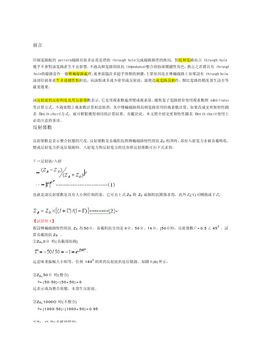
反射係數反射係數是表示整合狀態的尺度,反射係數是負載阻抗與傳輸線路特性阻抗Z0 相異時,部份入射電力未被負載吸收,變成反射電力折返信號源時,入射電力與反射電力的比亦即反射係數可由下式求得:Γ=反射波/入射也就是說反射係數是具有大小與位相的量,它可由上式Z R 與Z0 兩個阻抗關係求得,此外式(1)可轉換成下式:【試算例1】假設傳輸線路特性阻抗Z0 為50Ω,負載阻抗分別是0Ω、50Ω、1kΩ、j50Ω時,反射係數Г=0.5ㄥ450 ,試算負載阻抗Z R 。
①Z R=0Ω時(負載端短路)這意味著振幅大小相等,位相 1800相異的反射波折返信號源,如圖1(b)所示。
②Z R=50Ω時(整合)?=(50-50)/(50+50)=0這表示成為整合狀態,未發生反射波。
③Z R=1000O 時(不整合)?=(1000-50)/(1000+50)=0.95④Z R=∞O 時(負載端開放)這表示振幅大小相等,位相相等的反射波折返信號源,如圖1(a)所示。
工程电磁场第八版课后答案第10章
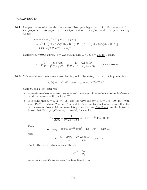
find:
p
a) C: Use Z0 = L/C, or
C
=
L Z02
=
5 ⇥ 10 (72)2
7
= 9.6 ⇥ 10
11 F/m = 96 pF/m
vp:
vp
=
p1 LC
=p (5 ⇥ 10
1 7)(9.6 ⇥ 10
= 1.44 ⇥ 108 m/s 11)
c) if f = 80 MHz:
p
2⇡ ⇥ 80 ⇥ 106
rs
s
Z0 =
Z= Y
R + j!L = G + j!C
17 + j2.1 ⇥ 102 75 ⇥ 10 6 + j2.4 ⇥ 10
2
= 93.6
j3.64 ⌦
10.2. A sinusoidal wave on a transmission line is specified by voltage and current in phasor form:
ej!t
=
2V0 Z0
sin(
z) sin(!t)
181
10.5. Two characteristics of a certain lossless transmission line are Z0 = 50 ⌦ and = 0+j0.2⇡ m 1
at f = 60 MHz.
p
p
a) Find L and C for the line: We have = 0.2⇡ = ! LC and Z0 = 50 = L/C. Thus
In phasor form, the forward and backward waves are:
2-2Smith Chart

12
Yin 1 1 (d ) 1 e j (d ) yin Y0 zin 1 (d ) 1 e j (d )
1 (d ) z in 1 (d )
•归一化的导纳可以由归一化阻抗在复Γ平面上旋转 180°得到,即导纳点是阻抗点关于原点的对称点。 •将Smith阻抗圆图旋转180°得到的圆图称为Smith导 纳圆图。 •归一化导纳和反射系数平面点存在一一对应关系。
28
2. 归一化负载阻抗
z L (30 j 60) / 50 0.6 j1.2
v p / f 0.5*3*108 / 2*109 7.5cm
d 2cm 0.267
29
开路线变换
采用开路线可以方便的得到纯感性和纯容性电抗。 传输线的特性阻抗为50Ω,工作在3GHz,相速度 为光速的77%,若要实现2.12pF的电容或5.3nH的 电感,所需开路短截线的长度。
2 2
1 半径 : x
1 圆 心 : r 1, i x
x的范围为<x<+, x可为负(容性),也可为正(感性)。 所有圆的中心都在过r =+1并垂直于实数轴r的线上。 x=时, 圆的半径为零,即r =+1和i =0的一个点。 x→0时, 圆的半径和圆的中心沿着垂直于实数轴(r)的线。
32
短路线变换
采用短路线可以方便的得到纯感性和纯容性电抗。 传输线的特性阻抗为50Ω,工作在3GHz,相速度 为光速的77%,若要实现2.12pF的电容或5.3nH的 电感,所需短路短截线的长度。
33
34
在Smith圆图上找到2.12pF的电容和5.3nH的电感 所对应的点,从短路点开始旋转至该两点,得到所 需线的长度。 实现2.12pF的电容需短路短截线0.425 λ,即 32.7mm 实现5.3nH的电感需短路短截线长0.176 λ,即 13.5mm
(完整word版)smith史密斯圆图(个人总结),推荐文档
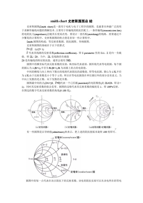
smith chart史密斯圆图总结史密斯圆图(Smith chart)是一款用于电机与电子工程学的圆图,是最著名和最广泛的用于求解传输线问题的图解技术。
主要用于传输线的阻抗匹配上。
一条传输线(transmission line)的电阻抗力(impedance)会随其长度而改变,要设计一套匹配(matching)的线路,需要通过不少繁复的计算程序,史密斯圆图的特点便是省却一些计算程序。
Smith圆图的构成:等反射系数圆、阻抗圆图、导纳圆图。
史密斯圆图的基础在于以下的算式Γ= (Z - 1)/(Z+ 1)Γ代表其线路的反射系数(reflection coefficient),即S-parameter里的S11,Z是归一负载值,即ZL / Z0。
当中,ZL是线路的负载值Z0是传输线的特征阻抗值,通常会使用50Ω。
圆图中的横坐标代表反射系数的实部,纵坐标代表虚部。
圆形线代表等电阻圆,每个圆的圆心为1/(R+1),半径为R/(R+1).R为该圆上的点的电阻值。
中间的横线与向上和向下散出的线则代表阻抗的虚数值,即等电抗圆,圆心为1/X,半径为1/X.由于反射系数是小于等于1的,所以在等电抗圆落在单位圆以外的部分没有意义。
当中向上发散的是正数,向下发散的是负数。
圆图最中间的点(Z=1+j0, Γ=0)代表一个已匹配(matched)的电阻数值(此ZL=Z0,即Z=1),同时其反射系数的值会是零。
圆图的边缘代表其反射系数的幅度是1,即100%反射。
在图边的数字代表反射系数的角度(0-180度)。
有一些圆图是以导纳值(admittance)来表示,把上述的阻抗值版本旋转180度即可。
圆图中的每一点代表在该点阻抗下的反射系数。
该电的阻抗实部可以从该电所在的等电阻圆读出,虚部可以从该点所在的等电抗圆读出。
同时,该点到原点的距离为反射系数的绝对值,到原点的角度为反射系数的相位。
由反射系数可以得到电压驻波比和回波损耗。
Smith Chart Utility_1

在原理图设计窗口中,执行菜单命令【Tools】-->【 Smith 】,弹出“SmartComponent Sync”对话框,选 择“Update simth Chart from SmartComponent ” 选项后,点击【 OK】按钮,弹出“Smith Chart Utility”对话框。
微波电路与系统
匹配电路设计
电子科技大学 贾宝富 博士
Smith Chart Utility界面介绍
工作参数设置 当前对应的原理图和SmartComponent
网络响应图
元件调用面板 匹配网络预览 做图区
参数提示区
集总参数电容电感匹配网络
集总参数匹配网络常用L型匹配网络
集总参数匹配网络设计实例
2、选中串联电感 3、在圆图中移动光标
1、选中负载端
添加并联电容
4、选中并联电容
5、移动光标到匹配点
5、点击此键,生 成电路原理图
看电路原理图
S参数仿真结果
自动生成L型匹配网络
去除源端锁定
去除锁定
输入源端匹配阻抗
4、在此对话框选 择匹配网络类型
1、选中源端 3、点击此键,自 动生成匹配网络
5、点击此键,生 成电路原理图
2、输入源阻抗的共轭
查看ADS电路原理图
6、点击此键,查 看电路原理图
S参数仿真结果
单支节匹配器
单支节阻抗匹配器也称阻抗调配器,是由串联传 输线段和并联支节构成,支节可以是短路支节也 可以是开路支节。 常见的单枝节阻抗匹配器的拓扑结构如下所示:
单支节阻抗匹配器
“Smith Chart Utility”对话框
由SmartComponent自动更新工作 频率、归一化阻抗和端口阻抗设置。
Smith Chart 史密斯圆图

Smith Chart Tutorial Part1To begin with we start with the definition of VSWR, which is the ratio of the reflected voltage over the incident voltage. The Reflection coefficient Γ is simply the complex (ie has phase) version of VSWR:-Define voltage standing wave ratio (VSWR)V V Voltage reflection coefficient - Complexmax min =+−V V V V 1212ΓV 1 e+j. β.lΓΓΓ =V V = V V At the load (l =0) ; =V V 212121e ee j j j −+−⇒.....βββlll2but this may be complex number if there is an instantaneous phase change which we’ll call (φ) on reflection.Phase Diagram0=L (a) ..... ∅()()DiagramCrank on d represente = V V=constant is L ith not vary w do V & V line lossless a For 0>L At .21221212.)0((L)l l βφβφφ−−−ΓΓΓ∴=Γ=Γj j j e e V V eCrank DiagramWe use a crack diagram as a way of representing the reflection coefficient phasor.()V = V VV V V V 12121e e e e e j j j j j +−+−−+∴=+=+........ββββφβl l ll l 1122ΓOALPAt the origin of argand diagram.OP = magnitude of total voltage/incidentvoltageβ.LOV Γ|As we saw previously the crack diagram with a circle drawn between points A & C is the beginnings of a Smith chart less the constant resistance and reactance circles/lines.VSWR =V V = 1+1- or =VSWR -1VSWR +1max min ΓΓΓ| V |V maxV minLLength OP’ -crank diagramvoltageincidentvAt B - 2. = -= 2.-= 4. = min mingφβπφβππλπφl l l min −∴From standing wave pattern measure VSWR ⇒ | Γ | @ l min ⇒ φ at load.SmithChart - Impedance (Z) or Admittance Y chart(1) Crank diagram + constant resistance & constant reactance circles.(2) Graphical solution to the equationcomplex= 11).2()(l βφ−ΓΓΓ−Γ+=j oin e Z Z(3) Smith Chart is a reflection coefficient diagramθ = φ-2.β.LSmith ChartOpen circuit x ⇒ ∞Short circuit v=0,x=0X = 0 ∴A is the matched point no reflectionOImpedance is plotted on the smith chart by first normalising to the characteristic impedance of the system (usually 50 ohms). In a 50 ohm system the centre of the smith chart is a pure 50 ohms.For example say we wanted to plot an impedance of 150 + j75ΩFirst normalise ie 150/50 = 3Ω ; 75/50 = 1.5Ω normalised impedance = 3+ j1.5ΩSo the real part of the impedance will lie somewhere along the r = 3 constant resistance circle ie:-Next we follow the constant reactance line at 0.75 to find the intersection of the r = 3 circle to get to our impedance point.3+j1.5Using the Smith Chart(1) Moving along the T.L = rotating around the Smith Chart.BACKWARDSFORWARDSFORWARDS (TO LOAD)BACKWARDS (FROM LOAD)(2) Constant |Γ| or VSWR circlesFor a lossless line |Γ| & VSWR do not vary with L.Γ| or VSWR|Γ| = 0 VSWR = 1|Γ| = 1∞1+1-Vmax = Z(max)Zo (real VSWR)Vmin =Z(min)ZoΓΓSS S ==1Vmin Vmax(3) Measure Lmin/λg ..... determines φ (at load).|V|LFORWARD by Lmin/λg takes us theload.λπlming−(4) Reading Z from chart also can get |Γ| & φ(5)Z Z o =+−11ΓΓAdmittance = Y/Y 0 =φY/Yo-|Γ|1 On a Smith chart point diametrically oppositeZ Z gives Y Y Note Y Y = G + j. Conductance Susceptance On admittance chart r circles g circles & x circles b circles.Note g =G Y and b = B Y o o0o o=→→1Z oβ(6) To transform an impedance along a T.L, rotate around the VSWR circle:-BACKWARDS by Lmin/λg takes us toZin.ZL/Zol/λg(7) Represent a series inductance on a smith chart.0.5Read values off the reactance scale0.20Therefore, assuming a frequency of say 1GHz the value of series inductance represented on the above Smith Chart is given by:-2.38nH E 1*2π0.3*50 2πN.XL 50 wrt 0.3 0.2 - 0.5 chart Smith from read )(X Reactance 9L L ===ΩΩ=Ω=fSimilarly for a series capacitor(8) Represent a series capacitance on a smith chart.Read values off the reactance scaleTherefore, assuming a frequency of say 1GHz the value of series capacitance represented on the above Smith Chart is given by:-ohms)50(usually factor g normalisin the is N Where 6.36pF 5.0*50*E 1*2π1.N.X 2π1 C 50 w.r.t 0.5 0.5 - 1.0 chart Smith from read )(X Reactance 9C C ===ΩΩ=Ω=fTo represent shunt reactance we need to plot admittance onto the Smith Chart. It is easiest to use a Smith chart with both impedance (usually in black) lines and admittance lines (usually in red) on the same chart. Or you can rotate the Smith chart 180 degrees.(9) Represent a shunt inductance on a smith chart.0.8Read values off the admittance scale0.2Therefore, assuming a frequency of say 1GHz the value of shunt inductance represented on the above Smith Chart is given by:-()ohms)50(usually factor on normaisati N 13.26nH6.0*E 1*2π50Y *2πNL 50 w.r.t 0.6mhos 0.2 - 0.8 chart Smith from read )(Y Admittance 9L L ====Ω=Ω=f(10) Represent a shunt capacitance on a smith chart.Read values off the admittance scale0.2Therefore, assuming a frequency of say 1GHz the value of shunt inductance represented on the above Smith Chart is given by:-()ohms)50(usually factor on normaisati N 2.5pF 50*E 1*2π0.8N *2πYC 50 w.r.t 0.8mhos 0.2 - 1.0 chart Smith from read )(Y Admittance 9C C ====Ω=Ω=f。
Smith圆图的Matlab实现及应用

分类号密级U D C 编号本科毕业论文(设计)题目Smith圆图的matlab实现及应用院(系)专业年级学生姓名学号指导教师二○○七年五月目录摘要 (1)关键字 (1)Abstract (1)Keywords (1)第1章前言 (2)第2章传输线阻抗匹配问题 (2)2.1阻抗匹配的重要性 (2)2.2 阻抗匹配的实现 (3)第3章 SMITH圆图的构成原理 (6)3.1反射系数圆 (6)3.2 阻抗圆图 (8)3.3 完成圆图 (11)3.4 导纳圆图 (12)第4章 SMITH圆图Matlab的实现 (13)4.1 圆图的绘制 (13)4.2 SMITH圆图软件设计的特点 (16)第5章 SMITH圆图的应用举例 (18)5.1 SMITH圆图的应用步骤 (18)5.2 根据负载阻抗求驻波比 (21)第6章总结 (22)参考文献 (23)致谢................................................... 错误!未定义书签。
摘要:基于smith圆图在进行阻抗匹配时具有方便、直观等特点,本文首先介绍了阻抗匹配的基础知识,在此基础上详细地阐述了smith圆图的构成原理,其中包括反射系数圆、阻抗圆图和导纳圆图,给出了各种圆图的具体推导过程。
接着提出了用matlab实现smith圆图的方法。
最后通过实例介绍了smith圆图的应用,归纳出了用matlab实现smith圆图具有省时、高效的特点,有推广的价值。
关键字:smith圆图matlab阻抗匹配Abstract:Based on the smith chart having the characteristic of convenient and intuitionistic in solving the problem of impedance matching, the elementary knowledge of impedance matching is introduced in the beginning of the paper, on this condition ,the paper describes constitution principle of the smith chart in detail and it includes the reflectance circle and the impedance circle diagram and the conductance circle diagram,and the concrete reasoning process of each kind of circle diagram is presented.Then the paper proposes realizable method of the smith chart with matlab. Finally,the paper introduces application of the smith chart,it is concluded that realization of the smith chart with matlab has the characteristic of highly effective and time-saving, has promoted value.Keywords:smith chart matlab impedance matching第1章前言工程中常采用smith圆图来分析传输线问题,传输线能引导电磁波沿一定的方向传输,为了提高传输线传输能量的效率,将输入的能量尽最大可能传给终端负载,需要保证传输线的终端的负载与其特性阻抗匹配,即传输线此时处于阻抗匹配状态。
- 1、下载文档前请自行甄别文档内容的完整性,平台不提供额外的编辑、内容补充、找答案等附加服务。
- 2、"仅部分预览"的文档,不可在线预览部分如存在完整性等问题,可反馈申请退款(可完整预览的文档不适用该条件!)。
- 3、如文档侵犯您的权益,请联系客服反馈,我们会尽快为您处理(人工客服工作时间:9:00-18:30)。
The Smith ChartContentsi.Introductionii.Waves on Ideal Transmission Linesiii.The Smith Chartiv.ReferencesIntroductionThis article deals with ideal transmission lines for electrical waves. If you would like a review of sinusoidal signals, phasors and transmission line equations, please read Backward Waves. We shall use the same notation here, except that the coordinate z that specifies location along a transmission line has z = 0 at the load instead of the source, and that we also use z as the normalized impedance Z/Z o, where Z o is the characteristic impedance of the line. To avoid confusion, -z is often represented by d.Our signals are sinusoidal waves of frequency f and wavelength λ, and fλ = v, the velocity of the waves. In free space, v = c = 2.9978 x 10⁸ m/s, approximately. In any material medium, v = c/n, where n is the index of refraction of the medium. Velocity on a transmission line is usually expressed by the velocity factor 1/n instead. When calculating wavelength on a transmission line, the velocity factor must be taken into account. Indeed, λ = c/nf = velocity factor x c/f. For theoretical work, the angular fre quency ω = 2πf, and the propagation constant k = 2π/λ are more convenient.For clarity, we shall consider only ideal lines in this article, those with no series resistance or shunt conductance. Actual lines approximate ideal lines rather closely, so this is not a serious limitation. Energy is conserved on an ideal line; the power out is the power in. The principal parameters of a line are its capacitance C and inductance L per unit length. The wave velocity is then v = 1/√(LC) and the characteristic impedance is Z o = √(L/C). These two parameters are generally quoted for any transmission line material.Coaxial cable RG-8/U has Z o= 53Ω and 1/n = 0.66. This velocity factor is typical of polyethyene (PE) insulation. RG-59/U, with Z o= 73Ω, has the same insulati on and velocity factor. RG-141/U, with polytetrafluoroetylene (PTFE) insulation, has Z o= 50Ω and 1/n =0.70. PE foam is mainly air, so RG-8/U(foam) has a velocity factor of 0.80 but about the same Z o= 50Ω. Coaxial cable has the great advantage that the f ields are totally enclosed. The molded 300Ω "twin-lead" has a velocity factor of 0.82. Parallel-wire lines in air have even larger velocity factors, usually about 0.95.A parallel-wire line with conductors of diameter d spaced a distance s betweeen centerlines has C = πε/cosh-1(s/d) and L = (μ/π)cosh-1(s/d). The product LC = με = 1/c2, so the idealvelocity factor is 1. The characteristic impedance is Z o = (cosh-1/π)√(μ/ε). √(μ/ε) = 377Ω, the wave impedance of free space. For d = 2mmand s = 20mm, Z o= 359Ω. The inverse hyperbolic cosines are calculateddirectly by the HP-48G, but can also be expressed in terms of naturallogarithms.Waves on Ideal Transmission LinesOn an ideal transmission line, there is generally a wave moving from source to load V'e-jkz, and a wave moving from load to source V"e jkz. The coefficients V' and V" are constants independent of z, since the line is lossless. The corresponding currents are (V'/Z o)e-jkz and-(V"/Z o)e jkz. All quantities are multiplied by the time factor e jωt, which is understood. The total voltage and current at any point are the sums of the contributions of the two waves.If the line is terminated at z = 0 with an impedance Z L, then this must be the ratio of the total voltage to the total current at that point, or Z L = Z o(V' + V")/(V' - V"). This condition establishes the ratio of V" to V'. Let us define the reflection coefficientρ(z) as the complex ratio (V"e jkz)/(V'e-jkz) = (V"/V')e2jkz. We then have z(0) = Z L/Z o = [1 + ρ(0)]/[1 - ρ(0)]. This equation can be inverted to give ρ(0) = [z(0) - 1]/[z(0) + 1]. The normalized load impedance determines the reflection coefficient at the load.At any other point on the line, a similar equation holds, but the complex reflection coefficient varies in a simple way. In fact, ρ(z) = ρ(0)e2jkz. That is, only the phase changes, while the magnitude remains constant. The magnitude will be represente d by ρ. In the usual case when the termination is resistive, ρ = [r(0) - 1]/[r(0) + 1]. As we move a distance d towards the source, ρ= ρe-2jkd. Therefore, the complex number ρ, represented as a vector, rotates clockwise through an angle (4π/λ)d. When d isλ/2, a half-wavelength, the vector has rotated through a complete circle.The maximum voltage on the line will be |V'| + |V"| and the minimum will be |V'| - |V"|. The ratio of the maximum to the minmum voltage is called the voltage standing wave ratio, VSWR, and there is an analogous definition for the current standing wave ratio. Clearly, maximum voltage corresponds to minimum current, and vice versa. The VSWR S = (1 +|ρ|)/(1 - |ρ|) in terms of the magnitude of the reflection coefficient. If |ρ| is zero, then S = 1 and the maximum voltage is constant along the line. If |ρ| = 1, then S is infinite, and there are points of zero voltage which correspond to points of maximum current, called nodes.The Smith ChartIf we let ρ = u + jv, this can be plotted in the (u,v) plane in the usual way of representing complex numbers. The normalized impedance, z = Z/Z o = [1 + ρ]/[1 - ρ] is a function of ρ, and so its real and imaginary parts, z = r + jx, can be expressed in terms of the real and imaginary parts of ρ = u + jv. If lines of r = constant and x = constant are drawn on thediagram, the result is called the Smith Chart, which is shown in the figure.This is a rather complex figure, but will repay careful study.First of all, the vertical and horizontal axes are v and u, the imaginary and realparts of ρ, which is normally represented in polar form. The outer circlecorresponds to ρ = 1 as well as to r = 0. The equation of the circle for a resistance r is [u - (r/r+1)]2 + v2 = (1/1+r)2, as can be seen by expressing z in terms of u and v, and finding the real part. The circle passing through points A and the origin B, of radius 1/2, corresponds to r = 1. Finally, point A corresponds to r = ∞.The normalized reactance, x, is also constant on circles which pass through A and have their centres on the v-axis. These circles are easily found to be (u - 1)2 + (v - 2/x)2 = (2/x)2. The parts of the circles for x = +1 and x = -1 are shown. Positive, or inductive, reactance is above the u-axis, while negative, or capacitive, is below. The u-axis corresponds to x = 0, or a z that is purely resistive.We note that point C corresponds to r = 0, or to a short at the load end of the line. Point B corresponds to r = 1, so the line is terminated in its characteristic resistance. At point A, r = ∞, or the line is open. Either point A or point C makes ρ = 1. As we proceed toward the source, the vector ρ rotates clockwise from whichever point describes the particular termination. While r remains zero, x goes through the complete range of values from +∞to -∞. This will be the reactance at any point along the line, and in particular, at the source. By changing the length of the line, we can present any desired reactive impedance to the source; at two points the reactance is zero, while the resistance is zero or infinity.If the line is terminated as at point B, then ρ = 0 (and doesn't go anywhere), while the impedance presented to the source is constant at z = 1, or Z = Z0. This important case is a matched line, and there is no reflection at the load end.A point P at an arbitrary location is shown also. It happens to lie on the r = 1 circle, so if it represents the termination of a line, the termination impedance has this real part, and some reactive part as well. This point determines a reflection coe fficient ρ and an angle θ which together determine the complex ρ. Any other point on the line is represented by some point on a circle of radius ρ with centre at B.This is important enough to be represented on a separate diagram. Let us assume that a line is terminated by a resistance at point A. For concreteness, suppose ρ = 0.6 and r = 0.2 at the point A. Suppose we are dealing with a 300Ω line at 200 MHz. The termination is then 0.2 x 300 = 60Ω. Suppose B represents the source end of the line. The angle θ is 135° (say), so 135° = 2(2π/λ)d = 720°d/λ. If the velocity coefficient is 0.82, the wavelength is 0.82 x c / 200MHz = 1.23 m. Now we can find the actual length of the line: d = (135/720)(1.23) = 23 cm. This end of the line is on the r = 1 circle, so the resistive component of the impedance is 300Ω. On an actual Smith Chart, we could also read off the reactance as well. Let's suppose it is x = 2. Then X = (2)(300) = 600Ω, inductive. Therefore, at point B, the impedance looking into the line is 300 + j600 Ω.The physical line is shown in the figure at the right. It is represented as constructed from300Ω plastic twinlead. The 60Ω resistor is not a standard value, but 56Ω would do about as well. Measuring the impedance at the input is a little more difficult, unless you have the very expensive insruments that can do it directly.Lines that are exactly a quarter-wavelength long have interesting properties. It is clear that the reflection coefficients at the two ends are simply negatives of each other, at the ends of a diameter in the Smith Chart. This means that if Z/Z o= (1 + ρ)/(1 - ρ) at one end, then Z'/Z o = (1 - ρ)/(1 + ρ) = Z o/Z at the other, or ZZ' = Z o2. This is called a quarter-wave transformer. Remember that when you design such a transformer, it will work as intended only at the design frequency, for only then is it a quarter-wave long.A quarter-wave line shorted at one end, as shown in the figure, is called a quarter-wave stub, and presents a very large impedance at its open end. Such stubs can be used to support a transmission line. Although there will be a DC path to ground, signal frequencies will be isolated. They will also act as pretty good bandpass filters, too, since only the signal current will not be shorted out.In this article, I have only presented the theory of the Smith Chart with a few examples. It has been used to solve problems of many standard types that arise in transmission line design. Of course, all the calculations can be done with a pocket calculator or computer, but the chart has the great advantage of giving a graphic picture of conditions that can give a deeper understanding and help in solving unusual problems. The interested reader should certainly examine an actual Smith Chart to appreciate how easy it is to use, and how quickly it provides answers.ReferencesS. Ramo, J. R. Whinnery and T. Van Duzer, Fields and Waves in Communication Electronics (New York: John Wiley & Sons, 1965). pp. 31-41. Fig. 1.20b is a Smith Chart that can be copied if no other source is available.Return to Tech IndexComposed by J. B. CalvertCreated 16 August 2003Last revised。