Numerical simulation of friction stir butt welding process for AA5083-H18 sheets
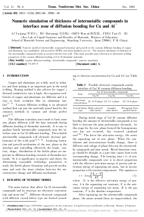
Numericsimulationofth_省略_sionbondingforC
bet ween the grains of intermet allic compounds and
base metal during t his course is not only on compo-
nent and atom arraying sty le, but also on the cryst al
T he diff usion t ransit ion zone t ends t o f orm some new phases dif ferent w ith the base mat erials during diffusion bonding of dissim ilar mat erials. It is easy to produce brit t le intermet allic compounds near the int erf ace zone in Cu/ Al diffusion bonding. T hese britt le intermet allic compounds w ill obviously decrease perf orm ance of the w eld joint [ 4, 6~ 8] . A nalyzing f orm at ion and g row t h mechanism of t he new phase in the interface and cont rolling effect ively the kinds, cont ent, shape, dist ribution of t he britt le phase are import ant in dif fusion bonding research of dissimilar m at erials. So it is signif icance in practice and t heory for det ermining reasonable technology paramet ers to st udy t he britt le phases format ion and g row th mechanism and seek t he inner relation betw een the m-i crost ruct ure change and diff usion mechanism.
元考试

有限元总复习1.What is simulation?模拟是通过一个系统描述其他物理系统或抽象系统的特定行为特征的过程。
(如可用一数据处理系统通过计算的方式再现物理现象)2.What is physical simulation?物理模拟是一种遵循和现实实际问题一样的物理现象和本质的模拟方法。
3.what is numerical simulation?数值模拟是一种遵循和现实世界相同规律的常微分方程和偏微分方程的模拟方法(有限元法就是虚拟实验过程)。
4.what is the finite element method?通过使用常微分方程和偏微分方程为边界问题提供一种近似解的数值计算方法。
5.Some advantages of FEM simulations ?a计算机模拟比真实实验方便经济b可以在设计过程中提前发现潜在问题c各种改进设计的方法可以快速的进行测试d可以显著减少真实实验次数6.The Procedure of the FEM (step 1 to step5)区域分散,单元分析,整体分析,数值求解,检查结果puter implementations of the FEM:a.预处理(建立有限元模型,加载,约束)b求解器(建立和求解系统过程)c后处理(整理并演示结果)8.Types of finite elementsa一维线性单元如杆单元,弹簧单元b二维平面单元如板单元壳单元c三维体单元如四面体4节点,四面体10节点9.Here [k]e﹛d﹜=﹛f﹜is the structure equation of an element,write the names ofthe [k]e﹛d﹜and﹛f﹜[k]e单位刚度矩阵﹛d﹜节点位移向量﹛f﹜节点力位移向量10.10 Here [u]= [N] ﹛d﹜is the displacement mode in an element,write the namesof the [u] [N] and﹛d﹜[u]位移向量[N] 形函数矩阵﹛d﹜节点位移向量11 .Single choice question(1)In rolling process of clad plate, there may beA. Reflective symmetry C. AxisymmetryB. Rotational symmetry D. Translational symmetry(2)One type of refinements in FE models is h-refinement, which means reduce the size ofthe element(3)One type of refinements in FE models is p-refinement, which meansA. enlarging the size of the element C. decreasing the order of the polynomialsB. reducing the size of the element D. increasing the order of the polynomialsh-refinement:——reduce the size of the element (“h” refers to the typical size of the elements);p-refinement:——Increase the order of the polynomials on an element (linear to quadratic, etc.; “p” refers to the highest order in a polynomial);(4)In 3-D analysis using MSC.AutoForge, rotational axis of a solid of revolution isA. y-axis of global coordinate system C. y-axis of local coordinate systemB. x- axis of global coordinate system D. x- axis of local coordinate system(5) For a discrete body, its degree of freedom isA. infinite C. constantB. finite D. unlimited(6) For a FE code such as MSC.AutoForge, materials properties are defined at the stageOf(7) For a FE code such as MSC.AutoForge, convergence testing are defined inA. loadcases C. postprocessingB. jobs D. preprocessing(8) For a LST element, the natural coordinates of node 4 are(9) For a quadratic quadrilateral element (Q8), the natural coordinates of node 6 areA. (1, 1) C. (1, -1)B. (-1, 0) D. (1, 0)(10) For a 8-node hexahedron the natural coordinates of node 6 are(11) On simulation of metal forming process using MSC.AutoForge, interface frictionbetween workpiece and tool is defined asA. a boundary condition C. an initial conditionB. a property of the contact body D. a contact table(12) Strip steel rolling process can be considered as(13) For a hexahedron element with 20 nodes, its displacement functions represented by polynomials may haveA. 8 items C. 16 itemsB. 10 items D. 20 items(14) FEM can simulate accurately REAL BEHAVIOR even though one of following aspects is not ensured:A. the physics and governing equations are sufficiently understoodB. the FEM model is correctC. the software is used properlyD. the symmetry properties are utilized(15) For a CST element, the stiffness matrix {k}e is a 6*6(16) For a LST element, the stiffness matrix {k}e is a 12*12(17) For a Q4 element, the stiffness matrix {k}e is a 8*812. Multiple-choice question(1) Some of the commercial FE codes are general purpose, such asA. MSC.MARC C. ANSYSB. MSC. AutoForgeD. ADINA(2) Some of the commercial FE codes are specific purpose, including(3) Spring elements are not suitable forA. stiffness analysis C. temperature analysisB. stress analysis of the spring itself D. strain analysis of the spring itselfE. buckle analysis(4) Spring element can have(5) Most structural analysis problems can be treated as linear static problems, based onsome of the following assumptionsA. Small deformations C. Uniformly distributed loadsB. Elastic materials D. Static loads(6) In general a stiffness matrix of an element is(7) About CST Element the incorrect expressions of the following areA. Avoid use in areas where the strain gradient is smallB. Use in mesh transition areas (fine mesh to coarse mesh).C. Using in stress concentration or other crucial areas in the structure, such as edges of holes and corners.D. Suitable for composite materialsE. Recommended for quick and preliminary FE analysis of 2-D problems(8) Plastic deformation problems are usually related to combined nonlinearities including(9) Quadratic elements are preferred for stress analysis, because ofA. their high accuracyB. the flexibility in modeling complex geometryC. little effort for calculationsD. easy to modeling(10) In FEM simulation avoid elements with(11) In FEA the aim of applying symmetry of a structure isA. to reduce the size of the problems C. to simplify the modeling taskB. to make it easy to check the results D. to make it easy to apply BC’s(12) Types of errors in FEA are as followsA. Modeling Error C. Random ErrorB. Discretization Error D. Numerical Error(13) In thermo-mechanical analysis, types of boundary conditions can beA. load C. heat transferB. displacement D. velocity(14) In the following properties which one is incorrect for the stiffness matrix of anelement?A. square C. symmetryB. banded D. nonsingular(15) For a symmetrical problem, each element may be a ring with a cross-section of(16) For a model of axisymmetry problem, each element may be a ring with a cross-section ofA. square C. triangleB. rectangle D. quadrilateral13. Explain the meanings of terms as follows.(1)DOF : Degree of Freedom, 节点自由度:只一个节点的位移矢量的分量的个数。
精编汽车焊装英文词汇

序号英文全称缩写中文全称A1AC Gun工频焊钳2Accuracy /ˈækjurəsi/精度3acquisition of signal信号采集4aging /ˈeidʒiŋ/时效处理5air压缩空气6air hoist /hɔist /气动葫芦7air pipe气管8air pressure regulator-filter空气过滤减压阀9air spanner气动扳手10alternator /ˈɔːltəneitə/交流发电机11alternator bracket发电机支架12anneal /əˈniːl/退火13Anti-lock Brake System ABS防抱死刹车系统14Arc Welding弧焊15Arm电极臂16assembly drawing装配图17asynchronous /eiˋsiŋkrənəs/ motor异步电动机18ATC自动换枪装置19Auto Gun自动焊钳20automatic feed自动喂料21automatic mechanical transmission AMT自动换档机械式变速器22automatic transmission /trænzˈmiʃən/AT自动变速箱B23ball bearing球轴承24bar /bɑː/棒材25Bearing轴承26belt皮带27billet /ˈbilit /方钢28black oxide coating发黑/发蓝29blank /blæŋk/坯料,半成品30Blanking /ˈblæŋkiŋ/下料31Body In White BIW白车身32BODY INSPECTION FIXTURE车身综合检具33body respot line车身补焊线34Body Shop车身车间35boring/ˈbɔ:riŋ/镗削36breaker /ˈbreikə/断电器37Brittleness脆性38BURR /bɜː/毛刺C39C Type Welding Gun C型焊枪40calibration /ˌkæliˈbreiʆən/校准41capacity /kəˈpæsiti/容量,规格42carbon-dioxide arc welding; CO2arc welding二氧化碳气体保护电弧焊43case hardening表面硬化44casting铸造45catalog /ˈkætəlɒg/库46centering table 对中台47chain 链条48chain gear链轮49chamfer倒角50chromium /ˈkrəʊmiəm/铬51chuck吸盘52clamping force夹紧力53clearance fit间隙配合54commission /kəˈmiʆən/现场调试55Computer Aided Design CAD计算机辅助设计56Computer Aided Process Planning CAPP计算机辅助工艺过程57Computer Numerical Control CNC计算机数控加工58Concurrent /kənˈkʌrənt/EngineeringCE并行工程59configuration /kənˌfigəˈreiʆən/组态60control cabinet /ˈkæbinit/控制柜61control panel控制屏,控制盘62control system操纵系统63converter /kənˈvɜːtə/变频器64conveyor /kənˈveɪə/输送机65conveyor belt皮带机66cooperation/kəuˌɔpəˈreiʃən/合作67coordinate frame of car车身坐标系68corrosion/kəˈrəʊʒən/腐蚀69cotter /ˈkɔtə(r)/开口销70counter weight配重71crack /kræk/裂纹72current gauge电流测试仪73cycle time节拍74cylinder /ˈsilində/气缸D75damped glue膨胀减振胶76data acquisition /ækwiˈziʃ(ə)n/数据采集77data preprocessing数据预处理78data processing数据处理79data processor数据处理器80debug程序调试81debur去毛刺82definition /ˌdefiˈniʆən/定义83deflection /offset偏移84delta三角形85d elay /ˈdiːlei/延时86depalletizer/diˈpæliˌtaizə/拆垛小车87die/dai/冲模88die changer模具交换器89digital model数模90Digital Signal Processing DSP数字信号处理91display /diˈsplei/显示92dowel/daʊəl/ pin定位销93drilling/ˈdriliŋ/钻削94duty ratio负荷比E95electric hoist /hɔist/电动葫芦96electric welding machine; electricwelder电焊机97electrically operated valve电控阀98electrocladding /plating电镀99electrode holder焊钳100electromagnetic /ilektrəʊˈmæɡnitik/compatibility /kəmˌpætiˈbiliti/EMC电磁兼容性101engine /ˈendʒin/发动机102epoxy resin glue for hemming环氧折边胶F103fault diagnosis故障诊断feedback /ˈfiːdbæk/反馈104fender /ˈfendə/防护板、翼子板105106field bus现场总线107fillet /ˈfilit/角焊缝fillet welding角焊108flange /flændʒ/法兰109Flexible Body Line FBL柔性车身线110111flow chart流程图112forging锻造113fork truck叉车frame/coordination坐标114friction stir welding搅拌摩擦焊115G116gantry /ˈgæntri/龙门架117gap /gæp/间隙118gauge /geidʒ/型板119gears /giə:s/档位120Geo-Gripper定位抓具121Geometry /dʒiˈɒmitri/GEO几何122Geo-spot定位焊点123gluing/glu:iŋ/涂胶124Gluing Robot涂胶机器人125governor /ˈgʌvənə/调速器126grinder /ˈgraində/磨光机127grinding /ˈgraindiŋ/磨削128gripper抓具129groove /gruːv/坡口130ground地线;接地131gun hanger焊钳吊钩132gun switch焊钳开关H133hand gun手动焊钳handling robot取件机器人;搬运机器人134135hanger/ˈhæŋə/吊具hardening and tempering调质136heat/thermal treatment热处理137138hemming滚边139hemming bed胎模hemming die包边模具140hemming press包边压力机141142hemming tool滚边工具horizontal /ˌhɒriˈzɒntl/水平143144hot-melt adhesive热熔胶145human ergonomics/ˏɜːgəˈnɔmɪks/人机工程human-machine interface HMI人机界面146147hydraulic /haɪˈdrɔːlik/液压的148hydraulic absorber液压缓冲器I149induction machine感应式电机150inertia惯性;惯量151information of weld point焊点信息152inner dimension内部尺寸153inspection fixture I/F检具154interference /ˌintəˈfiərəns/干涉155interference fit过盈配合156invoice发票157isolating transformer隔离变压器J158jog /dʒɒg /点动(机器人等)159joint /dʒɔint/运动关节K160kinematic /kɪniˈmætɪk/运动学的, 运动学上的L161laser welding/ laser beam welding激光焊162layout规划,布局图163leg/ fillet weld leg焊脚164lifter升降机165light curtain /ˈkə:tən/安全光栅166linear unit直线单元167location位置168location pin定位销169lubricating oil润滑油M170magnet/ˈmægnit/磁铁171main reducer主减速器172man-machine coordination人机协调173mass production大批量生产174Master Control Point MCP主要控制点175master control point chart MCP图176Master Control Section MCS主控截面177master station主站178mechanical transmission MT机械式变速箱179mechanism /ˈmekənizəm/机构180Metal Active Gas welding MAG金属极(熔化极)活性性气体保护焊181Metal Inert Gas welding MIG 金属极(熔化极)惰性气体保护焊182MF Gun中频焊枪183milling/ˈmiliŋ/铣削184modify /ˈmɒdifai/更改185mounting plate安装面186multiple spot welding多点焊N187normalizing正火188nozzle /ˈnɒzəl/喷嘴O189Off-line Programming OLP离线编程190On-Board Diagnostics OBD在线检测191open大开192operating mechanism操作机构193orientation /ˌɔːriənˈteiʆən/方位194over voltage relay过电压继电器P195pallet /ˈpælit /物料架,小车托盘196parameter /pəˈræmitə/参数197part drawing零件图198patent/ˈpeɪtnt, ˈpætnt/专利199pay roll工资单200peak time峰值时间201performance characteristic工作特性202peripheral外围设备203pillar /ˈpilə/立柱204pipe joint管接头205piston/ˈpɪstən/活塞206pitch节距207planing /ˈpleiniŋ/刨削208planning规划209pneumatic /njuːˈmætik/气动210pneumatically /njuːˈmætikəli/drived slider气动滑台211position位置212positioner变位机213postweld heat treatment/postheattreatment焊后热处理214press压力机215Press Line冲压线216pressing robot冲压机器人217process /ˈprəʊses/工序;工艺(强调过程)218profile轮廓219project /ˈprɒdʒekt /工程、项目、投影220projection welding凸焊221property /ˈprɒpəti/属性Q222quenching /ˈkwentʃiŋ/淬火R223rack /ræk/支架;齿条224rail /reil/轨道;横梁225reachable可达226reducing valve减压阀227Regulator Interface Panel RIP水气排228Reinforce glue补强胶229reinforcement /ˌriːinˈfɔːsmənt/加强230reliability /riˌlaiəˈbiliti/可靠性231rid棱;加强肋232rigidity /riˈdʒidəti/刚度233robot programming language机器人编程语言234robot simulation机器人仿真235robot teaching机器人示教236roller /ˈrəulə/滚头237rope hemming水滴包边S238sandblast /ˈsændblɑːst/喷砂239Sealer Pump涂胶泵240seam /siːm/接缝241section型材,断面242security /siˈkjuəriti/lock安全锁243self-lubricant/self ˈlu:brikənt/ Bearing润滑轴承244semiopen小开245sensor /ˈsensə/传感器246Servo Gun伺服焊钳247servo motor伺服电机248short-circuiting,bridge短路249shuttle /ˈʆʌtl/往复输送250simulated interrupt仿真中断251Simulation仿真252simultaneous Engineering SE同步工程253solenoid /ˈsəulinɔid/valve/vælv/电磁阀254spatter /ˈspætə/飞溅255spherical /ˈsferɪk(ə)l / roller万向球256Spot Welding Sealants点焊密封胶257spot welding; resistance spotwelding点焊258spring /spriŋ/弹簧259squeeze挤压260stability /stəˈbiliti/稳定性261stand /stænd/换枪架262station /ˈsteiʆən/工位263steel rail 钢轨264strategic/strəˈtiːdʒɪk/战略的265strength /streŋθ, strenθ/强度266stud /stʌd/welding植焊267summary /ˈsʌməri/摘要268surface roughness表面粗糙度269symmetrical对称的;平衡的T270tapping攻丝271task /tɑːsk/任务272technique /tekˈniːk /工艺(强调技术手段)273temperature control device温度控制元件274tensioning/ˈtenʃəniŋ/wheel张紧轮275terminal电极,终端(点);接线柱276test signal测试信号277thread/θred/螺纹278through /θru:/直通279throughput产量;生产能力280TIMER CONTROLLER T/C焊接控制箱281TIP电极帽282tip dresser修磨器283tip; contact tube导电咀284tool changer换枪装置285torch /tɔːtʆ/焊炬;弧焊焊枪286torque /tɔ:k/扭矩;转矩287touch screen;touch panel触摸屏288TRANSFORMER T/R焊接变压器289transition fit过渡配合290Trolly滑车291Tungsten Inert Gas/Gas TungstenArc WeldingTIG/GTAW钨极(非熔化极)惰性气体保护焊;钨极氩弧焊292Turn table回转台293turning /ˈtə:niŋ/车削294twist drill麻花钻295two-way valve二通阀U296unmanned无人化的V297valve /vælv/阀298velocity transducer速度传感器299vertical /ˈvɜːtikəl/垂直300virtual manufacturing虚拟制造W301washer垫片302wear and tear磨损303weldability焊接性304welding controller焊接控制器305welding current downslope time焊接电流衰减时间306welding cycle焊接循环307welding gun焊枪308welding machine; welder焊机309welding power source焊接电源310welding process焊接工艺311Welding Robot焊接机器人312welding spot焊点313welding technique焊接技术314wire cutting电火花线切割315worm蜗杆316worm gear=worm wheel蜗轮X317X Type Welding Gun X型焊枪BIW相关词汇318ASSEMBLY ASSY总成319BODY BUILD B/B总成320BODY COMPLETE B/C总成321BODY FLOOR B/F地板322BODY IN WHITE BIW白车身323BODY SIDE B/S侧围324BRACKET BRKT支架325CENTER CTR中央通道326COMPLETE COMPLT组件;总成327DOOR DR门328ENGINE ENG发动机329EXTENTION EXTN延伸330FLOOR FLR地板331FRONT FR;FRT前部332HEAD LAMP H/LAMP前大灯333INNER INR内部的334LEFT HAND LH左侧335LOWER LWR下部336MEMBER MBR纵梁337OUTER OTR外部338PANEL PNL面板339RADIATOR RAD水箱340RADIATOR SUPPORT R/SUPT水箱横梁341REAR RR后部342REINFORCEMENT REINF加强343RIGHT HAND RH右侧344ROOF RF顶盖345SIDE OUTER S/OTR外侧346SIDE SILL S/SILL侧裙边347SUB ASSEMBLY SUB ASSY分总成348SUN ROOF S/RF天窗349SUPPORT SUPT支撑350UNDERBODY UB地板351UPPER UPR上部352intake pipe进气管353fire wall,dash panel前围板354rear wall后围板355tailgate后背板356fender翼子板;挡泥板357fuel filler加油口358front pillar,A-pillar A柱359center pillar,B-pillar B柱360rear pillar,C-pillar C柱361rail横梁362hinge铰链363guide rail导轨。
NUMERICAL SIMULATION OF FRICTION STIR WELDING PROCESS

NUMERICAL SIMULATION OF FRICTION STIR WELDING PROCESSDongun Kim 1, Harsha Badarinarayan 2, Ill Ryu 1, Ji Hoon Kim 3, Chongmin Kim 4,Kazutaka Okamoto 5, R. H. Wagoner 3, Kwansoo Chung 1,*1Department of Material Science and Engineering, Seoul National University2Research and Development Division, Hitachi America Ltd.3Department of Materials Science and Engineering, The Ohio State University 4Materials and Process Lab., R&D Center & NAO Planning, General Motors Corporation5Hitachi Research Laboratory, Hitachi Ltd.ABSTRACT: Thermo-mechanical simulations of the friction stir butt welding and friction stir spot welding processes were performed for AA5083-H18 sheets, utilizing commercial FVM codes which are based on the Eulerian formulation. For the friction stir butt welding process, the computational fluid dynamics code, STAR-CCM+, was utilized under the steady state condition. Temperature and strain rate histories along the material flow were calculated and simulated temperature distributions (profiles and peak values) were compared with experiments for verification. It was found that by including proper thermal properties of the backing plate (anvil) the accuracy of the simulation results increased significantly. For the friction stir spot welding process, the computational fluid dynamics code, STAR-CD, was utilized under the unsteady condition to understand the effect of pin geometry on material flow and weld strength.KEYWORDS: Friction stir butt welding, Friction stir spot welding, Thermo-mechanical Simulation, AA5083-H181 INTRODUCTIONIn this report, simulations of the friction stir butt welding (FSBW) as well as friction stir spot welding (FSSW) processes were performed utilizing Eulerian Computational Fluid Dynamics codes, STAR-CCM+ [1]and STAR-CD [2]. Thermo-mechanical simulations were carried out for AA5083-H18 as a coupled analysis along with the user subroutine to define temperaturedependent material properties. As for the FSBW case, the process, consisting of plunging, short dwell, longlinear welding and retracting steps, was simplified as asteady state process wherein the process achieves anequilibrium operating temperature in a relatively shorttime [3]. As for the FSSW case, the process consists of plunging, short dwelling and retracting steps. Unlike the FSBW process, the FSSW cannot be considered as a steady state process wherein the whole welding process is conducted in a short time as well as consists of a shortdwelling step. Simulations were directly verified for temperature history in the case of FSBW but indirectlyfor spot weld strength in the FSSW case. ____________________* Corresponding author: Address: 33-214, San 56-1, Shillim-Dong, Gwanak-Gu, Seoul 151-742, KoreaPhone: 82-2-880-7189, Fax: 82-2-885-1748 and Email: kchung@snu.ac.kr2 THEORYIn order to calculate the temperature distribution and plastic deformation during FSW Process, continuity and momentum equation as well as energy equation aresolved with temperature dependent or temperature and strain rate dependent material properties. Theconstitutive law (for the mechanical strain) is assumed rate-insensitive and incompressible rigid-perfect Misesplastic using the normality rule, 3222and and σεμεσμσε∂===∂==S S D D S S = (1)where and are the rate of deformation tensor and the deviatoric stress tensor, and D S σ, ε and μ are the Mises effective yield stress, effective strain rate and the viscosity. The yield stress is temperature dependent property and the viscosity is temperature and strain rate dependent property, given by eq. (2) 3σμε= (2)a baffle heat transfer boundary condition was applied, in which the relation between the heat flow rate across thecontact boundary with an area A is given byniii n dT Tq kA R dn Rk AΔΔ=−≈−=∑(3)DOI 10.1007/s12289-009-0459-z © Springer/ESAFORM 2009Int J Mater Form (2009) Vol. 2 Suppl 1:383–386where and are the thermal conductivity and thickness, respectively, of the i-th layer comprising the contact boundary and R is a representative thermal resistance for the area A (here, the n-direction is normal to the boundary surface). Eq. (3) is derived under the condition that the heat flow rate is maintained for each layer comprising the contact boundary. i k i n Δ3 EXPERIMENTS3.1 FSBWFSBW was performed on AA5083-H18 sheets by using a CNC controlled 3-D FSW system “Hitachi GR-3DM10T” with 11 KW spindle servomotor, as shown in Figure 1 [4].Figure 1: CNC controlled 3-D FSW system “Hitachi GR-3DM10T” with 11 KW spindle servomotor and description for the welding process.The anvil upon which the work-piece is laid for welding was made of a low carbon steel 1020, while the tool was made of tool steel H13 with the shoulder and pin diameters of 10 mm and 4 mm, respectively. The shoulder had a concave profile which acts as an escape volume for the material displaced by the pin, while preventing the material from extruding out of the sides of the shoulder and maintaining downward pressure. The pin is right-hand threaded. The pin length is slightly less than the thickness of work-pieces, with 1.34 mm for AA5083-H18 (sheet thickness of 1.64 mm). The welding tool was tilted at an angle of 3 degree from the normal direction of the work sheets towards the trailing side of the tool. Three welding conditions were tried out: 1,000 rpm/100 mm/min, 1,000 rpm/300 mm/min and 1,500 rpm/150 mm/min (=rotational/linear translational speed).Figure 2: Schematic illustration of thermocouple placement.As shown in Figure 2, for measuring temperature in the regions near the top surface, three small channels, into which sheathed K-type thermocouples were placed, were machined from the sheet bottom surface up into the sheet by 1.04 mm. The tip of the thermocouples was located 2 mm, 5 mm, and 8 mm away from the weld seam line, respectively. All the temperature measurements were made on the advancing side as well as retreating side of welds.3.2 FSSWFSSW was performed on AA5083-H18 (sheet thickness of 1.64mm-upper one and 1.24 mm-lower one) sheets by using a CNC controlled 3-D Linear FSW system “HitSpin type GR3DC5T” with 7.5 KW spindle servomotor, as shown in Figure 3.Figure 3: CNC controlled 3-D linear FSW system ‘HitSpintype GR3DC5T’ and welding jig with a coupon in a cross-tension configuration.Welds were made in a cross-tension configuration with coupon dimensions being 150 mm x 50 mm, as shown in Figure 3 with the jig used for welding [5]. Since the purpose of this study was to evaluate the effect of tool geometry on static strength, the weld parameters were fixed as follows: the tool rotation speed was 1,500 rpm, while the plunge and retract speed was 20 mm/min and the dwell time was 2 seconds.Cross sectional macro- and micro-structures of welds were examined by using an optical microscope for AA5083-H18 sheet. The specimens were also tested for weld strength on an Instron screw driven test machine at a constant crosshead speed of 5mm/min. [6]4 SIMULATIONS4.1 FSBWThe thermo-mechanical simulation of the FSBW process for AA5083-H18 was performed using the CFD code, STAR-CCM+ [1]. Dimensions of the model are shown in Figure 4. The work-piece is 200 mm x 600 mm x 1.64 mm in thickness which lies on an anvil with similar dimensions but with the thickness of 10mm. The radii of the pin and the tool shoulder were 2 mm and 5 mm, respectively. The pin length was 1.34 mm from the tool shoulder edge and the plunging depth of the tool shoulder edge was 0.2 mm. The concavity of the shoulder was 10 degrees and the tool was tilted at an angle of 3 degrees in the trailing direction of the weld line.Figure 4: Dimensions of the thermo–mechanical model: topview and section view of the tool (in mm).The rate-insensitive and incompressible rigid-perfect Mises plastic property was applied for the work-piece as described in Section 2. Temperature dependent yield384stresses for AA5083-H18 were used in this work, as shown in Table 1. As for thermal properties, only the room temperature data was available for AA5083-H18 and their temperature dependent properties were not available. Therefore, assumed temperature dependent properties were obtained from those of AA5052-H32 [7] by proportionally modifying the values considering the ratios at room temperature values of the two materials, as shown in Table 2. And constant thermal properties were implemented for anvil material with Low Carbon Steel 1020, as shown in Table 3 [8].Table 1: Temperature dependent yield stressTemp.(o C) Y.S.(MPa)20 440 100 437 200 364 300 181 400 61 440 50 540 40 570 0Table 2: Temperature dependent thermal conductivity, specificheat and density of AA5083-H18Temp.(o C) Conductivity (W/m o C) Specific Heat (J/Kg o C) Density (Kg/m 3)-20 112.5 924.1 2673.980 122.7 984.2 2642.7180 131.6 1039.6 2629.4280 142.3 1081.2 2611.5380 152.5 1136.6 2589.3480 159.5 1178.2 2567.0580 177.2 1261.42549.2Table 3: Material properties of Low Carbon Steel 1020 atroom temperatureConductivity(W/m o C) Specific Heat (J/Kg o C) Density (Kg/m 3)51.9 486.0 7,850.0As for the heat equation, the convective heat transfer coefficient of 30 W/m 2°C was used for the top and sides of the work–piece, which is typical for natural convection heat transfer between aluminum and air [9]. The baffle heat transfer boundary condition was placed with one layer each for the work-piece and the anvil. Also, the convective heat transfer coefficient of 35 W/m 2°C was used for the sides of the anvil which is typical for natural convection heat transfer between steel and air [10]. At the bottom of the anvil, the coefficient was assumed 200 W/m 2°C. Heat transfer at the interface between the tool and the work-piece was also ignored with the vanishing temperature gradient at the boundary.4.2 FSSWThe thermo-mechanical simulation of the FSSW process for AA5083-H18 was performed using the CFD code, STAR-CD [2]. The FSSW process consists of tool plunging, a short dwelling and tool retracting steps. But, only the 2 second dwelling step was simulated in which the rotating tool was plunged into the work-piece in a lap configuration. Two types of pins were considered: cylindrical and triangular pins with concaved shoulders. Unlike the FSBW, the FSSW was considered as an unsteady state process. The cylindrical and triangularpins both have 10 degree concave shoulders. The pinradius was 2.5 mm and the shoulder radius was 6 mm, while the pin length was 1.6 mm from the shoulder edge and the plunge depth of the shoulder was 0.2mm. The diameter of the circle inscribed by the triangular pin was the same as the diameter of the cylindrical pin. The model description and dimensions are shown in Figure 5 with 2.88mm thickness (two work-pieces in a lab configuration were considered as one piece) with the work-piece radius of 50mm.Figure 5: Top view for cylindrical pin and triangular pin(upper), and model dimension (lower).The convective heat transfer coefficient of 30 W/m 2°C was used for the top and sides of the work–piece [9]. At the bottom of the work-piece, the convective heat transfer coefficient was assumed to be 2,000 W/m 2°C just below the tool considering that heat transfer between two contacting surfaces increases when the pressure between them increases under the tool [11]. For the remaining bottom surface, the coefficient was assumed 200 W/m 2°C.5 Results5.1 FSBWIn order to verify the numerical simulation results, the simulated temperature peak values were compared with experimental results [4] that were obtained using thermocouples at various locations along the weld path, as shown in Table 4 and Figures 6~10. The simulation results matched very closely with experiments.Table 4: Result summaries showing experimental andsimulation result for each case.Advancing Side Retreating Side 2mm 5mm 8mm 2mm 5mm 8mm1000rpm 100mm/min Experiment 525 420 300 480 400300Simulation 525 448 276 516 4272661000rpm 300mm/min Experiment 460 400 205 ···Simulation 467 401 223 459 3772061500rpm 150mm/min Experiment 530 450 267 ···Simulation 541 444 266 535 430257(a) (b) (c)Figure 6: Computed and experimental temperature history atlocations away from the weld center along the width on the advancing side385(a) (b)(c) Figure 7: Temperature profile at the top surface for each welding conditions(a) (b)(c) Figure 8: Temperature cross section profile near the tool for each welding conditions(a) (b)(c) Figure 9: Material flow with strain rate history for each welding conditions(a) (b)(c) Figure 10: Material flow with temperature history for (a) 1000rpm and 100mm/min, (b) 1000rpm and 300mm/minand (c) 1500rpm and 150mm/min (in °C)5.2FSSWTemperature profiles at the top surface as well as any cross section surface of sheets for the cylindrical and triangular pins were calculated at various moments. Also, material flow patterns were simulated at various instances. For the cylindrical pin, materials near the tool did not move that much along the radial direction. However, for the triangular pin, materials near the pin boundary showed significant in and out motion along the radial direction, since the boundary of the triangular pin moved in and out along the radial direction during the tool rotation. Note that heat generation of the cylindrical and triangular pins was similar, only the material flow pattern was different which then caused the static weld strength to be different. The weld strength for the concave triangular pin was almost twice as that of the concave cylindrical pin. The triangular pin geometry yielded higher weld strength compared to the cylindrical pin, since the material flow pattern affected the hook formation near the pin, as shown in figure 11 [6].(a) cylindrical pin (1,800N) (b)triangular pin (3,600N) Figure 11: Sectional macrographs in the cross-tension test6CONCLUSIONSThe FSBW process was solved under the steady state condition and simulated temperature results matched with experiments very closely, while nobody has achieved such an agreement of the numerical results with experiments. Above results from the simulation can be a good control group to study welds performances. In particular, the effective strain results as well as the temperature history of welds may play an important role in the decision of the grain size after welding as well as the AGG (abnormal grain growth) phenomenon, where one grain grows at a much greater rate than its neighbours, after PWHT (post weld heat treatment). As for the FSSW, simulation was conducted under the unsteady state condition to understand the tool geometry effect on weld strength. Simulated material flow pattern was discussed to explain the hook formation near the pin boundary since the hook formation is a key geometric characteristic of the weld strength. ACKNOWLEDGEMENTThe authors of this paper would like to thank the Korea Science and Engineering Foundation (KOSEF) for sponsoring this research through the SRC/ERC Program of MOST/KOSEF (R11-2005-065). REFERENCES[1]CD-Adacpco, 2007. STAR-CCM+ 2.10.017.[2]CD-Adapco, 2005. STAR-CD 3.26[3]Badarinarayan, H., 2007. APL Effect of ToolThermal Expansion and Durability in Friction StirSpot Welding, Hitachi America Ltd., Internal Report [4]Okamoto, K., Hirano, S., Inagaki, M. and Odakura,T., 2004. Friction Stir Welding of Automotive AlloySheets for Tailor Welded Blank, Hitachi Ltd.,Internal Report[5]Badarinarayan, H., Yang, Q. and Hunt, F., 2008a.Effect of Tool Geometry and Pin Length on FailureMode and Static Strength of Friction Stir SpotWelds, SAE World Congress & Exhibition, SAE,Detroit, MI, USA (Paper #2008-01-0147)[6]Badarinarayan, H., Yang, Q. and Zhu, S., 2008b.Effect of Tool Geometry on Static Strength ofFriction Stir Spot Welded Aluminum Alloy,International Journal of Machine Tools &Manufacture, doi:10.1016/j.ijmachtools.2008.09.004 [7]Zhu, X.K. and Chao, Y.J., 2002. Effects ofTemperature-dependent Material Properties onWelding Simulation, Computers & Structures, Vol.80, pp. 967-976[8]Callister Jr., W. D., 2003. Materials Science andEngineering: an Introduction 6th Ed., pp.737~758 [9]Chao, Y.J., Qi, X. and Tang, W., 2003. HeatTransfer in Friction Stir Welding-Experimental andNumerical Studies, Transactions of the ASME Vol.125, p.138[10]Totten, G. E., 2007. Steel Heat Treatment Handbook2nd Ed., CRC Press, p. 567[11]Hyoe, T., Colegrove, P. A. and Shercliff, H. R.,2003. Thermal and Microstructure Modelling inThick Plate Aluminium Alloy 7075 Friction StirWelds, Proceeding of TMS Spring Meeting, FrictionStir Welding II, TMS, San Diego, CA, USA386。
Vorton Formation
a rXiv:h ep-ph/984378v123Apr1998Vorton FormationC.J.A.P.Martins ∗and E.P.S.Shellard †Department of Applied Mathematics and Theoretical Physics University of Cambridge Silver Street,Cambridge CB39EW,U.K.In this paper we present the first analytic model for vorton forma-tion.We start by deriving the microscopic string equations of motion in Witten’s superconducting model,and show that in the relevant chiral limit these coincide with the ones obtained from the supersonic elastic models of Carter and Peter.We then numerically study a number of solutions of these equations of motion and thereby suggest criteria for deciding whether a given superconducting loop configuration can form a vorton.Finally,using a recently developed model for the evolution of currents in superconducting strings we conjecture,by comparison with these criteria,that string networks formed at the GUT phase transition should produce no vortons.On the other hand,a network formed at the electroweak scale can produce vortons accounting for up to 6%of the critical density.Some consequences of our results are discussed.I.INTRODUCTION As first pointed out by Witten [1],cosmic strings can in some circumstances (typically when the electromagnetic gauge invariance is broken inside the string)behave as ‘superconducting wires’carrying large currents and charges—up to the order of the string mass scale in appropriate units.The charge carriers can be either bosons or fermions (see [2]for a review).The former type occurs when it becomes energetically favourable for a charged Higgs field to have a non-zero vacuum expectation value in the string core;the latter happens when fermions couple to the string fields creating fermion zero modes.It is well known that arbitrarily large currents are not allowed—there is a criticalvalue beyond which the current saturates.In other words,for large enough wind-ing number per unit length,the superconducting condensate is quenched down,suppressing the current flow.Also,the current can decay by magnetic flux-line tun-nelling;this can be used to impose constraints on allowed particle physics models.If superconducting strings carry currents,they must also carry charges of similar magnitude.This includes not only charges trapped at formation by the Kibble mechanism but also the ones due to string inter-commuting between regions of the string network with different currents.Just like with currents,charge densities cannot have arbitrarily large magnitude—there is a limit beyond which there will no longer be an energy barrier preventing the charge carriers from leaving the string.A rather important point is that the presence of charges on the string tends to counteract the current quenching effect discussed above.In fact,numerical simula-tions of contracting string loops at fixed charge and winding number have shown [3]that a‘chiral’state with equal charge and current densities is approached as the loop contracts.In this limiting chiral case,quenching is in fact eliminated completely. This has several important consequences.Strings that have trapped charges as a consequence of a phase transition can become superconducting even if the formation of a condensate was otherwise energetically unfavoured.More importantly,a string with both a charge and a current density will have a non-zero angular momentum. In the cosmological context,these strings would of course interact with the cosmic plasma,originating a number of interesting consequences.The most remarkable of these,however,has to do with the evolution of string loops.If a superconducting string loop has an angular momentum,it is semi-classically conserved,and it tries to resist the loop’s tension.This will at least increase the loop’s lifetime.If the current is too large,charge carriers will leave the string accompanied by a burst of electromagnetic radiation,but otherwise it is possible that dynamically stable loops form.These are called vortons[4]—they are stationary rings that do not ra-diate classically,and at large distances they look like point particles with quantised charge and angular momentum.Their cosmological significance comes from the fact that they provide very strong constraints on allowed particle physics models, since they behave like non-relativistic particles.According to current belief[4,5], if they are formed at high enough energy scales they are as dangerous as magnetic monopoles,producing an over-density of matter in disagreement with observations. On the other hand,low-mass vortons could be a very interesting dark matter can-didate.Understanding the mechanisms behind formation and evolution is therefore an essential cosmological task.The overwhelming majority of the work done on cosmic strings so far was con-cerned with the structureless Goto-Nambu strings(but see[6]and references therein for some exceptions).In the case of work on vortons,this means that somewhat ad-hoc estimates had to be made for some properties of the cosmic string network—notably for microscopic quantities such as current and charge densities.This is de-spite the fact it has been recognised a long time ago that,even though they might be computationally very useful[7–9],Goto-Nambu models cannot realistically be expected to account for a number of cosmologically relevant phenomena,due to the very limited number of degrees of freedom available.Two such phenomena are the build-up of small-scale structure and charge and current densities.In this paper wefill this important gap by discussing the problem of vorton formation in the context of the superconducting string models of Witten[1]and of Carter and Peter[10](sections II and III).Strangely enough,the issue of the conditions for vorton formation has been so far neglected with respect to those of their stability and cosmological consequences.We will start by introducing these models and determining the microscopic string equations of motion in each case.It will be shown that in the relevant chiral limit these equations coincide—this also provides thefirst conclusive evidence of the validity of the supersonic elastic models of Carter and Peter[10].We then proceed to study the evolution of a number of loop solutions of these equations numerically(sections IV and V),and from the results of this analysis parameters will be introduced which characterise the loop’s ability to evolve into a vorton state(section VI).Finally,we discuss a very simple phenomenological model for the evolution of the superconducting currents on the long cosmic string network [11],based on the dynamics of a‘superconducting correlation length’(sections VII–VIII).Using this model we can therefore estimate the currents carried by string loops formed at all relevant times,and thus(in principle)decide if these can become vortons(section IX)and calculate the corresponding density(section X).Based on our results,we don’t expect any GUT vortons to form at all.This is essentially because the friction-dominated epoch is very short for GUT-scale strings [7],so their currents and charges are never large enough to prevent them frombecoming relativistic—and therefore liable to losses.Even if they did form,they wouldn’t be in conflict with the standard cosmological scenario if they decayed soon after the end of the friction-domination epoch.Hence we conclude that,in contrast with previously existing estimates[4,5], one cannot at the moment rule out GUT superconducting string models.We should point out at the outset that there are essentially three improvements in the present work which justify the different end result for GUT-scale strings.Firstly,by analysing simple(but physically relevant)loop solutions of the microscopic string equations of motion for the Witten model,we can get a much improved idea of how superconducting loops evolve and of how(and under which conditions)they reach a vorton state.Secondly,by using a simple model for the evolution of the currents on the long strings[11]we can accurately determine the typical currents on each string loop at the epoch of its formation.Finally,the use of the analytic formalism previously introduced by the present authors[7,9]allows us to use a quantitative description throughout the paper,and in particular to determine the loop sizes at formation.As will become clear below,when taken together these allow a detailed analysis of the process of vorton formation to be carried out,either in the Witten model(as is done in this paper)or any other that one considers relevant.In contrast,note that Davis&Shellard[4]restrict themselves to the particular case of the initial Brownian Vachaspati-Vilenkin loops with Kibble currents,and do not consider the subsequent evolution of the network.On the other hand,Brandenberger et al.[5] make rather optimistic order-of-magnitude estimates about the process of relaxation into a vorton state.As it turns out,for high energy GUT scales,all these loops be-come relativistic before reaching a vorton state.Finally,neither of these treatments has the benefit of a quantitative model for the evolution of the long-string network [7]which allows one to accurately describe the process of loop production.On the other hand,as we lower the string-forming energy scale we expect more and more efficient vorton production,and the’old’scenario still holds.Therefore intermediate-scale superconducting strings are still ruled out,since they would lead to a universe becoming matter-dominated earlier than observationally allowed.Fi-nally,at low enough energy scales,vortons will be a dark matter candidate.For example,for a string network formed around T∼102GeV(typical of the elec-troweak phase transition)they can provide up to6%of the critical density.A more detailed discussion of these issues is left to a forthcoming publication[12]. Throughout this paper we will use fundamental units in which¯h=c=k B= Gm2P l=1.II.WITTEN’S MICROSCOPIC MODELAsfirst pointed out by Witten[1],a low-energy effective action for a supercon-ducting string can be derived in a way that is fairly similar to what is done in the Goto-Nambu case(see for example[2]).One has to adopt the additional as-sumptions that the current is much smaller than the critical current and that the electromagnetic vector potential Aµis slowly varying on the scale of the condensate thickness.The derivation then proceeds as in the neutral case,except for the use of the well-known fact that in two dimensions a conserved current can be written as the derivative of a scalarfield.One obtainsS= √2γabφ,aφ,b−qAµxµ,aǫab−γφ,b d2σ(2.1)−1−gFµνFµν;(2.2) the four terms are respectively the usual Goto-Nambu term,the inertia of the charge carriers,the current coupling to the electromagnetic potential and the external electromagneticfield(ǫab is the alternating tensor);note that this applies to both the bosonic and the fermionic case[2].Recalling the usual definitionsA a=xµ,a Aµ,(2.3)F ab=Fµνxµ,a xν,b=A b,a−A a,b,(2.4) and definingΥab to be the stress-energy tensor of the scalarfieldφΥab=φ,aφ,b−1√−γγabφ,b +1−γ˜ǫab F ab=0,(2.8) and∂a √µ0Υab xα,b +√µ0Υab Γασρxσ,a xρ,b=(2.9)√=gαλ(gαµ,ν+gνα,µ−gµν,α),(2.11)2and Fαis the Lorentz force1Fα=ℓf uα−xα,a xσ,a uσ ,(2.13) using the same procedure as described in[13,7].As shown in[11],plasma effects are subdominant,except possibly in the presence of background magneticfields—either of‘primordial’origin or generated(typically by a dynamo mechanism)onceproto-galaxies have formed.Hence one expectsAharonov-Bohm scattering [14]to be the dominant effect,and consequently we have [7]ℓf =µµ0γ00,(2.17)and choosing the standard gauge conditionsσ0=τ,˙x ·x ′=0,(2.18)(with dots and primes respectively denoting derivatives with respect to the time-like and space-like coordinates on the worldsheet as usual)the string equations of motion in an FRW background with the line element ds 2=a 2 dτ2−dx 2 (2.19)(which implies that γ00=a 2(1−˙x 2))have the form[ǫ(1+Φ)]˙+ǫa ǫΦ,(2.20)andǫ(1+Φ)¨x +ǫǫ ′+ ˙Φ+2˙a ℓd =a 2H +1ǫ.(2.24)Note that the Witten action is ‘microscopic’in the sense of being built using only the properties of the underlying particle physics model [1].In the next section we will analyse the equations of motion obtained form the action for the elastic supersonic models of Carter and Peter [10],which is is this sense ‘macroscopic’.III.SUPERSONIC ELASTIC MODELSIn order to account for phenomena such as the build-up of charge and current densities on cosmic strings,one must introduce additional degrees of freedom on the string worldsheet.One such class of models,originally introduced by Carter and co-workers is usually referred to as elastic models(see[6]and references therein,on which the following two subsections are based).A.Basics of elastic modelsIn general,elastic string models can be described by a Lagrangian density de-pending on the spacetime metric gµν,backgroundfields such as a Maxwellian-type gauge potential Aµor a Kalb-Ramond gaugefield Bµν(but not their gradients) and any relevant internalfields(that will be discussed in detail below).Note that the Goto-Nambu model has a constant Lagrangian density,namelyL GN=−µ0.(3.1) Upon infinitesimal variations in the backgroundfields,and provided that indepen-dent internalfields are keptfixed(or alternatively that their dynamic equations of motion are satisfied),the action will change byδS=−1−γd2σ,(3.2)whereTµν=2δLδAµ(3.4) is the worldsheet electromagnetic current density,andWµν=2δLNote that U and T are simply constants for a Goto-Nambu string,U=T=µ0,(3.8) but they are variable in general—hence the name‘elastic strings’.In particular, one should expect that the string tension in an elastic model will be reduced with respect to the Goto-Nambu case due to the mechanical effect of the current. Since elastic string models necessarily possess conserved currents,it is convenient to define a‘stream function’ψon the worldsheet that will be constant along the current’sflow lines.The part of the Lagrangian density L containing the internal fields is usually called the‘master function’,and can be defined as a function of the magnitude of the gradient of this stream function,Λ=Λ(χ),such thatχ=γabψ;aψ;b,(3.9) where the gauge covariant derivative is defined asψ;a=∂aψ−eAµxµ,a.(3.10) Note that the definition ofχdiffers by a minus sign from that of Carter[6];the reason for this will become clear below.This‘dynamic’term contains charge cou-plings,whose relevance will be further discussed below.Nevertheless,whether or not these or other background gaugefields are present,it is always the form of the master function which determines the equation—or equations—of state.There is also a dual[15]potential˜ψ,whose gradient is orthogonal to that ofψ, and the corresponding dual master function˜Λ=˜Λ(˜χ)such that˜χ=γab˜ψ;a˜ψ;b,(3.11) with the obvious definition for˜ψ;a.The duality between these descriptions means that thefield equations for the stream functionψobtained with the master function Λare the same as those for the dual potential˜ψobtained with the dual master function˜Λ.However,there will in general be two different equation of state relating the energy density U and the tension T;these correspond to what is known as the ‘magnetic’and‘electric’regimes,respectively corresponding to the cases˜χmg<0<χmg(3.12) andχel<0<˜χel,(3.13) that are respectively characterised by space-like and time-like currents.In the degenerate null state limit,however,there will be a single equation,U=T=µ0.(3.14) Note that the distinction between a given model and its dual disappears in the absence of charge couplings;such models are then called‘self-dual’for obvious reasons.In each case the equation of state provides the expressionsc2E=TdU =νdν,(3.16)for the extrinsic(that is transverse,or‘wiggle’)and for the sound-type(longitudinal or‘woggle’)perturbations of the worldsheet.Both of these must obey c2≥0(a requirement for local stability)and c2≤1(a requirement for local causality).These two speeds can be used to characterise the elastic model in question;in particular there is a straightforward but quite meaningful division of the models into supersonic (that is,those obeying c E>c L),transonic(c E=c L;only in the null limit is this common speed unity)and subsonic(c E<c L).B.Supersonic(superconducting)modelsCarter and Peter[10]have recently proposed two supersonic elastic models to describe the behaviour of current-carrying cosmic strings.The Lagrangian density in the magnetic regime is˜Λmg =−m2+˜χ2k0m2σ −1,(3.17)mσbeing the current carrier mass(which is at most of the order of the relevant Higgs mass);this is valid in the range−1k0m2σ<1−k0m2σm2=1+k0m2σk02mσm2−1+k0m2σ2ln 1−˜χk0m2σ<1−e−2m2/k0m2σ,(3.21)and the corresponding equation of state isUm2+k0m2σk0m2σ/m2 −1.(3.22)These models are supersonic for all space-like,and weak time-like currents,with the exception that in the null limit˜χ=0one has c L=c E=1.C.Equations of motionWe now derive the microscopic equations of motion for elastic cosmic string mod-els.It is convenient to start by defining the quantityΘab≡˜Λγab−2∂˜Λthen recalling the definition of ˜χ,(3.11),onecanfind the free string equations of motion in the usual (variational)way,obtaining(√−γΘab Γαµνx µ,a x ν,b =0.(3.24)Also in a similar way to what was done in section II,the effect of the frictional forces is accounted for by introducing a term√βT 3b (3.26)(note that ˜Λis negative).Of course we now have a further equation for the scalar field ˜ψ,namely ∂a √∂˜χγab ˜ψ;b =0.(3.27)Furthermore,the spacetime energy-momentum tensor and electromagnetic cur-rent will be given by√−γΘab x µ,a x ν,b δ(x −x (σ,τ))d 2σ(3.28)and√−γγab ∂˜Λ−(3)gT 00=a−˜Λ+2∂˜Λ−(3)gJ 0=−2ea∂˜Λ∂˜χ√∂˜χǫ˜ψ;0,(3.33)j≡−j1=−2e ∂˜Λǫ.(3.34)Again,for the reasons explained above,a particularly relevant situation will be that of a chiral current,that is one in whichγab j a j b=0.(3.35) This is equivalent to˜ψ′2=ǫ2˙˜ψ2,(3.36) and therefore it implies that∂ρ∂σ(3.37)and that the total(spacetime)charge and current are also equal.Note that in the chiral case one also has˜χ=0,2∂˜Λ−γ∂˜Λ−γ∂˜ΛD.The chiral limitWe now consider the(common)chiral limit of the two supersonic elastic models of Carter and Peter[10],defined by the Lagrangian densities(3.17)and(3.20), respectively for the magnetic and electric regimes.Also,as we did in section II for the Witten model,we will interpret the charge coupling and the scalarfield as being renormalised and neglect the coupling to external electromagneticfields.Then,with our usual gauge choices and definitions of the damping and friction length-scales,the microscopic string equations of motion(3.24)simplify to[ǫ(1+Ψ)]˙+ǫaǫΨ,(3.44)andǫ(1+Ψ)¨x+ǫǫ ′+˙Ψ+2˙aµ0γ00.(3.46)That is,these are exactly the same equations of motion as those of Witten’s model(2.20–2.21)if one identifies the corresponding scalarfields,φ≡˜ψ.(3.47) Then,the worldsheet charge and current densities also coincide,ρw=qǫ˙˜ψ,(3.48)j w=q˜ψ′x(τ)=r(τ)(sinθ,cosθ,0);(4.1)we also need an ansatz for the scalarfield˜ψ(orφ),which we will take to be˜ψ=√r2 =1,(4.4)¨r+ 1−n4t4c2.(4.6)Note that opposite signs of n correspond to left and right moving currents;naturally it always appears as n2in any relevant equation,and we will therefore be taking n to be positive.Infigure1we plotted some relevant evolutionary properties of chiral supercon-ducting loops with different n’s inflat spacetime.Note that these loops never collapse to zero size,and that their microscopic velocity is always less than unity (unlike in the Goto-Nambu case).Furthermore,there is a static solution withn=1t c˙r=0;(4.7)in this case the energy is equally divided between the string and the current.It should also be noted that energy is transferred back and forth between the string and the current as the loop oscillates.We can easily determine the following quantities(the averages are over one oscillation period)r22−n2,(4.8)t2c n2,(4.9)˙r2 =1E total =1−n,(4.11)12E2string2n;(4.12) note that the energy of these loops is E total/t c=2πµ.Finally,two other points that will have further relevance below.Firstly,a loops with a given conserved number n will reach a maximum microscopic velocity(and corresponding Lorentz factor)given by1˙r2max=1−4n2,γmax=µ0(F(τ)+nσ)t c.(5.1) The winding number per unitσand the function F are also constrained as before. In terms of these quantities the total energy of the loop can be written asE total=µ0ℓtotal=µ0a 1+n2t2c˙r a2r2 1a2r2 ¨r+(1−˙r2)4πnt cn=n is a variable parameter obeying0≤n=0corresponds to the Goto-Nambu case,while thev t2,ℓstring√n,namelyℓtotal1−n goes from zeroto unity we go from the Goto-Nambu case to the static case where the energy is split equally between the string and the current;the positive sign corresponds to the current branch,where the ratio of the energies in the string and in the current decreases until it vanishes whenn=2ℓstringℓstring−11/2.(5.9)In practice,it is not easily conceivable that in cosmological contexts loops can be formed with more energy in the current than in the string itself.Therefore, although for the sake of completeness we will be discussing the current branch in the remainder of this section,we will neglect it afterwards.Thus from(5.3)one obtains the evolution equation forℓ(ℓi,t i,n i,t) and other relevant quantities.As we will see below,a crucial quantity will be the the maximum velocity reached by each loop configuration during it evolution, v max(ℓi,t i,n i).Infigures3–5we plot the cosmological evolution of some relevant GUT-scale chiral circular loops.We should mention that in order to save space,only one out of every forty points resulting from the numerical integrations is plotted,and this is the reason why some plots show irregularities.Figure3shows some relevant properties of the evolution of chiral circular GUT-scale loops formed at t=t c;all have an initial total energy E total/2πµt c=10,but the distribution of the energy between the string and the current varies. Obviously,loops with higher currents will have smaller physical radii,and hence they will be less stretched by expansion and enter the horizon earlier,at which point they start oscillating—as can be confirmed in3(a-b).Regarding the velocities,note the significant differences between loops in the‘string branch’(which still reach fairly high microscopic velocities,but never v=1)and in the‘current branch’(which quickly become non-relativistic).Therefore the latter ones should definitely become vortons,and so it is perhaps fortunate that,as we pointed out above,we do not expect loops with such high currents to be produced in the early universe (at least,for GUT-scale networks).Note that in one of the cases shown the initial current is so high that the loop‘overshoots’and acquires a fairly large velocity,but friction quickly slows it down again.On the other hand,in the string branch the velocity is reduced with respect to the Goto-Nambu case,and a more detailed investigation will be needed to set14up some criterion defining which velocities will allow vorton formation—recall that relativistic velocities will imply charge losses and it will therefore be unrealistic to make any definite claims or predictions about such cases.The evolution of the fraction of the loop’s energy in the current is particularly il-luminating(see3(c)).This will obviously decrease while the loop is being stretched, and it will start oscillating when the loop falls in side the horizon.The oscillations are around the state with equipartition of the energy between the string and the current,which as we saw corresponds to a static solution inflat spacetime.Note that the effect of the friction force is to reduce the amplitude of these oscillations, so one can see that friction is in fact crucial for vorton formation.Naturally,loops with smaller velocities will undergo oscillations with smaller amplitudes,so again we confirm that these are the strongest vorton candidates.Finally,we have plotted the parametern once the loop is‘free’—that is,much smaller than the damping length defined in(2.22). On the other hand,radiative backreaction also tends to damp these energy os-cillations,and consequently increasen becomes a constant in this limit—hence its usefulness)˙r2 =1n2),(5.10)E string2E2total=1−3n;(5.12) the variance of the fraction of the energy in string is therefore∆E string4n).(5.13)Infigure4we show chiral loops with the same initial conditions as3,but starting to evolve at the epoch t⋆when when friction becomes negligible[7].The differences are self-evident.Now,after afirst period of growth of the total radius due to expansion,there is no mechanism forcing the loops to return this extra energy back to the medium when they fall inside the horizon.Consequently there is also no velocity damping(all loops will have microscopic velocities larger than0.5) and the energy oscillations between the string and the current always have a large amplitude—so thatthe region of the space of initial conditions that will originate them—because as we said the effect of friction is to increasen∼1,in which case velocity is so small that friction does not significantly affect the loop.Note that asn and v needs to be looked at in more detail,and we shall do that in the next section.VI.CRITERIA FOR VORTON FORMATIONIn the previous section we saw that the evolution of chiral superconducting cosmic string loops depends sensitively on the conditions at formation.In particular,one would need to know in which cases one ends up with a vorton.Clearly,since we are not including radiative mechanisms at this stage,our crite-rion should be that loops whose velocity is always small(in a sense that will need to be made more precise)will become vortons,while those who are relativistic at some stage will suffer significant charge losses,so that their fate cannot be clearly asserted until a rigourous quantum-mechanical treatment of these processes is available. Thus we will explore in more detail the phase space of possible initial condi-tions in order to determine relevant properties of these loops.Figure6shows the maximum microscopic velocity v max(ℓi,t i,n and to the base-ten logarithm of the initial string radius relative to the horizon;recall that we only consider loops having initially most of their energy in the string(in other words,loops in the string branch).Note that the friction length-scale corresponds to about−1.5in the vertical axis on thefirst plot,and to0on the last(where it is equal to the horizon, by definition).It can be seen that any loop initially larger than the horizon will inevitably become relativistic.This is essentially because expansion will(temporarily,at least) decrease the fraction of the loop’s energy in the current(and hencen(neglecting radiation),so we will need fairly high initial currents in order to get non-relativistic velocities.Finally,for the case of loops being produced with sizes between the friction length-scale and the horizon,which is of course the cosmologically relevant case during the16。
搅拌摩擦增材制造的微观结构-力学性能一体化数值模拟

搅拌摩擦增材制造的微观结构-力学性能一体化数值模拟张昭;谭治军;李健宇;祖宇飞【摘要】As a new solid state additive manufacturing technology, friction stir additive manufacturing is developed based on friction stir welding. For the re-stirring and re-heating phenomena in friction stir additive manufacturing, both experimental and numerical methods are used for analysis. Monte Carlo method is used to calculate the microstructural evolutions. The precipitate distributions are calculated by the developed precipitate evolution model. The hardness distributions on different additive manufactured layers are then calculated. Experimental data is compared to show the validities of the numerical models. Results indicate that different grain sizes and morphologies can be found due to the existences of restirring and re-heating. The variations of particle numbers and mean radii of precipitates on different layers, caused by different temperature histories, can lead to the different mechanical properties. The mechanism for the generation of different mechanical properties in different layers are explained by numerical simulations in combination with experimental validation.%搅拌摩擦增材制造技术是在搅拌摩擦焊接的基础上发展起来的一种新型固态增材制造技术.针对搅拌摩擦增材制造技术中的重新搅拌和重新加热问题,采用试验和数据方法进行分析,通过Monte Carlo模型计算微观结构演化,通过析出相演化模型计算析出相分布,并进一步计算不同增材层之间的硬度分布,通过与试验测量数据的比较验证了模型的正确性.结果显示,不同增材层之间的晶粒大小和形貌由于重搅拌和重加热的作用而存在差异,同时,温度曲线的变化使粒子数和平均半径发生变化,进而导致力学性能出现差异.在试验验证的基础上,通过数值模拟解释了差异产生的具体机理.【期刊名称】《航空制造技术》【年(卷),期】2019(062)001【总页数】5页(P14-18)【关键词】增材制造;搅拌摩擦增材制造;Monte Carlo法;析出相;力学性能;重搅拌;重加热【作者】张昭;谭治军;李健宇;祖宇飞【作者单位】大连理工大学工程力学系工业装备结构分析国家重点实验室,大连116024;大连理工大学工程力学系工业装备结构分析国家重点实验室,大连116024;大连理工大学工程力学系工业装备结构分析国家重点实验室,大连 116024;大连理工大学航空航天学院,大连 116024【正文语种】中文搅拌摩擦增材制造技术是在搅拌摩擦焊接的基础上发展起来的一种新型的固态增材制造技术,保留了搅拌摩擦焊接的主要优点,包括低缺陷、小变形、无污染等。
Q460E-Z35钢焊接传热过程的数值模拟

Q460E-Z35钢焊接传热过程的数值模拟马连湘;柯佳娜;何燕【摘要】对Q460E-Z35钢进行了温度场和应力场的三维数值模拟.模拟结果验证了当钢材与所选的焊材匹配时,不产生裂纹的最低预热温度为150℃,提高预热温度可以更好地提高焊接材料的抗裂性.模拟结果对Q460E-Z35钢焊缝抗裂纹的能力、焊接接头的使用性能以及焊接接头抗脆性断裂的优化设计具有指导意义.%In this paper, the three-dimensional temperature and stress field of Q460E-Z35 steel is simulated. The results show that the minimum preheating temperature of no crack is 150℃ and increasing the preheating temperature can improve the crack resistance of the welding material When the steel is matched with the selected welding materials. The simulation result has guiding significance for improving the weld crack resistance ability, welded joints performance and welded joints brittle fracture resistance ability of Q460E-Z35 steel.【期刊名称】《青岛科技大学学报(自然科学版)》【年(卷),期】2012(033)006【总页数】6页(P613-618)【关键词】焊接;传热;温度场;数值模拟【作者】马连湘;柯佳娜;何燕【作者单位】青岛科技大学机电工程学院,山东青岛266061;青岛科技大学机电工程学院,山东青岛266061;青岛科技大学机电工程学院,山东青岛266061【正文语种】中文【中图分类】TQ322.91傅里叶提出的热流的基本理论和在20世纪30年代后期由Rosenthal提出的用于移动热源的热流理论仍是最流行的用于计算焊接的分析方法。
搅拌摩擦焊的工艺参数

Trans. Nonferrous Met. Soc. China 22(2012) 1064í1072Correlation between welding and hardening parameters offriction stir welded joints of 2017 aluminum alloyHassen BOUZAIENE, Mohamed-Ali REZGUI, Mahfoudh AYADI, Ali ZGHALResearch Unit in Solid Mechanics, Structures and Technological Development (99-UR11-46),Higher School of Sciences and Techniques of Tunis, TunisiaReceived 7 September 2011; accepted 1 January 2011Abstract: An experimental study was undertaken to express the hardening Swift law according to friction stir welding (FSW) aluminum alloy 2017. Tensile tests of welded joints were run in accordance with face centered composite design. Two types of identified models based on least square method and response surface method were used to assess the contribution of FSW independent factors on the hardening parameters. These models were introduced into finite-element code “Abaqus” to simulate tensile tests of welded joints. The relative average deviation criterion, between the experimental data and the numerical simulations of tension-elongation of tensile tests, shows good agreement between the experimental results and the predicted hardening models. These results can be used to perform multi-criteria optimization for carrying out specific welds or conducting numerical simulation of plastic deformation of forming process of FSW parts such as hydroforming, bending and forging.Key words: friction stir welding; response surface methodology; face centered central composite design; hardening; simulation; relative average deviation criterion1 IntroductionFriction stir welding (FSW) is initially invented and patented at the Welding Institute, Cambridge, United Kingdom (TWI) in 1991 [1] to improve welded joint quality of aluminum alloys. FSW is a solid state joining process which was therefore developed systematically for material difficult to weld and then extended to dissimilar material welding [2], and underwater welding [3]. It is a continuous and autogenously process. It makes use of a rotating tool pin moving along the joint interface and a tool shoulder applying a severe plastic deformation [4].The process is completely mechanical, therefore welding operation and weld energy are accurately controlled. B asing on the same welding parameters, welding joint quality is similar from a weld to another.Approximate models show that FSW could be successfully modeled as a forging and extrusion process [5]. The plastic deformation field in FSW is compared with that in metal cutting [6í8]. The predominant deformation during FSW, particularly in vicinities of thetool, is expected to be simple shear, and parallel to the tool surface [9]. When the workpiece material sticks to the tool, heat is generated at the tool/workpiece contact due to shear deformation. The material becomes in paste state favoring the stirring process within the thermomechanically affected zone, causing a large plastic deformation which alters micro and macro structure and changes properties in polycrystalline materials [10].The development of the mechanical behavior model, of heterogeneous structure of the welded zone, is based on a composite material approach, therefore it must takes into account material properties associated with the different welded regions [11]. The global mechanical behavior of FSW joint was studied through the measurement of stress strain performed in transverse [12,13] and longitudinal [14] directions compared with the weld direction. Finite element models were also developed to study the flow patterns and the residual stresses in FSW [15]. B ased on all these models, numerical simulations were performed in order to investigate the effects of welding parameters and tool geometry on welded material behaviors [16] to predict the feasibility of the process on various shape parts [17].Corresponding author: Mohamed-Ali REZGUI; E-mail: mohamedali.rezgui@ DOI: 10.1016/S1003-6326(11)61284-3Hassen BOUZAIENE, et al/Trans. Nonferrous Met. Soc. China 22(2012) 1064í1072 1065 However, the majority of optimization studies of theFSW process were carried out without being connectedto FSW parameters.In the present study, from experimental andmodeling standpoint, the mechanical behavior of FSWaluminum alloy 2017 was examined by performingtensile tests in longitudinal direction compared with theweld direction. It is a matter of identifying the materialparameters of Swift hardening law [18] according to theFSW parameters, so mechanical properties could bepredicted and optimized under FSW operating conditions.The strategy carried out rests on the response surfacemethod (RSM) involving a face centered centralcomposite design to fit an empirical models of materialparameters of Swift hardening law. RSM is a collectionof mathematical and statistical technique, useful formodeling and analysis problems in which response ofinterest is influenced by several variables; its objective isto optimize this response [19]. The diagnostic checkingtests provided by the analysis of variance (ANOV A) suchas sequential F-test, Lack-of-Fit (LoF) test, coefficient ofdetermination (R2), adjusted coefficient of determination(2adjR) are used to select the adequacy models [20].2 Experimental2.1 Welding processThe aluminum alloy 2017 chosen for investigationhas good mechanical characteristics (Table 1), excellentmachinability and formability, and is mostly used ingeneral mechanics applications from high strengthsuitable for heavy-duty structural parts.Table 1 Mechanical properties of aluminum alloy 2017Ultimate tensile strength/MPaYieldstrength/MPaElongation/%Vickershardness427 276 22 118 The experimental set up used in this study was designed in Kef Institute of Technology (Tunisia). A 7.5 kW powered universal mill (Momac model) with 5 to 1700 r/min and welding feed rate ranging from 16 to 1080 mm/min was used. Aluminum alloy 2017 plate of6 mm in thickness was cut and machined into rectangular welding samples of 250 mm×90 mm. Welding test was performed using two samples in butt-configuration, in contact along their larger edge, fixed on a metal frame which was clamped on the machine milling table.To ensure the repeatability of the FSW process, clamping torque and flatness surface of the plates to be welded are controlled for each welding test. At the end of welding operation, around 80 s are respected before the withdrawal of the tool and the extracting of the welded parts. In this experimental study, we purpose to screen theeffects of three operating factors, i.e. tool rotational speed N, tool welding feed F and diameter ratio r, on hardening parameters from Swift’s hardening law such as strength coefficient (k), initial yield strain (İ0) and hardening exponent (n). The ratio (r=d/D) of pin diameter (d) to shoulder diameter (D), is intended to optimize the tool geometry [21í23]. The welding tool is manufactured from a high alloy steel (Fig. 1).Fig. 1 FSW tool geometry (mm)Preliminary welding tests were performed to identify both higher and lower levels of each considered factors. These limits are fixed from visual inspections of the external morphology and cross sections of the welded joints with no macroscopic defects such as surface irregularities, excessive flash, and lack of penetration or surface-open tunnels. However, among these limits one is not sure to have a safe welded joint so often, but they show great potential on defect avoidance. Figure 2 shows some external macroscopic defects observed beyond the limit levels established for each factor. Table 2 lists the processing factors as well as levels assigned to each, and Table 3 shows the fixed levels for other factors needed to success the welding tests.A face centered central composite design, which comes under the RSM approach, with three factors was used to characterize the nature of the welded joints by determining hardening parameters. In this design the star points are at the center of each face of the factorial space (Į=±1), all factors are run at three levels, which are í1, 0, +1 in term of the coded values (Table 4). The experiment plan has been run in random way to avoid systematic errors.2.2 Tensile testsThe tensile tests are performed on a Testometric’s universal testing machines FSí300 kN. The tensile test specimens (ASME E8Mí04) proposed for characterizing the mechanical behavior of the FSW joint, were cut inHassen BOUZAIENE, et al/Trans. Nonferrous Met. Soc. China 22(2012) 1064í10721066Fig. 2 Types of macroscopic defectsTable 2 Levels for operating parameters for FSW processFactorLow level (í1) Center point (0) High level(+1)N /(r·min í1) 653 910 1280 F /(mm·min í1)67 86 109r /%33 39 44Table 3 Welding parametersPin height/ mm Shoulder diameter/ mm Small diameter pin/mm Tool’s inclination angle/(°) Penetrationdepth of shoulder/mm5.3 18 4 30.78longitudinal direction compared with the weld direction, so that active zone is enclosed in the central weld zone (Fig. 3). Figure 4 shows the tensile specimens after fracture.Ultimately, it is a matter of experimental evaluation of hardening parameters of the behavior of FSW joints (k , İ0, n ) according to Swift’s hardening law:n k )(p 0H H V (1)These parameters are required to identify the plastic deformation aptitude of the FSW joints. They are also needed for numerical simulations of forming operations on welded plates. The hardening parameters have been calculated by least square method (LSM) from the stressüstrain curves data. Table 4 shows the experimental design as well as dataset performance characteristics according to the FSW parameters of aluminum Alloy 2017.3 Experimental results3.1 Development of mathematical modelsAlthough the basic principles of FSW are very simple, it involves complex phenomena related to thermo-mechanical and metallurgical transformation that causes strong microstructural heterogeneities in the welded zone. From an energy standpoint, welding process is generated by converting mechanical energy provided by FSW tool into other types of energy such as heat, plastic deformation and microstructural transformations. The nonlinear character of these different dissipation forms can justify research for nonlinear prediction models whose accuracy generally depends on the order of the models relating the responses to welding parameters. For this reason, we chose the RSM which is helpful in developing a suitable approximation for the true functional relationships between quantitative factors (x 1, x 2, Ă, x k ) and the response surface or response functions Y (k , İ0, n ) that may characterize the nature of the welded joints as follows:r 21),,,(e x x x f Y k (2)Hassen BOUZAIENE, et al/Trans. Nonferrous Met. Soc. China 22(2012) 1064í10721067Table 4 Face centered central composite design for FSW of aluminum alloy 2017Factors levelCoded Actual Hardening parameterTypeStandard orderN F r N /(r·m í1)F /(mm·min í1)r /% k /MPan İ0/%1 í1 í1 í165367 33629.7 0.3296 0.00202 1 í1 í1 1280 67 33 654.7 0.4514 0.0035 3 í1 1 í1 653109 33 587.8 0.3712 0.0025 4 1 1 í1 1280 109 33 689.2 0.4856 0.00555 í1 í1 1 653 67 44 642.3 0.4524 0.00256 1 í1 1128067 44 218.6 0.2447 0.0015 7 í1 1 1 653 109 44 685.5 0.4885 0.0035 Factorialdesign8 1 1 1 1280 109 44 332.5 0.3405 0.00209 0 0 0 91086 39 624.9 0.4257 0.0025 10 0 0 0 910 86 39 639.9 0.4292 0.0025 11 0 0 0 910 86 39 640.9 0.4011 0.0020 Center point12 0 0 0 910 86 39 598.6 0.3960 0.0023 13 í1 0 0 653 86 39 690.6 0.4748 0.0027 14 1 0 0 128086 39 505.6 0.3909 0.0030 15 0 í1 091067 39499 0.3317 0.001716 0 1 0 910 109 39 545.6 0.4157 0.0026 17 0 0 í1 910 86 33 672.1 0.4385 0.0027 Star point18 0 019108644 509.7 0.41750.0019Fig. 3 Tensile test specimens (ASME E8Mí04) cut in longitudinal direction compared with weld direction (mm)Fig. 4 Tensile specimens after fractureThe residual error term (e r ) measures theexperimental errors. Such relationship was developed as quadratic polynomial under multiple regression form [19,20]:¦¦¦ r 20e x x b x b x b b Y j i ij i ii i i (3)where b 0 is an intercept or the average of response; b i , b ii , and b ij represent regression coefficients. For the three factors, the selected polynomial could be expressed as:2332222113210r b F b N b r b F b N b b YFr b Nr b NF b 231312 (4)In applying the RSM, the independent variable Y was viewed as surface to which a mathematical model was fitted. The adequacy of the developed model was tested using the analysis of variance (ANOV A) which quantifies the amount of variation in a process and determines if it is significant or is caused by random noise.3.2 Mathematic model of hardening parametersTable 5 lists the coefficients of the best linear regression models. All selected parameters (N , F , r ) for k and İ0 are statistically significant (P-value less than 0.05) at the 95% confidence level. However, for the response n , the term b 3r having a P-value=0.0654>0.05 is not statistically significant at the 95% confidence level even though the term b 13Nr is statistically significant. Consequently, b 3(r ) is kept in the model to improve the Lack-of-Fit test (Table 6). Furthermore, only theHassen BOUZAIENE, et al/Trans. Nonferrous Met. Soc. China 22(2012) 1064í10721068Table 5 Coefficients of regression models for hardening parametersStrength coefficient (k) Hardeningcoefficient(n) Initial yield strain (İ0) CoefficientEst. SEP-value Est SE P-valueEst/10í4 SE/10í4 P-value b0 610.39,48<10í4 0.422 0.0073 <10-4 22.8 1.010 <10-4 b1 í83.58.48<10í4 í0.020 0.0065 0.0091 2.30 0.912 0.0267 b2 19.68.480.0410.0290.00650.00084.900.9120.0002b3 í84.58.48<10í4 í0.013 0.0065 0.0654 í4.80 0.912 0.0002 b11 5.561.3670.0009b22 í61.812.720.0005í0.0310.00980.009b33b12b13 í112.99.48<10í4 í0.074 0.0073 <10-4 -8,75 1.010 <10-4 b23R2 95.90% 92.38% 92.84%2adjR 94.19% 89.21% 89.86% SE of est. 30.7 0.021 2.9×10í4Est: Estimate; SE: Standard Error; SE of est.: Standard error of estimateTable 6 ANOV A for hardening parametersk n İ0Source of variationSS Df P-Value SS Df P-Value SS/10í7 Df P-Value Model 263946.0 5 <10í4 0.062357 5 <10í4 129.324 5 <10í4Residual 11296.4 12 0.005140912 9.97 12Lack-of-Fit 10130.4 9 0.2065 0.00428669 0.3678 8.295 9 0.3723 Pure error 1166.07 3 0.0008543 3 1.675 3 Total correction 275243.017 0.06749817 139.294 17 DW-value 1.31 1.42 2.26DW: Durbin-Watson statistic; SS: Sum of squares; D f: Degree of freedominteraction (Nír) is statistically significant on the three responses (Fig. 5). According to the adjusted R2 statistic, the selected models explain 94.19%, 89.21% and 89.86% of the variability in k, n and İ0 respectively.The ANOV A (Table 6) for the hardening parameter shows that all models (k, n, İ0) represent statistically significant relationships between the variables in each model at the 99% confidence level (P-value<10í4). The Lack-of-Fit test confirms that these models (k, n, İ0) are adequate to describe the observed data (P-value>0.05) at the 95% confidence level. The DW statistic test indicates that there is probably not any serious autocorrelation in their residuals (DW-value>1.4). The normal probability plots of the residuals suggest that the error terms, for these models, are indeed normally distributed (Fig. 6). The response surface models in terms of coded variables (Eqs. (5)í(7)) are shown in Fig. 7.k=610.3–83.5 N+19.6 F–84.5 r –61.8 F2–112.9 Nr(5) n=0.422–0.020 N+0.029 F–0.013 r–0.031 F2–0.074 Nr(6) İ0=22.8+2.3 N+4.90 F–4.80 r+5.56 N2–8.75 Nr(7) Fig. 5 Interaction plots of Nír (rotational speedídiameter ratio): (a) Strength coefficient k; (b) Hardening coefficient n;(c) Initial yield strain İ0Hassen BOUZAIENE, et al/Trans. Nonferrous Met. Soc. China 22(2012) 1064í1072 1069Fig. 6 Normal probability plots for residual: (a) Strength coefficient k; (b) Hardening coefficient n; (c) Initial yield strain İ04 Validation of identified modelsValidation tests of the identified models were performed through comparative study between the experimental models (EM) of tensile tests and the computed responses given by numerical simulations of the same tests (Fig. 8). The computed responses, expressed in the form of tension and elongation, wereFig. 7 Response surfaces plots: (a) Strength coefficient k;(b) Hardening coefficient n; (c) Initial yield strain İ0 established by examining welded joints having an elastoplastic behavior in accordance with the Swift hardening law (Eq. (1)). These computed responses were deduced from the numerical simulations using the finite element code Abaqus/Implicit, in which the introduced elastoplastic behavior was obtained from the least square hardening models (LSHM) (Table 4) and the response surface hardening models (RSHM) (Table 5). The highest deviations (<10%), between EM and computed response, were recorded with the RSHM. Increasing deviations, as shown in Fig. 8, is due to the effect of combining damage with plastic strains accumulatedHassen BOUZAIENE, et al/Trans. Nonferrous Met. Soc. China 22(2012) 1064í10721070Fig. 8 Relationship between tension and elongation: Confrontation between experimental model (EM), and computed responses (LSHM, RSHM) for three experimental testsduring the onset of localized necking.The relative average deviation criterion (EM/LSHM ]) between the experimental data and the numerical predictions of tensions, was used to assess the quality of the identified models.¦¸¸¹·¨¨©§'' '2exp num exp exp/num )()()(1i i i L F L F L F N] (8)where N is the number of experimental measurements,F exp (ǻL i ) and F num (ǻL i ) are respectively the experimental and predicated tensions relating to the i-th elongation ǻL i . Figure 9 illustrates that the relative average deviation of EM/LSHM (EM/LSHM ]) ranges between 1.64% and 6.75% while the relative average deviation of EM/RSHM (EM/RSHM ]) ranges between 4.52% and 9.32%.Fig. 9 Distribution of relative average deviations for most representative experimental testsFor the deviation within limits fluctuating between 4.52% and 6.75% the estimated models (LSHM and RSHM) are comparable. This applies particularly to welded joints characterized by a strength coefficient (k ), ranging from 520 to 610 MPa and a hardening exponent (n ) ranging between 0.30 and 0.45.5 DiscussionIn this study we evaluated, using RSM, the effect of FSW parameters such as tool rotational speed, welding feed rate and diameter ratio of pin to shoulder on the plastic deformation aptitudes of welded joints. The performed analysis highlights the incontestable significant effects of rotational speed (N ), welding feed rate (F ) and the interaction (Nír ) between rotational speed and diameters ratio on hardening parameters (k , n , İ0) according to Swift law. The established models show that tool diameter ratio has a linear effect only on (k ) and (İ0), it does not have any quadratic effect. They also show that rotational speed has a quadratic effect solely on (İ0); while welding feed rate has a quadratic effect on both (k ) and (n ).In addition, numerical simulation of tensile tests of welded joints has been made possible through the predictive models (LSHM and RSHM) of Swift’s hardening parameters. To judge whether the models represent correctly the data, a comparative study between the experimental response and the computed response, expressed in terms of tension-elongation, was carried out. It was found that the relative average deviation betweenHassen BOUZAIENE, et al/Trans. Nonferrous Met. Soc. China 22(2012) 1064í1072 1071experimental model and numerical models is less than 9.5% in all cases.Moreover, correlation between welding and hardening parameters provided has many benefits. The correlation relationships can solve inverse problem relating to optimal choice of parameters linked up with the desired welded joints properties to produce welds having tailor-made mechanical properties. The correlation predictions offer the possibility to identify the behavior of friction stir welded joints necessary for finite element simulations of various forming processes while minimizing experimental cost and time. Ultimately, understanding correlations can be useful for studies on reliability of welded assemblies in service life expectancy.6 Conclusions1) Rotational speed and welding feed rate are the factors that have greater influence on hardening parameters (k, n, İ0), followed by diameter ratio that has no influence on the hardening coefficient (n).2) The numerical models RSHM were compared with those through LSHM and confronted to the experimental results. Indeed, within the limit of a relative average deviation of about 9.3%, between the experimental model and numerical models expressed in terms of tension-elongation, the validity of these models is acceptable.3) The predictive models of work-hardening coefficients, established taking into account the FSW parameters, have made possible the numerical simulation of tensile tests of FSW joints. These results can be used to perform multi-criteria optimization for producing welds with specific mechanical properties or conducting numerical simulation of plastic deformation of forming process of friction stir welded parts such as hydroforming, bending and forging.References[1]THOMAS W M, NICHOLAS E D, NEEDHAM J C, MURCH M G,TEMPLE-SMITH P, DAWES C J. Friction stir butt welding,PCT/GB92/ 02203 [P]. 1991.[2]XUE P, NI D R, WANG D, XIAO B L, MA Z Y. Effect of friction stirwelding parameters on the microstructure and mechanical propertiesof the dissimilar AlíCu joints[J]. Materials Science and EngineeringA, 2011, 528: 4683í4689.[3]LIU H J, ZHANG H J, YU L. Effect of welding speed onmicrostructures and mechanical properties of underwater friction stirwelded 2219 aluminum alloy [J]. Materials and Design, 2011, 32:1548í1553.[4]MISHRA R S, MA Z Y. Friction stir welding and processing [J].Materials Science and Engineering R, 2005, 50: 1í78.[5]ARB EGAST W J. A flow-partitioned deformation zone model fordefect formation during friction stir welding [J]. Scripta Materialia,2008, 58: 372í376.[6]LEWIS N P. Metal cutting theory and friction stir welding tooldesign [M]. NASA Faculty Fellowship Program Marshall SpaceFlight Center, University of ALABAMA, NASA/MSFC Directorate:Engineering (ED-33), 2002.[7]ARB EGAST W J. Modeling friction stir welding joining as ametalworking process, hot deformation of aluminum alloys III [C].San Diego: TMS Annual Meeting, 2003: 313í327.[8]ARTHUR C N Jr. Metal flow in friction stir welding [R]. NASAmarshall space flight center, EM30. Huntsville, AL 35812.[9]FONDA R W, B INGERT J F, COLLIGAN K J. Development ofgrain structure during friction stir welding [J]. Scripta Materialia,2004, 51: 243í248.[10]NANDAN R, DEBROY T, BHADESHIA H K D H. Recent advancesin friction stir weldingüProcess, weldment structure and properties[J]. Progress in Materials Science, 2008, 53: 980í1023.[11]LOCKWOOD W D, TOMAZ B, REYNOLDS A P. Mechanicalresponse of friction stir welded AA2024: Experiment and modeling[J]. Materials Science and Engineering A, 2002, 323: 348í353. [12]SALEM H G, REYNOLDS A P, LYONS J S. Microstructure andretention of superplasticity of friction stir welded superplastic 2095sheet [J]. Scripta Materialia, 2002, 46: 337í342.[13]LOCKWOOD W D, REYNOLDS A P. Simulation of the globalresponse of a friction stir weld using local constitutive behavior [J].Materials Science and Engineering A, 2003, 339: 35í42.[14]SUTTON M A, YANG B, REYNOLDS A P, YAN J. B andedmicrostructure in 2024–T351 and 2524-T351 aluminum friction stirwelds, Part II. Mechanical characterization [J]. Materials Science andEngineering A, 2004, 364: 66í74.[15]ZHANG H W, ZHANG Z, CHEN J T. The finite element simulationof the friction stir welding process [J]. Materials Science andEngineering A, 2005, 403: 340í348.[16]ZHANG Z, ZHANG H W. Numerical studies on controlling ofprocess parameters in friction stir welding [J]. Journal of MaterialsProcessing Technology, 2009, 209: 241í270.[17]B UFFA G, FRATINI L, SHIVPURI R. Finite element studies onfriction stir welding processes of tailored blanks [J]. Computers andStructures, 2008, 86: 181í189.[18]SWIFT H W. Plastic instability under plane stress [J]. Journal of theMechanics and Physics of Solids, 1952, 1: 1í18.[19]MONTGOMERY D C. Design and analysis of experiments [M].Fifth Edition. New York: John Wiley & Sons, 2001: 684.[20]MYERS R H, MONTGOMERY D C, ANDERSON-COOK C M.Response surface methodology: Process and product optimizationusing designed experiment [M]. 3rd Edition. New York: John Wiley& Sons, 2009: 680.[21]VIJAY S J, MURUGAN N. Influence of tool pin profile on themetallurgical and mechanical properties of friction stir welded Al–10% TiB2 metal matrix composite [J]. Materials and Design,2010, 31: 3585í3589.[22]ELANGOV AN K, BALASUBRAMANIAN V. Influences of tool pinprofile and tool shoulder diameter on the formation of friction stirprocessing zone in AA6061 aluminum alloy [J]. Materials andDesign, 2008, 29: 362í373.[23]PALANIVEL R, KOSHY MATHEWS P, MURUGAN N.Development of mathematical model to predict the mechanicalproperties of friction stir welded AA6351 aluminum alloy [J]. Journalof Engineering Science and Technology Review, 2011, 4(1): 25í31.Hassen BOUZAIENE, et al/Trans. Nonferrous Met. Soc. China 22(2012) 1064í107210722017䪱 䞥 ⛞ ⛞⹀ ⱘ ㋏Hassen BOUZAIENE, Mohamed-Ali REZGUI, Mahfoudh AYADI, Ali ZGHALBesearch Unit in Solid Mechanics, Structures and Technological Development (99-UR11-46),Higher School of Sciences and Techniques of Tunis, Tunisia㽕˖ 2017䪱 䞥䖯㸠 ⛞ ˈ㸼䗄Swift⹀ 㾘 DŽ䞛⫼䴶 䆒䅵 ⊩䖯㸠⛞ ⱘ Ԍ 偠䆒䅵DŽ䞛⫼ Ѣ ѠЬ⊩ 䴶⊩ⱘ2⾡ 䆘Ԅ ⛞ ⛞ ㋴ ⹀ ⱘ DŽ䞛⫼ 䰤 Abaqus ⛞ Ԍ⌟䆩㒧 DŽⳌ 㒧 㸼 ˈ 偠㒧 㒧 䕗 DŽ䖭ѯ㒧 㛑⫼Ѣ 偠 Ⳃ Ӭ ˈ 㸠 ԧ⛞ ⛞ 䳊ӊ 䖛Ё ⱘ ˈ ⎆ ǃ 䬏䗴DŽ䬂䆡˖ ⛞ ˗ 䴶 ⊩˗䴶 Ё 䆒䅵˗⹀ ˗ ˗Ⳍ(Edited b y LI Xiang-qun)。
- 1、下载文档前请自行甄别文档内容的完整性,平台不提供额外的编辑、内容补充、找答案等附加服务。
- 2、"仅部分预览"的文档,不可在线预览部分如存在完整性等问题,可反馈申请退款(可完整预览的文档不适用该条件!)。
- 3、如文档侵犯您的权益,请联系客服反馈,我们会尽快为您处理(人工客服工作时间:9:00-18:30)。
Numerical simulation of friction stir butt welding process for AA5083-H18sheetsDongun Kim a ,Harsha Badarinarayan b ,Ji Hoon Kim c ,Chongmin Kim d ,Kazutaka Okamoto e ,R.H.Wagoner c ,Kwansoo Chung a ,*aDepartment of Materials Science and Engineering,Research Institute of Advanced Materials,Seoul National University,599Gwanak-ro,Gwanak-gu,Seoul 151-742,Republic of Korea bResearch and Development Division,Hitachi America Ltd.,34500Grand River Avenue,Farmington Hills,MI 48335,USA cDepartment of Materials Science and Engineering,The Ohio State University,2041College Road,Columbus,OH 43210,USA dMaterials and Process Lab.,R&D Center &NAO Planning,General Motors Corporation,Warren,MI 48090-9055,USA eHitachi Research Laboratory,Hitachi Ltd.,Omika 7-1-1,Hitachi 319-1292,Japana r t i c l e i n f oArticle history:Received 11May 2009Accepted 20October 2009Available online 29October 2009Keywords:Friction stir weldingThermo-mechanical Simulation FVMAA5083-H18CFDSTAR-CCM þa b s t r a c tThermo-mechanical simulation of the friction stir butt welding (FSBW)process was performed for AA5083-H18sheets,utilizing a commercial finite volume method (FVM)code,STAR-CCM þ,which is based on the Eulerian formulation.Distributions of temperature and strain rate histories were calculated under the steady state condition and simulated temperature distributions (profiles and peak values)were compared with experiments.It was found that including proper thermal boundary condition for the backing plate (anvil)is critical for accurate simulation results.Based on the simulation,thermal and deformation histories of material elements were also calculated,useful to predict material characteristics of the weld such as hardness or grain size,and possibly for the susceptibility of weld to abnormal grain growth (AGG)after post-weld heat treatment.Ó2009Elsevier Masson SAS.All rights reserved.1.IntroductionDuring the past two decades,government legislation,environ-mental pressures,safety regulations and consumer demand have brought about the need for lighter automotive vehicles that are more fuel-efficient with lower emissions and improved handling and crashworthiness.In this regard,application of light-weight materials,such as aluminum and magnesium alloys has attracted great attention to partly replace conventional steels for structural parts.Also,the concept of combining various sheet metals into a single welded blank has been developed to enable products to have optimal properties.Friction stir welding (FSW)is a relatively new process to join metals such as aluminum,magnesium and steel alloys in the solid state.The process consists of a rotating tool which is plunged into two sheet or plates tightly abutted along a line,which line is then traversed by the rotating tool.(In fact,for most FSW processes the sheets are moved and the rotating tool is held stationary,but the distinction is insignificant.)During the process,heat is generated by plastic deformation as well as by the friction between the tool andthe work-pieces.The work-pieces are ultimately joined by the stirring action of the softened (but always solid)material.The advantages of FSW include low residual stress,low energy input,and fine grain size compared to the conventional liquid–solid welding method.One way to optimize the process is to utilize the thermo-mechanical modeling of FSW.A number of academic and industrial institutions have made efforts to develop numerical codes for FSW.Although FSW is simple in concept,the physics behind the process is complex,which includes mechanical heat generation,heat and mass transport.The large strains and strain rates make observing the details of the process difficult,which makes process modeling attractive or essential to understand it.The material database available in liter-ature does not typically include the constitutive data required to describe this phenomenon.It is not possible to directly observe the material mixing and flow either.Many attempts to optimize the process have been reported.Some of the published work include:Alcoa Technical Center (Ulysse,2002),Altair Engineering and Boeing (Reddy and Baumann,2004),CENAERO (De Vuyst et al.,2008),ExxonMobil Development Company (Kumar et al.,2008),Hitachi (Badarinarayan,2004;Badarinarayan et al.,2007;Hirasawa et al.,2004),Hydro Aluminum,REMAC (St-Georges et al.,2007)and The Welding Institute (Colegrove and Shercliff,2005;Russell and Shercliff,1999),*Corresponding author.Tel.:þ8228807189;fax:þ8228851748.E-mail address:kchung@snu.ac.kr (K.Chung).Contents lists available at ScienceDirectEuropean Journal of Mechanics A/Solidsjournal homepage:/locate/ejmsol0997-7538/$–see front matter Ó2009Elsevier Masson SAS.All rights reserved.doi:10.1016/j.euromechsol.2009.10.006European Journal of Mechanics A/Solids 29(2010)204–215as well as academic institutions,BYU (Fourment et al.,2004;Guerdoux et al.,2004,2007;Oliphant,2004),Cambridge (Cole-grove and Shercliff,2005;Russell and Shercliff,1999),Dalian University of Technology (Zhang et al.,2005,2007),Ecole des Mines de Paris (Fourment et al.,2004;Guerdoux et al.,2004,2007),EMSE (Heurtier et al.,2006),ENSAM (Lorrain et al.,2008),Kobe University (Badarinarayan et al.,2007;Hirasawa et al.,2004),Old Dominion University (Mandal et al.,2007),ORNL (Aramayo et al.,2002),OSU (Buffa et al.,2006a,b;Buffa et al.,2007;Fratini et al.,2006,2007),Seoul National University (Kim et al.,2009),SMU (Chen and Kovacevic,2006;Soundararajan et al.,2005),South Dakota school of Mines and Technology (Kalagara and Muci-Kuchler,2007),Technical University of Denmark (Schmidt and Hattel,2005,2008),The University of Adelaide (Colegrove et al.,2000),UMR,UNIPA (Buffa et al.,2006a,b,2007;Fratini et al.,2006,2007),USC (Khandkar et al.,2006;Yuh et al.,1999),University of Toronto (Bendzsak et al.,2000)and Queen’s University of Belfast (McCune et al.,2004).In the FSW process,many kind of commercial codes,such as ABAQUS (Lorrain et al.,2008;Kalagara and Muci-Kuchler,2007;Schmidt and Hattel,2005;Khandkar et al.,2006),ANSYS (Chen and Kovacevic,2006;Soundararajan et al.,2005),DEFORM (Buffa et al.,2006a,b;Buffa et al.,2007;Fratini et al.,2006,2007),FIDAP (Ulysse,2002),FLUENT (Colegrove and Shercliff,2005;Lorrain et al.,2008;Kim et al.,2009),LSDYNA (Aramayo et al.,2002),HYPERXTRUDE (Reddy and Baumann,2004),FORGE3(Fourment et al.,2004;Guerdoux et al.,2004;Oliphant,2004),THERCAST (Fourment et al.,2004;Guerdoux et al.,2004),as well as user-defined codes (Badarinarayan,2004,2007;Hirasawa et al.,2004;Heurtier et al.,2006)have been utilized to simulate the process.There are two basic approaches:1)a solid mechanics explicit finite element method (FEM)with an updated Lagrangian description,and 2)the computational fluid dynamics (CFD)finite volume method (FVM)with the Eulerian description.In the Lagrangian description model,the domain is divided into material nodal points and elements;these points and elements move and deform during the analysis.In the Eulerian description model,the domain is divided into spatial nodal points and elements;these points and elements remain stationary in space (in principle)during the analysis,with material flowing through and by them.At these points and elements,thermal and deformation histories including the temperature,velocity and strain rate histo-ries can be calculated (Oliphant,2004).Each of these types of codes has its own distinct advantages and disadvantages for FSW simulation.For the solid mechanics Lagrangian formulation (Zhang et al.,2005,2007;Buffa et al.,2006a,b,2007;Fratini et al.,2006,2007;Chen and Kovacevic,2006;Soundararajan et al.,2005;Khandkar et al.,2006),the material deformation as well as the stress,strain and temperature fields in terms of material points are calculated.This model maygiveTable 1Fig.1.(a)A CNC controlled 3D FSW system ‘‘Hitachi GR-3DM10T’’with 11KW spindle servomotor and (b)schematic view of the placement of thermocouples.Table 2Temperature dependent yield stress (OSU experiment)(partially measured at OSU_3Table 3Temperature dependent density,thermal conductivity and specific heat (calculated Experiment values are in parenthesis.D.Kim et al./European Journal of Mechanics A/Solids 29(2010)204–215205accurate results and be able to model a void formation and the slipping phenomenon using a proper friction boundary condition.However,since the FSW process involves severe deformation accompanied by large mesh distortion,the difficulty of obtaining proper converged solutions introduces dauntingly high computa-tional time.Re-meshing to improve accuracy and stability can be applied both for the Lagrangian and Eulerian formulations,often referred to as the Arbitrary Lagrangian–Eulerian (ALE)analysis (Reddy and Baumann,2004;Fourment et al.,2004;Guerdoux et al.,2004,2007;Mandal et al.,2007;Aramayo et al.,2002;Kalagara and Muci-Kuchler,2007;Schmidt and Hattel,2005),but high compu-tational time remains problematic.For the FVM codes based on the Eulerian formulation (De Vuyst et al.,2008;Kumar et al.,2008;St-Georges et al.,2007;Colegrove and Shercliff,2005;Lorrain et al.,2008;Kim et al.,in press;Schmidt and Hattel,2008),temperature variation as well as material flow patterns are spatially calculated.The histories of strain rate and temperature along the material flow path can be calculated in the post-process manner also.Such codes handle large deformations efficiently and accurately but cannot account for the hardening behavior of the material nor frictional slipping phenomenon at the interface.Some papers have appeared based on specially developed codes (Badarinarayan,2004;Badarinarayan et al.,2007;Hirasawa et al.,2004;Heurtier et al.,2006).Heurtier et al.(2006)set up the kinematic modeling in which three velocity components were implemented near the tool:circumventing,torsional and vortex motions generated by the screw driven material flow.This is similar to the CFD model.Badarinarayan (2004),Badarinarayan et al.(2007)and Hirasawa et al.(2004)incorporated a thermo-mechanical model utilizing particles connected by strings.Particle mixing as well as welding voids could thus be predicted.However,heat generation by plastic deformation and the friction boundary condition at the tool were not properly accounted for.As for material properties,some considered temperature and strain rate dependent mechanical properties either with plastichardening for the Lagrangian approach based on the elasto-visco plastic model (Fourment et al.,2004;Guerdoux et al.,2004,2007),the elasto-plastic Johnson-Cook model (Mandal et al.,2007;Schmidt and Hattel,2005)or the rigid-visco plastic model (Buffa et al.,2006a,b,2007;Fratini et al.,2006,2007),or without plastic hardening for the Lagrangian code based on the rigid-visco perfect plastic model (Ulysse,2002;Reddy and Baumann,2004)and without plastic hardening for the Eulerian code based on the rigid-visco perfect plastic model (Colegrove and Shercliff,2005)and the rigid-perfect plastic model (Kim et al.,2009).Some works consid-ered temperature dependent thermal properties such as for density,specific heat and thermal conductivity (Ulysse,2002;Fourment et al.,2004;Guerdoux et al.,2004,2007;Chen and Kovacevic,2006;Soundararajan et al.,2005).Peak temperatures and temperature histories measured with thermocouples are the main points of comparison with simulation results (Ulysse,2002;Reddy and Baumann,2004;De Vuyst et al.,2008;Kumar et al.,2008;Heurtier et al.,2006;Buffa et al.,2006b;Kim et al.,2008,2009;Soundararajan et al.,2005;Schmidt and Hattel,2008;Khandkar et al.,2006).Computed histories of effec-tive strains,strain rates,and stresses have been used to predict or evaluate the post-FSW hardness (Kumar et al.,2008;Heurtier et al.,2006;Kim et al.,in press;Kamp et al.,2007),residual stress (De Vuyst et al.,2008;Chen and Kovacevic,2006;Soundararajan et al.,2005;Khandkar et al.,2006)and grain size of welds (Buffa et al.,2006a,2007;Fratini et al.,2006,2009;Kim et al.,in press ).Recent work has shown abnormal grain growth (AGG)for heat-treated AA5083-H18following FSW (Gan et al.,2008).A critical part of interpreting possible mechanisms for such behavior is the establishment of the post-FSW grain size by dynamic recrystalli-zation throughout the weld,a phenomenon that depends inti-mately on the thermo-mechanical history of material elements during the FSW process.In order to provide such information,thermo-mechanical modeling for friction stir butt welding (FSBW)process is presented in this work for AA5083-H18using the CFD FVM code,STAR-CCM þ(CD-Adapco,2007).Temperature depen-dent material properties were implemented via a user subroutine.The process,consisting of plunging,short dwell,long linear weld-ing and retracting steps,was simplified as a steady state process wherein the process achieves an equilibrium operating tempera-ture in a relatively short time (Badarinarayan,2007).The continuity equation as well as the momentum and energy conservation equations for the process was solved with temperature dependent material properties along with the conduction and convection heat transfer boundary conditions.A full sticking condition at the interface between the tool and the material was adopted so that heat was generated only by plastic deformation withoutheatTable 4Material properties of AA5083-H18and AA5052-H32at room temperature (MetalsTable 5Simulation 1is the model with the proper thermal boundary condition at the interface between the work-piece and the backing plate (anvil)and simulation 2is the model without that (Kim et al.,2008).D.Kim et al./European Journal of Mechanics A/Solids 29(2010)204–215206generation by friction.This is a major assumption and a common drawback of Eulerian simulations.Experimental verification of temperature history was per-formed using six thermocouples under three process conditions chosen to change the peak temperature and temperature history in the practically achievable range.Since AGG is closely related to the amount of heat generation during FSW,three process conditions based on the rotation speed of the tool and the linear translation speed of work-pieces were considered in the previous AGG study (Gan et al.,2008);therefore,here also to account for different heat generation aspects (generally referred to jointly as ‘‘heat input’’in the FSW literature),even though this paper focuses on establish-ment and test of the model.Results obtained in the model will be utilized to investigate AGG in a separate paper (Chen et al.,submitted for publication ).2.Experimental proceduresFSBW was performed on AA5083-H18sheets,chemical composition appears in Table 1(Metals Handbook,1990),using a CNC controlled 3-D FSW system ‘‘Hitachi GR-3DM10T’’with a 11KW spindle servomotor,as shown in Fig.1(a)(Gan et al.,2008).The anvil below the work-piece is made of 1020plain carbon steel,while the tool is made of H13tool steel with the shoulder and pin diameters of 10mm and 4mm,respectively.The shoulder had a concave profile which acts as an escape volume for the material displaced by the pin,while preventing the material from extruding out of the sides of the shoulder and maintaining downward pres-sure.The pin is right-hand threaded.The pin length is slightly less than the thickness of work-pieces,with 1.34mm for AA5083-H18(sheet thickness of 1.64mm)and the plunging depth of the tool shoulder edge was 0.2mm.The work sheets were butted together and then firmly clamped in a clamping fixture.FSW was performed along the butt line which was parallel to the rolling direction of work sheets.The welding tool was tilted at an angle of 3degrees from the normal direction of the work sheets towards the trailing side of the tool.Three welding conditions were used for the current work:1000rpm–100mm/min (Case 1),1000rpm–300mm/min (Case 2)and 1500rpm–150mm/min (Case 3)which the first number refers to the rotation speed of the tool and the second refers to the linear translation speed of tool relative to the work-pieces.Note that FSW has been performed under various welding conditions before this simulation work (Gan et al.,2008)and the particular three conditions were selected for simulation to investigate the AGG phenomenon observed for AA5083-H18with different heat generation.Cases 1,2and 3account for the medium,low and high heat input systems,respectively.Fig.2.Dimensions of the thermo-mechanical model:(a)schematic view of work-piece and (b)section view of the tool (in mm).D.Kim et al./European Journal of Mechanics A/Solids 29(2010)204–215207Temperature measurements were conducted by inserting sheathed K-type thermocouples into three machined channels such that the tip of the thermocouple was located 0.6mm below the top surface of the sheet,Fig.1(b).The tip of the thermocouple was located 2mm,5mm,and 8mm away from the weld seam line,respectively.All the temperature measurements were made on the advancing side (AS),with some measurements also made for the retreating side (RS)of welds.The placement of thermocouples can affect material flow and therefore temperature variation during welding.Furthermore,since the thermocouples positioned 2mm away from the seam can touch or be very close to the edge of the tool pin,the thermocouple tip was frequently deformed or broken,thus decreasing the accuracy of those temperature measurements.Experimental temperature measurements for thermocouples are shown in Table 5and Fig.5(Gan et al.,2008).Fig.3.(a)Top views of 800,204meshes and (b)0.1mm average mesh size near the stirzone.Fig.4.Temperature dependent material properties forAA5052-H32.Fig.5.The calculated and experimental temperature history at locations away from the weld center at the advancing side under (a)the 1000rpm and 100mm/min,(b)the 1000rpm and 300mm/min and (c)1500rpm and 100mm/min welding conditions.D.Kim et al./European Journal of Mechanics A/Solids 29(2010)204–2152083.Thermo-mechanical modeling3.1.TheoryFor the thermo-mechanical analysis of FSW processes,the continuity equation as well as the momentum and energy conser-vation equations was solved with temperature dependent material properties.The mechanical property was assumed rate-insensitive and an incompressible rigid-perfect Mises plastic(Kim et al.,2009) constitutive model based on the normality rule was adopted;i.e.,S¼2m DD¼_3v sv S¼3_32sS¼S2mand s¼ffiffiffiffiffiffiffiffiffiffiffiffi32S:Sr;_3¼ffiffiffiffiffiffiffiffiffiffiffiffiffiffi23D:Dr(1)where D and S are the rate of deformation and deviatoric Cauchy stress tensors,respectively,and s,_3and m are the Mises effective yield stress,conjugate effective strain rate and viscosity,respectively.The yield stress sðTÞis temperature(T)dependent and the viscosity mðT;_3Þis dependent on temperature and strain rate as,from Eq.(1),m¼s3_3(2)The energy conservation equation(Spencer,2004)isr C p DTDt¼V$ðk V TÞþ_Q(3) where C p is the specific heat,k is the thermal conductivity and_Q is the heat generation rate by plastic dissipation.The density rðTÞ,the specific heat C pðTÞand the thermal conductivity kðTÞare temper-ature dependent,while the heat generation rate_Q becomes _Q¼a S:D(4) where a is the conversion factor(a is equal to1.0in this work).The convective heat boundary condition of Eq.(3)is given byV T¼hkðTÀT BÞ(5) where h is the convective heat transfer coefficient and T B is the surrounding temperature.As for the conductive heat boundary condition of Eq.(3)between solid materials(at the interface between the work-piece and the anvil in this work),a baffle heat transfer boundary condition was applied;i.e.,by assuming the equivalent thermal circuit for a series composite wall(Incropera et al.,2007),in which the relation between the heatflow rate,~q, across the contact boundary with an area A is given by~q¼ÀkAd TzÀD TR¼X niD n ii(6)where k i and D n i are the thermal conductivity and thickness, respectively,of the i th layer comprising the contact boundary.(The baffle contact boundary consists of two layers:one with AA5083-H18at the work-piece and the other with plain carbon steel at the anvil),while R is a representative thermal resistance for the area A (here,the n-direction is normal to the boundary surface).Eq.(6)is derived under the condition that the heatflow rate is maintained for each layer comprising the contact boundary without heat loss.3.2.Model descriptionThermo-mechanical simulation of the FSBW process for the AA5083-H18sheets was performed using the CFD FVM code,STAR-CCMþ(CD-Adapco,2007).Thecontinuity equation as well as theFig.6.Temperature profiles and iso-contours(every100 C starting from100 C)at the top surface for the welding condition of(a)1000rpm and100mm/min,(b)1000rpm and 300mm/min and(c)1500rpm and150mm/min(in C).D.Kim et al./European Journal of Mechanics A/Solids29(2010)204–215209momentum and energy conservation equations for the process were solved.The process was simplified as a steady state process (i.e.,dwelling only)wherein the process achieves an equilibrium operating temperature in a relatively short time (Badarinarayan,2007).The process consists of a rotating tool and moving work-pieces resting on an anvil,as shown in Fig.2.Heat is generated by plastic dissipation at the work-pieces,as stirred by the rotating tool.In the real process,the weld was then formed at the abutted work-piece interface by the stirring action of the rotating tool.Dimensions of the AA5083-H18sheet (work-piece)are 200mm Â600mm Â1.64mm and the work-piece lies on an anvil with similar dimensions but with the thickness of 10mm,as shown in Fig.2.Dimension of tool and welding conditions are same with experimental ones and a total of 800,204mesh elements were employed,as shown in Fig.3.Polyhedral meshes which typically have an average of 14cell faces were automatically generated by code.3.3.Material propertiesThe rate-insensitive and incompressible rigid-perfect Mises plastic property was applied for the work-piece as described in Section 3.1.Temperature dependent yield stresses for AA5083-H18were used in this work as shown in Table 2,which have beenpartially measured at OSU (with _3¼10À2:5).Since experimental yield stresses were available only up to 400 C,decreasing yield stresses were assumed above 400 C,considering that yield stresses vanish near the melting temperature of AA5083-H18(574 C)(Metals Handbook,1979).Based on the yield stress provided by Table 2,the viscosity was calculated from Eq.(2)in the user subroutine.As for the density and thermal properties,only the room temperature data were available for AA5083-H18(except partially for the thermal conductivity).Therefore,assumed temperature dependent properties were obtained from those of AA5052-H32(Zhu and Chao,2002)by proportionally modifying the values considering the ratios at room temperature values of the two materials,as shown in Table 3.Note that Fig.4shows the temper-ature dependent thermal properties of AA5052-H32and Table 4shows the room temperature properties of AA5052-H32and AA5083-H18(Metals Handbook,1961).Based on the difference of the room temperature values,the assumed temperature dependent thermal properties of AA5083-H18were obtained from Fig.4as shown in Table 3.Note that the thermal conductivity measured for AA5083-H18is very similar to the assumed properties,partially justifying the validity of the assumed values.The data in Table 3was implemented in the user subroutine.Material properties used for the type 1020steel anvil are shown in Table 4(Callister,2003).3.4.Boundary conditionsSteady state simulations were performed for the three welding conditions.As for the force equilibrium equation,the material at room temperature (20 C)flows in at the inlet boundary and flows out at the outlet boundary at the welding speed (the linear trans-lation speed of work-pieces in experiments)as shown in Fig.2.At all other boundaries (sides,top,bottom surfaces and the interface between the work-piece and the anvil),except the boundary con-tacting with the tool,a free traction boundary condition was applied.At the tool boundary,the material was assumed to be in perfect contact with the tool and rotate at the same speed as the tool,as shown in Fig.2.With this full sticking condition at the interface between the tool and the material,heat was generated only by plastic deformation without frictional heat wherein it might be the same with the total heat generation arising from the friction and the plastic dissipation (Schmidt and Hattel,2008).A convective heat transfer coefficient of 30W/m 2 C was used for the top and sides of the work-pieces,which is typical for natural convection heat transfer between aluminum and air (Chao et al.,2003).The baffle heat transfer boundary condition shown in Eq.(6)was applied with one layer for the work-piece and one layer for the anvil.A convective heat transfer coefficient of 35W/m 2 C was used for the sides of the anvil which is typical for natural convection heat transfer between steel and air (Totten,2007).At the bottom of the anvil,the coefficient was assumed 200W/m 2 C.Heat transfer at the interface between the tool and the work-piece was ignored by assigning a vanishing temperature gradient at the boundary (Schmidt and Hattel,2005),since heat transfer between the tool and the work-piece can be ignored wherein the tool reached high temperature in a short time during the welding process (Badar-inarayan,2007).4.ResultsIn order to verify the numerical simulation results,the simu-lated temperature profiles and peak temperatures were compared with experimental results (Gan et al.,2008)in Table 5and Fig.5,respectively.Calculated temperatures were collected at locations 2.0,5.0and 8.0mm away from the weld center on the advancing and retreating sides as shown in Fig.2.The simulation results matched reasonably well with experiments,even though the simulations slightly over predict temperature in most cases,resulting in that the peak temperature for 5mm data attheFig.7.Temperature profiles at the cross-section containing the middle of the tool for the welding condition of (a)1000rpm and 100mm/min,(b)1000rpm and 300mm/min and (c)1500rpm and 150mm/min (in C).D.Kim et al./European Journal of Mechanics A/Solids 29(2010)204–215210advancing side of Case 1is larger even than that of Case 3,unlike experiments.These three processes were simulated previously without the proper thermal boundary condition at the interface between the work-piece and the backing (anvil)plate (Kim et al.,2008)to simplify the boundary condition.As the results of both boundary conditions showed in Table 5,the simulations with the proper boundary condition improve the previous simulation results considerably,pointing to the importance of proper interface boundary condition between the work-piece and the anvil plate for accurate results.The temperature profiles at the top surface and at the cross-section containing the middle of the tool are shown in Figs.6and 7,respectively.In Fig.6,the tool rotation speed is related to the amount of heat generation near the pin,while the translation speed is related to the distribution speed of the heat into the trailing direction.With the lowest tool rotation speed (therefore,least heat generation rate)and highest translation speed (therefore,largest distribution rate),Fig.6(b)shows a thin and longtemperatureFig.8.Streamlines with effective strain rate (/s)and temperature ( C)for the welding condition of (a)1000rpm and 100mm/min,(b)1000rpm and 300mm/min and (c)1500rpm and 150mm/min.Fig.9.Model description and dimension for inverse trace of welds at the end side view of the work-piece and tool (in mm).D.Kim et al./European Journal of Mechanics A/Solids 29(2010)204–215211。