Learning to track 3D human motion from silhouettes
Multicamera People Tracking with a Probabilistic Occupancy Map
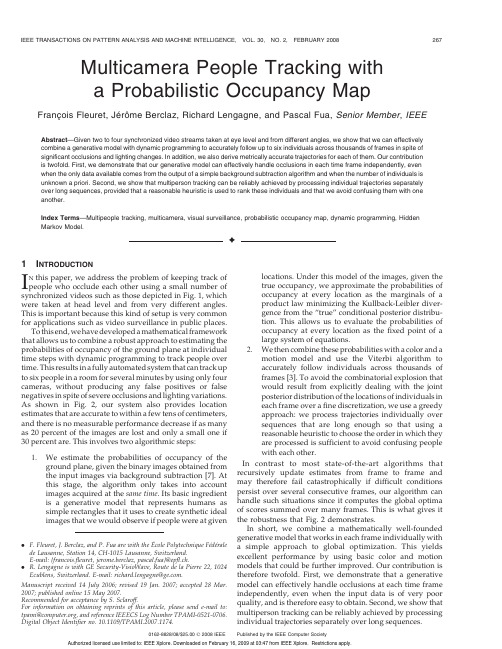
Multicamera People Tracking witha Probabilistic Occupancy MapFranc¸ois Fleuret,Je´roˆme Berclaz,Richard Lengagne,and Pascal Fua,Senior Member,IEEE Abstract—Given two to four synchronized video streams taken at eye level and from different angles,we show that we can effectively combine a generative model with dynamic programming to accurately follow up to six individuals across thousands of frames in spite of significant occlusions and lighting changes.In addition,we also derive metrically accurate trajectories for each of them.Our contribution is twofold.First,we demonstrate that our generative model can effectively handle occlusions in each time frame independently,even when the only data available comes from the output of a simple background subtraction algorithm and when the number of individuals is unknown a priori.Second,we show that multiperson tracking can be reliably achieved by processing individual trajectories separately over long sequences,provided that a reasonable heuristic is used to rank these individuals and that we avoid confusing them with one another.Index Terms—Multipeople tracking,multicamera,visual surveillance,probabilistic occupancy map,dynamic programming,Hidden Markov Model.Ç1I NTRODUCTIONI N this paper,we address the problem of keeping track of people who occlude each other using a small number of synchronized videos such as those depicted in Fig.1,which were taken at head level and from very different angles. This is important because this kind of setup is very common for applications such as video surveillance in public places.To this end,we have developed a mathematical framework that allows us to combine a robust approach to estimating the probabilities of occupancy of the ground plane at individual time steps with dynamic programming to track people over time.This results in a fully automated system that can track up to six people in a room for several minutes by using only four cameras,without producing any false positives or false negatives in spite of severe occlusions and lighting variations. As shown in Fig.2,our system also provides location estimates that are accurate to within a few tens of centimeters, and there is no measurable performance decrease if as many as20percent of the images are lost and only a small one if 30percent are.This involves two algorithmic steps:1.We estimate the probabilities of occupancy of theground plane,given the binary images obtained fromthe input images via background subtraction[7].Atthis stage,the algorithm only takes into accountimages acquired at the same time.Its basic ingredientis a generative model that represents humans assimple rectangles that it uses to create synthetic idealimages that we would observe if people were at givenlocations.Under this model of the images,given thetrue occupancy,we approximate the probabilities ofoccupancy at every location as the marginals of aproduct law minimizing the Kullback-Leibler diver-gence from the“true”conditional posterior distribu-tion.This allows us to evaluate the probabilities ofoccupancy at every location as the fixed point of alarge system of equations.2.We then combine these probabilities with a color and amotion model and use the Viterbi algorithm toaccurately follow individuals across thousands offrames[3].To avoid the combinatorial explosion thatwould result from explicitly dealing with the jointposterior distribution of the locations of individuals ineach frame over a fine discretization,we use a greedyapproach:we process trajectories individually oversequences that are long enough so that using areasonable heuristic to choose the order in which theyare processed is sufficient to avoid confusing peoplewith each other.In contrast to most state-of-the-art algorithms that recursively update estimates from frame to frame and may therefore fail catastrophically if difficult conditions persist over several consecutive frames,our algorithm can handle such situations since it computes the global optima of scores summed over many frames.This is what gives it the robustness that Fig.2demonstrates.In short,we combine a mathematically well-founded generative model that works in each frame individually with a simple approach to global optimization.This yields excellent performance by using basic color and motion models that could be further improved.Our contribution is therefore twofold.First,we demonstrate that a generative model can effectively handle occlusions at each time frame independently,even when the input data is of very poor quality,and is therefore easy to obtain.Second,we show that multiperson tracking can be reliably achieved by processing individual trajectories separately over long sequences.. F.Fleuret,J.Berclaz,and P.Fua are with the Ecole Polytechnique Fe´de´ralede Lausanne,Station14,CH-1015Lausanne,Switzerland.E-mail:{francois.fleuret,jerome.berclaz,pascal.fua}@epfl.ch..R.Lengagne is with GE Security-VisioWave,Route de la Pierre22,1024Ecublens,Switzerland.E-mail:richard.lengagne@.Manuscript received14July2006;revised19Jan.2007;accepted28Mar.2007;published online15May2007.Recommended for acceptance by S.Sclaroff.For information on obtaining reprints of this article,please send e-mail to:tpami@,and reference IEEECS Log Number TPAMI-0521-0706.Digital Object Identifier no.10.1109/TPAMI.2007.1174.0162-8828/08/$25.00ß2008IEEE Published by the IEEE Computer SocietyIn the remainder of the paper,we first briefly review related works.We then formulate our problem as estimat-ing the most probable state of a hidden Markov process and propose a model of the visible signal based on an estimate of an occupancy map in every time frame.Finally,we present our results on several long sequences.2R ELATED W ORKState-of-the-art methods can be divided into monocular and multiview approaches that we briefly review in this section.2.1Monocular ApproachesMonocular approaches rely on the input of a single camera to perform tracking.These methods provide a simple and easy-to-deploy setup but must compensate for the lack of 3D information in a single camera view.2.1.1Blob-Based MethodsMany algorithms rely on binary blobs extracted from single video[10],[5],[11].They combine shape analysis and tracking to locate people and maintain appearance models in order to track them,even in the presence of occlusions.The Bayesian Multiple-BLob tracker(BraMBLe)system[12],for example,is a multiblob tracker that generates a blob-likelihood based on a known background model and appearance models of the tracked people.It then uses a particle filter to implement the tracking for an unknown number of people.Approaches that track in a single view prior to computing correspondences across views extend this approach to multi camera setups.However,we view them as falling into the same category because they do not simultaneously exploit the information from multiple views.In[15],the limits of the field of view of each camera are computed in every other camera from motion information.When a person becomes visible in one camera,the system automatically searches for him in other views where he should be visible.In[4],a background/foreground segmentation is performed on calibrated images,followed by human shape extraction from foreground objects and feature point selection extraction. Feature points are tracked in a single view,and the system switches to another view when the current camera no longer has a good view of the person.2.1.2Color-Based MethodsTracking performance can be significantly increased by taking color into account.As shown in[6],the mean-shift pursuit technique based on a dissimilarity measure of color distributions can accurately track deformable objects in real time and in a monocular context.In[16],the images are segmented pixelwise into different classes,thus modeling people by continuously updated Gaussian mixtures.A standard tracking process is then performed using a Bayesian framework,which helps keep track of people,even when there are occlusions.In such a case,models of persons in front keep being updated, whereas the system stops updating occluded ones,which may cause trouble if their appearances have changed noticeably when they re-emerge.More recently,multiple humans have been simulta-neously detected and tracked in crowded scenes[20]by using Monte-Carlo-based methods to estimate their number and positions.In[23],multiple people are also detected and tracked in front of complex backgrounds by using mixture particle filters guided by people models learned by boosting.In[9],multicue3D object tracking is addressed by combining particle-filter-based Bayesian tracking and detection using learned spatiotemporal shapes.This ap-proach leads to impressive results but requires shape, texture,and image depth information as input.Finally, Smith et al.[25]propose a particle-filtering scheme that relies on Markov chain Monte Carlo(MCMC)optimization to handle entrances and departures.It also introduces a finer modeling of interactions between individuals as a product of pairwise potentials.2.2Multiview ApproachesDespite the effectiveness of such methods,the use of multiple cameras soon becomes necessary when one wishes to accurately detect and track multiple people and compute their precise3D locations in a complex environment. Occlusion handling is facilitated by using two sets of stereo color cameras[14].However,in most approaches that only take a set of2D views as input,occlusion is mainly handled by imposing temporal consistency in terms of a motion model,be it Kalman filtering or more general Markov models.As a result,these approaches may not always be able to recover if the process starts diverging.2.2.1Blob-Based MethodsIn[19],Kalman filtering is applied on3D points obtained by fusing in a least squares sense the image-to-world projections of points belonging to binary blobs.Similarly,in[1],a Kalman filter is used to simultaneously track in2D and3D,and objectFig.1.Images from two indoor and two outdoor multicamera video sequences that we use for our experiments.At each time step,we draw a box around people that we detect and assign to them an ID number that follows them throughout thesequence.Fig.2.Cumulative distributions of the position estimate error on a3,800-frame sequence(see Section6.4.1for details).locations are estimated through trajectory prediction during occlusion.In[8],a best hypothesis and a multiple-hypotheses approaches are compared to find people tracks from 3D locations obtained from foreground binary blobs ex-tracted from multiple calibrated views.In[21],a recursive Bayesian estimation approach is used to deal with occlusions while tracking multiple people in multiview.The algorithm tracks objects located in the intersections of2D visual angles,which are extracted from silhouettes obtained from different fixed views.When occlusion ambiguities occur,multiple occlusion hypotheses are generated,given predicted object states and previous hypotheses,and tested using a branch-and-merge strategy. The proposed framework is implemented using a customized particle filter to represent the distribution of object states.Recently,Morariu and Camps[17]proposed a method based on dimensionality reduction to learn a correspondence between the appearance of pedestrians across several views. This approach is able to cope with the severe occlusion in one view by exploiting the appearance of the same pedestrian on another view and the consistence across views.2.2.2Color-Based MethodsMittal and Davis[18]propose a system that segments,detects, and tracks multiple people in a scene by using a wide-baseline setup of up to16synchronized cameras.Intensity informa-tion is directly used to perform single-view pixel classifica-tion and match similarly labeled regions across views to derive3D people locations.Occlusion analysis is performed in two ways:First,during pixel classification,the computa-tion of prior probabilities takes occlusion into account. Second,evidence is gathered across cameras to compute a presence likelihood map on the ground plane that accounts for the visibility of each ground plane point in each view. Ground plane locations are then tracked over time by using a Kalman filter.In[13],individuals are tracked both in image planes and top view.The2D and3D positions of each individual are computed so as to maximize a joint probability defined as the product of a color-based appearance model and2D and 3D motion models derived from a Kalman filter.2.2.3Occupancy Map MethodsRecent techniques explicitly use a discretized occupancy map into which the objects detected in the camera images are back-projected.In[2],the authors rely on a standard detection of stereo disparities,which increase counters associated to square areas on the ground.A mixture of Gaussians is fitted to the resulting score map to estimate the likely location of individuals.This estimate is combined with a Kallman filter to model the motion.In[26],the occupancy map is computed with a standard visual hull procedure.One originality of the approach is to keep for each resulting connex component an upper and lower bound on the number of objects that it can contain. Based on motion consistency,the bounds on the various components are estimated at a certain time frame based on the bounds of the components at the previous time frame that spatially intersect with it.Although our own method shares many features with these techniques,it differs in two important respects that we will highlight:First,we combine the usual color and motion models with a sophisticated approach based on a generative model to estimating the probabilities of occu-pancy,which explicitly handles complex occlusion interac-tions between detected individuals,as will be discussed in Section5.Second,we rely on dynamic programming to ensure greater stability in challenging situations by simul-taneously handling multiple frames.3P ROBLEM F ORMULATIONOur goal is to track an a priori unknown number of people from a few synchronized video streams taken at head level. In this section,we formulate this problem as one of finding the most probable state of a hidden Markov process,given the set of images acquired at each time step,which we will refer to as a temporal frame.We then briefly outline the computation of the relevant probabilities by using the notations summarized in Tables1and2,which we also use in the following two sections to discuss in more details the actual computation of those probabilities.3.1Computing the Optimal TrajectoriesWe process the video sequences by batches of T¼100frames, each of which includes C images,and we compute the most likely trajectory for each individual.To achieve consistency over successive batches,we only keep the result on the first 10frames and slide our temporal window.This is illustrated in Fig.3.We discretize the visible part of the ground plane into a finite number G of regularly spaced2D locations and we introduce a virtual hidden location H that will be used to model entrances and departures from and into the visible area.For a given batch,let L t¼ðL1t;...;L NÃtÞbe the hidden stochastic processes standing for the locations of individuals, whether visible or not.The number NÃstands for the maximum allowable number of individuals in our world.It is large enough so that conditioning on the number of visible ones does not change the probability of a new individual entering the scene.The L n t variables therefore take values in f1;...;G;Hg.Given I t¼ðI1t;...;I C tÞ,the images acquired at time t for 1t T,our task is to find the values of L1;...;L T that maximizePðL1;...;L T j I1;...;I TÞ:ð1ÞAs will be discussed in Section 4.1,we compute this maximum a posteriori in a greedy way,processing one individual at a time,including the hidden ones who can move into the visible scene or not.For each one,the algorithm performs the computation,under the constraint that no individual can be at a visible location occupied by an individual already processed.In theory,this approach could lead to undesirable local minima,for example,by connecting the trajectories of two separate people.However,this does not happen often because our batches are sufficiently long.To further reduce the chances of this,we process individual trajectories in an order that depends on a reliability score so that the most reliable ones are computed first,thereby reducing the potential for confusion when processing the remaining ones. This order also ensures that if an individual remains in the hidden location,then all the other people present in the hidden location will also stay there and,therefore,do not need to be processed.FLEURET ET AL.:MULTICAMERA PEOPLE TRACKING WITH A PROBABILISTIC OCCUPANCY MAP269Our experimental results show that our method does not suffer from the usual weaknesses of greedy algorithms such as a tendency to get caught in bad local minima.We thereforebelieve that it compares very favorably to stochastic optimization techniques in general and more specifically particle filtering,which usually requires careful tuning of metaparameters.3.2Stochastic ModelingWe will show in Section 4.2that since we process individual trajectories,the whole approach only requires us to define avalid motion model P ðL n t þ1j L nt ¼k Þand a sound appearance model P ðI t j L n t ¼k Þ.The motion model P ðL n t þ1j L nt ¼k Þ,which will be intro-duced in Section 4.3,is a distribution into a disc of limited radiusandcenter k ,whichcorresponds toalooseboundonthe maximum speed of a walking human.Entrance into the scene and departure from it are naturally modeled,thanks to the270IEEE TRANSACTIONS ON PATTERN ANALYSIS AND MACHINE INTELLIGENCE,VOL.30,NO.2,FEBRUARY 2008TABLE 2Notations (RandomQuantities)Fig.3.Video sequences are processed by batch of 100frames.Only the first 10percent of the optimization result is kept and the rest is discarded.The temporal window is then slid forward and the optimiza-tion is repeated on the new window.TABLE 1Notations (DeterministicQuantities)hiddenlocation H,forwhichweextendthemotionmodel.The probabilities to enter and to leave are similar to the transition probabilities between different ground plane locations.In Section4.4,we will show that the appearance model PðI t j L n t¼kÞcan be decomposed into two terms.The first, described in Section4.5,is a very generic color-histogram-based model for each individual.The second,described in Section5,approximates the marginal conditional probabil-ities of occupancy of the ground plane,given the results of a background subtractionalgorithm,in allviewsacquired atthe same time.This approximation is obtained by minimizing the Kullback-Leibler divergence between a product law and the true posterior.We show that this is equivalent to computing the marginal probabilities of occupancy so that under the product law,the images obtained by putting rectangles of human sizes at occupied locations are likely to be similar to the images actually produced by the background subtraction.This represents a departure from more classical ap-proaches to estimating probabilities of occupancy that rely on computing a visual hull[26].Such approaches tend to be pessimistic and do not exploit trade-offs between the presence of people at different locations.For instance,if due to noise in one camera,a person is not seen in a particular view,then he would be discarded,even if he were seen in all others.By contrast,in our probabilistic framework,sufficient evidence might be present to detect him.Similarly,the presence of someone at a specific location creates an occlusion that hides the presence behind,which is not accounted for by the hull techniques but is by our approach.Since these marginal probabilities are computed indepen-dently at each time step,they say nothing about identity or correspondence with past frames.The appearance similarity is entirely conveyed by the color histograms,which has experimentally proved sufficient for our purposes.4C OMPUTATION OF THE T RAJECTORIESIn Section4.1,we break the global optimization of several people’s trajectories into the estimation of optimal individual trajectories.In Section 4.2,we show how this can be performed using the classical Viterbi’s algorithm based on dynamic programming.This requires a motion model given in Section 4.3and an appearance model described in Section4.4,which combines a color model given in Section4.5 and a sophisticated estimation of the ground plane occu-pancy detailed in Section5.We partition the visible area into a regular grid of G locations,as shown in Figs.5c and6,and from the camera calibration,we define for each camera c a family of rectangular shapes A c1;...;A c G,which correspond to crude human silhouettes of height175cm and width50cm located at every position on the grid.4.1Multiple TrajectoriesRecall that we denote by L n¼ðL n1;...;L n TÞthe trajectory of individual n.Given a batch of T temporal frames I¼ðI1;...;I TÞ,we want to maximize the posterior conditional probability:PðL1¼l1;...;L Nül NÃj IÞ¼PðL1¼l1j IÞY NÃn¼2P L n¼l n j I;L1¼l1;...;L nÀ1¼l nÀ1ÀÁ:ð2ÞSimultaneous optimization of all the L i s would beintractable.Instead,we optimize one trajectory after theother,which amounts to looking for^l1¼arg maxlPðL1¼l j IÞ;ð3Þ^l2¼arg maxlPðL2¼l j I;L1¼^l1Þ;ð4Þ...^l Nüarg maxlPðL Nül j I;L1¼^l1;L2¼^l2;...Þ:ð5ÞNote that under our model,conditioning one trajectory,given other ones,simply means that it will go through noalready occupied location.In other words,PðL n¼l j I;L1¼^l1;...;L nÀ1¼^l nÀ1Þ¼PðL n¼l j I;8k<n;8t;L n t¼^l k tÞ;ð6Þwhich is PðL n¼l j IÞwith a reduced set of the admissiblegrid locations.Such a procedure is recursively correct:If all trajectoriesestimated up to step n are correct,then the conditioning onlyimproves the estimate of the optimal remaining trajectories.This would suffice if the image data were informative enoughso that locations could be unambiguously associated toindividuals.In practice,this is obviously rarely the case.Therefore,this greedy approach to optimization has un-desired side effects.For example,due to partly missinglocalization information for a given trajectory,the algorithmmight mistakenly start following another person’s trajectory.This is especially likely to happen if the tracked individualsare located close to each other.To avoid this kind of failure,we process the images bybatches of T¼100and first extend the trajectories that havebeen found with high confidence,as defined below,in theprevious batches.We then process the lower confidenceones.As a result,a trajectory that was problematic in thepast and is likely to be problematic in the current batch willbe optimized last and,thus,prevented from“stealing”somebody else’s location.Furthermore,this approachincreases the spatial constraints on such a trajectory whenwe finally get around to estimating it.We use as a confidence score the concordance of theestimated trajectories in the previous batches and thelocalization cue provided by the estimation of the probabil-istic occupancy map(POM)described in Section5.Moreprecisely,the score is the number of time frames where theestimated trajectory passes through a local maximum of theestimated probability of occupancy.When the POM does notdetect a person on a few frames,the score will naturallydecrease,indicating a deterioration of the localizationinformation.Since there is a high degree of overlappingbetween successive batches,the challenging segment of atrajectory,which is due to the failure of the backgroundsubtraction or change in illumination,for instance,is met inseveral batches before it actually happens during the10keptframes.Thus,the heuristic would have ranked the corre-sponding individual in the last ones to be processed whensuch problem occurs.FLEURET ET AL.:MULTICAMERA PEOPLE TRACKING WITH A PROBABILISTIC OCCUPANCY MAP2714.2Single TrajectoryLet us now consider only the trajectory L n ¼ðL n 1;...;L nT Þof individual n over T temporal frames.We are looking for thevalues ðl n 1;...;l nT Þin the subset of free locations of f 1;...;G;Hg .The initial location l n 1is either a known visible location if the individual is visible in the first frame of the batch or H if he is not.We therefore seek to maximizeP ðL n 1¼l n 1;...;L n T ¼l nt j I 1;...;I T Þ¼P ðI 1;L n 1¼l n 1;...;I T ;L n T ¼l nT ÞP ðI 1;...;I T Þ:ð7ÞSince the denominator is constant with respect to l n ,we simply maximize the numerator,that is,the probability of both the trajectories and the images.Let us introduce the maximum of the probability of both the observations and the trajectory ending up at location k at time t :Èt ðk Þ¼max l n 1;...;l nt À1P ðI 1;L n 1¼l n 1;...;I t ;L nt ¼k Þ:ð8ÞWe model jointly the processes L n t and I t with a hidden Markov model,that isP ðL n t þ1j L n t ;L n t À1;...Þ¼P ðL n t þ1j L nt Þð9ÞandP ðI t ;I t À1;...j L n t ;L nt À1;...Þ¼YtP ðI t j L n t Þ:ð10ÞUnder such a model,we have the classical recursive expressionÈt ðk Þ¼P ðI t j L n t ¼k Þ|fflfflfflfflfflfflfflfflffl{zfflfflfflfflfflfflfflfflffl}Appearance modelmax P ðL n t ¼k j L nt À1¼ Þ|fflfflfflfflfflfflfflfflfflfflfflfflfflfflfflfflffl{zfflfflfflfflfflfflfflfflfflfflfflfflfflfflfflfflffl}Motion modelÈt À1ð Þð11Þto perform a global search with dynamic programming,which yields the classic Viterbi algorithm.This is straight-forward,since the L n t s are in a finite set of cardinality G þ1.4.3Motion ModelWe chose a very simple and unconstrained motion model:P ðL n t ¼k j L nt À1¼ Þ¼1=Z Áe À k k À k if k k À k c 0otherwise ;&ð12Þwhere the constant tunes the average human walkingspeed,and c limits the maximum allowable speed.This probability is isotropic,decreases with the distance from location k ,and is zero for k k À k greater than a constantmaximum distance.We use a very loose maximum distance cof one square of the grid per frame,which corresponds to a speed of almost 12mph.We also define explicitly the probabilities of transitions to the parts of the scene that are connected to the hidden location H .This is a single door in the indoor sequences and all the contours of the visible area in the outdoor sequences in Fig.1.Thus,entrance and departure of individuals are taken care of naturally by the estimation of the maximum a posteriori trajectories.If there are enough evidence from the images that somebody enters or leaves the room,then this procedure will estimate that the optimal trajectory does so,and a person will be added to or removed from the visible area.4.4Appearance ModelFrom the input images I t ,we use background subtraction to produce binary masks B t such as those in Fig.4.We denote as T t the colors of the pixels inside the blobs and treat the rest of the images as background,which is ignored.Let X tk be a Boolean random variable standing for the presence of an individual at location k of the grid at time t .In Appendix B,we show thatP ðI t j L n t ¼k Þzfflfflfflfflfflfflfflfflffl}|fflfflfflfflfflfflfflfflffl{Appearance model/P ðL n t ¼k j X kt ¼1;T t Þ|fflfflfflfflfflfflfflfflfflfflfflfflfflfflfflfflfflffl{zfflfflfflfflfflfflfflfflfflfflfflfflfflfflfflfflfflffl}Color modelP ðX kt ¼1j B t Þ|fflfflfflfflfflfflfflfflfflfflffl{zfflfflfflfflfflfflfflfflfflfflffl}Ground plane occupancy:ð13ÞThe ground plane occupancy term will be discussed in Section 5,and the color model term is computed as follows.4.5Color ModelWe assume that if someone is present at a certain location k ,then his presence influences the color of the pixels located at the intersection of the moving blobs and the rectangle A c k corresponding to the location k .We model that dependency as if the pixels were independent and identically distributed and followed a density in the red,green,and blue (RGB)space associated to the individual.This is far simpler than the color models used in either [18]or [13],which split the body area in several subparts with dedicated color distributions,but has proved sufficient in practice.If an individual n was present in the frames preceding the current batch,then we have an estimation for any camera c of his color distribution c n ,since we have previously collected the pixels in all frames at the locations272IEEE TRANSACTIONS ON PATTERN ANALYSIS AND MACHINE INTELLIGENCE,VOL.30,NO.2,FEBRUARY2008Fig.4.The color model relies on a stochastic modeling of the color of the pixels T c t ðk Þsampled in the intersection of the binary image B c t produced bythe background subtraction and the rectangle A ck corresponding to the location k .。
无人驾驶的英语课件PPT

Other potential applications include long haul trucking, public transportation, and even self driving taxis or shared mobility services
3D Reconstruction
The creation of a 3D model of the environment from sensor data to provide more accurate representation of the scene
Path planning technology
Application scenarios for autonomous driving
Autonomous driving has the potential to revolutionize transportation, particularly in urban areas where traffic congestion and pollution are major issues
Techniques used to regulate the vehicle's velocity, acceleration, and steel angle to achieve desired performance and safety standards
Risk Assessment
The evaluation of potential hazards and their associated risks to inform decision making processes
longitudinal 名词

longitudinal 名词longitudinal的英语名词是"longitudinal",意思是指与纵向或经度有关的事物或特征。
1. The study examined the longitudinal effects of smoking on lung health.该研究考察了吸烟对肺健康的纵向影响。
2. Longitudinals are the vertical beams that support the roof of the building.纵梁是支撑建筑物屋顶的垂直梁。
3. The longitudinal lines on a globe represent the meridians of longitude.地球仪上的纵线代表经线。
4. A longitudinal study was conducted to track the development of cognitive abilities in children over a period of 10 years.进行了一项长期研究,追踪儿童10年来的认知能力发展。
5. The researcher used longitudinal data to analyze the trends in employment rates over the past decade.研究人员使用纵向数据分析了过去十年就业率的趋势。
6. The longitudinal study revealed that regular exercise has long-term health benefits.纵向研究揭示了经常锻炼对长期健康的益处。
7. The longitudinal waves in the ocean are responsible for the motion of surfers.海洋中的纵波控制着冲浪者的运动。
小学上册第十二次英语第六单元测验试卷

小学上册英语第六单元测验试卷英语试题一、综合题(本题有100小题,每小题1分,共100分.每小题不选、错误,均不给分)1.I like to watch _____ fly near the flowers.2. A gardener must know how to care for different ______. (园丁必须知道如何照顾不同的植物。
)3.We can see many ________ (野生动物) in the national park.4.My _______ (狗) follows me everywhere.5.My dad drives a _____ (car/bike).6.The Earth's tilt causes the ______.7.I like to go ______ (散步) in the evening.8. A fault is a crack in the Earth’s crust where movement has occurred, often causing ______.9.The chemical symbol for iodine is __________.10.How do you say "bird" in Spanish?A. PájaroB. OiseauC. VogelD. Uccello11.My brother loves to read ____.12.What do we call a group of butterflies?A. FlutterB. SwarmC. KaleidoscopeD. FlightC Kaleidoscope13. A homogeneous mixture has a _____ composition throughout.14.What is the color of a ripe strawberry?A. BlueB. GreenC. RedD. Yellow15.The cake is ________ (松软).16.What do we use to write on paper?A. PaintB. PencilC. BrushD. Marker17.The stars are _____ (twinkling/shining) in the sky.18.I brush my teeth _____ morning. (every)19.The elephant is the largest _______ (大象是最大的_______).20. A ______ (果实) grows from the flower after fertilization.21.My favorite color is ___. (blue, book, tree)22.What is the capital of Kazakhstan?A. AlmatyB. AstanaC. BishkekD. TashkentB23.I have a toy _____ that bounces.24.Which ocean is the largest?A. Atlantic OceanB. Indian OceanC. Arctic OceanD. Pacific OceanD25.She is wearing a ______ dress. (red)26.What do we call a baby dog?A. KittenB. PuppyC. CubD. Calf27. A _______ can help to visualize the relationship between force and motion.28.Which of these is a type of fruit?A. PotatoB. BeanC. PeachD. LettuceC29.What is the primary language spoken in the USA?A. SpanishB. FrenchC. EnglishD. ChineseC30.The freezing point of water is _____ degrees Celsius.31.What is the opposite of 'happy'?A. SadB. JoyfulC. ExcitedD. Angry32.The puppy sleeps in a _______ (小狗在_______里睡觉).33.What is the color of a school bus?A. BlueB. GreenC. YellowD. Red34.They are ___ a game. (playing)35.Plants need ______ (二氧化碳) to perform photosynthesis.36. A __________ is a reaction that produces energy in the form of light.37.What is the main ingredient in French fries?A. PotatoB. CornC. RiceD. WheatA38.desert) is a dry area with little rainfall. The ____39.What do you call the study of the stars and planets?A. BiologyB. ChemistryC. AstronomyD. GeographyC40.The ancient Chinese invented _______ during the Han dynasty. (火药)41.What is the sum of 5 + 6?A. 10B. 11C. 12D. 13B42.The gecko climbs walls with its _________. (脚)43.The ____ has a slender body and is often found in the grass.44.I want to create a ________ in my backyard.45.What do you call a person who takes care of animals?A. VeterinarianB. ZookeeperC. FarmerD. GardenerA46.In a ______ change, the substance's identity does not change.47. A snail leaves a ______ (黏糊糊的) trail behind.48.What is the name of the famous wizard in J.K. Rowling's series?A. Frodo BagginsB. Harry PotterC. GandalfD. Albus DumbledoreB49.What do you call the place where you go to learn?A. StoreB. SchoolC. FactoryD. Office50.Plants can be studied for ______ (科学研究).51.Which animal is known as man's best friend?A. CatB. DogC. HorseD. FishB52.Which season comes after winter?A. FallB. SummerC. SpringD. Rainy53.What is the primary color of grass?A. RedB. YellowC. BlueD. GreenD54.The cake is ___ (frosted).55.The sun is ________ (温暖) in spring.56.The _______ (小蜻蜓) catches insects in the air.57.The Earth's surface is influenced by both human and ______ activities.58. A reaction that occurs in an aqueous solution is called a ______ reaction.59.The room is _______ (明亮的).60.The rabbit loves to hop around the _________. (院子)61.What animal is known for having stripes?A. LionB. TigerC. BearD. ElephantB62.The garden is ________ (生机勃勃).63.My teacher is _______ and makes learning fun.64.The ______ (水果) of a plant is often sweet and nutritious.65._____ (sustainable) practices help the environment.66. A comet has a bright ______ that can be seen from Earth.67. A __________ is a small island. (小岛)68.My favorite season is ______ (秋天).69.The _______ grows best in moist environments.70.My favorite flower is a ______.71.What do we call the imaginary line that divides the Earth into the Eastern and Western hemispheres?A. EquatorB. Prime MeridianC. LatitudeD. LongitudeB72.I like to sing ______ songs with my friends.73.Ancient Chinese invented ________ to keep track of time.74.I love to learn about plants and how they ________ (生长) in different environments.75.Learning about plants can inspire ______ (环保) efforts.76.What is the primary function of roots in plants?A. Absorb sunlightB. Absorb water and nutrientsC. Produce flowersD. Support the plantB77.The sun is shining ________.78.The chemical formula for silver bromide is _____.79. A chemical reaction that occurs when two substances combine is called a ______ reaction.80.What do you call a baby cat?A. PuppyB. KittenC. CubD. FawnB81. A lion's pride consists of related females and a few ________________ (雄性).82.What is the term for the study of insects?A. EntomologyB. OrnithologyC. ZoologyD. BotanyA83.What do bees make?A. MilkB. HoneyC. BreadD. CheeseB84.Objects in motion tend to stay in ______.85.I brush my teeth _____ (every/never) day.86.The ______ (木本植物) includes trees and shrubs.87.Planting in layers can create a ______ (多层次) garden.88.My grandmother loves to knit __________ (围巾).89.What do we call a group of stars?A. GalaxyB. ClusterC. ConstellationD. NebulaC90.The __________ is a region known for its festivals.91.What do we call the study of the Earth?A. BiologyB. GeographyC. ChemistryD. PhysicsB92.I see _____ birds flying. (many)93.The _______ of light can create various effects in photography.94.She likes to _______ (play) the piano.95.Planting trees can help combat _____ (全球变暖).96.I like _____ (sharing) my gardening tips with others.97.My dad loves to watch _____ (比赛) on TV.98.What is the main language spoken in Spain?A. FrenchB. SpanishC. ItalianD. PortugueseB Spanish99.The ______ (海龟) swims gracefully in the ocean.100.I found a ______ in my pocket. (button)。
2021年北京市丰台区高三一模英语试题[附答案]
![2021年北京市丰台区高三一模英语试题[附答案]](https://img.taocdn.com/s3/m/648b051b0c22590103029d61.png)
丰台区2021年高三年级第二学期综合练习(一)英语2021.03本试卷满分共100分考试时间90分钟注意事项:1.答题前,考生务必先将答题卡上的学校、年级、班级、姓名、准考证号用黑色字迹签字笔填写清楚,并认真核对条形码上的准考证号、姓名,在答题卡的“条形码粘贴区”贴好条形码。
2.本次考试所有答题均在答题卡上完成。
选择题必须使用2B铅笔以正确填涂方式将各小题对应选项涂黑,如需改动,用橡皮擦除干净后再选涂其它选项。
非选择题必须使用标准黑色字迹签字笔书写,要求字体工整、字迹清楚3.请严格按照答题卡上题号在相应答题区内作答,超出答题区域书写的答案无效,在试卷、草稿纸上答题无效。
4.请保持答题卡卡面清洁,不要装订、不要折叠、不要破损。
第一部分:知识运用(共两节,30分)第一节完形填空(共10小题;每小题1.5分,共15分)阅读下面短文,掌握其大意,从每题所给的A、B、C、D四个选项中,选出最佳选项,并在答题卡上将该项涂黑。
This was the fifth time I’d been to the National Annual Competition. Reporters had been saying that I looked unbeatable. Everyone expected me to __1__. But I knew something was __2__ because I couldn’t get this one picture out of my head; a picture of me, falling. “Go away,” I’d say, But the image wouldn’t __3__.It was time to skate. The music started, slowly, and I told myself, “Have fun, Michael! It’s just a(n) __4__.”Once the music picked up, I started skating faster, I’d practiced the routine so manytimes, and I didn’t have to think about __5__ came next. But when I came down from thejump, my foot slipped from under me. I put a hand on the ice to __6__ myself, but it didn’tdo any good.Things kept getting __7__. On a triple flip(三周跳) I spun through the air, and justas I landed, my whole body went down again. There I was, flat on the ice, with the whole world __8__.I didn’t think I’d be able to pull myself together. But as I got up, I heard an amazing __9__. People were clapping in time to the music. They were trying to give me courage.I wasn’t surprised by my scores. However, the audience’s clapping woke me up! I was so busy trying not to __10__ that I forgot to feel what was in my heart—the love for skating.1. A. win B. enjoy C. share D. relax2. A. challenging B. missing C. wrong D. dangerous3. A. return B. leave C. appear D. stay4. A. sport B. activity C. picture D. accident5. A. when B. why C. who D. what6. A. prepare B. catch C. comfort D. measure7. A. clearer B. easier C. heavier D. worse8. A. watching B. expecting C. ignoring D. changing9. A. voice B. story C. sound D. idea10. A. collapse B. resist C. fall D. escape第二节语法填空(共10小题;每小题1.5分,共15分)阅读下列短文,根据短文内容填空,在未给提示词的空白处仅填写1个适当的单词,在给出提示词的空白处用括号内所给词的正确形式填空。
Eighth+grade+first+volume+English+full+volume+cour

Teach students how to manage their time effectively and complete tasks within a reasonable time frame
要点三
ห้องสมุดไป่ตู้
Textbooks and workbooks
Provide students with textbooks and workbooks that are well organized, easy to understand, and contain a variety of exercises and activities to help them practice and review
Memory skills
Introduce effective vocabulary memory methods, such as root and affix methods, associative memory methods, etc., to help students quickly memorize words and improve learning efficiency.
To develop students' ability to think critically and analytically about the information they received in English, enabling them to make informed decisions and judgments
小学上册第九次英语第1单元暑期作业

小学上册英语第1单元暑期作业英语试题一、综合题(本题有100小题,每小题1分,共100分.每小题不选、错误,均不给分)1.The _______ can bring colors to your life.2.The _____ (火焰) is warm.3.What do we call a large body of saltwater?A. RiverB. LakeC. OceanD. PondC4.What do we call the process of removing trees from a forest?A. ReforestationB. AfforestationC. DeforestationD. ConservationC Deforestation5.My best friend is very ______.6.What is the name of the famous American author known for his short stories?A. Edgar Allan PoeB. Nathaniel HawthorneC. F. Scott FitzgeraldD. All of the aboveD7.The chemical formula for acetic acid is _______.8. A solution is a homogeneous mixture of two or more _____.9.The sun is _____ in the sky. (high)10.The _______ is a measure of how much solute is in a solution.11. A force can cause an object to ______.12.My ______ is a great storyteller.13.Potential energy is stored ______.14.What do we call a young dolphin?A. CalfB. PupC. KidD. Foal15.What is the main gas in the atmosphere?A. OxygenB. NitrogenC. Carbon DioxideD. HydrogenB16.What is the term for animals that live both on land and in water?A. MammalsB. ReptilesC. AmphibiansD. Fish17.What do we use to write on paper?A. BrushB. PencilC. SpoonD. Scissors18.My sister loves to _____ her dolls. (play with)19.What do we call a young hedgehog?A. HogletB. PupC. KitD. CalfA Hoglet20.The ________ (strategy) guides our efforts.21.What is the largest planet in our solar system?A. EarthB. MarsC. JupiterD. Saturn22.The _____ (rainbow) appears after a storm.23.My favorite fruit is ___ (apple/banana).24. A __________ (植物的繁殖) can be done in various ways.25.What do you call a young eagle?A. ChickB. EyassC. EagletD. CalfC26.I enjoy learning about health and ______ (营养). It’s important to take care of our bodies.27.My favorite subject is _____ (math/science).28.She has a big _____ (狗).29.The __________ (历史的平衡) requires multiple viewpoints.30.What is the name of the famous mountain in the United States?A. Mount EverestB. Mount RushmoreC. Mount KilimanjaroD. Mount Fuji31.What do you call the tool used for cutting paper?A. KnifeB. ScissorsC. StaplerD. Ruler32.What is the name of the fairy tale character who had a red cape?A. CinderellaB. Little Red Riding HoodC. Snow WhiteD. Belle33. A dolphin is a playful _______ that loves to swim and jump through the waves.34. A ______ is a method for analyzing scientific data.35.The girl sings very ________.36.My favorite fruit is __________ because it tastes __________.37.The ______ of a cactus helps it survive in dry conditions. (仙人掌的刺帮助它在干燥的环境中生存。
计算机视觉在人体运动分析中的应用

计算机视觉在人体运动分析中的应用一、介绍计算机视觉是计算机科学中的一个重要领域,它研究如何让计算机“看得”懂图像和视频。
人体运动分析是计算机视觉的一个应用领域,旨在分析一个人的运动方式和姿势。
人体运动分析在医学、体育、娱乐等领域都有广泛的应用。
二、传统方法和新技术传统的人体运动分析方法主要依靠专业的人工观察和判断。
例如,在体育比赛中,裁判员需要根据运动员的姿态和位置判断是否犯规。
但是,这种方法存在一些问题,例如判断结果可能不够准确、耗时长、需要专业人员和设备等等。
随着计算机视觉技术的发展,许多新的方法和技术被应用到人体运动分析中,例如机器学习、深度学习、三维重建等。
这些新技术不仅提高了准确性,而且大大降低了成本和人工工作量。
三、人体姿态估计人体姿态估计是指根据图像或视频中人的姿势来进行姿态分析。
近几年,深度神经网络(DNN)被广泛应用于人体姿态估计中。
DNN可以学习人体姿态和关节点的特征,从而准确地估计人体姿态。
此外,3D骨架提取技术也被应用于人体姿态估计中。
通过分析视频序列中的每帧图像,该技术可以估计人体的三维姿态。
四、运动跟踪人体运动跟踪通常是指在视频序列中跟踪和分析一个或多个运动对象的位置、速度和加速度等。
传统方法使用人工跟踪或者基于运动模型的方法。
许多新技术已经应用于运动跟踪中。
例如,深度学习可以通过学习图像序列中对象的运动特征,跟踪对象的位置和速度。
此外,利用时空立方体来描述动作划分和物体跟踪也被广泛应用于运动跟踪。
五、动作识别和分类动作识别和分类通常用于将视频序列中的行为/动作或运动样式分类。
这个研究领域可以帮助人们理解运动样式、分类体育项目或研究人类行为模式。
深度学习几乎已经成为动作识别和分类的标准技术。
通过学习时空特征和动作之间的关系,深度学习可以在很大程度上提高动作分类的准确性和可靠性。
六、应用案例计算机视觉在人体运动分析中的应用已经有许多成功的案例。
在体育领域,计算机视觉可以帮助评估运动员的运动表现和强化训练。
- 1、下载文档前请自行甄别文档内容的完整性,平台不提供额外的编辑、内容补充、找答案等附加服务。
- 2、"仅部分预览"的文档,不可在线预览部分如存在完整性等问题,可反馈申请退款(可完整预览的文档不适用该条件!)。
- 3、如文档侵犯您的权益,请联系客服反馈,我们会尽快为您处理(人工客服工作时间:9:00-18:30)。
Learning to Track3D Human Motion from SilhouettesAnkur Agarwal ANKUR.AGARWAL@INRIALPES.FR Bill Triggs BILL.TRIGGS@INRIALPES.FR GRA VIR-INRIA-CNRS,655Avenue de l’Europe,Montbonnot38330,FranceAbstractWe describe a sparse Bayesian regression methodfor recovering3D human body motion directlyfrom silhouettes extracted from monocular videosequences.No detailed body shape model isneeded,and realism is ensured by training on realhuman motion capture data.The tracker esti-mates3D body pose by using Relevance VectorMachine regression to combine a learned autore-gressive dynamical model with robust shape de-scriptors extracted automatically from image sil-houettes.We studied several different combina-tion methods,the most effective being to learna nonlinear observation-update correction basedon joint regression with respect to the predictedstate and the observations.We demonstrate themethod on a54-parameter full body pose model,both quantitatively using motion capture basedtest sequences,and qualitatively on a test videosequence.1.IntroductionWe consider the problem of estimating and tracking the3D configurations of complex articulated objects from monoc-ular images,e.g.for applications requiring3D human body pose or hand gesture analysis.There are two main schools of thought on this.Model-based approaches presuppose an explicitly known parametric body model,and estimate the pose by either:(i)directly inverting the kinemat-ics,which requires known image positions for each body part(Taylor,2000);or(ii)numerically optimizing some form of model-image correspondence metric over the pose variables,using a forward rendering model to predict the images,which is expensive and requires a good initial-ization,and the problem always has many local minima (Sminchisescu&Triggs,2003).An important sub-case is model-based tracking,which focuses on tracking the pose Appearing in Proceedings of the21st International Conference on Machine Learning,Banff,Canada,2004.Copyright2004by the authors.estimate from one time step to the next starting from a known initialization,based on an approximate dynamical model(Bregler&Malik,1998,Sidenbladh et al.,2002).In contrast,learning based approaches try to avoid the need for accurate3D modelling and rendering,and to capitalize on the fact that the set of typical human poses is far smaller than the set of kinematically possible ones,by estimating (learning)a model that directly recovers pose estimates from observable image quantities(Grauman et al.,2003). In particular,example based methods explicitly store a set of training examples whose3D poses are known, and estimate pose by searching for training image(s)sim-ilar to the given input image,and interpolating from their poses(Athitsos&Sclaroff,2003,Stenger et al.,2003, Mori&Malik,2002,Shakhnarovich et al.,2003).In this paper we take a learning based approach,but in-stead of explicitly storing and searching for similar training examples,we use sparse Bayesian nonlinear regression to distill a large training database into a single compact model that generalizes well to unseen examples.We regress the current pose(body joint angles)against both image descrip-tors(silhouette shape)and a pose estimate computed from previous poses using a learned dynamical model.High di-mensionality and the intrinsic ambiguity in recovering pose from monocular observations makes the regression nontriv-ial.Our algorithm can be related to probabilistic tracking, but we eliminate the need for:(i)an exact body model that must be projected to predict an image;and(ii)a pre-defined error model to evaluate the likelihood of the ob-served image signal given this projection.Instead,pose is estimated directly,by regressing it against a dynamics-based prediction and an observed shape descriptor vector. Regressing on shape descriptors allows appearance varia-tions to be learned automatically,enabling us to work with a simple generic articular skeleton model;while including an estimate of the pose in the regression allows the method to overcome the inherent many-to-one projection ambigui-ties present in monocular image observations.Our strategy makes good use of the sparsity and generaliza-tion properties of our nonlinear regressor,which is a variant of the Relevance Vector Machine(RVM)(Tipping,2000).RVM’s have been used,e.g.,to build kernel regressors for 2D displacement updates in correlation-based patch track-ing (Williams et al.,2003).Human pose recovery is sig-nificantly harder —more ill-conditioned and nonlinear,and much higher dimensional —but by selecting a suffi-ciently rich set of image descriptors,it turns out that we can still obtain enough information for successful regres-sion (Agarwal &Triggs,2004a).Our motion capture based training data models each joint as a spherical one,so formally,we represent 3D body pose by 55-D vectors x including 3joint angles for each of the 18major body joints.The input images are reduced to 100-D observation vectors z that robustly encode the shape of a human image silhouette.Given a temporal sequence of observations z t ,the goal is to estimate the correspond-ing sequence of pose vectors x t .We work as follows:At each time step,we obtain an approximate preliminarypose estimate ˇxt from the previous two pose vectors,us-ing a dynamical model learned by linear least squares re-gression.We then update this to take account of the ob-servations z t using a joint RVM regression over ˇxt and z t —x =r (ˇx ,z )—learned from a set of labelled training examples {(z i ,x i )|i =1...n }.The regressor is a lin-ear combination r (x ,z )≡ k a k φk (x ,z )of prespecified scalar basis functions {φk (x ,z )|k =1...p }(here,instan-tiated Gaussian kernels).The learned regressor is regular in the sense that the weight vectors a k are well-damped to control over-fitting,and sparse in the sense that many of them are zero.Sparsity occurs because the RVM actively selects only the ‘most relevant’basis functions —the ones that really need to have nonzero coefficients to complete the regression successfully.Previous work:There is a good deal of prior work on hu-man pose analysis,but relatively little on directly learning 3D pose from image measurements.(Brand,1999)models a dynamical manifold of human body configurations with a Hidden Markov Model and learns using entropy minimiza-tion.(Athitsos &Sclaroff,2000)learn a perceptron map-ping between the appearance and parameter spaces.Human pose is hard to ground truth,so most papers in this area use only heuristic visual inspection to judge their results.How-ever,the interpolated-k -nearest-neighbor learning method of (Shakhnarovich et al.,2003)used a human model ren-dering package (P OSER from Curious Labs)to synthesize ground-truthed training and test images of 13degree of freedom upper body poses with a limited (±40◦)set of ran-dom torso movements and view points,obtaining RMS es-timation errors of about 20◦per d.o.f.In comparison,our regression algorithm estimates full 54d.o.f.body pose and orientation —a problem whose high dimensionality would really stretch the capacity of an example based method such as (Shakhnarovich et al.,2003)—with mean errors of only about 4◦.We also used P OSER to synthesize a largesetFigure 1.Different 3D poses can have very similar image obser-vations,causing the regression from image silhouettes to 3D pose to be inherently multi-valued.of training and test images from different viewpoints,but rather than using random synthetic poses,we used poses taken from real human motion capture sequences.Our re-sults thus relate to real poses and we also capture the dy-namics of typical human motions for temporal consistency.The motion capture data was taken from the public website /graphics/animWeb/humanoid .(Howe et al.,1999)developed a Bayesian learning frame-work to recover 3D pose from known image locations of body joint centres,based on a training set of pose-centre pairs obtained from resynthesized motion capture data.(Mori &Malik,2002)estimate the centres using shape con-text image matching against a set of training images with pre-labelled centres,then reconstruct 3D pose using the al-gorithm of (Taylor,2000).Rather than working indirectly via joint centres,we chose to estimate pose directly from the underlying image descriptors,as we feel that this is likely to prove both more accurate and more robust,pro-viding a generic framework for estimating and tracking any prespecified set of parameters from image observations.(Pavlovic et al.,2000,Ormoneit et al.,2000)learn dynami-cal models for specific human motions.Particle filters and MCMC methods have widely been used in probabilistic tracking frameworks e.g .(Sidenbladh et al.,2002).Most of the previous learning based methods for human track-ing take a generative,model based approach,whereas our approach is essentially discriminative.2.Observations as Shape DescriptorsTo improve resistance to segmentation errors and occlu-sions,we use a robust representation for our image ob-servations.Of the many different image descriptors that could be used for human pose estimation,and in line with (Brand,1999,Athitsos &Sclaroff,2000),we have chosen to base our system on image silhouettes.There are twomain problems with silhouettes:(i)Artifacts such as shadow attachment and poor background segmentation tend to distort their local form.This often causes problems when global descriptors such as shape moments are used,as in (Brand,1999,Athitsos&Sclaroff,2000),because each lo-cal error pollutes every component of the descriptor.To be robust,shape descriptors must have good spatial local-ity.(ii)Silhouettes make several discrete and continuous degrees of freedom invisible or poorly visible.It is diffi-cult to tell frontal views from back ones,whether a person seen from the side is stepping with the left leg or the right one,and what are the exact poses of arms or hands that fall within(are‘occluded’by)the torso’s silhouette(see fig.1).These factors limit the performance attainable from silhouette-based methods.Histograms of edge information are a good way to encode local shape robustly(Lowe,1999).Here,we use shape con-texts(histograms of local edge pixels into log-polar bins) (Belongie et al.,2002)to encode silhouette shape quasi-locally over a range of scales,making use of their locality properties and capability to encode approximate spatial po-sition on the silhouette—see(Agarwal&Triggs,2004a). Unlike Belognie et al,we use quite small image regions (roughly the size of a limb)to compute our shape contexts, and for increased locality,we normalize each shape con-text histogram only by the number of points in its region. This is essential for robustness against occlusions,shad-ows,etc.The shape context distributions of all edge points on a silhouette are reduced to100-D histograms by vec-tor quantizing the60-D shape context space using Gaussian weights to vote softly into the few histogram centres nearest to the contexts.This softening allows us to compare his-tograms using simple Euclidean distance rather than,say, Earth Movers Distance(Rubner et al.,1998).Each image observation(silhouette)is thusfinally reduced to a100-D quantized-distribution-of-shape-context vector,giving rea-sonably good robustness to occlusions and to local silhou-ette segmentation failures.3.Tracking and RegressionThe3D pose can only be observed indirectly via ambiguous and noisy image measurements,so it is appropriate to start by considering the Bayesian tracking framework in which our knowledge about the state(pose)x t given the observa-tions up to time t is represented by a probability distribu-tion,the posterior state density p(x t|z t,z t−1,...,z0). Given an image observation z t and a prior p(x t)on the corresponding pose x t,the posterior likelihood for x t is usually evaluated using Bayes’rule,p(x t|z t)∝p(z t|x t)p(x t),where p(z t|x t)is a precise‘generative’ob-servation model that predicts z t and its uncertainty given x t.Unfortunately,when tracking objects as complicated as the human body,the observations depend on a great many factors that are difficult to control,ranging from lighting and background to body shape and clothing style and tex-ture,so any hand-built observation model is necessarily a gross oversimplification.One way around this would be to learn the generative model p(z|x)from examples,then to work backwards via its Ja-cobian to get a linearized state update,as in the extended Kalmanfilter.However,this approach is somewhat indirect, and it may waste a considerable amount of effort modelling appearance details that are irrelevant for predicting pose. Instead,we prefer to learn a‘discriminative’(diagnostic or anti-causal)model p(x|z)for the pose x given the obser-vations z—c.f.the difference between generative and dis-criminative classification,and the regression based trackers of(Jurie&Dhome,2002,Williams et al.,2003).Similarly, in the context of maximum likelihood pose estimation,we would prefer to learn a‘diagnostic’regressor x=x(z), i.e.a point estimator for the most likely state x given the observations z,not a generative predictor z=z(x). Unfortunately,this brings up a second problem.In monocu-lar human pose reconstruction,image projection suppresses most of the depth(camera-object distance)information,so the state-to-observation mapping is always many-to-one.In fact,even when the labelled image positions of the pro-jected joint centers are known exactly,there may still be some hundreds or thousands of kinematically possible3D poses,linked by‘kinematicflipping’ambiguities(c.f.e.g. (Sminchisescu&Triggs,2003)).Using silhouettes as im-age observations allows relatively robust feature extraction, but induces further ambiguities owing to the lack of limb labelling:it can be hard to tell back views from front ones, and which leg or arm is which in side views.These ambi-guities make learning to regress x from z difficult because the true mapping is actually multi-valued.A single-valued least squares regressor will tend to either zig-zag erratically between different training poses,or(if highly damped)to reproduce their arithmetic mean(Bishop,1995),neither of which is desirable.Introducing a robustified cost func-tion might help the regressor to focus on just one branch of the solution space so that different regressors could be learned for different branches,but applying this in a heav-ily branched54-D target space is not likely to be straight-forward.To reduce the ambiguity,we can take advantage of the fact that we are tracking and work incrementally from the pre-vious state x t−11(e.g.(D’Souza et al.,2001)).The basic assumption of discriminative tracking is that state informa-tion from the current observation is independent of state in-1As an alternative we tried regressing the pose x t against a sequence of the last few silhouettes(z t,z t−1,...),but the ambi-guities are found to persist for several frames.formation from previous states(dynamics):p(x t|z t,x t−1,...)∝p(x t|z t)p(x t|x t−1,...)(1) The pose reconstruction ambiguity is reflected in the fact that the likelihood p(x t|z t)is typically multimodal(e.g. it is obtained by using Bayes’rule to invert the many-to-one generative model p(z|x)).Probabilistically this isfine,but to handle it in the context of point estima-tion/maximum likelihood tracking,we would in princi-ple need to learn a multi-valued regressor for x t(z t)and then fuse each of the resulting pose estimates with the esti-mate from the dynamics-based regressor x t(x t−1,...).In-stead,we adopt the working hypothesis that given the dy-namics based estimate—or any other rough initial esti-mateˇx t for x t—it will usually be the case that only one of the observation-based estimates is at all likely a poste-riori.Thus,we can use theˇx t value to“select the correct solution”for the observation-based reconstruction x t(z t).Formally this gives a regressor x t=x t(z t,ˇx t),whereˇx t serves mainly as a key to select which branch of the pose-from-observation space to use,not as a useful prediction of x t in its own right.(To work like this,this regressor must be nonlinear and well-localized inˇx t).Taking this one step further,ifˇx t is actually a useful estimate of x t(e.g.from a dynamical model),we can use a single regressor of the same form,x t=x t(z t,ˇx t),but now with a stronger de-pendence onˇx t,to capture the net effect of implicitly recon-structing an observation-estimate x t(z t)and then fusing it withˇx t to get a better estimate of x t.4.Learning the Regression ModelsIn this section we detail the regression methods that we use for recovering3D human body pose.Poses are represented as real vectors x∈R m.For a full body model,these are 55-dimensional,including3joint angles for each of the18 major body joints2.This is not a minimal representation of the true human pose degrees of freedom,but it corresponds to our motion capture based training data,and our regres-sion methods handle such redundant output representations without problems.4.1.Dynamical(Prediction)ModelHuman body dynamics can be modelled fairly accurately with a second order linear autoregressive process,x t=ˇx t+ ,whereˇx t≡˜A x t−1+˜B x t−2is the second or-der dynamical estimate of x t and is a residual error vector (c.f.e.g.(Agarwal&Triggs,2004b)).To ensure dynamical2The subject’s overall azimuth(compass heading angle)θcan wrap around through360◦.We maintain continuity by regressing (a,b)=(cosθ,sinθ)rather thanθ,using atan2(b,a)to recover θfrom the not-necessarily-normalized vector returned by regres-sion.We thus have3×18+1=55parameters to estimate.05010015020025030020406080100Figure2.An example of mistracking caused by an over-narrow pose kernel K x.The kernel width is set to1/10of the optimal value,causing the tracker to lose track from about t=120,after which the state estimate drifts away from the training region and all kernels stopfiring by about t=200.Top:the variation of one parameter(left hip angle)for a test sequence of a person walk-ing in a spiral.Bottom:The temporal activity of the120kernels (training examples)during this track.The banded pattern occurs because the kernels are samples taken from along a similar2.5cy-cle spiral walking sequence,each circuit involving about8steps. The similarity between adjacent steps and between different cir-cuits is clearly visible,showing that the regressor can locally still generalize well.stability and avoid over-fitting,we actually learn the autore-gression forˇx t in the following form:ˇx t≡(I+A)(2x t−1−x t−2)+B x t−1(2) where I is the m×m identity matrix.We estimate A and B by regularized least squares regression against x t,mini-mizing 22+λ( A 2Frob+ B 2Frob)over the training set, with the regularization parameterλset by cross-validation to give a well-damped solution with good generalization.4.2.Likelihood(Correction)ModelNow consider the observation model.As discussed above, the underlying density p(x t|z t)is highly multimodal ow-ing to the pervasive ambiguities in reconstructing3D pose from monocular images,so no single-valued regression function x t=x t(z t)can give acceptable point estimates for x t.This is confirmed in practice:although we have managed to learn moderately successful pose regressors x=x(z),they tend to systematically underestimate pose angles(owing to effective averaging over several possibleFigure3.The variation of the RMS test-set tracking error with damping factor s.See the text for discussion.solutions)and to be subject to occasional glitches where the wrong solution is selected(Agarwal&Triggs,2004a). Although such regressors can be combined with dynamics-based predictors,this only smooths the results:it cannot remove the underlying underestimation and‘glitchiness’. In default of a reliable method for multi-valued regression, we include a non-linear dependence onˇx t with z t in the observation-based regressor.Our full regression model also includes an explicitˇx t term to represent the direct con-tribution of the dynamics to the overall state estimate,so thefinal model becomes x t≡ˆx t+ where is a residual error to be minimized,and:ˆx t≡Cˇx t+pk=1d kφk(ˇx t,z t)=C Dˇx tf(ˇx t,z t)(3)Here,{φk(x,z)|k=1...p}is a set of scalar-valued basis functions for the regression,and d k are the corre-sponding R m-valued weight vectors.For compactness,we gather these into an R p-valued feature vector f(x,z)≡(φ1(x,z),...,φp(x,z)) and an m×p weight matrix D≡(d1,...,d p).In the experiments reported here,we used instantiated-kernel bases of the form:φk(x,z)=K x(x,x k)·K z(z,z k)(4) where(x k,z k)is a training example and K x,K z are(here, independent Gaussian)kernels on x-space and z-space, K x(x,x k)=e−βx x−x k 2and K z(z,z k)=e−βz z−z k 2. Building the basis from Gaussians based at training exam-ples in joint(x,z)space forces examples to become rel-evant only if they have similar estimated poses and simi-lar image silhouettes.It is essential to choose the relative widths of the kernels appropriately.In particular,if the x-kernel is chosen too wide,the method tends to average over(or zig-zag between)several alternative pose-from-observation solutions,which defeats the purpose of includ-ingˇx in the observation regression.On the other hand,by locality,the observation-based state corrections are effec-tively‘switched off’whenever the state happens to wander too far from the observed training examples x k.So if the x-kernel is set too narrow,observation information is only incorporated sporadically and mistracking can easily occur.RVM Training Algorithm0.Initialize A with ridge regression.Initialize the run-ning scale estimates a scale= a for the components or vectors a.1.Approximate theνlog a penalty terms with “quadratic bridges”ν(a/a scale)2+const(the gradients match at a scale);2.Solve the resulting linear least squares problem in A;3.Remove any components a that have become zero,up-date the scale estimates a scale= a ,and continue from 1until convergence.Figure4.Our RVM training algorithm.Fig.2illustrates this effect,for an x-kernel a factor of10 narrower than the optimum.The method initially seemed to be sensitive to the kernel width parameters,but after select-ing optimal parameters by cross-validation on an indepen-dent motion sequence we observed accurate performance over a sufficiently wide range of both the kernel widths:a tolerance factor of∼2onβx and∼4onβz.The coefficient matrix C in(3)plays an interesting role. Setting C≡I forces the correction model to act as a differ-ential update onˇx t.On the other extreme,C≡0gives largely observation-based state estimates with only a la-tent dependence on the dynamics.An intermediate setting, however,turns out to give best overall results.Damping the dynamics slightly ensures stability and controls drift—in particular,preventing the observations from disastrously ‘switching off’because the state has drifted too far from the training examples—while still allowing a reasonable amount of dynamical ually we estimate the full(regularized)matrix C from the training data,but to get an idea of the trade-offs involved,we also studied the effect of explicitly setting C=s I for s∈[0,1].Wefind that a small amount of damping,s opt≈.98gives the best results overall,maintaining a good lock on the observations with-out losing too much dynamical smoothing(seefig.3.)This simple heuristic setting gives very similar results to the full model obtained by learning an unconstrained C.4.3.Relevance Vector RegressionThe regressor is learned using a Relevance Vector Machine (Tipping,2001).This sparse Bayesian approach gives sim-ilar results to methods such as damped least squares/ridge regression,but selects a much more economical set of ac-tive training examples for the kernel basis.We have also tested a number of other training methods(including ridge regression)and bases(including the linear basis).These are not reported here,but the results turn out to be relatively in-sensitive to the training method used,with the kernel bases having a slight edge.Figure5.Tracking results on a spiral walking test sequence.(a)Variation of a joint-angle parameter,as predicted by a pure dynamical model initialized at t={0,1},(b)Estimated values of this angle from regression on observations alone(i.e.no initialization or temporal information),(c)Results from our novel joint regressor,obtained by combining dynamical and state+observation based regression models.(d,e,f)Similar plots for the overall body rotation angle.Note that this angle wraps around360◦,i.e.θ∼=θ±360◦.When regressing y on x(using generic notation),we useEuclidean norm to measure y-space prediction errors,sothe estimation problem takes the form:A:=arg minA ni=1A f(x i)−y i 2+R(A)(5)where R(−)is a regularizer on A.RVM’s take either in-dividual parameters or groups of parameters a(in our case, columns of A),and imposeνlog a regularizers or priors on each group.Rather than using the(Tipping,2000)al-gorithm for training,we use a continuation method based on successively approximating theνlog a regularizers with quadratic“bridges”ν( a /a scale)2chosen to match the prior gradient at a scale,a running scale estimate for a. The bridging functions allow parameters to pass through zero if they need to,without too much risk of premature trapping at zero.The algorithm is sketched infig.4.Regu-larizing over whole columns(rather than individual compo-nents)of A ensures a sparse expansion,as it swaps entire basis functions in or out.5.Experimental Results&AnalysisWe conducted experiments using a database of motion cap-ture data for an m=54d.o.f.body model(3angles for each of18joints,including body orientation w.r.t.the camera). We report mean(over all angles)RMS(over time)absolute difference errors between the true and estimated joint angle vectors,in degrees:D(x,x )=1mmi=1|(x i−x i)mod±180◦|(6)The training silhouettes were created by using Curious Labs’P OSER to re-render poses obtained from real human motion capture data,and reduced to100-D shape descrip-tor vectors as in§2.We used8different sequences totalling ∼2000instantaneous poses for training,and another two sequences of∼400points each as validation and test sets. The dynamical model is learned from the training data ex-actly as described in§4.1,but when training the obser-vation model,wefind that its coverage and capture ra-dius can be increased by including a wider selection ofˇx t values than those produced by the dynamical predictions. Hence,we train the model x=x t(ˇx,z)using a combina-tion of‘observed’samples(ˇx t,z t)(withˇx t computed from (2))and artificial samples generated by Gaussian sampling N(x t,Σ)around the training state x t.The observation z t corresponding to x t is still used,forcing the observation based part of the regressor to rely mainly on the observa-tions,i.e.on recovering x t(or at least an update toˇx t)from z t,usingˇx t mainly as a hint about the inverse solution to choose.The covariance matrixΣis chosen to reflect the local scatter of the training examples,with a larger variance along the tangent to the trajectory at each point to ensure that phase lag between the state estimate and the true state is reliably detected and corrected.Fig.5illustrates the relative contributions of the different terms in our model by plotting tracking results for a mo-tion capture test sequence in which the subject walks in adecreasing spiral.(This sequence was not included in the training set,although similar ones were).The purely dy-namical model(2)provides good estimates for a few time steps,but gradually damps and drifts out of phase.(Such damped oscillations are characteristic of second order linear autoregressive dynamics,trained with enough regulariza-tion to ensure model stability).At the other extreme,using observations alone without any temporal information(i.e. C=0and K x=1)provides noisy reconstructions with occasional‘glitches’due to incorrect reconstructions.Pan-els(c),(f)show that joint regression on both dynamics and observations gives smoother and stabler tracking.There is still some residual misestimation of the hip angle in(c)at around t=140and t=380.Here,the subject is walking di-rectly towards the camera(heading angleθ∼0◦),so the only cue for hip angle is the position of the corresponding foot, which is sometimes occluded by the opposite leg.Even humans have difficulty estimating this angle from the sil-houette at these points.Fig.6shows some silhouettes and corresponding maximum likelihood pose reconstructions,for the same test sequence. The3D poses for thefirst two time steps were set by hand to initialize the dynamical predictions.The average RMS esti-mation error over all joints using the RVM regressor in this test is4.1◦.Well-regularized least squares regression over the same basis gives similar errors,but has much higher storage requirements.The Gaussian RVM gives a sparse regressor for(3)involving only348of the1927training ex-amples,thus allowing a significant reduction in the amount of training data that needs to be stored.Reconstruction re-sults on a test video sequence are shown infig.7.The re-construction quality demonstrates the generalized dynami-cal behavior captured by the model as well as the method’s robustness to imperfect visual features,as a naive back-ground subtraction method was used to extract somewhat imperfect silhouettes from the images.In terms of computational time,thefinal RVM regressor al-ready runs in real time in Matlab.Silhouette extraction and shape-context descriptor computations are currently done offline,but would be doable online in real time.The(of-fline)learning process takes about26min for the RVM with ∼2000data points,and about the same again for(Matlab) Shape Context extraction and clustering.The method is reasonably robust to initialization errors.The results shown infigs.5and6were obtained by initializing from ground truth,but we also tested the effects of auto-matic(and hence potentially incorrect)initialization.In an experiment in which the tracker was automatically initial-ized at each time step in turn using the pure observation model,then tracked forwards and backwards using the dy-namical tracker,the initialization lead to successful track-ing in84%of the cases.The failures occur at the‘glitches’,t=001t=060t=120t=180t=240t=300 Figure6.Some sample pose reconstructions for a spiral walking sequence not included in the training data,corresponding tofig-ures5(c)&(f).The reconstructions were computed with a Gaus-sian kernel RVM,using only348of the1927training examples. The average RMS estimation error per d.o.f.over the whole se-quence is4.1◦.where the observation model gave completely incorrect ini-tializations.6.Discussion&ConclusionsWe have presented a method that recovers3D human body pose from sequences of monocular silhouettes by direct nonlinear regression of joint-angles against histogram-of-shape-context silhouette shape descriptors and dynamics based pose estimates.No3D body model or labelling of image positions of body parts is required.Regressing the pose jointly on image observations and previous poses al-lows the intrinsic ambiguity of the pose-from-monocular-observations problem to be overcome,thus producing sta-ble,temporally consistent tracking.We use a kernel-based Relevance Vector Machine for the regression,thus selecting a sparse set of relevant training examples as exemplars.The method shows promising results on tracking unseen video sequences,giving an average RMS error of4.1◦per body-joint-angle on real motion capture data.Future work:We plan to investigate the extension of our regression based system to a complete discriminative Bayesian tracking framework,including multiple hypothe-ses and robust error models.We would also like to include richer features,such as internal edges in addition to silhou-ette boundaries to reduce susceptibility to poor image seg-mentation.AcknowledgmentsThis work was supported by the European Union projects VIBES and LA V A,and the research network PASCAL.。