Differentiable functions of Cayley-Dickson numbers
常微分方程的英文
常微分方程的英文Ordinary Differential EquationsIntroductionOrdinary Differential Equations (ODEs) are mathematical equations that involve derivatives of unknown functions with respect to a single independent variable. They find application in various scientific disciplines, including physics, engineering, economics, and biology. In this article, we will explore the basics of ODEs and their importance in understanding dynamic systems.ODEs and Their TypesAn ordinary differential equation is typically represented in the form:dy/dx = f(x, y)where y represents the unknown function, x is the independent variable, and f(x, y) is a given function. Depending on the nature of f(x, y), ODEs can be classified into different types.1. Linear ODEs:Linear ODEs have the form:a_n(x) * d^n(y)/dx^n + a_(n-1)(x) * d^(n-1)(y)/dx^(n-1) + ... + a_1(x) * dy/dx + a_0(x) * y = g(x)where a_i(x) and g(x) are known functions. These equations can be solved analytically using various techniques, such as integrating factors and characteristic equations.2. Nonlinear ODEs:Nonlinear ODEs do not satisfy the linearity condition. They are generally more challenging to solve analytically and often require the use of numerical methods. Examples of nonlinear ODEs include the famous Lotka-Volterra equations used to model predator-prey interactions in ecology.3. First-order ODEs:First-order ODEs involve only the first derivative of the unknown function. They can be either linear or nonlinear. Many physical phenomena, such as exponential decay or growth, can be described by first-order ODEs.4. Second-order ODEs:Second-order ODEs involve the second derivative of the unknown function. They often arise in mechanical systems, such as oscillators or pendulums. Solving second-order ODEs requires two initial conditions.Applications of ODEsODEs have wide-ranging applications in different scientific and engineering fields. Here are a few notable examples:1. Physics:ODEs are used to describe the motion of particles, fluid flow, and the behavior of physical systems. For instance, Newton's second law of motion can be formulated as a second-order ODE.2. Engineering:ODEs are crucial in engineering disciplines, such as electrical circuits, control systems, and mechanical vibrations. They allow engineers to model and analyze complex systems and predict their behavior.3. Biology:ODEs play a crucial role in the study of biological dynamics, such as population growth, biochemical reactions, and neural networks. They help understand the behavior and interaction of different components in biological systems.4. Economics:ODEs are utilized in economic models to study issues like market equilibrium, economic growth, and resource allocation. They provide valuable insights into the dynamics of economic systems.Numerical Methods for Solving ODEsAnalytical solutions to ODEs are not always possible or practical. In such cases, numerical methods come to the rescue. Some popular numerical techniques for solving ODEs include:1. Euler's method:Euler's method is a simple numerical algorithm that approximates the solution of an ODE by using forward differencing. Although it may not provide highly accurate results, it gives a reasonable approximation when the step size is sufficiently small.2. Runge-Kutta methods:Runge-Kutta methods are higher-order numerical schemes for solving ODEs. They give more accurate results by taking into account multiple intermediate steps. The most commonly used method is the fourth-order Runge-Kutta (RK4) algorithm.ConclusionOrdinary Differential Equations are a fundamental tool for modeling and analyzing dynamic systems in various scientific and engineering disciplines. They allow us to understand the behavior and predict the evolution of complex systems based on mathematical principles. With the help of analytical and numerical techniques, we can solve and interpret different types of ODEs, contributing to advancements in science and technology.。
B-Spline插值与回归包的中文名字:B-Spline插值与回归包2.2说明书

Package‘bspline’May26,2023Type PackageTitle B-Spline Interpolation and RegressionVersion2.2Author Serguei Sokol<**********************>Maintainer Serguei Sokol<**********************>Description Build and use B-splines for interpolation and regression.In case of regression,equality constraints as well as monotonicityand/or positivity of B-spline weights can be imposed.Moreover,knot positions(not only spline weights)can be part ofoptimized parameters too.For this end,'bspline'is able to calculateJacobian of basis vectors as function of knot er is provided withfunctions calculating spline values at arbitrary points.Thesefunctions can be differentiated and integrated to obtain B-splines calculatingderivatives/integrals at any point.B-splines of this package cansimultaneously operate on a series of curves sharing the same set ofknots.'bspline'is written with concern about computingperformance that's why the basis and Jacobian calculation is implemented in C++.The rest is implemented in R but without notable impact on computing speed. URL https:///MathsCell/bsplineBugReports https:///MathsCell/bspline/issuesLicense GPL-2Encoding UTF-8Imports Rcpp(>=1.0.7),nlsic(>=1.0.2),arrApplyLinkingTo Rcpp,RcppArmadilloRoxygenNote7.2.3Suggests RUnitCopyright INRAE/INSA/CNRSNeedsCompilation yesRepository CRANDate/Publication2023-05-2615:00:02UTC12bcurve R topics documented:bcurve (2)bsc (3)bsp (4)bspline (5)bsppar (6)dbsp (6)diffn (7)dmat (7)ibsp (8)iknots (9)ipk (9)jacw (10)par2bsp (10)parr (11)smbsp (11)Index15 bcurve nD B-curve governed by(x,y,...)control points.DescriptionnD B-curve governed by(x,y,...)control points.Usagebcurve(xy,n=3)Argumentsxy Real matrix of(x,y,...)coordinates,one control point per row.n Integer scalar,polynomial order of B-spline(3by default)DetailsThe curve will pass by thefirst and the last points in’xy’.The tangents at thefirst and last points will coincide with thefirst and last segments of control points.Example of signature is inspired from this blog.ValueFunction of one argument calculating B-curve.The argument is supposed to be in[0,1]interval.bsc3 Examples#simulate doctor s signature;)set.seed(71);xy=matrix(rnorm(16),ncol=2)tp=seq(0,1,len=301)doc_signtr=bcurve(xy)plot(doc_signtr(tp),t="l",xaxt= n ,yaxt= n ,ann=FALSE,frame.plot=FALSE, xlim=range(xy[,1]),ylim=range(xy[,2]))#see where control points aretext(xy,labels=seq(nrow(xy)),col=rgb(0,0,0,0.25))#join them by segmentslines(bcurve(xy,n=1)(tp),col=rgb(0,0,1,0.25))#randomly curved wire in3D space##Not run:if(requireNamespace("rgl",quite=TRUE)){xyz=matrix(rnorm(24),ncol=3)tp=seq(0,1,len=201)curv3d=bcurve(xyz)rgl::plot3d(curv3d(tp),t="l",decorate=FALSE)}##End(Not run)bsc Basis matrix and knot Jacobian for B-spline of order0(step function)and higherDescriptionThis function is analogous but not equivalent to splines:bs()and splines2::bSpline().It is also several times faster.Usagebsc(x,xk,n=3L,cjac=FALSE)Argumentsx Numeric vector,abscissa pointsxk Numeric vector,knotsn Integer scalar,polynomial order(3by default)cjac Logical scalar,if TRUE makes to calculate Jacobian of basis vectors as function of knot positions(FALSE by default)4bsp DetailsFor n==0,step function is defined as constant on each interval[xk[i];xk[i+1][,i.e.closed on theleft and open on the right except for the last interval which is closed on the right too.The Jacobianfor step function is considered0in every x point even if in points where x=xk,the derivative is notdefined.For n==1,Jacobian is discontinuous in such points so for these points we take the derivative fromthe right.ValueNumeric matrix(for cjac=FALSE),each column correspond to a B-spline calculated on x;or List(for cjac=TRUE)with componentsmat basis matrix of dimension nx x nw,where nx is the length of x and nw=nk-n-1is the number of basis vectorsjac array of dimension nx x(n+2)x nw where n+2is the number of support knots for each basis vectorSee Alsosplines::bs(),splines2::bSpline()Examplesx=seq(0,5,length.out=101)#cubic basis matrixn=3m=bsc(x,xk=c(rep(0,n+1),1:4,rep(5,n+1)),n=n)matplot(x,m,t="l")stopifnot(all.equal.numeric(c(m),c(splines::bs(x,knots=1:4,degree=n,intercept=TRUE)))) bsp Calculate B-spline values from their coefficients qw and knots xkDescriptionCalculate B-spline values from their coefficients qw and knots xkUsagebsp(x,xk,qw,n=3L)bspline5Argumentsx Numeric vector,abscissa points at which B-splines should be calculated.They are supposed to be non decreasing.xk Numeric vector,knots of the B-splines.They are supposed to be non decreasing.qw Numeric vector or matrix,coefficients of B-splines.NROW(qw)must be equal to length(xk)-n-1where n is the next parametern Integer scalar,polynomial order of B-splines,by default cubic splines are calcu-lated.DetailsThis function does nothing else than calculate a dot-product between a B-spline basis matrix cal-culated by bsc()and coefficients qw.If qw is a matrix,each column corresponds to a separate set of coefficients.For x values falling outside of xk range,the B-splines values are set to0.To get a function calculating spline values at arbitrary points from xk and qw,cf.par2bsp().ValueNumeric matrix(column number depends on qw dimensions),B-spline values on x.See Alsobsc,par2bspbspline bspline:build and use B-splines for interpolation and regression.DescriptionBuild and use B-splines for interpolation and regression.In case of regression,equality constraints as well as monotonicity requirement can be imposed.Moreover,knot positions(not only spline coefficients)can be part of optimized parameters er is provided with functions calculating spline values at arbitrary points.This functions can be differentiated to obtain B-splines calculating derivatives at any point.B-splines of this package can simultaneously operate on a series of curves sharing the same set of knots.’bspline’is written with concern about computing performance that’s why the basis calculation is implemented in C++.The rest is implemented in R but without notable impact on computing speed.bspline functions•bsc:basis matrix(implemented in C++)•bsp:values of B-spline from its coefficients•dbsp:derivative of B-spline•par2bsp:build B-spline function from parameters•bsppar:retrieve B-spline parameters from its function6dbsp•smbsp:build smoothing B-spline•fitsmbsp:build smoothing B-spline with optimized knot positions•diffn:finite differencesbsppar Retrieve parameters of B-splinesDescriptionRetrieve parameters of B-splinesUsagebsppar(f)Argumentsf Function,B-splines such that returned by par3bsp(),smbsp(),...ValueList having components:n-polynomial order,qw-coefficients,xk-knotsdbsp Derivative of B-splineDescriptionDerivative of B-splineUsagedbsp(f,nderiv=1L,same_xk=FALSE)Argumentsf Function,B-spline such as returned by smbsp()or par2bsp()nderiv Integer scalar>=0,order of derivative to calculate(1by default)same_xk Logical scalar,if TRUE,indicates to calculate derivative on the same knot grid as original function.In this case,coefficient number will be incremented by2.Otherwise,extreme knots are removed on each side of the grid and coefficientnumber is maintained(FALSE by default).ValueFunction calculating requested derivativediffn7Examplesx=seq(0.,1.,length.out=11L)y=sin(2*pi*x)f=smbsp(x,y,nki=2L)d_f=dbsp(f)xf=seq(0.,1.,length.out=101)#fine grid for plottingplot(xf,d_f(xf))#derivative estimated by B-splineslines(xf,2.*pi*cos(2*pi*xf),col="blue")#true derivativexk=bsppar(d_f)$xkpoints(xk,d_f(xk),pch="x",col="red")#knot positionsdiffn Finite differencesDescriptionCalculate dy/dx where x,y arefirst and the rest of columns in the entry matrix’m’Usagediffn(m,ndiff=1L)Argumentsm2-or more-column numeric matrixndiff Integer scalar,order offinite difference(1by default)ValueNumeric matrix,first column is midpoints of x,the second and following are dy/dxdmat Differentiation matrixDescriptionCalculate matrix for obtaining coefficients offirst-derivative B-spline.They can be calculated as dqw=Md%*%qw.Here,dqw are coefficients of thefirst derivative,Md is the matrix returned by this function,and qw are the coefficients of differentiated B-spline.Usagedmat(nqw=NULL,xk=NULL,n=NULL,f=NULL,same_xk=FALSE)8ibspArgumentsnqw Integer scalar,row number of qw matrix(i.e.degree of freedom of a B-spline) xk Numeric vector,knot positionsn Integer scalar,B-spline polynomial orderf Function from which previous parameters can be retrieved.If both f and anyof previous parameters are given then explicitly set parameters take precedenceover those retrieved from f.same_xk Logical scalar,the same meaning as in dbspValueNumeric matrix of size nqw-1x nqwibsp Indefinite integral of B-splineDescriptionIndefinite integral of B-splineUsageibsp(f,const=0,nint=1L)Argumentsf Function,B-spline such as returned by smbsp()or par2bsp()const Numeric scalar or vector of length ncol(qw)where qw is weight matrix of f.Defines starting value of weights for indefinite integral(0by default).nint Integer scalar>=0,defines how many times to take integral(1by default) DetailsIf f is B-spline,then following identity is held:Dbsp(ibsp(f))is identical to f.Generally,it does not work in the other sens:ibsp(Dbsp(f))is not f but not very far.If we can get an appropriate constant C=f(min(x))then we can assert that ibsp(Dbsp(f),const=C)is the same as f.ValueFunction calculating requested integraliknots9 iknots Estimate internal knot positions equalizing jumps in n-th derivativeDescriptionNormalized total variation of n-thfinite differences is calculated for each column in y then averaged.These averaged values arefitted by a linear spline tofind knot positions that equalize the jumps of n-th derivative.NB.This function is used internally in(fit)smbsp()and a priori has no interest to be called directly by user.Usageiknots(x,y,nki=1L,n=3L)Argumentsx Numeric vectory Numeric vector or matrixnki Integer scalar,number of internal knots to estimate(1by default)n Integer scalar,polynomial order of B-spline(3by default)ValueNumeric vector,estimated knot positionsipk Intervals of points in knot intervalsDescriptionFindfirst and last+1indexes iip s.t.x[iip]belongs to interval starting at xk[iik]Usageipk(x,xk)Argumentsx Numeric vector,abscissa points(must be non decreasing)xk Numeric vector,knots(must be non decreasing)ValueInteger matrix of size(2x length(xk)-1).Indexes are0-based10par2bsp jacw Knot Jacobian of B-spline with weightsDescriptionKnot Jacobian of B-spline with weightsUsagejacw(jac,qws)Argumentsjac Numeric array,such as returned by bsc(...,cjac=TRUE)qws Numeric matrix,each column is a set of weights forming a B-spline.If qws is a vector,it is coerced to1-column matrix.ValueNumeric array of size nx x ncol(qw)x nk,where nx=dim(jac)[1]and nk is the number of knots dim(jac)[3]+n+1(n being polynomial order).par2bsp Convert parameters to B-spline functionDescriptionConvert parameters to B-spline functionUsagepar2bsp(n,qw,xk,covqw=NULL,sdy=NULL,sdqw=NULL)Argumentsn Integer scalar,polynomial order of B-splinesqw Numeric vector or matrix,coefficients of B-splines,one set per column in case of matrixxk Numeric vector,knotscovqw Numeric Matrix,covariance matrix of qw(can be estimated in smbsp).sdy Numeric vector,SD of each y column(can be estimated in smbsp).sdqw Numeric Matrix,SD of qw thus having the same dimension as qw(can be esti-mated in smbsp).parr11 ValueFunction,calculating B-splines at arbitrary points and having interface f(x,select)where x is a vector of abscissa points.Parameter select is passed to qw[,select,drop=FALSE]and can be missing.This function will return a matrix of size length(x)x ncol(qw)if select is missing.Elsewhere,a number of column will depend on select parameter.Column names in the result matrix will be inherited from qw.parr Polynomial formulation of B-splineDescriptionPolynomial formulation of B-splineUsageparr(xk,n=3L)Argumentsxk Numeric vector,knotsn Integer scalar,polynomial order(3by default)ValueNumeric3D array,thefirst index runs through n+1polynomial coefficients;the second–through n+1supporting intervals;and the last one through nk-n-1B-splines(here nk=length(xk)).Knot interval of length0will have corresponding coefficients set to0.smbsp Smoothing B-spline of order n>=0DescriptionOptimize smoothing B-spline coefficients(smbsp)and knot positions(fitsmbsp)such that residual squared sum is minimized for all y columns.Usagesmbsp(x,y,n=3L,xki=NULL,nki=1L,lieq=NULL,monotone=0,positive=0,mat=NULL,estSD=FALSE,tol=1e-10)fitsmbsp(x,y,n=3L,xki=NULL,nki=1L,lieq=NULL,monotone=0,positive=0,control=list(),estSD=FALSE,tol=1e-10)Argumentsx Numeric vector,abscissa pointsy Numeric vector or matrix or data.frame,ordinate values to be smoothed(one set per column in case of matrix or data.frame)n Integer scalar,polynomial order of B-splines(3by default)xki Numeric vector,strictly internal B-spline knots,i.e.lying strictly inside of x bounds.If NULL(by default),they are estimated with the help of iknots().This vector is used as initial approximation during optimization process.Mustbe non decreasing if not NULL.nki Integer scalar,internal knot number(1by default).When nki==0,it corresponds to polynomial regression.If xki is not NULL,this parameter is ignored.lieq List,equality constraints to respect by the smoothing spline,one list item per y column.By default(NULL),no constraint is imposed.Constraints are given asa2-column matrix(xe,ye)where for each xe,an ye value is imposed.If a listitem is NULL,no constraint is imposed on corresponding y column.monotone Numeric scalar or vector,if monotone>0,resulting B-spline weights must be increasing;if monotone<0,B-spline weights must be decreasing;if monotone==0(default),no constraint on monotonicity is imposed.If’monotone’is avector it must be of length ncol(y),in which case each component indicatesthe constraint for corresponding column of y.positive Numeric scalar,if positive>0,resulting B-spline weights must be>=0;if positive<0,B-spline weights must be decreasing;if positive==0(default),no constraint on positivity is imposed.If’positive’is a vector it must be oflength ncol(y),in which case each component indicates the constraint for cor-responding column of y.mat Numeric matrix of basis vectors,if NULL it is recalculated by bsc().If pro-vided,it is the responsibility of the user to ensure that this matrix be adequate toxki vector.estSD Logical scalar,if TRUE,indicates to calculate:SD of each y column,covariance matrix and SD of spline coefficients.All these values can be retrieved withbsppar()call(FALSE by default).These estimations are made under assumptionthat all y points have uncorrelated noise.Optional constraints are not taken intoaccount of SD.tol Numerical scalar,relative tolerance for small singular values that should be con-sidered as0if s[i]<=tol*s[1].This parameter is ignored if estSD=FALSE(1.e-10by default).control List,passed through to nlsic()callDetailsIf constraints are set,we use nlsic::lsie_ln()to solve a least squares problem with equality constraints in least norm sens for each y column.Otherwise,nlsic::ls_ln_svd()is used for the whole y matrix.The solution of least squares problem is a vector of B-splines coefficients qw,one vector per y column.These vectors are used to define B-spline function which is returned as the result.NB.When nki>=length(x)-n-1(be it from direct setting or calculated from length(xki)),it corresponds to spline interpolation,i.e.the resulting spline will pass exactly by(x,y)points(well, up to numerical precision).Border and external knots arefixed,only strictly internal knots can move during optimization.The optimization process is constrained to respect a minimal distance between knots as well as to bound them to x range.This is done to avoid knots getting unsorted during iterations and/or going outside of a meaningful range.ValueFunction,smoothing B-splines respecting optional constraints(generated by par2bsp()).See Alsobsppar for retrieving parameters of B-spline functions;par2bsp for generating B-spline function;iknots for estimation of knot positionsExamplesx=seq(0,1,length.out=11)y=sin(pi*x)+rnorm(x,sd=0.1)#constraint B-spline to be0at the interval endsfsm=smbsp(x,y,nki=1,lieq=list(rbind(c(0,0),c(1,0))))#check parameters of found B-splinesbsppar(fsm)plot(x,y)#original"measurements"#fine grained xxfine=seq(0,1,length.out=101)lines(xfine,fsm(xfine))#fitted B-splineslines(xfine,sin(pi*xfine),col="blue")#original function #visualize knot positionsxk=bsppar(fsm)$xkpoints(xk,fsm(xk),pch="x",col="red")#fit broken line with linear B-splinesx1=seq(0,1,length.out=11)x2=seq(1,3,length.out=21)x3=seq(3,4,length.out=11)y1=x1+rnorm(x1,sd=0.1)y2=-2+3*x2+rnorm(x2,sd=0.1)y3=4+x3+rnorm(x3,sd=0.1)x=c(x1,x2,x3)y=c(y1,y2,y3)plot(x,y)f=fitsmbsp(x,y,n=1,nki=2)lines(x,f(x))Indexbcurve,2bsc,3bsp,4bspline,5bsppar,6dbsp,6,8diffn,7dmat,7fitsmbsp(smbsp),11ibsp,8iknots,9ipk,9jacw,10par2bsp,10parr,11smbsp,10,1115。
THEORY AND APPLICATIONS OF FRACTIONAL DIFFERENTIAL EQUATIONS

1 6 10 18 24 27 32 40 45 49 54 58 67
2 FRACTIONAL INTEGRALS A N D FRACTIONAL DERIVATIVES 2.1 2.2 2.3 2.4 2.5 2.6 2.7 2.8 2.9 2.10 2.11 Riemann-Liouville Fractional Integrals and Fractional Derivatives Liouville Fractional Integrals and Fractional Derivatives on the HalfAxis Liouville Fractional Integrals and Fractional Derivatives on the Real Axis Caputo Fractional Derivatives Fractional Integrals and Fractional Derivatives of a Function with Respect to Another Function Erdelyi-Kober Type Fractional Integrals and Fractional Derivatives Hadamard Type Fractional Integrals and Fractional Derivatives . . Griinwald-Letnikov Fractional Derivatives Partial and Mixed Fractional Integrals and Fractional Derivatives Riesz Fractional Integro-Differentiation Comments and Observations
英语翻译

求变系数椭圆形偏微分方程的非齐次柯西问题近似特解的一种正则化方法李明陈文 C. H. Tsai z2011年7月摘要用径向基函数(RBFs)表示函数公认很灵活。
基于模拟方程法的概念和径向基函数。
在本文,首次考虑使用近似特解方法(MAPS)求解变系数椭圆形偏微分方程(PDEs)的不适定柯西问题。
我们证明,使用Tikhonov 正则化,近似特解方法会给椭圆形偏微分方程及不规则解空间带来一个有效的、准确的数值算法。
有效且准确。
比较上面提出的近似特解方法和Kansa 方法,计算结果表明用上面提出的近似特解方法求解不适定柯西问题是有效的、准确的且稳定的。
1 引言根据给定的便接受或者内部的信息,椭圆偏微分方程(PDEs) 大致可以分为以下五个主要问题:1.边界值问题[2,6]。
这些问题已经发展和应用很长一段时间。
例如:Dirichlet, Neumann 或者 Robin 混合问题。
2.Cauchy问题[23]。
这些问题也被称为边值的确定问题。
对于椭圆形Cauchy问题,Dirichlet和Neumann边界条件只在解空间边界的一部分给定。
3.边界的确定问题[11]。
这些是工程上典型的非破坏性测试问题。
这些问题确定解空间的未知边界。
4.系数的重建问题[26]。
5.潜在源的确定问题。
上述问题中。
只有第一个问题是适定的。
适定问题的定义是由Hadamard【7】给出的。
他认为,为某物理现象建立的合适的数学模型应具有以下三个属性:存在,唯一且稳定。
如若其中之一不满足,则建立在物理现象之上的这个数学模型就是不适定的。
然而,越来越多的不适定问题正出现于科学cs,中国香港特别行政区,香港城市大学相关作者,中国南京河海大学工程力学系型的逆问题,从Hadamard角度上来说,他们是不适定的,因为测量数据任何小误差都可能导致解的大差距。
偏微分方程的系数通常对应于问题的材料参数。
在非均匀介质中,材料参数可能会随位置而变化。
因此在非均匀介质的物理问题的控制方程中很可能会涉及到变系数。
Glueballs and Their Kaluza-Klein Cousins
a r X i v :h e p -t h /9806171v 1 19 J u n 1998UCB-PTH-98/35,LBNL-41948,NSF-ITP-98-070hep-th/9806171Glueballs and Their Kaluza-Klein CousinsHirosi Ooguri,Harlan Robins and Jonathan Tannenhauser Department of Physics,University of California at Berkeley,Berkeley,CA 94720Theoretical Physics Group,Mail Stop 50A-5101,Lawrence Berkeley National Laboratory,Berkeley,CA 94720Institute for Theoretical Physics,University of California,Santa Barbara,CA 93106Abstract Spectra of glueball masses in non-supersymmetric Yang-Mills theory in three and four dimensions have recently been computed using the conjectured duality between superstring theory and large N gauge theory.The Kaluza-Klein states of supergravity do not correspond to any states in the Yang-Mills theory and therefore should decouple in the continuum limit.On the otherhand,in the supergravity limit g 2Y M N →∞,we find that the masses of theKaluza-Klein states are comparable to those of the glueballs.We also showthat the leading (g 2Y M N )−1corrections do not make these states heavier than the glueballs.Therefore,the decoupling of the Kaluza-Klein states is not evident to this order.1IntroductionSpectra of glueball masses in non-supersymmetric Yang-Mills theory in three and four dimensions have recently been calculated[1]using the conjectured duality between string theory and large N gauge theory[2–5].The results are apparently in good numerical agreement with available lattice gauge theory data,although a direct comparison may be somewhat subtle,since the supergravity computation is expected to be valid for large ultraviolet couplingλ=g2Y M N,whereas we expect that QCD in the continuum limit is realized forλ→0[5,6].As explained in[6,1],the supergravity computation atλ≫1 gives the glueball masses in units of thefixed ultraviolet cutoffΛUV.Forfiniteλ,the glueball mass M is expected to be a function of the formM2=F(λ)Λ2UV.(1.1)In the continuum limitΛUV→∞,M should remainfinite and of orderΛQCD.This would require F(λ)→0asλ→0.In[1],the leading string theory corrections to the masses were computed and shown to be negative and of orderλ−3/2,in accordance with expectation.Witten has proposed[5]that three-dimensional pure QCD is dual to type IIB string theory on the product of an AdS5black hole and S5.This proposal requires that certain states in string theory decouple in the continuum limitλ→0.One class of such states are Kaluza-Klein excitations on S5.The supergravityfields on the AdS5black hole×S5 can be classified by decomposing them into spherical harmonics(the Kaluza-Klein modes) on S5[7,8].They fall into irreducible representations of the isometry group SO(6)of S5, which is the R-symmetry of the four-dimensional N=4supersymmetric gauge theory from which QCD3is obtained by compactification on a circle.Consequently,only SO(6) singlet states should correspond to physical states in QCD3in the continuum limit.These are the glueball states studied in[1].However,wefind that,in the supergravity limit, masses of the SO(6)non-singlet states are of the same order as the SO(6)singlet states. Since these states should decouple in the limitλ→0,it was speculated in[1]that the string theory corrections should make the non-singlet states heavier than the singlet states.The purpose of this paper is to test this idea.We compute the masses of the SO(6)non-singlet states coming from the Kaluza-Klein excitations of the dilaton in ten dimensions. Wefind the masses in the supergravity limit to be of the same order as those of the SO(6) singlet states.We then calculate the leading string theory corrections to the masses.We find that the leading corrections do not make the Kaluza-Klein states heavier than theglueballs.Therefore,the decoupling of the Kaluza-Klein states is not evident to this order.This suggests that the quantitative agreement between the glueball masses from supergravity and the lattice gauge theory data should be taken with a grain of salt.2The Supergravity LimitWe calculate the masses of the Kaluza-Klein states following the analysis of[1].Ac-cording to[5],QCD3is dual to type IIB superstring theory on the AdS5black hole×S5 geometry given bydx24πg2Y M N =dρ2ρ2 +ρ2−b4dρ (ρ4−1)ρd f0this shooting method can be used to compute k 20and the wavefunction f 0(ρ)to arbitrarilyhigh precision.The results of the numerical work are listed in Table 1.As expected,the masses are all of the order of the ultraviolet cutoffΛUV =b .l135711.5929.2654.9388.6034.5363.60100.6145.668.98109.5157.9214.3l 2sρ2−b 4ρ2 dτ2+ρ23 i =1dx 2i +d Ω25,(3.1)where δ1=+15γ 5b 4ρ8−19b 12ρ4+5b 8ρ12 ,(3.2)and γ=18γ b 42ρ8+b 1216πG 10 d 10x √2g µν∂µΦ∂νΦ+γe −3periodicity2πR ofτis also modified toR= 1−152b.(3.5) It is the inverse radius R−1that serves as the ultraviolet cutoffof QCD3.To solve the dilaton wave equation in theα′-corrected geometry(3.1),we writeΦ=Φ0+f(ρ)e ikx Y l(Ω5),(3.6) whereΦ0is the dilaton background given by(3.3),and expand f(ρ)and k2inγasf(ρ)=f0(ρ)+γh(ρ),k2=k20+γδk2.(3.7) Here f0(ρ)obeys the lowest order equation(2.3)and is a numerically given function,and k20is likewise determined from(2.3).The second-order differential equation obtained from the action(3.4)in the background metric(3.1)and dilatonfield(3.3)is,in units in which b=1,ρ−1ddρ −(k20+l(l+4)ρ2)h==(75−240ρ−8+165ρ−12)d2f0dρ+(δk2−120(k20+l(l+4)ρ2)ρ−12−405ρ−14)f0(ρ).(3.8) With f0(ρ)and k20given,one may regard this as an inhomogeneous version of the equation (2.3).We solve this equation for h(ρ)andδk2.We are now ready to present our results.Let us denote the lowest mass of the l-th Kaluza-Klein state by M l.In units of the ultraviolet cutoffΛUV=(2R)−1,with R given by(3.5),wefindM20=11.59×(1−2.78ζ(3)α′3+···)Λ2UVM21=19.43×(1−2.66ζ(3)α′3+···)Λ2UVM22=29.26×(1−2.62ζ(3)α′3+···)Λ2UVM23=41.10×(1−2.61ζ(3)α′3+···)Λ2UVM24=54.93×(1−2.63ζ(3)α′3+···)Λ2UVM25=70.76×(1−2.66ζ(3)α′3+···)Λ2UVM26=88.60×(1−2.69ζ(3)α′3+···)Λ2UVM27=108.4×(1−2.72ζ(3)α′3+···)Λ2UV.(3.9)Similar behavior is observed for the excited levels of each Kaluza-Klein state.Thus the corrections do not make the Kaluza-Klein states heavier than the glueballs, and the decoupling of the Kaluza-Klein states is not evident to this order.According to Maldacena’s duality,theλ−1/2expansion of the gauge theory corresponds to theα′-expansion of the two-dimensional sigma model with the AdS5black hole×S5as its target space.It is possible that the decoupling of the Kaluza-Klein states takes place only non-perturbatively in the sigma model.AcknowledgmentsWe thank Csaba Cs´a ki,Aki Hashimoto,Yaron Oz,John Terning,and especially David Gross for useful discussions.We thank the Institute for Theoretical Physics at Santa Barbara for its hospitality.This work was supported in part by the NSF grant PHY-95-14797and the DOE grant DE-AC03-76SF00098,and in part by the NSF grant PHY-94-07194through ITP.H.R. and J.T.gratefully acknowledge the support of the A.Carl Helmholz Fellowship in the Department of Physics at the University of California,Berkeley.Appendix:The Boundary Condition at the HorizonIn this appendix,we show that the boundary condition at the horizonρ=b used in the shooting method[1]is consistent,and that the eigenvalue k2and the wavefunction f(ρ)can be evaluated to an arbitrarily high precision using this method.In the neighborhood ofρ=b,the dilaton wave equation takes the form∂ρ(ρ−b)∂ρf(ρ)+···=0.(3.10) Its general solution is of the formf(ρ)=c1[1+α(ρ−b)+···]+c2[log(ρ−b)+···](3.11)with arbitrary coefficients c1,2(the constantαis determined by the wave equation and is in general non-zero).The regularity of the dilatonfield requires c2=0.In the shooting method,we numerically integrate the differential equation starting from a sufficiently large value ofρdown to the horizon.For generic k2,the function thus obtained,when expanded as in(3.11),would have c2=0.The task is to adjust k2so that c2=0.Since f(ρ)is divergent atρ=b for generic k2,it is numerically difficult to impose the boundary condition directly atρ=b.Instead,in[1]and in this paper,we required f′=0 atρ=b+ǫfor a given smallǫ(for example,ǫ=0.0000001b in this paper).By(3.11), this condition impliesc2=−c1αǫ+···.(3.12)Therefore,c2can be made arbitrarily small by adjustingǫ.This justifies the numerical method used in[1]and in this paper.We thank Aki Hashimoto for discussions on the numerical method.References[1]C.Cs´a ki,H.Ooguri,Y.Oz and J.Terning,“Glueball Mass Spectrum from Supergravity,”hep-th/9806021.[2]J.M.Maldacena,“The Large N Limit of Superconformal Field Theories and Supergravity,”hep-th/9711200.[3]S.S.Gubser,I.R.Klebanov and A.M.Polyakov,“Gauge Theory Correlators from Non-Critical String Theory,”hep-th/9802109.[4]E.Witten,“Anti-de Sitter Space and Holography,”hep-th/9802150.[5]E.Witten,“Anti-de Sitter Space,Thermal Phase Transition,And Confinement in GaugeTheories,”hep-th/9803131.[6]D.J.Gross and H.Ooguri,“Aspects of Large N Gauge Theory Dynamics as Seen by StringTheory,”hep-th/9805129.[7]H.J.Kim,L.J.Romans and P.Van Nieuwenhuizen,“Mass Spectrum of Chiral Ten-Dimensional N=2Supergravity on S5,”Phys.Rev.D32(1985)389.[8]M.G¨u naydin and N.Marcus,“The Spectrum of The S5Compactification of Chiral N=2,D=10Supergravity and The Unitary Supermultiplets of U(2,2/4),”Class.Quant.Grav.2(1985)L11.[9]S.S.Gubser,I.R.Klebanov and A.A.Tseytlin,“Coupling Constant Dependence in theThermodynamics of N=4Supersymmetric Yang-Mills Theory,”hep-th/9805156.[10]M.T.Grisaru,A.E.M.van de Ven and D.Zanon,“Four-Loop Beta Function for theN=1and N=2Supersymmetric Nonlinear Sigma-Model in Two Dimensions,”Phys.Lett.B173(1986)423;M.T.Grisaru and D.Zanon,“Sigma-Model Superstring Corrections to the Einstein-Hilbert Action,”Phys.Lett.B177(1986)347.[11] D.J.Gross and E.Witten,“Superstring Modifications of Einstein Equation,”Nucl.Phys.B277(1986)1.。
非线性系统(第三版)(英文版)chapter4[2页][001]精选全文完整版
![非线性系统(第三版)(英文版)chapter4[2页][001]精选全文完整版](https://img.taocdn.com/s3/m/99460c8f77a20029bd64783e0912a21615797f75.png)
1Additional Exercises for Chapter 41.For each of the following systems,use a quadratic Lyapunov function candidate to show that the origin is asymptotically stable.Then,investigate whether the origin is globally asymptotically stable.(1)˙x 1=−x 1+x 22,˙x 2=−x 2(2)˙x 1=(x 1−x 2)(x 21+x 22−1),˙x 2=(x 1+x 2)(x 21+x 22−1)(3)˙x 1=−x 1+x 21x 2,˙x 2=−x 2+x 1ing V (x )=x 21+x 22,study stability of the origin of the system˙x 1=x 1(k 2−x 21−x 22)+x 2(x 21+x 22+k 2),˙x 2=−x 1(k 2+x 21+x 22)+x 2(k 2−x 21−x 22)when (a)k =0and (b)k =0.ing the variable gradient method,find a Lyapunov function V (x )that shows asymptotic stability ofthe origin of the system˙x 1=x 2,˙x 2=−(x 1+x 2)−sin(x 1+x 2)4.Consider the system˙x 1=x 2,˙x 2=x 1−sat(2x 1+x 2)Show that the origin is asymptotically stable,but not globally asymptotically stable.5.Show that the origin of the following system is unstable.˙x 1=−x 1+x 62,˙x 2=x 32+x 616.Consider the system˙z =−m i =1a i y i ,˙y i =−h (z,y )y i +b i g (z ),i =1,2,...,mwhere z is a scalar,y T =(y 1,...,y m ).The functions h (·,·)and g (·)are continuously differentiable for all (z,y )and satisfy zg (z )>0,∀z =0,h (z,y )>0,∀(z,y )=0,and z0g (σ)dσ→∞as |z |→∞.The constants a i and b i satisfy b i =0and a i /b i >0,∀i =1,2,...,m .Show that the origin is an equilibrium point,and investigate its stability using a Lyapunov function candidate of the formV (z,y )=α z 0g (σ)dσ+mi =1βi y 2i7.Consider the system˙x 1=x 2,˙x 2=−x 1−x 2sat(x 22−x 23),˙x 3=x 3sat(x 22−x 23)where sat(·)is the saturation function.Show that the origin is the unique equilibrium point,and useV (x )=x T x to show that it is globally asymptotically stable.8.The origin x =0is an equilibrium point of the system˙x 1=−kh (x )x 1+x 2,˙x 2=−h (x )x 2−x 31Let D ={x ∈R 2| x 2<1}.Using V (x )=14x 41+12x 22,investigate stability of the origin in each ofthe following cases.(1)k >0,h (x )>0,∀x ∈D ;(2)k >0,h (x )>0,∀x ∈R 2;(3)k >0,h (x )<0,∀x ∈D ;(4)k >0,h (x )=0,∀x ∈D ;(5)k =0,h (x )>0,∀x ∈D ;(6)k =0,h (x )>0,∀x ∈R 2.29.Consider the system˙x 1=−x 1+g (x 3),˙x 2=−g (x 3),˙x 3=−ax 1+bx 2−cg (x 3)where a ,b ,and c are positive constants and g (·)is a locally Lipschitz function that satisfiesg (0)=0and yg (y )>0,∀0<|y |<k,k >0(a)Show that the origin is an isolated equilibrium point.(b)With V (x )=12ax 21+12bx 22+ x 3g (y )dy as a Lyapunov function candidate,show that the origin is asymptotically stable.(c)Suppose yg (y )>0∀y =0.Is the origin globally asymptotically stable?10.Consider the system˙x 1=x 2,˙x 2=−a sin x 1−kx 1−dx 2−cx 3,˙x 3=−x 3+x 2where all coefficients are positive and k >a .Using V (x )=2a x 10sin y dy +kx 21+x 22+px 23with some p >0,show that the origin is globally asymptotically stable.11.Show that the system˙x 1=11+x 3−x 1,˙x 2=x 1−2x 2,˙x 3=x 2−3x 3has a unique equilibrium point in the region x i ≥0,i =1,2,3,and investigate stability of this point using linearization.12.For each of the following systems,use linearization to show that the origin is asymptotically stable.Then,show that the origin is globally asymptotically stable.(1)˙x 1=−x 1+x 2˙x 2=(x 1+x 2)sin x 1−3x 2(2)˙x 1=−x 31+x 2˙x 2=−ax 1−bx 2,a,b >013.Consider the system˙x 1=−x 31+α(t )x 2,˙x 2=−α(t )x 1−x 32where α(t )is a continuous,bounded function.Show that the origin is globally uniformly asymptoticallystable.Is it exponentially stable?14.Consider the system˙x 1=x 2,˙x 2=−x 1−(1+b cos t )x 2Find b ∗>0such that the origin is exponentially stable for all |b |<b ∗.15.Consider the system˙x 1=x 2−g (t )x 1(x 21+x 22),˙x 2=−x 1−g (t )x 2(x 21+x 22)where g (t )is continuously differentiable,bounded,and g (t )≥k >0for all t ≥0.Is the originuniformly asymptotically stable?Is it exponentially stable?16.Consider two systems represented by˙x =f (x )(1)˙x =h (x )f (x )(2)where f :R n →R n and h :R n →R are continuously differentiable,f (0)=0,and h (0)>0.Show that the origin of (1)is exponentially stable if and only if the origin of (2)is exponentially stable.17.Investigate input-to-state stability of the system˙x 1=(x 1−x 2+u )(x 21+x 22−1),˙x 2=(x 1+x 2+u )(x 21+x 22−1)。
Ordinarydifferentialequation
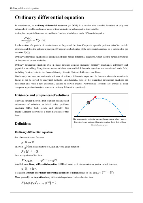
Ordinary differential equationIn mathematics, an ordinary differential equation (or ODE ) is a relation that contains functions of only one independent variable, and one or more of their derivatives with respect to that variable.A simple example is Newton's second law of motion, which leads to the differential equationfor the motion of a particle of constant mass m . In general, the force F depends upon the position x(t) of the particle at time t , and thus the unknown function x(t) appears on both sides of the differential equation, as is indicated in the notation F (x (t )).Ordinary differential equations are distinguished from partial differential equations, which involve partial derivatives of functions of several variables.Ordinary differential equations arise in many different contexts including geometry, mechanics, astronomy and population modelling. Many famous mathematicians have studied differential equations and contributed to the field,including Newton, Leibniz, the Bernoulli family, Riccati, Clairaut, d'Alembert and Euler.Much study has been devoted to the solution of ordinary differential equations. In the case where the equation is linear, it can be solved by analytical methods. Unfortunately, most of the interesting differential equations are non-linear and, with a few exceptions, cannot be solved exactly. Approximate solutions are arrived at using computer approximations (see numerical ordinary differential equations).The trajectory of a projectile launched from a cannon follows a curve determined by an ordinary differential equation that is derived fromNewton's second law.Existence and uniqueness of solutionsThere are several theorems that establish existence anduniqueness of solutions to initial value problemsinvolving ODEs both locally and globally. SeePicard –Lindelöf theorem for a brief discussion of thisissue.DefinitionsOrdinary differential equationLet ybe an unknown function in x with the n th derivative of y , and let Fbe a given functionthen an equation of the formis called an ordinary differential equation (ODE) of order n . If y is an unknown vector valued function,it is called a system of ordinary differential equations of dimension m (in this case, F : ℝmn +1→ ℝm ).More generally, an implicit ordinary differential equation of order nhas the formwhere F : ℝn+2→ ℝ depends on y(n). To distinguish the above case from this one, an equation of the formis called an explicit differential equation.A differential equation not depending on x is called autonomous.A differential equation is said to be linear if F can be written as a linear combination of the derivatives of y together with a constant term, all possibly depending on x:(x) and r(x) continuous functions in x. The function r(x) is called the source term; if r(x)=0 then the linear with aidifferential equation is called homogeneous, otherwise it is called non-homogeneous or inhomogeneous. SolutionsGiven a differential equationa function u: I⊂ R→ R is called the solution or integral curve for F, if u is n-times differentiable on I, andGiven two solutions u: J⊂ R→ R and v: I⊂ R→ R, u is called an extension of v if I⊂ J andA solution which has no extension is called a global solution.A general solution of an n-th order equation is a solution containing n arbitrary variables, corresponding to n constants of integration. A particular solution is derived from the general solution by setting the constants to particular values, often chosen to fulfill set 'initial conditions or boundary conditions'. A singular solution is a solution that can't be derived from the general solution.Reduction to a first order systemAny differential equation of order n can be written as a system of n first-order differential equations. Given an explicit ordinary differential equation of order n (and dimension 1),define a new family of unknown functionsfor i from 1 to n.The original differential equation can be rewritten as the system of differential equations with order 1 and dimension n given bywhich can be written concisely in vector notation aswithandLinear ordinary differential equationsA well understood particular class of differential equations is linear differential equations. We can always reduce an explicit linear differential equation of any order to a system of differential equation of order 1which we can write concisely using matrix and vector notation aswithHomogeneous equationsThe set of solutions for a system of homogeneous linear differential equations of order 1 and dimension nforms an n-dimensional vector space. Given a basis for this vector space , which is called a fundamental system, every solution can be written asThe n × n matrixis called fundamental matrix. In general there is no method to explicitly construct a fundamental system, but if one solution is known d'Alembert reduction can be used to reduce the dimension of the differential equation by one.Nonhomogeneous equationsThe set of solutions for a system of inhomogeneous linear differential equations of order 1 and dimension ncan be constructed by finding the fundamental system to the corresponding homogeneous equation and one particular solution to the inhomogeneous equation. Every solution to nonhomogeneous equation can then be written asA particular solution to the nonhomogeneous equation can be found by the method of undetermined coefficients or the method of variation of parameters.Concerning second order linear ordinary differential equations, it is well known thatSo, if is a solution of: , then such that:So, if is a solution of: ; then a particular solution of , isgiven by:. [1]Fundamental systems for homogeneous equations with constant coefficientsIf a system of homogeneous linear differential equations has constant coefficientsthen we can explicitly construct a fundamental system. The fundamental system can be written as a matrix differential equationwith solution as a matrix exponentialwhich is a fundamental matrix for the original differential equation. To explicitly calculate this expression we first transform A into Jordan normal formand then evaluate the Jordan blocksof J separately asTheories of ODEsSingular solutionsThe theory of singular solutions of ordinary and partial differential equations was a subject of research from the time of Leibniz, but only since the middle of the nineteenth century did it receive special attention. A valuable but little-known work on the subject is that of Houtain (1854). Darboux (starting in 1873) was a leader in the theory, and in the geometric interpretation of these solutions he opened a field which was worked by various writers, notably Casorati and Cayley. To the latter is due (1872) the theory of singular solutions of differential equations of the first order as accepted circa 1900.Reduction to quadraturesThe primitive attempt in dealing with differential equations had in view a reduction to quadratures. As it had been the hope of eighteenth-century algebraists to find a method for solving the general equation of the th degree, so it was the hope of analysts to find a general method for integrating any differential equation. Gauss (1799) showed, however, that the differential equation meets its limitations very soon unless complex numbers are introduced. Hence analysts began to substitute the study of functions, thus opening a new and fertile field. Cauchy was the first to appreciate the importance of this view. Thereafter the real question was to be, not whether a solution is possible by means of known functions or their integrals, but whether a given differential equation suffices for the definition of a function of the independent variable or variables, and if so, what are the characteristic properties of this function.Fuchsian theoryTwo memoirs by Fuchs (Crelle, 1866, 1868), inspired a novel approach, subsequently elaborated by Thomé and Frobenius. Collet was a prominent contributor beginning in 1869, although his method for integrating a non-linear system was communicated to Bertrand in 1868. Clebsch (1873) attacked the theory along lines parallel to those followed in his theory of Abelian integrals. As the latter can be classified according to the properties of the fundamental curve which remains unchanged under a rational transformation, so Clebsch proposed to classify the transcendent functions defined by the differential equations according to the invariant properties of the corresponding surfaces f = 0 under rational one-to-one transformations.Lie's theoryFrom 1870 Sophus Lie's work put the theory of differential equations on a more satisfactory foundation. He showed that the integration theories of the older mathematicians can, by the introduction of what are now called Lie groups, be referred to a common source; and that ordinary differential equations which admit the same infinitesimal transformations present comparable difficulties of integration. He also emphasized the subject of transformations of contact.A general approach to solve DE's uses the symmetry property of differential equations, the continuous infinitesimal transformations of solutions to solutions (Lie theory). Continuous group theory, Lie algebras and differential geometry are used to understand the structure of linear and nonlinear (partial) differential equations for generating integrable equations, to find its Lax pairs, recursion operators, Bäcklund transform and finally finding exact analytic solutions to the DE.Symmetry methods have been recognized to study differential equations arising in mathematics, physics, engineering, and many other disciplines.Sturm–Liouville theorySturm–Liouville theory is a theory of eigenvalues and eigenfunctions of linear operators defined in terms of second-order homogeneous linear equations, and is useful in the analysis of certain partial differential equations.Software for ODE solving•FuncDesigner (free license: BSD, uses Automatic differentiation, also can be used online via Sage-server [2])•VisSim [3] - a visual language for differential equation solving•Mathematical Assistant on Web [4] online solving first order (linear and with separated variables) and second order linear differential equations (with constant coefficients), including intermediate steps in the solution.•DotNumerics: Ordinary Differential Equations for C# and [5] Initial-value problem for nonstiff and stiff ordinary differential equations (explicit Runge-Kutta, implicit Runge-Kutta, Gear’s BDF and Adams-Moulton).•Online experiments with JSXGraph [6]References[1]Polyanin, Andrei D.; Valentin F. Zaitsev (2003). Handbook of Exact Solutions for Ordinary Differential Equations, 2nd. Ed.. Chapman &Hall/CRC. ISBN 1-5848-8297-2.[2]/welcome[3][4]http://user.mendelu.cz/marik/maw/index.php?lang=en&form=ode[5]/NumericalLibraries/DifferentialEquations/[6]http://jsxgraph.uni-bayreuth.de/wiki/index.php/Differential_equationsBibliography• A. D. Polyanin and V. F. Zaitsev, Handbook of Exact Solutions for Ordinary Differential Equations (2nd edition)", Chapman & Hall/CRC Press, Boca Raton, 2003. ISBN 1-58488-297-2• A. D. Polyanin, V. F. Zaitsev, and A. Moussiaux, Handbook of First Order Partial Differential Equations, Taylor & Francis, London, 2002. ISBN 0-415-27267-X• D. Zwillinger, Handbook of Differential Equations (3rd edition), Academic Press, Boston, 1997.•Hartman, Philip, Ordinary Differential Equations, 2nd Ed., Society for Industrial & Applied Math, 2002. ISBN 0-89871-510-5.•W. Johnson, A Treatise on Ordinary and Partial Differential Equations (/cgi/b/bib/ bibperm?q1=abv5010.0001.001), John Wiley and Sons, 1913, in University of Michigan Historical Math Collection (/u/umhistmath/)• E.L. Ince, Ordinary Differential Equations, Dover Publications, 1958, ISBN 0486603490•Witold Hurewicz, Lectures on Ordinary Differential Equations, Dover Publications, ISBN 0-486-49510-8•Ibragimov, Nail H (1993), CRC Handbook of Lie Group Analysis of Differential Equations Vol. 1-3, Providence: CRC-Press, ISBN 0849344883.External links•Differential Equations (/Science/Math/Differential_Equations//) at the Open Directory Project (includes a list of software for solving differential equations).•EqWorld: The World of Mathematical Equations (http://eqworld.ipmnet.ru/index.htm), containing a list of ordinary differential equations with their solutions.•Online Notes / Differential Equations (/classes/de/de.aspx) by Paul Dawkins, Lamar University.•Differential Equations (/diffeq/diffeq.html), S.O.S. Mathematics.• A primer on analytical solution of differential equations (/mws/gen/ 08ode/mws_gen_ode_bck_primer.pdf) from the Holistic Numerical Methods Institute, University of South Florida.•Ordinary Differential Equations and Dynamical Systems (http://www.mat.univie.ac.at/~gerald/ftp/book-ode/ ) lecture notes by Gerald Teschl.•Notes on Diffy Qs: Differential Equations for Engineers (/diffyqs/) An introductory textbook on differential equations by Jiri Lebl of UIUC.Article Sources and Contributors7Article Sources and ContributorsOrdinary differential equation Source: /w/index.php?oldid=433160713 Contributors: 48v, A. di M., Absurdburger, AdamSmithee, After Midnight, Ahadley,Ahoerstemeier,AlfyAlf,Alll,AndreiPolyanin,Anetode,Ap,Arthena,ArthurRubin,BL,BMF81,********************,Bemoeial,BenFrantzDale,Benjamin.friedrich,BereanHunter,Bernhard Bauer, Beve, Bloodshedder, Bo Jacoby, Bogdangiusca, Bryan Derksen, Charles Matthews, Chilti, Chris in denmark, ChrisUK, Christian List, Cloudmichael, Cmdrjameson, Cmprince, Conversion script, Cpuwhiz11, Cutler, Delaszk, Dicklyon, DiegoPG, Dmitrey, Dmr2, DominiqueNC, Dominus, Donludwig, Doradus, Dysprosia, Ed Poor, Ekotkie, Emperorbma, Enochlau, Fintor, Fruge, Fzix info, Gauge, Gene s, Gerbrant, Giftlite, Gombang, HappyCamper, Heuwitt, Hongsichuan, Ht686rg90, Icairns, Isilanes, Iulianu, Jack in the box, Jak86, Jao, JeLuF, Jitse Niesen, Jni, JoanneB, John C PI, Jokes Free4Me, JonMcLoone, Josevellezcaldas, Juansempere, Kawautar, Kdmckale, Krakhan, Kwantus, L-H, LachlanA, Lethe, Linas, Lingwitt, Liquider, Lupo, MarkGallagher,MathMartin, Matusz, Melikamp, Michael Hardy, Mikez, Moskvax, MrOllie, Msh210, Mtness, Niteowlneils, Oleg Alexandrov, Patrick, Paul August, Paul Matthews, PaulTanenbaum, Pdenapo, PenguiN42, Phil Bastian, PizzaMargherita, Pm215, Poor Yorick, Pt, Rasterfahrer, Raven in Orbit, Recentchanges, RedWolf, Rich Farmbrough, Rl, RobHar, Rogper, Romanm, Rpm, Ruakh, Salix alba, Sbyrnes321, Sekky, Shandris, Shirt58, SilverSurfer314, Ssd, Starlight37, Stevertigo, Stw, Susvolans, Sverdrup, Tarquin, Tbsmith, Technopilgrim, Telso, Template namespace initialisation script, The Anome, Tobias Hoevekamp, TomyDuby, TotientDragooned, Tristanreid, Twin Bird, Tyagi, Ulner, Vadimvadim, Waltpohl, Wclxlus, Whommighter, Wideofthemark, WriterHound, Xrchz, Yhkhoo, 今古庸龍, 176 anonymous editsImage Sources, Licenses and ContributorsImage:Parabolic trajectory.svg Source: /w/index.php?title=File:Parabolic_trajectory.svg License: Public Domain Contributors: Oleg AlexandrovLicenseCreative Commons Attribution-Share Alike 3.0 Unported/licenses/by-sa/3.0/。
Some Recent Aspects of Differential Game Theory
Dyn Games Appl(2011)1:74–114DOI10.1007/s13235-010-0005-0Some Recent Aspects of Differential Game TheoryR.Buckdahn·P.Cardaliaguet·M.QuincampoixPublished online:5October2010©Springer-Verlag2010Abstract This survey paper presents some new advances in theoretical aspects of dif-ferential game theory.We particular focus on three topics:differential games with state constraints;backward stochastic differential equations approach to stochastic differential games;differential games with incomplete information.We also address some recent devel-opment in nonzero-sum differential games(analysis of systems of Hamilton–Jacobi equa-tions by conservation laws methods;differential games with a large number of players,i.e., mean-field games)and long-time average of zero-sum differential games.Keywords Differential game·Viscosity solution·System of Hamilton–Jacobi equations·Mean-field games·State-constraints·Backward stochastic differential equations·Incomplete information1IntroductionThis survey paper presents some recent results in differential game theory.In order to keep the presentation at a reasonable size,we have chosen to describe in full details three topics with which we are particularly familiar,and to give a brief summary of some other research directions.Although this choice does not claim to represent all the recent literature on the R.Buckdahn·M.QuincampoixUniversitéde Brest,Laboratoire de Mathématiques,UMR6205,6Av.Le Gorgeu,BP809,29285Brest, FranceR.Buckdahne-mail:Rainer.Buckdahn@univ-brest.frM.Quincampoixe-mail:Marc.Quincampoix@univ-brest.frP.Cardaliaguet( )Ceremade,UniversitéParis-Dauphine,Place du Maréchal de Lattre de Tassigny,75775Paris Cedex16, Francee-mail:cardaliaguet@ceremade.dauphine.frmore theoretic aspects of differential game theory,we are pretty much confident that it cov-ers a large part of what has recently been written on the subject.It is clear however that the respective part dedicated to each topic is just proportional to our own interest in it,and not to its importance in the literature.The three main topics we have chosen to present in detail are:–Differential games with state constraints,–Backward stochastic differential equation approach to differential games,–Differential games with incomplete information.Before this,we also present more briefly two domains which have been the object of very active research in recent years:–nonzero-sum differential games,–long-time average of differential games.Thefirst section of this survey is dedicated to nonzero-sum differential games.Although zero-sum differential games have attracted a lot of attention in the80–90’s(in particular, thanks to the introduction of viscosity solutions for Hamilton–Jacobi equations),the ad-vances on nonzero-sum differential games have been scarcer,and mainly restricted to linear-quadratic games or stochastic differential games with a nondegenerate diffusion.The main reason for this is that there was very little understanding of the system of Hamilton–Jacobi equations naturally attached to these games.In the recent years the analysis of this sys-tem has been the object of several papers by Bressan and his co-authors.At the same time, nonzero-sum differential games with a very large number of players have been investigated in the terminology of mean-field games by Lasry and Lions.In the second section we briefly sum up some advances in the analysis of the large time behavior of zero-sum differential games.Such problems have been the aim of intense re-search activities in the framework of repeated game theory;it has however only been re-cently investigated for differential games.In the third part of this survey(thefirst one to be the object of a longer development) we investigate the problem of state constraints for differential games,and in particular,for pursuit-evasion games.Even if such class of games has been studied since Isaacs’pioneer-ing work[80],the existence of a value was not known up to recently for these games in a rather general framework.This is mostly due to the lack of regularity of the Hamiltonian and of the value function,which prevents the usual viscosity solution approach to work(Evans and Souganidis[63]):Indeed some controllability conditions on the phase space have to be added in order to prove the existence of the value(Bardi,Koike and Soravia[18]).Following Cardaliaguet,Quincampoix and Saint Pierre[50]and Bettiol,Cardaliaguet and Quincam-poix[26]we explain that,even without controllability conditions,the game has a value and that this value can be characterized as the smallest supersolution of some Hamilton–Jacobi equation with discontinuous Hamiltonian.Next we turn to zero-sum stochastic differential games.Since the pioneering work by Fleming and Souginidis[65]it has been known that such games have a value,at least in a framework of games of the type“nonanticipating strategies against controls”.Unfortunately this notion of strategies is not completely satisfactory,since it presupposes that the players have a full knowledge of their opponent’s control in all states of the world:It would be more natural to assume that the players use strategies which give an answer to the control effectively played by their opponent.On the other hand it seems also natural to consider nonlinear cost functionals and to allow the controls of the players to depend on events of the past which happened before the beginning of the game.The last two points have beeninvestigated in a series of papers by Buckdahn and Li[35,36,39],and an approach more direct than that in[65]has been developed.Thefirst point,together with the two others,will be the object of the fourth part of the survey.In the last part we study differential games with incomplete information.In such games, one of the parameters of the game is chosen at random according to some probability mea-sure and the result is told to one of the players and not to the other.Then the game is played as usual,players observing each other’s control.The main difference with the usual case is that at least one of the players does not know which payoff he is actually optimizing.All the difficulty of this game is to understand what kind of information the informed player has interest in to disclose in order to optimize his payoff,taking thus the risk that his opponent learns his missing information.Such games are the natural extension to differential games of the Aumann–Maschler theory for repeated games[11].Their analysis has been developed in a series of papers by Cardaliaguet[41,43–45]and Cardaliaguet and Rainer[51,52].Throughout these notes we assume the reader to be familiar with the basic results of dif-ferential game theory.Many references can be quoted on this subject:A general introduction for the formal relation between differential games and Hamilton–Jacobi equations(or sys-tem)can be found in the monograph Baçar and Olsder[13].We also refer the reader to the classical monographs by Isaacs[80],Friedman[67]and Krasovskii and Subbotin[83]for early presentations of differential game theory.The recent literature on differential games strongly relies on the notion of viscosity solution:Classical monographs on this subject are Bardi and Capuzzo Dolcetta[17],Barles[19],Fleming and Soner[64],Lions[93]and the survey paper by Crandall,Ishii and Lions[56].In particular[17]contains a good introduc-tion to the viscosity solution aspects of deterministic zero-sum differential games:the proof of the existence and the characterization of a value for a large class of differential games can be found there.Section6is mostly based on the notion of backward stochastic differential equation(BSDE):We refer to El Karoui and Mazliak[60],Ma and Yong[96]and Yong and Zhou[116]for a general presentation.The reader is in particular referred to the work by S.Peng on BSDE methods in stochastic control[101].Let usfinally note that,even if this survey tries to cover a large part of the recent literature on the more theoretical aspects of differential games,we have been obliged to omit some topics:linear-quadratic differential games are not covered by this survey despite their usefulness in applications;however,these games have been already the object of several survey ck of place also prevented us from describing advances in the domain of Dynkin games.2Nonzero-sum Differential GamesIn the recent years,the more striking advances in the analysis of nonzero-sum differential games have been directed in two directions:analysis by P.D.E.methods of Nash feedback equilibria for deterministic differential games;differential games with a very large number of small players(mean-field games).These topics appear as the natural extensions of older results:existence of Nash equilibria in memory strategies and of Nash equilibria in feedback strategies for stochastic differential games,which have also been revisited.2.1Nash Equilibria in Memory StrategiesSince the work of Kononenko[82](see also Kleimenov[81],Tolwinski,Haurie and Leit-mann[114],Gaitsgory and Nitzan[68],Coulomb and Gaitsgory[55]),it has been knownthat deterministic nonzero-sum differential games admit Nash equilibrium payoffs in mem-ory strategies:This result is actually the counterpart of the so-called Folk Theorem in re-peated game theory[100].Recall that a memory(or a nonanticipating)strategy for a player is a strategy where this player takes into account the past controls played by the other play-ers.In contrast a feedback strategy is a strategy which only takes into account the present position of the system.Following[82]Nash equilibrium payoffs in memory strategies are characterized as follows:A payoff is a Nash equilibrium payoff if and only if it is reach-able(i.e.,the players can obtain it by playing some control)and individually rational(the expected payoff for a player lies above its min-max level at any point of the resulting trajec-tory).This result has been recently generalized to stochastic differential games by Buckdahn, Cardaliaguet and Rainer[38](see also Rainer[105])and to games in which players can play random strategies by Souquière[111].2.2Nash Equilibria in Feedback FormAlthough the existence and characterization result of Nash equilibrium payoffs in mem-ory strategies is quite general,it has several major drawbacks.Firstly,there are,in general, infinitely many such Nash equilibria,but there exists—at least up to now—no completely satisfactory way to select one.Secondly,such equilibria are usually based on threatening strategies which are often non credible.Thirdly,the corresponding strategies are,in general, not“time-consistent”and in particular cannot be computed by any kind of“backward in-duction”.For this reason it is desirable tofind more robust notions of Nash equilibria.The best concept at hand is the notion of subgame perfect Nash equilibria.Since the works of Case[54]and Friedman[67],it is known that subgame perfect Nash equilibria are(at least heuristically)given by feedback strategies and that their corresponding payoffs should be the solution of a system of Hamilton–Jacobi equations.Up to now these ideas have been successfully applied to linear-quadratic differential games(Case[54],Starr and Ho[113], ...)and to stochastic differential games with non degenerate viscosity term:In thefirst case,one seeks solutions which are quadratic with respect to the state variable;this leads to the resolution of Riccati equations.In the latter case,the regularizing effect of the non-degenerate diffusion allows us to usefixed point arguments to get either Nash equilibrium payoffs or Nash equilibrium feedbacks.Several approaches have been developed:Borkar and Ghosh[27]consider infinite horizon problems and use the smoothness of the invari-ant measure associated to the S.D.E;Bensoussan and Frehse[21,22]and Mannucci[97] build“regular”Nash equilibrium payoffs satisfying a system of Hamilton–Jacobi equations thanks to elliptic or parabolic P.D.E techniques;Nash equilibrium feedbacks can also be built by backward stochastic differential equations methods like in Hamadène,Lepeltier and Peng[75],Hamadène[74],Lepeltier,Wu and Yu[92].2.3Ill-posedness of the System of HJ EquationsIn a series of articles,Bressan and his co-authors(Bressan and Chen[33,34],Bressan and Priuli[32],Bressan[30,31])have analyzed with the help of P.D.E methods the system of Hamilton–Jacobi equations arising in the construction of feedback Nash equilibria for deter-ministic nonzero-sum games.In state-space dimension1and for thefinite horizon problem, this system takes the form∂V i+H i(x,D V1,...,D V n)=0in R×(0,T),i=1,...,n,coupled with a terminal condition at time T(here n is the number of players and H i is the Hamiltonian of player i,V i(t,x)is the payoff obtained by player i for the initial condition (t,x)).Setting p i=(V i)x and deriving the above system with respect to x one obtains the system of conservation laws:∂t p i+H i(x,p1,...,p n)x=0in R×(0,T).This system turns out to be,in general,ill-posed.Typically,in the case of two players(n= 2),the system is ill-posed if the terminal payoff of the players have an opposite monotonicity. If,on the contrary,these payoffs have the same monotony and are close to some linear payoff (which is a kind of cooperative case),then the above system has a unique solution,and one can build Nash equilibria in feedback form from the solution of the P.D.E[33].Still in space dimension1,the case of infinite horizon seems more promising:The sys-tem of P.D.E then reduces to an ordinary differential equation.The existence of suitable solutions for this equation then leads to Nash equilibria.Such a construction is carried out in Bressan and Priuli[32],Bressan[30,31]through several classes of examples and by various methods.In a similar spirit,the papers Cardaliaguet and Plaskacz[47],Cardaliaguet[42]study a very simple class of nonzero-sum differential games in dimension1and with a terminal payoff:In this case it is possible to select a unique Nash equilibrium payoff in feedback form by just imposing that it is Pareto whenever there is a unique Pareto one.However,this equilibrium payoff turns out to be highly unstable with respect to the terminal data.Some other examples of nonlinear-quadratic differential games are also analyzed in Olsder[99] and in Ramasubramanian[106].2.4Mean-field GamesSince the system of P.D.Es arising in nonzero-sum differential games is,in general,ill-posed,it is natural to investigate situations where the problem simplifies.It turns out that this is the case for differential games with a very large number of identical players.This problem has been recently developed in a series of papers by Lasry and Lions[87–90,94] under the terminology of mean-field games(see also Huang,Caines and Malhame[76–79] for a related approach).The main achievement of Lasry and Lions is the identification of the limit when the number of players tends to infinity.The typical resulting model takes the form⎧⎪⎨⎪⎩(i)−∂t u−Δu+H(x,m,Du)=0in R d×(0,T),(ii)∂t m−Δm−divD p H(x,m,Du)m=0in R d×(0,T),(iii)m(0)=m0,u(x,T)=Gx,m(T).(1)In the above system,thefirst equation has to be understood backward in time while the second one is forward in time.Thefirst equation(a Hamilton–Jacobi one)is associated with an optimal control problem and its solution can be regarded as the value function for a typical small player(in particular the Hamiltonian H=H(x,m,p)is convex with respect to the last variable).As for the second equation,it describes the evolution of the density m(t)of the population.More precisely,let usfirst consider the behavior of a typical player.He controls through his control(αs)the stochastic differential equationdX t=αt dt+√2B t(where(B t)is a standard Brownian motion)and he aims at minimizing the quantityET12LX s,m(s),αsds+GX T,m(T),where L is the Fenchel conjugate of H with respect to the p variable.Note that in this cost the evolving measure m(s)enters as a parameter.The value function of our average player is then given by(1-(i)).His optimal control is—at least heuristically—given in feedback form byα∗(x,t)=−D p H(x,m,Du).Now,if all agents argue in this way,their repartition will move with a velocity which is due,on the one hand,to the diffusion,and,one the other hand,to the drift term−D p H(x,m,Du).This leads to the Kolmogorov equation(1-(ii)).The mean-field game theory developed so far has been focused on two main issues:firstly,investigate equations of the form(1)and give an interpretation(in economics,for instance)of such systems.Secondly,analyze differential games with afinite but large num-ber of players and interpret(1)as their limiting behavior as the number of players goes to infinity.Up to now thefirst issue is well understood and well documented.The original works by Lasry and Lions give a certain number of conditions under which(1)has a solution,discuss its uniqueness and its stability.Several papers also study the numerical approximation of this solution:see Achdou and Capuzzo Dolcetta[1],Achdou,Camilli and Capuzzo Dolcetta[2], Gomes,Mohr and Souza[71],Lachapelle,Salomon and Turinici[85].The mean-field games theory has been used in the analysis of wireless communication systems in Huang,Caines and Malhamé[76],or Yin,Mehta,Meyn and Shanbhag[115].It seems also particularly adapted to modeling problems in economics:see Guéant[72,73],Lachapelle[84],Lasry, Lions,Guéant[91],and the references therein.As for the second part of the program,the limiting behavior of differential games when the number of players tend to infinity has been understood for ergodic differential games[88].The general case remains mostly open.3Long-time Average of Differential GamesAnother way to reduce the complexity of differential games is to look at their long-time be-havior.Among the numerous applications of this topic let us quote homogenization,singular perturbations and dimension reduction of multiscale systems.In order to explain the basic ideas,let us consider a two-player stochastic zero-sum dif-ferential game with dynamics given bydX t,ζ;u,vs =bX t,ζ;u,vs,u s,v sds+σX t,ζ;u,v,u s,v sdB s,s∈[t,+∞),X t=ζ,where B is a d-dimensional standard Brownian motion on a given probability space (Ω,F,P),b:R N×U×V→R N andσ:R N×U×V→R N×d,U and V being some metric compact sets.We assume that thefirst player,playing with u,aims at minimizing a running payoff :R N×U×V→R(while the second players,playing with v,maximizes). Then it is known that,under some Isaacs’assumption,the game has a value V T which is the viscosity solution of a second order Hamilton–Jacobi equation of the form−∂t V T(t,x)+Hx,D V T(t,x),D2V T(t,x)=0in[0,T]×R N,V T(T,x)=0in R N.A natural question is the behavior of V T as T→+∞.Actually,since V T is typically of linear growth,the natural quantity to consider is the long-time average,i.e.,lim T→+∞V T/T.Interesting phenomena can be observed under some compactness assumption on the un-derlying state-space.Let us assume,for instance,that the maps b(·,u,v),σ(·,u,v)and (·,u,v)are periodic in all space variables:this actually means that the game takes place in the torus R N/Z N.In this framework,the long-time average is well understood in two cases:either the dif-fusion is strongly nondegenerate:∃ν>0,(σσ∗)(x,u,v)≥νI N∀x,u,v,(where the inequality is understood in the sense of quadratic matrices);orσ≡0and H= H(x,ξ)is coercive:lim|ξ|→+∞H(x,ξ)=+∞uniformly with respect to x.(2) In both cases the quantity V T(x,0)/T uniformly converges to the unique constant¯c forwhich the problem¯c+Hx,Dχ(x),D2χ(x)=0in R Nhas a continuous,periodic solutionχ.In particular,the limit is independent of the initial condition.Such kind of results has been proved by Lions,Papanicoulaou and Varadhan[95] forfirst order equations(i.e.,deterministic differential games).For second order equations, the result has been obtained by Alvarez and Bardi in[3],where the authors combine funda-mental contributions of Evans[61,62]and of Arisawa and Lions[7](see also Alvarez and Bardi[4,5],Bettiol[24],Ghosh and Rao[70]).For deterministic differential games(i.e.,σ≡0),the coercivity condition(2)is not very natural:Indeed,it means that one of the players is much more powerful than the other one. However,very little is known without such a condition.Existing results rely on a specific structure of the game:see for instance Bardi[16],Cardaliaguet[46].The difficulty comes from the fact that,in these cases,the limit may depend upon the initial condition(see also Arisawa and Lions[7],Quincampoix and Renault[104]for related issues in a control set-ting).The existence of a limit for large time differential games is certainly one of the main challenges in differential games theory.4Existence of a Value for Zero-sum Differential Games with State Constraints Differential games with state constraints have been considered since the early theory of differential games:we refer to[23,28,66,69,80]for the computation of the solution for several examples of pursuit.We present here recent trends for obtaining the existence of a value for a rather general class of differential games with constraints.This question had been unsolved during a rather long period due to problems we discuss now.The main conceptual difficulty for considering such zero-sum games lies in the fact that players have to achieve their own goal and to satisfy the state constraint.Indeed,it is not clear to decide which players has to be penalized if the state constraint is violated.For this reason,we only consider a specific class of decoupled games where each player controls independently a part of the dynamics.A second mathematical difficulty comes from the fact that players have to use admissible controls i.e.,controls ensuring the trajectory to fulfilthe state constraint.A byproduct of this problem is the fact that starting from two close initial points it is not obvious tofind two close constrained trajectories.This also affects the regularity of value functions associated with admissible controls:The value functions are,in general,not Lipschitz continuous anymore and,consequently,classical viscosity solutions methods for Hamilton–Jacobi equations may fail.4.1Statement of the ProblemWe consider a differential game where thefirst player playing with u,controls afirst systemy (t)=gy(t),u(t),u(t)∈U,y(t0)=y0∈K U,(3) while the second player,playing with v,controls a second systemz (t)=hz(t),v(t),v(t)∈V,z(t0)=z0∈K V.(4)For every time t,thefirst player has to ensure the state constraint y(t)∈K U while the second player has to respect the state constraint z(t)∈K V for any t∈[t0,T].We denote by x(t)= x[t0,x0;u(·),v(·)](t)=(y[t0,y0;u(·)](t),z[t0,z0;v(·)](t))the solution of the systems(3) and(4)associated with an initial data(t0,x0):=(t0,y0,z0)and with a couple of controls (u(·),v(·)).In the following lines we summarize all the assumptions concerning with the vectorfields of the dynamics:⎧⎪⎪⎪⎪⎪⎪⎪⎪⎪⎪⎪⎪⎪⎪⎪⎪⎪⎪⎪⎪⎪⎪⎪⎨⎪⎪⎪⎪⎪⎪⎪⎪⎪⎪⎪⎪⎪⎪⎪⎪⎪⎪⎪⎪⎪⎪⎪⎩(i)U and V are compact subsets of somefinitedimensional spaces(ii)f:R n×U×V→R n is continuous andLipschitz continuous(with Lipschitz constant M)with respect to x∈R n(iii)uf(x,u,v)andvf(x,u,v)are convex for any x(iv)K U={y∈R l,φU(y)≤0}withφU∈C2(R l;R),∇φU(y)=0ifφU(y)=0(v)K V={z∈R m,φV(z)≤0}withφV∈C2(R m;R),∇φV(z)=0ifφV(z)=0(vi)∀y∈∂K U,∃u∈U such that ∇φU(y),g(y,u) <0(vii)∀z∈∂K V,∃v∈V such that ∇φV(z),h(z,v) <0(5)We need to introduce the notion of admissible controls:∀y0∈K U,∀z0∈K V and∀t0∈[0,T]we defineU(t0,y0):=u(·):[t0,+∞)→U measurable|y[t0,y0;u(·)](t)∈K U∀t≥t0V(t0,z0):=v(·):[t0,+∞)→V measurable|z[t0,z0;v(·)](t)∈K V∀t≥t0.Under assumptions(5),the Viability Theorem(see[9,10])ensures that for all x0= (y0,z0)∈K U×K VU(t0,y0)=∅and V(t0,z0)=∅.Throughout the paper we omit t0in the notations U(t0,y0)and U(t0,y0)whenever t0=0.We now describe two quantitative differential games.Let us start with a game with an integral cost:Bolza Type Differential Game Given a running cost L:[0,T]×R N×U×V→R and afinal costΨ:R N→R,we define the payoff associated to an initial position(t0,x0)= (t0,y0,z0)and to a pair of controls(u,v)∈U(t0,y0)×V(t0,z0)byJt0,x0;u(·),v(·)=Tt0Lt,x(t),u(·),v(·)dt+Ψx(T),(6)where x(t)=x[t0,x0;u(·),v(·)](t)=(y[t0,y0;u(·)](t),z[t0,z0;v(·)](t))denotes the solu-tion of the systems(3)and(4).Thefirst player wants to maximize the functional J,while the second player’s goal is to minimize J.Definition1A mapα:V(t0,z0)→U(t0,y0)is a nonanticipating strategy(for thefirst player and for the point(t0,x0):=(t0,y0,z0)∈R+×K U×K V)if,for anyτ>0,for all controls v1(·)and v2(·)belonging to V(t0,z0),which coincide a.e.on[t0,t0+τ],α(v1(·)) andα(v2(·))coincide almost everywhere on[t0,t0+τ].Nonanticipating strategiesβfor the second player are symmetrically defined.For any point x0∈K U×K V and∀t0∈[0,T]we denote by A(t0,x0)and by B(t0,x0)the sets of the nonanticipating strategies for thefirst and the second player respectively.We are now ready to define the value functions of the game.The lower value V−is defined by:V−(t0,x0):=infβ∈B(t0,x0)supu(·)∈U(t0,y0)Jt0,x0;u(·),βu(·),(7)where J is defined by(6).On the other hand we define the upper value function as follows:V+(t0,x0):=limε→0+supα∈A(t0,x0)infv(·)∈V(t0,z0)Jεt0,x0;αv(·),v(·)(8)withJεt0,x0;u(·),v(·):=Tt0Lt,x(t),u(t),v(t)dt+Ψεx(T),where x(t)=x[t0,x0;u(·),v(·)](t)andΨεis the lower semicontinuous function defined byΨε(x):=infρ∈R|∃y∈R n with(y,ρ)−x,Ψ(x)=ε.The asymmetry between the definition of the value functions is due to the fact that one assumes that the terminal payoffΨis lower semicontinuous.WhenΨis continuous,one can check that V+can equivalently be defined in a more natural way asV+(t0,x0):=supα∈A(t0,x0)infv(·)∈V(t0,z0)Jt0,x0;αv(·),v(·).We now describe the second differential game which is a pursuit game with closed target C⊂K U×K V.Pursuit Type Differential Game The hitting time of C for a trajectory x(·):=(y(·),z(·)) is:θCx(·):=inft≥0|x(t)∈C.If x(t)/∈C for every t≥0,then we setθC(x(·)):=+∞.In the pursuit game,thefirst player wants to maximizeθC while the second player wants to minimize it.The value functions aredefined as follows:The lower optimal hitting-time function is the mapϑ−C :K U×K V→R+∪{+∞}defined,for any x0:=(y0,z0),byϑ−C (x0):=infβ(·)∈B(x0)supu(·)∈U(y0)θCxx0,u(·),βu(·).The upper optimal hitting-time function is the mapϑ+C :K U×K V→R+∪{+∞}de-fined,for any x0:=(y0,z0),byϑ+ C (x0):=limε→0+supα(·)∈A(x0)infv(·)∈V(z0)θC+εBxx0,αv(·),v(·).By convention,we setϑ−C (x)=ϑ+C(x)=0on C.Remarks–Note that here again the definition of the upper and lower value functions are not sym-metric:this is related to the fact that the target assumed to be closed,so that the game is intrinsically asymmetric.–The typical pursuit game is the case when the target coincides with the diagonal:C= {(y,z),|y=z}.We refer the reader to[6,29]for various types of pursuit games.The formalism of the present survey is adapted from[50].4.2Main ResultThe main difficulty for the analysis of state-constraint problems lies in the fact that two trajectories of a control system starting from two—close—different initial conditions could be estimated by classical arguments on the continuity of theflow of the differential equation. For constrained systems,it is easy to imagine cases where the constrained trajectories starting from two close initial conditions are rather far from each other.So,an important problem in order to get suitable estimates on constrained trajectories,is to obtain a kind of Filippov Theorem with ly a result which allows one to approach—in a suitable sense—a given trajectory of the dynamics by a constrained trajectory.Note that similar results exist in the literature.However,we need here to construct a constrained trajectory in a nonanticipating way[26](cf.also[25]),which is not the case in the previous constructions.Proposition1Assume that conditions(5)are satisfied.For any R>0there exist C0= C0(R)>0such that for any initial time t0∈[0,T],for any y0,y1∈K U with|y0|,|y1|≤R,。
- 1、下载文档前请自行甄别文档内容的完整性,平台不提供额外的编辑、内容补充、找答案等附加服务。
- 2、"仅部分预览"的文档,不可在线预览部分如存在完整性等问题,可反馈申请退款(可完整预览的文档不适用该条件!)。
- 3、如文档侵犯您的权益,请联系客服反馈,我们会尽快为您处理(人工客服工作时间:9:00-18:30)。
a rX iv:mat h /45471v2[mat h.CV]26J u l24Differentiable functions of Cayley-Dickson numbers.S.V.Ludkovsky.27.05.2004Abstract We investigate superdifferentiability of functions defined on regions of the real octonion (Cayley)algebra and obtain a noncommutative version of the Cauchy-Riemann conditions.Then we study the non-commutative analog of the Cauchy integral as well as criteria for func-tions of an octonion variable to be analytic.In particular,the octonion exponential and logarithmic functions are being considered.Moreover,superdifferentiable functions of variables belonging to Cayley-Dickson algebras (containing the octonion algebra as the proper subalgebra)finite and infinite dimensional are investigated.Among main results there are the Cayley-Dickson algebras analogs of Caychy’s theorem,Hurtwitz’,argument principle,Mittag-Leffler’s,Rouche’s and Weier-strass’theorems.1Introduction Functions of real variables with values in Clifford algebras were investigated,for example,in [5].In this article we continue our investigations of functions of variables belonging to noncommutative superalgebras [27]considering here functions of octonion variables and also of more general Cayley-Dickson al-gebras A r ,r ≥4,containing the octonion algebra as the proper subalge-bra.The algebra of octonions is alternative,that gives possibility to define residues of functions in a reasonable way.The Cayley-Dickson algebras of larger dimensions are not already alternative and proceedings for them are1heavier.Nevertheless,using their power-associativity and distributivity it is possible to define differentiability of functions of variables belonging to the Cayley-Dickson algebra such that the differential has sufficiently well prop-erties,that to define subsequently the line integral over such variable.This integral is extended on spaces of continuous functions along rectifiable paths. It is necessary to note,that the graded structure of the Cayley-Dickson alge-bra A r over R and its noncommutativity for the real dimension not less,than 4causes well properites of superdifferentiable functions f:U→A r,where U is open in A n r.Apart from the complex case a derivative f′of f∈C1(U,A r) is an operator and not in general a number even for U⊂A r,n=1.The theory of A r-holomorphic functions given below can not be reduced to the theory of holomorphic functions of several complex variables.More-over,A r-holomorphic functions have many specific features in comparison with real locally analytic functions as,for example,the argument princi-ple,homotopy theorem2.15,theorem about representations of multiples of functions with the help of line integral along a loop,etc.show.Dirac had used biquaternions(complexified quaternions)in his investiga-tions of quantum mechanics.The Dirac equations D z f1−D˜z f2=m(f1+f2) and D˜z f1+D z f2=m(f1−f2)on the space of right superlinearly(z,˜z)-superdifferentiable functions of quaternion variable can be extended on the space of(z,˜z)-superdifferentiable functions f1(z,˜z)and f2(z,˜z)(see our def-inition in§2.2below and in[27])gives evident physical interpretation of a solution(f1,f2),r≥2,as spinors,where m is a mass of an elementary parti-cle.We extend the operator(D2z+D2˜z)from the space of right superlinearly (z,˜z)-superdifferentiable functions on the space of(z,˜z)-superdifferentiable functions f,hence we get the Klein-Gordon equation(D2z+D2˜z)f=2m2f in the particular case of quaternions and A r-algebras,r≥3.It is necessary to note that previous authors have used right(or left)superlinearly superdiffer-entiable functions,that does not form an algebra of functions and they have used multiple and iterated integrals and the Gauss-Ostrogradskii-Green for-mula,but they have not used line integrals over A r(see,for example,[11]and references therein).While development their theory Yang and Mills known in theoretical and mathematical physics had actively worked with quater-nions,but they have felt lack of the available theory of quaternion functions existing in their time.Yang also have expressed the idea,that possibly in quantumfield theory it is worthwhile to use quaternion time(see page198 [11]).It is known also the use of complex time through the Wick rotation in2quantum mechanics for getting solutions of problems,where the imaginary time is used for interpretations of probabilities of tunneling under energy barriers(walls).Using the special unitary group embedded into the quater-nion skewfield H it makes equivalent under isomoprphism with SO(3)all spatial axes.On the other hand,the major instrument for measurement is the spectrum.When there are deep energy wells or high energy walls,then it makes obstacles for penetrating electromagnetic waves and radiation,that is well known also in astronomy,where black holes are actively studied(see page199and§3.b[11]and references therein).W.Hamilton in his lectures on quaternions also tackled a question of events in H and had thought about use of quaternions in astronomy and celestial mechanics(see[12,30]and references therein).Therefore,in general to compare the sequence of events it may be necessary in definite situations to have the same dimensional time space as the coordinate space.On the other hand,spatial isotropy at least local in definite domains makes from each axis under rotations and dilata-tions SU(2)×R isomorphic with H.Therefeore,it appears that in definite situations it would be sufficent to use H4instead of the Minkowski space-time R1,3,where R1,3has the embedding into H.Since H as the R-linear space is isomorphic with R4,then there exists the embeddingζof R1,3into H such thatζ(x1,x i,x j,x k)=x1+x i i+x j j+x k k,where the R1,3-norm is given by the equation|x|1,3=(x2+˜x2)/2=Re(x2)=x21−x2i−x2j−x2k and the R1,3scalar product is given by the equality(x,y)1,3:=(xy+˜y˜x)/2=Re(xy) =x1y1−x i y i−x j y j−x k y k,where x=x1+x i i+x j j+x k k,x1,...,x k∈R (see§2.1).This also can be used for embeddings of hyperbolic manifolds into quaternion manifolds.Then H4can be embedded into the algebra A4 of sedenions.It is also natural for describing systems with spin,isospin,flavor,color and their interactions.The enlargement of the space-time also is dictated in some situations by symmetry properties of differential equa-tions or a set of operators describing a system.For example,special uni-tary groups SU(n),for n=3,5−8,11,etc.,exceptional Lie groups,are actively used in theory of elementary particles[11],but these groups can be embedded into the corresponding Cayley-Dickson algebra A r[1].In-deed,U(m)⊂GL(n,C)⊂C n2while C m has the embedding into A r, where m=2r−1,such that C m∋(x1+iy1,...,x m+iy m)=:ξ→z:= (x1+i1y1)+i2(x2+i∗2i3y2)+...+i2m−2(x m+i∗2m−2i2m−1y m)∈A r,since (i∗l i k)2=−1for each l=k≥1,where{i0,i1,...,i2m−1}is the basis of gen-erators of A r,i0=1,i2k=−1,i0i k=i k i0,i l i k=−i k i l for each k=l≥1,3i=(−1)1/2,z∗=x1−i1y1−i2x2−i3y2−...−i2m−2x m−i2m−1y m,the norm (zz∗)1/2=:|z|=( m k=1|x k+iy k|2)1/2=:|ξ|satisfies the parallelogramm identity and induces the scalar product.This paper as the previous one[27]is devoted to the solution of the W.Hamilton problem of developing line integral and holomorphic function theory of quaternion variables,but now we consider general case of Cayley-Dickson algebras variables.In this paper we investigate differentiability of functions defined on re-gions of the real octonion(Cayley)algebra.For this we consider specific definition of superdifferentiability and obtain a noncommutative version of the Cauchy-Riemann conditions in the particular case of right superlinear superdifferentiability.Then we study the noncommutative analog of the Cauchy integral as well as criteria for functions of an octonion variable to be analytic.In particular,the octonion exponential and logarithmic func-tions are being considered.Moreover,superdifferentiable functions of vari-ables belonging to Cayley-Dickson algebras(containing the octonion algebra as the proper subalgebra)finite and infinite dimensional are investigated. Among main results there are the Cayley-Dickson algebras analogs of Cay-chy’s theorem,Hurtwitz’,argument principle,Mittag-Leffler’s,Rouche’s and Weierstrass’theorems.The results of this paper can serve for subsequent investigations of special functions of Cayley-Dickson algebra variables,noncommutative sheaf theory, manifolds of noncommutative geometry over Cayley-Dickson algebras,their groups of loops and diffeomorphisms(see also[23,24,25,26,29]).2Differentiability of functions of octonion vari-ablesTo avoid misunderstandings wefirst introduce notations.2.1.We write H for the skewfield of quaternions over the realfield R with the classical quaternion basis1,i,j,k,satisfying relations of A2(see Introduction).The quaternion skewfield H has an anti-automorphismηof order twoη:z→˜z,where˜z=w1−w i i−w j j−w k k,z=w1+w i i+w j j+w k k;w1,...,w k∈R.There is a norm in H such that|z|=|z˜z|1/2,hence˜z=|z|2z−1.4The algebra K of octonions(octaves,the Cayley algebra)is defined as an eight-dimensional algebra over R with a basis,for example,(1)b3:=b:={1,i,j,k,l,il,jl,kl}such that(2)i2=j2=k2=l2=−1,ij=k,ji=−k,jk=i,kj=−i,ki=j, ik=−j,li=−il,jl=−lj,kl=−lk;(3)(α+βl)(γ+δl)=(αγ−˜δβ)+(δα+β˜γ)lis the multiplication law in K for eachα,β,γ,δ∈H,ξ:=α+βl∈K,η:=γ+δl∈K,˜z:=v−wi−xj−yk for a quaternion z=v+wi+xj+yk∈H with v,w,x,y∈R.The octonion algebra is neither commutative,nor associative,since(ij)l= kl,i(jl)=−kl,but it is distributive and R1is its center.Ifξ:=α+βl∈K, then(4)˜ξ:=˜α−βl is called the adjoint element ofξ,whereα,β∈H.Then(5)(ξη)˜.=˜η˜ξ,˜ξ+˜η=(ξ+η)˜.andξ˜ξ=|α|2+|β|2,where|α|2=α˜αsuch that(6)ξ˜ξ=:|ξ|2and|ξ|is the norm in K.Therefore,(7)|ξη|=|ξ||η|,consequently,K does not contain divisors of zero(see also[17,21,35]).The multiplication of octonions satsifies equations:(8)(ξη)η=ξ(ηη),(9)ξ(ξη)=(ξξ)η,that forms the alternative system.In particular,(ξξ)ξ=ξ(ξξ).Put˜ξ= 2a−ξ,where a=Re(ξ):=(ξ+˜ξ)/2∈R.Since R1is the center of K and˜ξξ=ξ˜ξ=|ξ|2,then from(8,9)by induction it follows,that for each ξ∈K and each n-tuplet(product),n∈N,ξ(ξ(...ξξ)...)=(...(ξξ)ξ...)ξthe result does not depend on an order of brackets(order of consequtive multiplications),hence the definition ofξn:=ξ(ξ(...ξξ)...)does not depend on the order of brackets.This also shows thatξmξn=ξnξm,ξm˜ξm=˜ξmξn for each n,m∈N andξ∈K.Apart from the quaternions,the octonion algebra can not be realized as the subalgebra of the algebra M8(R)of all 8×8-matrices over R,since K is not associative,but M8(R)is associative. The noncommutative nonassociative octonion algebra K is the Z2-graded R-algebra K=K0+K1,where elements of K0are even(see,for example,[20,21,34]).There are the natural embeddings C֒→K and H֒→K,but neither K over C,nor K over H,nor H over C are algebras,since the centres of them are Z(H)=Z(K)=R.We consider also the Cayley-Dickson algebras A n over R,where2n is its5dimension over R.They are constructed by induction starting from R such that A n+1is obtained from A n with the help of the doubling procedure,in particular,A0:=R,A1=C,A2=H,A3=K and A4is known as the sedenion algebra[1].The Cayley-Dickson algebras are∗-algebras,that is, there is a real-linear mapping A n∋a→a∗∈A n such that(10)a∗∗=a,(11)(ab)∗=b∗a∗for each a,b∈A n.Then they are nicely normed,that is,(12)a+a∗=:2Re(a)∈R and(13)aa∗=a∗a>0for each0=a∈A n.The norm in it is defined by(14)|a|2:=aa∗.We also denote a∗by˜a.Each0=a∈A n has a multiplicative inverse given by a−1=a∗/|a|2.The doubling procedure is as follows.Each z∈A n+1is written in the form z=a+bl,where l2=−1,l/∈A n,a,b∈A n.The addition is componentwise.The conjugate is(15)z∗:=a∗−bl.The multiplication is given by Equation(3).The basis of A n over R is denoted by b n:=b:={1,i1,...,i2n−1},where i2s=−1for each1≤s≤2n−1,i2n−1:=l is the additional element of the doubling procedure of A n from A n−1,choose i2n−1+m=i m l for each m=1,...,2n−1−1,i0:=1.An algebra is called alternative,if each its subalgebra generated by two elements is associative.An algebra is called power-associative,if its any subalgebra generated by one element is associative.Only for n=0,...,3the Cayley-Dickson algebras A n are division alternative algebras.For n≥4the Cayley-Dickson algebras A n are not division algebras,but they are power-associative.To verify the latter property consider z∈A n written in the form z=v+M,where v=Re(z),M:=(z−z∗)/2=:Im(z).Then v and M commute and they are orthogonal,M∗=−M.Therefore,the subalgebra generated by z is associative if and only if the algebra generated by M is associative.Since M∗M=MM∗=|M|2and M∗=−M,then the subalgebra generated by M is associative.Verify that z and˜z in A r are independent variables.Suppose contrary that there existsγ∈A r such that z+γ˜z=0for each z∈A r.Write z=a+bl,γ=α+βl,where a,b,α,β∈A r−1.Then z+γ˜z=0is equivalent to αa∗+b∗β=−a and−bα+βa=−b.Consider z with a=0and b=0.Then from the latter two equations we get:α=−(a+b∗β)a|a|−2=1+b∗βa|b|−2,6since a−1=a∗|a|−2.This givesβ=−2bRe(a)|z|−2andα=1−2aRe(a)|z|−2. Taking in particular|z|=1and Re(a)=0and varying z we come to the contardiction,sinceγis not a constant.Therefore,z and z∗are two variables in A r left-linearly(or right-linearly)independent over A r.For each A r with r≥2,r∈N,there are the identities:z+z∗=2w1, s(zs∗)=z∗+2w s s for each s∈ˆb,where z= s∈b w s s,w s∈R for each s∈b:={1,i1,...,i2r−1},ˆb:=b\{1},hence z∗=(2r−2)−1{−z+ s∈ˆb s(zs∗)} for each r≥2,r∈N.Therefore,z∗does not play so special role in A r, r≥2,as for C.In view of noncommutativity of A r,r≥3,and the identities in it caused by the conjugation(15),multiplication(3)and addition laws,for example, Equations(7,8,9)for octonions,also Equations(10,11,14)and Conditions (12,13)in the general case of A r a polynomial function P:U→A r in variables z and z−1may have several different representationsˇP(z)= k,q(m){b k,1z k1...b k,m z k m}q(m),where b k,j∈A r are constants,k=(k1,...,k m),m∈N,k j=(k j,1,...,k j,n), k j,l∈Z,z k j:=1z k j,1...n z k j,n,l z0:=1,U is an open subset of A n r.Certainly, we can consider z−z0instead of z in the formula ofˇP(z)on the right side, when a marked point z0is given.In view of the nonassociativity of A r here is used the notation{a1...a m}q(m)of the product of elements a1,...,a m∈A r corresponding to the order of products in this term defined by the position of brackets q(m):=(q m,...,q3),where a v:=(b k,v z k v)for each v=1,...,m,q m∈N means that thefirst(the most internal bracket)corresponds to the mul-tiplication a qm a qm+1such that to the situation(a1...(a t a t+1)...(a w a w+1)...a m)with formally two simultaneous independent multiplications,but t<w byour definition of ordering there corresponds q m=t.After thefirst multipli-cation we get the product of a′1,...,a′m−1∈A r,where not less,than m−2ofthese elements are the same as in the preceding term,then q m−1correspondsto thefirst multiplication in this new term.We omit q2and q1,since they are unique.Each term{b k,1z k1...b k,m z k m}q(m)=:ω(b k,z)=0we consider asa word of lengthξ(ω)= j,lδ(k j,l)+ jκ(b k,j),whereδ(k j,l)=0for k j,l=0 andδ(k j,l)=1for k j,l=0,κ(b k,j)=j for b k,j=1,κ(b k,j)=j+1forb k,j∈A r\{0,1}.A polynomial P is considered as a phraseˇP of a lengthξ(ˇP):= kξ(ω(b k,z)).Using multiplication of constants in A r,commutativ-ity of v∈R with each l z and l˜z,and l z a l z b=l z a+b and l˜z a l˜z b=l˜z a+b,7l z l˜z=l˜z l z,it is possible to consider representations of P as phrasesˇP of a minimal lenghtξ(ˇP),then order them lexicographically by vectors q(m). We choose one suchˇP of a minimal lenght and then minimal with respect to the lexicographic ordering of q(m).In view of the commutativity of the addition for terms{a1...a m}q(m)and{a′1...a′m}q′(m)of equal length and hav-ing different vectors q(m)and q′(m)the order of q(m)and q′(m)forˇP is not important such that the minimality is tested by all orderings of q(m)among all terms of a given lenght inˇP.If f:U→A r is a function presented by a convergent by z series f(z)= n P n(z),where P n(vz)=v n P n(z)for each v∈R is a R-homogeneous poly-nomial,n∈Z,then we consider among all representations of f such for whichξ(ˇP n)is minimal for each n∈Z.This serves us tofind representa-tives in classes of equivalent elements of the R-algebra of all polynomials on U and z-analytic functions.The corresponding family of locally z-analytic functions on U is denoted by Cωz(U,A r)or Cω(U,A r).Each element of Cωz(U,A r)by our definition is a unique phrase which may be infinite.We do not exclude a possibility that two different phrases f and g may have the same set-theoretical graphΓf:={(z,f(z)):z∈U}as mappings from U into A r,for example,when a class of equivalence defined by a graph has nonunique element of minimal length.If each P n for f has a decomposition of a particular left typeˇP(z)= k b k(z k),where0≤k∈Z,b k∈A r,then the space of all such locally analytic functions on U is denoted by l Cω(U,A r).The space of locally analytic functions f having right type decompositions for each P nˇP(z)= k(z k)b kis denoted by r Cω(U,A r).The corresponding space in variables(z,˜z)is denoted by Cωz,˜z(U,A r)and in variables˜z by Cω˜z(U,A r),where Cωz,˜z:=Cω1z,2z (U2,A r)|1z=z,2z=˜z,1z and2z∈U.By our definition each elementof Cωz,˜z(U,A r)is a unique phrase which may be infinite.The R-linear space Cωz,˜z(U,A r)is dense in the R-linear space C0(U,A r) of all continuous functions f:U→A r.We denote by C0z(U,A r)the R-linear space of all equivalence classes of Cauchy sequences from Cωz(U,A r)8converging relative to the C0-uniformity.Analogously we define C0˜z(U,A r) and C0z,˜z(U,A r).2.1.1.Definition.If G∈C0z(U,A r),then we say that G is z-represented. Elements of C0˜z(or C0z,˜z)we call˜z-(or(z,˜z)−respectively)represented functions.If f:U→A r is a(set-theoretic)continuous function andG⊂F∈C0z,˜z(U,A r)such that each Cauchy sequence{ζn:n∈N}from a family G(of converging Cauchy sequences)converges to f relative to the C0-uniformity,then we call each g∈G=G(f)an algebraic continuous function g.(Since F is an equivalence class,then each{ζn:n}∈G converges to the same limit f).We say that G posses property A,if each{ζn:n}∈G posseses property A.We say that f posseses property A,if there exists G(f)possesing propertyA and such that G(f)=H,where either H∈C0z(U,A r)or H∈C0˜z(U,A r), or H∈C0z,˜z(U,A r).If G=∅,G⊂H and G=H we will talk about(A,G) property.If f is of higher class of smoothness C n,C∞or Cω,etc.,thenwe take intersections of G(f)and H with C n or C∞,or Cω,etc.supposing convergence relative to the respective uniformity and such that G(f)∩C n or G(f)∩C∞,or G(f)∩Cω,etc.is nonvoid.Writing arguments(1z,...,n z)off we will outline the situation in each case indicating a subset of variables by which property A is accomplished.We may write for short f(z)or finstead of f(z,˜z)in situations,in which it can not cause a confusion.Our general supposition is that a continuous function has a(z,˜z)-representation, if another will not be specified.2.1.2.Proposition.Let A be an A r-additive,R-homogeneous operator A:A n r→A n r,r≥2,n≥1,then A is R-linear and there exists afinite fam-ily A j of right-A r-linear and B j of left-A r-linear operators j∈{1,2,...,2r} independent of h∈A n r such that A(h)= j A j(hB j)for each h∈A n r,where we write A j(h)=:A j h and B j(h)=:hB j.Proof.Thefirst statement is evident.To prove the second mention that A(h)= 2r−1j=0A(i j)h j,where h j∈R n2r,h= 2r−1j=0h j i j,A(i j)are R-linear operators independent of h j.On the other hand,h j=(−hi j+i j(2r−2)−1{−h+ 2r−1j=1i j(hi∗j)})/2for each j=1,2,...,2r−1, h0=(h+(2r−2)−1{−h+ 2r−1j=1i j(hi∗j)})/2.Substituting these expressions of h j,j=0,1,...,2r−1,into each term A(i j)h j we get the second statement.2.2.Definition.Consider an open region U in A n r,r≥3,the n-fold9product of copies of A r,and let f:U→A r be a function.Then f is said to be z-superdifferentiable at a point(1z,...,n z)=z∈U,1z,...,n z∈A r,if it satisfies Conditions(2−7)below and if it can be written in the form(1)f(z+h)=f(z)+nj=1A j j h+ǫ(h)|h|for each h∈A n r such that z+h∈U,where A j is an A r-valued A r-additive R-homogeneous operator of h-variable,in general it is non-linear for each j=1,...,n and A j is denoted by(Df(z)).e j and there exists a derivative f′(z)such that a differential is given by(2)Df(z).h:=f′(z).h:=nj=1(∂f(z)/∂j z)j h,whereǫ(h),ǫ:A n r→A r,is a function continuous at zero such thatǫ(0)=0,e j=(0,...,0,1,0,...,0)is the vector in A n r with1on j-th place,(3)Df(z).h=:(Df)(z;h)such that(Df)(z;h)is additive in h and R-homogeneous,that is,(4)(Df)(z;h1+h2)=(Df)(h1)+(Df)(h2)and(Df)(z;vh)=v(Df)(z;h) for each h1,h2and h∈A n r,v∈R.There are imposed conditions:(5)(∂z z).h=h,∂z1=0,∂z˜z=0,∂˜z z=0,(∂˜z˜z).h=˜halso D=∂z+∂˜z,(D(fg)).h=((Df).h)g+f(Dg).hfor a product of two supedifferentiable functions f and g and each h∈A n r, where the notation∂z corresponds to∂/∂z and∂˜z corresponds to∂/∂˜z. We also have distributivity laws relative to multiplication from the right by elementsλ∈A r:(6)(D(f+g))(z;hλ)=(Df)(z;hλ)+(Dg)(z;hλ),(Df)(z;h(λ1+λ2))=(Df)(z;hλ1)+(Df)(z;hλ2)10for each superdifferentiable functions f and g at z and eachλ,λ1andλ2∈A r. There are also left distributive laws:(7)(Dλ(f+g))(z;h)=λ(Df)(z;h)+λ(Dg)(z;h),(D(λ1+λ2)f)(z;h)=λ1(Df)(z;h)+λ2(Df)(z;h).If use(z,˜z)-representation of polynomials and functions,then we define (z,˜z)-superdifferentiability by the pair(z,˜z),by z and by˜z such that(8)D z˜z=0,D˜z z=0,(D z z).h=h,(D˜z˜z).h=˜h,(D z,˜z(fg)).h=((D z,˜z f).h)g+f(D z,˜z g).h and(D z,˜z f).h=(D z f).h+(D˜z f).h for each two(z,˜z)-superdifferentiable functions f and g,each h∈A n r(see also [27]).We take a function g(1z,2z)in the z-representation by1z and2z, then consider the operator D by the variable(1z,2z)and in the expression (Dg(1z,2z)).h,put for the components1z=z,2z=˜z,1h=2h=:α∈A n r and consider the function g(z,˜z)=:f,where z=(1z,...,n z)∈U⊂A n r,˜z=(1˜z,...,n˜z),az:=(a1z,...,a n z),zb:=(1zb,...,n zb)for each a,b∈A r.If there is a function g(1z,2z)on an open subset W in A2n r with values in A r(1z,2z)-superdifferentiable at a point(1z,2z),1z and2z∈A n r,alsog(1z,2z)|1z=z,2z=˜z =:f(z,˜z),z=ξ,then we say that f is(z,˜z)-superdifferentiable at a pointξand(9)(D z f(z,˜z)).h=(∂f(z,˜z)/∂z).h:={(Dg(1z,2z)).(h,0)}|1z=z,2z=˜z ,(D˜z f(z,˜z)).h=(∂f(z,˜z)/∂˜z).h:={(Dg(1z,2z)).(0,h)}|1z=z,2z=˜z ,where h∈A n r and f is supposed to be defined by g and its restriction on {(1z,2z)∈W:2z=(1z)˜.},(10)D1z g(1z,2z).h:=D(1z,2z)g(1z,2z).(h,0),D2z g(1z,2z).h:=D(1z,2z)g(1z,2z).(0,h),(D z f(z,˜z)).e j=:∂f(z,˜z)/∂j z,(D˜z f(z,˜z)).e j=:∂f(z,˜z)/∂j˜z.Since the Cayley-Dickson algebras are over R and Fr´e chet differentials are unique,then for functions g:W→A r and f:U→A r,their superdif-ferentials(Dg).h and(D(z,˜z)f).αare unique,so we have D z=D1z |1z=z,D˜z=D2z=˜z in the(z,˜z)-representation,where U is open in A n r such that{(1z=z,2z=˜z):z∈U}⊂W.In particular,if there are func-tions f1,f2,f3such that f3=f1(z,˜z)f2(z,˜z),f j=g j(1z,2z)|1z=z,2z=˜z ,j=1,2,3,where either g j for each j is presented by a minimized series of §2.1,or while multiplication(f1,f2)→f1f2no any reorganization of their series,for example,by minimality is made(this is the case of our definition above),then11(11)(D z f1f2).h=((D z f1).h)f2+f1(D z f2).h and(D˜z f1f2).h=((D˜z f1).h)f2+f1(D˜z f2).hfor each h∈A n r,since D z,˜z=D z+D˜z.Generally,(D z,˜z f1f2).h=((D z,˜z f1).h)f2+f1(D z,˜z f2).h for each(z,˜z)-superdifferentiablefunctions f1and f2on U and each h∈A n r.A function f:U→A r is called˜z-superdifferentiable at a pointξ,ifthere exists a function g:U→A r such that g(˜z)=f(z)and g(z)is z-superdifferentiable atξ.Notation.We may write a function f(z)with z∈A r,r≥2,in variables((j w s:s∈b):j=1,...,n),b:=b r,as F((j w s:s∈b):j=1,...,n)= f◦σ((j w s:s∈b):j=1,...,n),whereσ((j w s:s∈b):j=1,...,n)=(j z:j=1,...,n)is a bijective mapping.For U open in A n r and F:U→A r we can write F in the form F= s∈b F s s,where F s∈R for each s∈b, F vs:=vF s for each v∈R.2.2.1.Proposition.Let g:U→A m r,r≥3,and f:W→A n r be two superdifferentiable functions on U and W respectively such that g(U)⊃W, U is open in A k r,W is open in A m r,k,n,m∈N.Then the composite function f◦g(z):=f(g(z))is superdifferentiable on V:=g−1(W)and(Df◦g(z)).h=(Df(g)).((Dg(z)).h)for each z∈V and each h∈A k r,where f and g are simultaneously(z,˜z),or z,or˜z-superdifferentiable and hence f◦g is of the same type of superdiffer-entiability.Proof.Since g is superdifferentiable,then g is continuous and g−1(W)is open in A k r.Then f◦g(z+h)−f◦g(z)=(Df(g))|g=g(z).(g(z+h)−g(z))+ǫf(η)|η|,whereη=g(z+h)−g(z),g(z+h)−g(z)=(Dg(z)).h+ǫg(h)|h| (see§2.2).Since Df is A m r-additive and R-homogeneous(and continuous) operator on A m r,thenf◦g(z+h)−f◦g(z)=(Df(g))|g=g(z).((Dg(z)).h)+ǫf◦g(h)|h|,whereǫf◦g(h)|h|:=ǫf((Dg(z)).h+ǫg(h)|h|)|(Dg(z)).h+ǫg(h)|h||+[(Df(g))|g=g(z).(ǫg(h))]|h|),|(Dg(z)).h+ǫg(h)|h||≤[ Dg(z) +|ǫg(h)|]|h|,hence|ǫf◦g(h)|≤|ǫf((Dg(z)).h+ǫg(h)|h|)|[ Dg(z) +|ǫg(h)|]+ (Df(g))|g=g(z) |ǫg(h)|and inevitably lim h→0ǫf◦g(h)=0.Moreover,ǫf◦g(h)is continuous in h,since ǫg andǫf are continuous functions,Df and Dg are continuous operators. Evidently,if∂˜z f=0and∂˜z g=0on domains of f and g respectively,then ∂˜z f◦g=0on V,since D=∂z+∂˜z.2.3.Proposition.A function f:U→A r is z-superdifferentiable at a12point a∈U if and only if F is Frech´e t differentiable at a and∂˜z f(z)|z=a=0. If f is z-superdifferentiable on U,then f is z-represented on U.If f′(a)is right superlinear on the superalgebra A n r,then f is z-superdifferentiable at a∈U if and only if F is Frech´e t differentiable at a∈U and satisfies the following equations:(1)(∂F ps/∂j w p)=((ps)p∗)∗((qs)q∗)(∂F qs/∂j w q),for each p,q,s∈b or shortly:(2)∂F/∂j w1=(∂F/∂j w q)q∗for each q∈ˆb r and each j=1,...,n.A(z,˜z)-superdifferentiable function f at a∈U is z-superdifferentiable at a∈U if and only if D˜z f(z,˜z)|z=a=0.Proof.For each canonical closed compact set U in A r the set of all polynomial by z functions is dense in the space of all continuous on U Frech´e t differentiable functions on Int(U).As usually a set A having structure of an additive group and having distributive multiplications of its elements on Cayley-Dickson numbers z∈A v from the left and from the right is called a vector space over A v.In such sence it is the R-linear space and also the left and right module over A v.For two vector spaces A and B over A v consider their ordered tensor product A⊗B over A v consisting of elements a⊗b:=(a,b)such that a∈A and b∈B,α(a,b)=(αa,b)and(a,b)β=(a,bβ)for eachα,β∈A v, (a1⊗b1)(a2⊗b2)=a1a2⊗b1b2for each a1,a2∈A and b1,b2∈B.In the aforementioned respect A⊗B is the R-linear space and at the same time left and right module over A v.Then A⊗B has the structure of the vector space over A v.By induction consider tensor products{C1⊗C2⊗...⊗C n}q(n),where C1,...,C n∈{A,B},q(n)indicates on the order of tensor multiplications in {∗}.For two A v-vector spaces V and W their direct sum V⊕W is the A v-vector space consisting of all elements(a,b)with a∈V and b∈W such that α(a,b)=(αa,αb)and(a,b)β=(aβ,bβ)for eachαandβ∈A v.Therefore, the direct sum of all different tensor products{C1⊗C2⊗...⊗C n}q(n),which are R-linear spaces and left and right modules over A v,provides the minimal tensor space T(A,B)generated by A and B.Operators∂z and∂˜z are uniquely defined on Cωz(U,A r)and Cω˜z(U,A r), hence they are unique on the tensor space T(Cωz(U,A r),Cω˜z(U,A r)),which isdense in Cωz,˜z(U,A r),since Cωz,˜z(U,A r):=Cω1z,2z (U2,A r)|1z=z,2z=˜z.There-fore,operators∂z and∂˜z are uniquely defined on Cωz,˜z(U,A r).13。