Optimization of rotor shape for constant torque improvement and radial magnetic force minimizat
数学专业英语 第2章课后答案
2.12.比:ratio 比例:proportion 利率:interest rate 速率:speed 除:divide 除法:division 商:quotient 同类量:like quantity 项:term 线段:line segment 角:angle 长度:length 宽:width高度:height 维数:dimension 单位:unit 分数:fraction 百分数:percentage3.(1)一条线段和一个角的比没有意义,他们不是相同类型的量.(2)比较式通过说明一个量是另一个量的多少倍做出的,并且这两个量必须依据相同的单位.(5)为了解一个方程,我们必须移项,直到未知项独自处在方程的一边,这样就可以使它等于另一边的某量.4.(1)Measuring the length of a desk, is actually comparing the length of the desk to that of a ruler.(3)Ratio is different from the measurement, it has no units. The ratio of the length and the width of the same book does not vary when the measurement unit changes.(5)60 percent of students in a school are female students, which mean that 60 students out of every 100 students are female students.2.22.初等几何:elementary geometry 三角学:trigonometry 余弦定理:Law of cosines 勾股定理/毕达哥拉斯定理:Gou-Gu theorem/Pythagoras theorem 角:angle 锐角:acute angle 直角:right angle 同终边的角:conterminal angles 仰角:angle of elevation 俯角:angle of depression 全等:congruence 夹角:included angle 三角形:triangle 三角函数:trigonometric function直角边:leg 斜边:hypotenuse 对边:opposite side 临边:adjacent side 始边:initial side 解三角形:solve a triangle 互相依赖:mutually dependent 表示成:be denoted as 定义为:be defined as3.(1)Trigonometric function of the acute angle shows the mutually dependent relations between each sides and acute angle of the right triangle.(3)If two sides and the included angle of an oblique triangle areknown, then the unknown sides and angles can be found by using the law of cosines.(5)Knowing the length of two sides and the measure of the included angle can determine the shape and size of the triangle. In other words, the two triangles made by these data are congruent.4.(1)如果一个角的顶点在一个笛卡尔坐标系的原点并且它的始边沿着x轴正方向,这个角被称为处于标准位置.(3)仰角和俯角是以一条以水平线为参考位置来测量的,如果正被观测的物体在观测者的上方,那么由水平线和视线所形成的角叫做仰角.如果正被观测的物体在观测者的下方,那么由水平线和视线所形成的的角叫做俯角.(5)如果我们知道一个三角形的两条边的长度和对着其中一条边的角度,我们如何解这个三角形呢?这个问题有一点困难来回答,因为所给的信息可能确定两个三角形,一个三角形或者一个也确定不了.2.32.素数:prime 合数:composite 质因数:prime factor/prime divisor 公倍数:common multiple 正素因子: positive prime divisor 除法算式:division equation 最大公因数:greatest common divisor(G.C.D) 最小公倍数: lowest common multiple(L.C.M) 整除:divide by 整除性:divisibility 过程:process 证明:proof 分类:classification 剩余:remainder辗转相除法:Euclidean algorithm 有限集:finite set 无限的:infinitely 可数的countable 终止:terminate 与矛盾:contrary to3.(1)We need to study by which integers an integer is divisible, that is , what factor it has. Specially, it is sometime required that an integer is expressed as the product of its prime factors.(3)The number 1 is neither a prime nor a composite number;A composite number in addition to being divisible by 1 and itself, can also be divisible by some prime number.(5)The number of the primes bounded above by any given finite integer N can be found by using the method of the sieve Eratosthenes.4.(1)数论中一个重要的问题是哥德巴赫猜想,它是关于偶数作为两个奇素数和的表示.(3)一个数,形如2p-1的素数被称为梅森素数.求出5个这样的数.(5)任意给定的整数m和素数p,p的仅有的正因子是p和1,因此仅有的可能的p和m的正公因子是p和1.因此,我们有结论:如果p是一个素数,m是任意整数,那么p整除m,要么(p,m)=1.2.42.集:set 子集:subset 真子集:proper subset 全集:universe 补集:complement 抽象集:abstract set 并集:union 交集:intersection 元素:element/member 组成:comprise/constitute包含:contain 术语:terminology 概念:concept 上有界:bounded above 上界:upper bound 最小的上界:least upper bound 完备性公理:completeness axiom3.(1)Set theory has become one of the common theoretical foundation and the important tools in many branches of mathematics.(3)Set S itself is the improper subset of S; if set T is a subset of S but not S, then T is called a proper subset of S.(5)The subset T of set S can often be denoted by {x}, that is, T consists of those elements x for which P(x) holds.(7)This example makes the following question become clear, that is, why may two straight lines in the space neither intersect nor parallel.4.(1)设N是所有自然数的集合,如果S是所有偶数的集合,那么它在N中的补集是所有奇数的集合.(3)一个非空集合S称为由上界的,如果存在一个数c具有属性:x<=c对于所有S中的x.这样一个数字c被称为S的上界.(5)从任意两个对象x和y,我们可以形成序列(x,y),它被称为一个有序对,除非x=y,否则它当然不同于(y,x).如果S和T是任意集合,我们用S*T表示所有有序对(x,y),其中x术语S,y属于T.在R.笛卡尔展示了如何通过实轴和它自己的笛卡尔积来描述平面的点之后,集合S*T被称为S和T的笛卡尔积.2.52.竖直线:vertical line 水平线:horizontal line 数对:pairs of numbers 有序对:ordered pairs 纵坐标:ordinate 横坐标:abscissas 一一对应:one-to-one 对应点:corresponding points圆锥曲线:conic sections 非空图形:non vacuous graph 直立圆锥:right circular cone 定值角:constant angle 母线:generating line 双曲线:hyperbola 抛物线:parabola 椭圆:ellipse退化的:degenerate 非退化的:nondegenerate任意的:arbitrarily 相容的:consistent 在几何上:geometrically 二次方程:quadratic equation 判别式:discriminant 行列式:determinant3.(1)In the planar rectangular coordinate system, one can set up aone-to-one correspondence between points and ordered pairs of numbers and also a one-to-one correspondence between conic sections and quadratic equation.(3)The symbol can be used to denote the set of ordered pairs(x,y)such that the ordinate is equal to the cube of the abscissa.(5)According to the values of the discriminate,the non-degenerate graph of Equation (iii) maybe known to be a parabola, a hyperbolaor an ellipse.4.(1)在例1,我们既用了图形,也用了代数的代入法解一个方程组(其中一个方程式二次的,另一个是线性的)。
树优公司-TOSCA-结构形状优化培训教程-1
geometry • The signed absolute optimization displacement amount is determined by the
Stress reduction of 25 % required!
2012/5/19
Possible Solutions:
(1) Parameter free shape optimization using TOSCA Structure
(2) Change of the Radius of the contour
5
4 LLooaaddcacsea2se 1
LoadLcoaadscaese21
3
2
1
0 1 2 3 4 5 6 7 8 9 10 11 12 13 14 15 16 17 18 19 20 21 Node Position (Theta = [0? 90癩)
Optimized Design
2012/5/19
• 公司成员大多具有长期的工程经验,是中国最专业的工程设计优化团队之一。
总部位于北京高科技园区,在西安、武汉和香港设有分支机构。
北京树优信息技术有限公司
2012/5/19
2
设计、仿真和优化完整解决方案
多学科优化、试验设计 结构拓扑形状优化 流场网格变形优化
2012/5/19
Optimization displacement direction
Abaqus中Topology和Shape优化指南

Abaqus中Topology和Shape优化指南目录1. 优化模块界面......................................................................................................- 1 -2. 专业术语..............................................................................................................- 1 -3.定义拓扑优化Task(general optimization和condition-based optimization).......- 2 -3.1 General Optimization 参数设置.................................................................- 3 -3.1.1 Basic选项参数..................................................................................- 3 -3.1.2 Density选项参数..............................................................................- 4 -3.1.3 Perturbation选项参数.......................................................................- 5 -3.1.4 Advanced选项参数...........................................................................- 5 -3.2 Condition-based topology Optimization 参数设置....................................- 6 -3.2.1 Basic选项参数..................................................................................- 7 -3.2.2 Advanced选项参数...........................................................................- 7 -4 定义Shape Optimization Task方法....................................................................- 8 -4.1 Basic选项参数............................................................................................- 8 -4.2 Mesh Smoothing Quality选项参数............................................................- 9 -4.3 Mesh Smoothing Quality选项参数..........................................................- 11 -5 定义design response变量方法.........................................................................- 13 -5.1 单个design response定义方法...............................................................- 14 -5.2 combined design response定义方法........................................................- 15 -5.3 design response使用注意事项.................................................................- 17 -5.3.1 定义design response的操作.........................................................- 17 -5.3.2 condition-based topology optimization的design response............- 18 -5.3.3 general topology optimization的design response..........................- 18 -5.3.4 design response for shape optimization...........................................- 21 -6 定义objective function方法..............................................................................- 22 -6.1 目标函数定义...........................................................................................- 23 -6.2 目标函数的运算.......................................................................................- 23 -6.2.1 min运算..........................................................................................- 23 -6.2.2 max运算..........................................................................................- 24 -6.2.3 minimizing the maximum design response......................................- 24 -7 定义Constraints方法........................................................................................- 24 -8 定义Geometric restrictions方法.......................................................................- 25 -8.1 Defining a frozen area................................................................................- 26 -8.2 Specifying minimum and maximum member size....................................- 26 -8.3 maintaining a moldable structure(可拔模结构)........................................- 27 -8.4 maintaining a stampable structure(冲压成型结构)...................................- 28 -8.5 Specifying a symmetric structure...............................................................- 29 -8.6 Applying additional restrictions during a shape optimization...................- 31 -8.7 Combining geometric constraints..............................................................- 31 -9 定义Stop conditions方法..................................................................................- 32 -9.1 Global stop conditions...............................................................................- 32 -9.2 Local stop conditions.................................................................................- 33 -10 Abaqus优化模块支持.......................................................................................- 34 -10.1 Support for analysis types........................................................................- 34 -10.2 Support for geometric nonlinearities.......................................................- 34 -10.3 Support for multiple load cases................................................................- 34 -10.4 Support for acceleration loading..............................................................- 35 -10.5 Support for contact during the optimization............................................- 35 -10.6 Restrictions on an Abaqus model used for topology optimization..........- 35 -10.7 Restrictions on an Abaqus model used for shape optimization...............- 35 -10.8 Support materials in the design area........................................................- 36 -10.8.1 Materials supported by condition-based topology optimization....- 36 -10.8.2 Materials supported by general topology optimization.................- 36 -10.8.3 Material support in shape optimization..........................................- 37 -10.9 支持的单元类型.....................................................................................- 37 -10.9.1 支持的二维实体单元...................................................................- 37 -10.9.2 支持的三维实体单元...................................................................- 38 -10.9.3 支持的对称实体单元...................................................................- 39 -10.9.4 额外支持的单元...........................................................................- 39 -11. Job模块中优化过程的设置............................................................................- 40 -11.1 优化过程的理解.....................................................................................- 40 -11.2 Optimization Process Manager................................................................- 42 -12 拓扑优化理论...................................................................................................- 42 -12.1 General Topology Optimization理论......................................................- 43 -12.1.1 SIMP(Solid Isotropic Material With Penalization Method).......- 43 -12.1.2 RAMP(Rational Approximation of Material Properties)...............- 43 -12.1.3 Gradient-based methods.................................................................- 43 -12.2 General与Condition-based Topology Optimization对比.....................- 44 -13 拓扑优化结果后处理.......................................................................................- 44 -13.1 单元相对密度值.....................................................................................- 44 -13.2 Isosurfaces................................................................................................- 45 -13.3 Extraction.................................................................................................- 47 -14 形貌优化后处理...............................................................................................- 48 -14.1 向量DISP_OPT.....................................................................................- 48 -14.2 场变量DISP_OPT_V AL........................................................................- 48 -14.3 正常分析步中的优化迭代过程中的应力和位移等场变量.................- 49 -14.4 Extracting a surface mesh........................................................................- 49 -15 几何非线性的开与闭对拓扑优化结果的影响...............................................- 50 -16. 形貌优化中的几何约束..................................................................................- 53 -16.1 Demold control(脱模控制)......................................................................- 53 -16.2 Turn control(车床加工控制)...................................................................- 55 -16.3 Drill control(钻孔控制)...........................................................................- 56 -16.4 Planar symmetry(平面对称约束)............................................................- 57 -16.5 Stamp control(锻造控制)........................................................................- 58 -16.6 Growth约束............................................................................................- 58 -16.7 Design direction约束..............................................................................- 59 -16.8 Penetration check(穿越检查)..................................................................- 60 -1. 优化模块界面2. 专业术语① optimization task:对优化任务的一个定义,即定义一个优化Job;② design responses:一个设计响应可以直接从输出数据库中提取,例如模型的体积,另外,对于拓扑优化模块的设计响应不仅可以直接从输出数据库中提取,而且可以计算设计响应,如模型的应变能;③ objective function:目标函数指的是设计响应的函数值或者是一组设计响应的组合,如整个模型的应变能的最小值;④ constraints:约束是一个设计响应的函数值,但不能是多个设计响应组合的函数值;⑤ geometric restriction:A geometric restriction places restrictions on the changes that the Abaqus Topology Optimization Module can make to the topology of the model. Geometrical restrictions include frozen regions from which material cannot be removed and manufacturing constraints, such as restrictions on cavities and undercuts, that would prevent the optimized model from being removed from a mold⑥ stop condition:停止条件是对优化计算收敛的一个指示器,如当在一个指定数量的迭代后一个优化被认为完成了;global stop condition定义了优化迭代的最大数目,local stop condition指定了优化迭代达到所需最小或最大数目;⑦ optimization processes:需要在job模块中创建;⑧ design varible:对于topo优化,优化区域的每个单元的密度即为设计变量;而shape优化,优化区域表面单元的节点的位移即为设计变量;⑨ design cycle:优化过程中的每个迭代成为design cycle;【提示】:I、优化算法总是在满足了约束的基础上才开始最大或最小化目标函数;II、一个优化任务中最多只能包含一个体积约束;【附英文原版】3.定义拓扑优化Task(general optimization和condition-based optimization)3.1 General Optimization 参数设置 3.1.1 Basic选项参数3.1.2 Density选项参数3.1.3 Perturbation选项参数3.1.4 Advanced选项参数在优化计算过程中,拓扑优化模块会自动给优化区域分配一个指定的质量来满足约束和目标函数,在优化结束时,整个优化区域的结构包含了硬单元(hard elements)和软单元(soft elements),其中软单元对结构的刚度没有任何影响,但是影响着结构的自由度,因此会影响优化计算的速度。
Topology Optimization of Continuum Structures Under Buckling and
Topology Optimization of Continuum Structures Under Buckling andDisplacement ConstraintsBIAN Bing-chuanDepartment of Applied Science and TechnologyTaishan UniversityTaian , ChinaE-mail:bianbingchuan@Abstract—In this paper, the topology optimization model for the continuum structure was constructed. The model had the minimized weight as the objective function subjected to the buckling constraints and displacement constraints. Based on the Taylor expansion and the filtering function, the objective function and the constraints were approximately expressed as an explicit function. The optimization model was translated into a dual programming and solved by the sequence second-order programming. All the corresponding numerical procedures are developed by the PCL toolkit in the MSC.Patran/Nastran software platform. Numerical examples show that this method can solve the topology optimization problem of continuum structures with the buckling and displacement constraints efficiently and give more reasonable structural topologies.Key words- buckling constraints; displacement constraints; ICM method; topology optimization; filtering functionI.I NTRODUCTIONThe intensity, the stiffness and the buckling are very important factors determining the safety of a structure. Structural failure due to buckling of one part is catastrophic. Buckling has attracted more attention in recent years.As the structural static optimization and the dynamical optimization, there are three development phases of the buckling structural optimization. They are cross-sectional, shape, and topology optimizations. The cross-sectional and shape optimization considering buckling constraints were developed by many scholars.The Optimum design with size and shape variables and sensitivity analysis for buckling stability of complex built-up structures and composite material were made byGu yuanxian et al [1]. The plate’s shape and frame’scross-sectional optimization were studied by D. ManickarSUI Yun-kangThe Centre of Numerical Simulation for EngineeringCollege of Mechanical Engineering and AppliedElectronics TechnologyBeijing University of TechnologyBeijing, China-ajah et al [2] using the Evolutional Structural Optimization (ESO) method. The studies by Rong Jian-hua et al [3] reported that the cross-sectional optimum designs of the frame under the maximum bucking critical load using ESO method.The topological optimization studies considering buckling is seldom due to difficulty. The topological optimization of truss studies by Guo Xu[4] reported that the model for the truss structure is constructed, which the minimized weight as the objective function has subjected to the local buckling constraints and global buckling constraints. The optimum designs reported by Zhou Ming [5] are the shell’s topological optimization under linear buckling response using variable-density method.From above we can see that several mechanical properties were difficultly considered and the weight’s upper limit was difficultly confirmed when the object was minimum buckling eigenvalue. In order to overcome these difficulty, based on the independent continuous and mapping idea [6, 7], the continuous independent topological variables are used in this problem. The topology optimization model for the continuum structure is constructed, which the minimized weight as the objective function has subjected to the buckling and displacement constraints.2009 International Conference on Information Technology and Computer ScienceII.F ORMULATION AND SOLUTION OF THE TOPOLOGICALOPTIMIZATION MODELA.The topological optimization model of the continuum structureThe buckling critical load is one structure’s inherent character. It is not alter with the outer load alter. Buckling analytic eigenvalue equation can be represented as)1(,J ,j j j0u G K ˅˄O (1)The symbols K ,G ,j O and u j denote stiffness matrix, thegeometric stiffness matrix, the j-th eigenvalue, and the corresponding eigenvector, respectively.The structure’s displacement which is the key point’s displacement must be limited. So the displacement constraints can be represented asrir u u d (2)Where ir u is the i-th element’s r -th displacement andr u is upper limit of r -th displacement, respectively.In the present study, the filter functions of weight, stiffness matrix, geometric stiffness matrix for one element, are denoted as followsa i i w t t f )(b i i k t t f )( bi i g t t f )((3)Where a and b are constants, respectively. Numerical example demonstrate that the optimal results with most of elements having value 0 or 1can be obtained using the filter functions in which a =1,b =3.3.As a consequence, the variables such as weight, stiffness matrix, geometric stiffness matrix, are identified by the filter functions mentioned previously0)(i i w i w t f w ˈ0)(i i k i t f k k ˈ0)(i i g i t f g g (4)Where 0i w is the weight,0i k is the stiffness matrix,0i g is the geometric stiffness matrix, of the original structure element before topology optimization, respectively. Finally, the topology optimization model for the continuum structure is constructed, which the minimized weight as the objective function has subjected to the buckling and displacement constraints.°°°°¯°°°°® d d d d ¦¦ )1;1;1(10))(())()((s.t.)(min find 1J ,...,j R ,...,r N ,...,i t t f u t f ,t f w t f W E i r N i i k ir j i g i k j N1i ii w N O O t (5)Where W is the total weight of the structure, w i and N are the weight of i -th element and the total number of element,j O is the upper limit of the critical load ,J i s the total number of the buckling mode ,ir u isthe i -th element’s r -th displacement and r u is upper limit of r -th displacement, respectively.B.Explicit approximate function of the constraint 1) Explicit approximate function of the buckling constraint: Since eigenvalue O is implicitly related with topology variable t , eigenvalue can be explicit expression by the first-order Taylor expansion if the first-order derivative of eigenvalue O has been obtained. So to obtain the first-order derivative of eigenvalue O is the most important approach to optimum design.The expression for the eigenvalues is obtained by Eq. (1); i.e.jj j j j Guu Ku u TT / O (6)The stiffness matrix and geometric stiffness matrix can be obtained)(10t K k K ¦ Ni bi i t ˈ)(10t G gG¦ Ni bi it (7)The inverse variable is importedbi i t x /1 (8)From all of above, we can obtain)2//()2/2/(/TT T i j j j i j j j i j i j x x Gu u u g u u k u O O w w ij ij j ij x V V U 6O /)( (9)Where ji j ij U u k u T5.0 i s the mode strain energy for the i -th element under j -th mode .ji j ij V u g u T5.0 is the mode geometric strain energy for the i -th element under j-th mode .i j j j x V Gu u T 5.0 6is the total mode geometric strain energy for the structure under j-th mode. For bucking constraint j j O O d , using first-order Taylor expansion, theapproximate expression of eigenvalue can be obtained ˖¦¦ 66 d Ni jk ij j k ij k j j k i j k ij j k ijNi i V V U x V V Ux 1)()()()()()(1/)()(/)(O O O O x (10)Where superscript k is the number at the k -th iteration. Ifwe define j k ij j k ij k ij V V U A 6 /)()()()(O ,the left-hand of inequation re-written as ˖¦ Ni k i j k ij j k ij i x V V Ux 1)()()(/)(6O iNi ijNi i k ij b k i Ni k i i k ij x dx A t x x A ¦¦¦11)()(1)()()(/(11)The right-hand of inequation re-written as ˖jNi k ij k j j Ni j k ij j k ij k j j e A V V U ¦¦ 1)()(1)()()()(/)()(x x O O O O O 6(12)Then all kinds of buckling constraints can be simplified by the formj i Ni ije x dd ¦ 1(13)2) Explicit approximate function of the displacement constraint: The generalized displacement of one node can be expressed as¦³ Ni iir dvu 1R T V )(˅˄İı(14)Where Vi ıis the stress component of i-th element under the unit virtual load .R i İ is the strain component of i-th element under the unit real load.So the Eq. (14) can be written as follow¦¦³ Ni i i Ni i i r dv u 1VT R 1R T V )()(u F İı˅˄(15)Based on the Mohr’s theorem we can obtain ˖¦¦ N i i i k i i Ni i i r x x u 1VT R )(1VT R )()(u F u F (16)Let ir k iii c x)(VTR /)(u F ˈthe displacement constraintwas expressed as explicit approximate function ˖r i Ni ir Ni i i k ii r x c x x u d ¦¦ 11VT R )()(u F (17)C. Explicit approximate function of the objective function The object function can be expressed as¦N1i i i w w t f W 0)((18)Where the filter function is a i i w t t f )( the filter function can be re-written asb a i i w x t f //1)((19)If we define E b a /ˈthe Eq.(19) is translated into E i i w x t f /1)( ˈ then, the object function is re-written as¦Ni i i x wW 10/E(20)The object function is translated into explicit expression by second-order Taylor expansion}]/)2([]2/)1({[1)(0212)(0i k i i i Ni k i i x x w x x w W ¦E E E E E E (21)Where )(k ix is the initial design variable of i-th element at the k -thiteration.We define 2)(02/)1( E E E k i i i x w A ,1)(0/)2( E E E k i i i x w B The topology optimization model can be re-written as°°°°°¯°°°°°® d d d d ¦¦¦)1(1)1()1(s.t .)(min find112N ,...,i x R ,...,r ux c J ,...,j e x dx B x A WE ii ri Ni ir ji Ni ijN1i i i i i Nx(22)D.Solution of the topological optimization modelIn order to reduce the number of the variable and the model’s scale. The optimization model is translated into a dual programming°¯°®t 0s.t.)(max find ȤȤȤĭ(23)In Eq. (23) ˈ»¼º«¬ª ȘμȤ,),,(min ),(1Șμx ȘμL ĭii x x d d We can get the second-order programming model°°¯°°®t 0s.t.)(21)(min find T 0ȤȤD ȤH D ȤȤȤȤT T ĭ(24)Where ĭ2D ˈĭH The second-order programming model was solved ˈwecan get Ȥ. The optimum values of topological variables *tare accordingly obtained. Then the structural analysis and topological optimization are renewably begun untilsatisfying the following convergence condition which isH'd |/)(|)1()()1(k k k W W W W (25)Where )(k W and )1( k W is the structural weight ofprevious iteration and current iteration, respectively, H theconvergence precision. In the present study, 001.0 H is employed.III.N UMERICAL EXAMPLESA.Example 1Illustrating in Figure.1 (a), the base structure is a plane elastic body with size 80.0u 50.0u 1.0mm. The elastic modulus of structure material is E=1.0u 106MPa, and thePoisson's ratio is J =0.3, and the material density is U =1.0h 10-3kg /mm3. The right-hand points of the structure are clasped. A concentrated force P=9000N along with the up-to-down (-y) direction is located in right-bottom of structure. Quadrilateral element with 4-node is used and number of total elements is 48u 30.The base structure’sweight is 4kg.(a)Base structure(b)Optimal topology configuration subjected tobuckling constraints(c)Optimal topology configurationsubjected to displacement constraints of reference [7](d)Optimal topology configuration subjected to buckling and displacementconstraintsFigure 1.Definition and optimal results of example 1In this example the maximal value of the critical load is 1O ˙1100N and the maximal value of the displacement is 0.5mm.After 47 times iterations the optimal topology configuration depicted in Figure 1 can be get. From figure 1, we can see that the topologyconfiguration subjected to displacement constraints in reference [7] is thin and uniformity. The topologyconfiguration with two constraints is not same as that with single constraint. The middle bar is shortened and the whole structure’s stability is strengthened. B.Example 2Illustrating in Figure.2 (a), the base structure is a solid elastic body with size 120u 45u 8mm. The elastic modulus of structure material is E =7.0u 104MPa, and the Poisson's ratio is J =0.3, and the material density is U =2.7×10⁻⁶kg /mm 3. The right-hand and left-hand bottom corner points of the structure are clasped. A distributed force P =12500N along with the up-to-down (-y ) direction is located five nodes in top of surface. Hexahedron element with 8-node is used and number of total elements is 40u 15u 4.The base structure’s weight is 0.117kg.In this example the maximal value of the critical load is1O ˙21000N and the maximal value of the displacement is 0.4mm. After 34 times iterations the optimal topology configuration depicted in Figure 2 can be get.(a) Finite element model(b)Optimal topology configurationsubjected to buckling constraints(c)Optimal topology configuration subjected to displacement constraints (d)Optimal topology configuration subjected to buckling and displacement constraintsFigure 2. Definition and optimal results of example 2IV.C ONCLUSIONS(1) The topological optimization of the continuum structures with two kinds of constraints was solved. The study constraints scope to topological optimization of the continuum structures was expanded. So the structure’s constraints are similar to the technical structure.(2)The buckling and displacement of the continuum structures is one of important aspect of structure design. The studies of topology optimization problem of continuum structures with the buckling and displacement constraints can provide design consult to engineer in conception phase.R EFERENCES[1] Y.X. Gu, G.Z. Zhao, H.W. Zhang, Z. Kang, and R.V. Grandhi.Buckling design optimization of complex built-up structures with shape and size variables. Struct Multidisc Optim 19Springer-Verlag 2000, 183-191.[2] D. Manickarajah, Y.M. Xie, G.P. Steven. Optimization of columns andframes against buckling. Computers and Structures, 75 (2000), 45-54.[3] J.H. Rong, Y.M. Xie, X.Y. Yang .An improved method forevolutionary structural optimization against buckling. Computers and Structures, 79 (2001), 253-263.[4] X. Guo · G.D. Cheng · N. Olhoff. Optimum design of truss topologyunder buckling constraints. Struct Multidisc Optim (2005), DOI 10.1007/s00158-004-0511-z.[5] M.Zhou. Topology Optimization for Shell Structures with LinearBuckling Responses. Computational Mechanics WCCMVI Sept.5-10, 2004.Beijing.China.[6] Sui Yunkang, Yang Deqing, et al. Uniform ICM theory and methodon optimization of structural topology for skeleton and continuum structures. Chinese Journal of Computational Mechanics, 2000, 17(1): 28-33.[7] PENG Xi-rong, SUI Yun-kang. Topological Optimization ofContinuum Structure with Static Displacement and Frequency Constraints by ICM method. Chinese Journal of Computational Mechanics, 2006, 23(4):391-396.。
基于机器视觉的认知康复机器人系统设计
through the interface. If the patient is still unable to complete the task, the robotic arm
image information from time domain to frequency domain, and target detection is
accomplished by comparing the descriptors of reference objects and objects to be tested.
了完整的辅助康复系统,并且针对所用的六自由度机械臂进行了运动学建模和分
析,分析了机械臂的运动和避障策略。
最后,在康复系统样机中,通过模拟病人进行了完整的测试。仿真和实际测
试的结果充分的展示了辅助康复策略的可行性以及该辅助康复机器人系统的高效
性。
关键词:认知康复;机器视觉;傅里叶描述算子;模长位移算法;机械臂
been proved that, to a certain extent, MCI can be slowed down or even cured by human
intervention. However, due to the lack and uneven distribution of related medical
康复过程往往不及时不到位,缺乏持续性和有效性。针对此,本课题设计了一套
基于机器视觉的辅助认知康复机器人系统,用以提高 MCI 等疾病的康复效率。
整体立铣刀圆弧刃前刀面的磨削轨迹算法
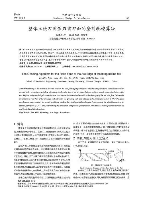
机械设计与制造Machinery Design & Manufacture147第6期2021年6月整体立铳刀圆弧刃前刀面的磨削轨迹算法张潇然,罗斌,陈思远,程雪峰(西南交通大学机械工程学院,四川成都610031)摘要:针对圆弧立铳刀磨削中周齿前刀面与端齿前刀面的过渡问题,提出磨削圆弧刃前刀面的砂轮轨迹算法,以此实现 周齿与端齿前刀面的光滑连接。
定义了一种切深磨削点轨迹曲线,可以同时约束圆弧前刀面的宽度和前角;定义了圆弧刃在平面中的瞬时前刀面,计算在瞬时前刀面中的砂轮磨削轨迹和姿态,再经过空间坐标变换,得出砂轮实际加工轨迹。
通过C++将算法编写为相应程序,进行仿真和实际加工验证,所得验证结果证明了该方法的正确性和可行性。
关键词:立铳刀;磨削加工;端齿圆弧刃;前刀面中图分类号:TH16;TH161 文献标识码:A 文章编号:1001-3997(2021)06-0147-03The Grinding Algorithm for the Rake Face of the Arc Edge of the Integral End MillZHANG Xiao-ran, LUO Bin, CHEN Si-yuan, CHENG Xue-feng(School of Mechanical Engineering , Southwest Jiaotong University, Sichuan Chengdu 610031, China)Abstract :A iming at the transition problem between the rake f ace of p eripheral f lank and the rake f ace of e nd tooth in the circulararc end mill, proposing a grinding algorithm f or the rake face of the arc edge that can achieve smooth connection between thetwo. Defines a depth-of-depth curve that can simultaneously constrain the width and rake angle of t he arc rake f ace. Defines theinstantaneous rake f ace of the arc edge and calculates the grinding path and attitude of t he grinding wheel in it. After the space coordinate transformation, the actual machining track of t he grinding wheel is obtained. Programming the algorithm into corre sponding p rogram by C++, and p erformming the simulation and p rocessing verification. The obtained results prove the correctnessand f easibility of t he algorithm.Key Words :End Mill ; Grinding ; Arc Edge ; Rake Face1引言圆弧头立铳刀是目前常见的高速切削刀具,具有制造成本低、材料切除率大等特点。
8形状优化
Update: Reparameterize or partition domains. Parameters: Update the morphing parameters. √ retain handles: 当在为新创建的或编辑的domain中的 √ partition domains:所有已创建的2D domain( shell单元或3D domain中的面)将被刨分。
2)改变handle间的距离
3)改变倒圆或孔的半径
4)绘制一新的曲面或线几何
HyperMorph操作来自domain的生成:create
Domain 的操作: Create: Create or update a domain. Organize: Move elements into a domain. Edit edges: Merge, split, or add handles to an
在HyperMorph中,通过Morphing操作来实 现网格的变形。Morphing过程包括将模型分成多 个domains(域),这些域的形状由handles(控 制柄)来控制。
Domains: 区域,模型的多个域 Handles:控制点,即Domains的对应控制点
Domain的分类:
全局 domain (globe domain) 局部 domain (local domain ) 1D
目 约 200Mpa
标: 质量最小化 束: 在接头部位的最大Von Mises 应力小于
设计变量: 接头的形状变量(使用HyperMorph 定义)
钢轨接头的形状优化
优化方案1
优化方案2
优化方案3=方案1+方案2
2010年11月CAESARII高级培训讲义- 工况编辑器 - 何耀良
z 载荷的形式应该进行独立的分析
z Magnification due to local variations
z 考虑了弯头、三通等管件的局部应力增大现象
z Code committee tradition
z 规范应力是规范委员会的传统惯例。
AECsoft
2010-11-6
CAESAR II 中所有的原始载荷
因此我们需要对工况进行组合编辑
AECsoft
2010-11-6
工况编辑器
推荐工况
AECsoft
原始载荷
组合工况
载荷循环次数 工况应力类型
2010-11-6
CAESAR II 工况设置
z 进行一次静态计算后,CAESAR II 保存最后 一次运算时的载荷工况设置。
z 注:CAESAR II 不会自动设置偶然工况,用 户需要根据实际情况灵活定义。
工况组合方法
z CAESARII中提供了多种工况组合方法,其中最常见 的有两类:
z Algebraic(代数合成): z 用于两个工况之间的减运算(求解EXP). z 分别求解相关工况的位移后再进行减运算得到位移差. z 通过最后得到的位移量来求解推力、弯矩、应力.
z Scalar(标量合成): z 用于两个工况之间的加运算(求解OCC). z 分别求解相关工况的应力后再进行叠加 z 不再单独计算各工况的位移
AECsoft
2010-11-6
组合工况
Used to add or subtract results from previously defined primitive load cases. 通过基础工况的加减获取特定的载荷要求。如在非线 性系统中重新计算风和地震载荷。 Necessary for proper EXP and OCC code stress definition. 考虑二次应力及偶然应力的工况组合。 Not used for restraint or equipment load definition, nor for displacement reporting. 有些特定的中间设计工况既不是计算推力也不是计算 位移,如弹簧设计工况
面向智能制造的不规则零件排样优化算法
Vol. 27 No. 6June2021第27卷第6期2 0 2 1年6月计算机集成制造系统Computer Integrated Manufacturing SystemsDOI : 10. 13196/j. cims. 2021. 06. 013面向智能制造的不规则零件排样优化算法高 勃X张红艳X朱明皓2+(1-北京交通大学计算机与信息技术学院'匕京100044;2.北京交通大学经济管理学院,北京100044&摘 要:以智能工厂应用场景为例,为提高广泛应用于智能制造领域的二维不规则件的排样性能,提出了基于启发式和蚁群的不规则件排样优化算法$首先提取不规则件的几何特征,对零件进行组合操作预处理,使两个或多个不规则零件组合为矩形件或近似矩形件并对其包络矩形,然后利用蚁群学习算法对预处理后的零件进行排样,确定零件排放的最佳位置,不断更新得到最优排样结果。
仿真实验结果表明,综合考虑板材利用率以及耗时情况,所提算法取得了较好的结果能总够满足实际生产的需求$关键词:二维板材;不规则零件;启发式算法;蚁群学习算法;优化排样中图分类号:TP391文献标识码:AOptimization algorithm of irregular parts layout for intelligent manufacturingGAO B o 1 , ZHANG Hongyan 1 , ZHUMinghao 2(1. School of Computer and Information Technology, Beijing Jiaotong University ,Beijing 100044, China ;2. School of Economics and Management , Beijing Jiaotong University , Beijing 100044, China)Abstract :To improve the performance of two-dimensional irregularly shaped part layout in the field of intelligent manufacturing and smart factories 'an optimization algorithmbased on heuristics and ant colony optimizations wasproposed.Thegeometricfeaturesofirregularlyshapedpartswereextractedtopreprocesscombinatorialoperationof theseparts 'which madetwoormorepartscombineintorectangularorapproximatelyrectangularparts.Thentheant colony learning algorithm was used to find an initial combination of parts.After irregularly shaped parts are nes- ted 'thebestpositionofeachpartwasdeterminedandoptimizediteratively.Theresultsofsimulationexperimentsshowed that the algorithm had achieved satisfactory results in terms of the utilization rate ofboards and time-com-plexity 'which madeareasonablesolutiontobeadoptedforactualproductions.Keywords :two-dimensional plate ; irregular parts ; heuristic algorithm ; ant colony learning algorithm ; optimized lay outo 引言二维零件排样是实际应用中最常见的排样问题,广泛应用在机械制造、轻工、服装和印刷业等行业中。
螺杆压缩机外文文献翻译、中英文翻译、外文翻译
螺杆压缩机外文文献翻译、中英文翻译、外文翻译英文原文Screw CompressorsN. Stosic I. Smith A. KovacevicScrew CompressorsMathematical Modellingand Performance CalculationWith 99 FiguresABCProf. Nikola StosicProf. Ian K. SmithDr. Ahmed KovacevicCity UniversitySchool of Engineering and Mathematical SciencesNorthampton SquareLondonEC1V 0HBU.K.e-mail:n.stosic@/doc/d6433edf534de518964bcf 84b9d528ea81c72f87.htmli.k.smith@/doc/d6433edf534de51896 4bcf84b9d528ea81c72f87.htmla.kovacevic@/doc/d6433edf534de51 8964bcf84b9d528ea81c72f87.htmlLibrary of Congress Control Number: 2004117305ISBN-10 3-540-24275-9 Springer Berlin Heidelberg New York ISBN-13 978-3-540-24275-8 Springer Berlin Heidelberg New YorkThis work is subject to copyright. All rights are reserved, whether the whole or part of the material is concerned, specifically the rights of translation, reprinting, reuse of illustrations, recitation, broadcasting, reproduction on microfilm or in any other way, and storage in data banks. Duplication of this publication or parts thereof is permitted only under the provisions of the German Copyright Law of September 9, 1965, in its current version, and permission for use must always be obtained from Springer. Violations are liable for prosecution under the GermanCopyright Law.Springer is a part of Springer Science+Business Media/doc/d6433edf534de518964bcf84b9d 528ea81c72f87.html_c Springer-Verlag Berlin Heidelberg 2005Printed in The NetherlandsThe use of general descriptive names, registered names, trademarks, etc. in this publication does not imply,even in the absence of a specific statement, that such names are exempt from the relevant protective laws and regulations and therefore free for general use.Typesetting: by the authors and TechBooks using a Springer LATEX macro packageCover design: medio, BerlinPrinted on acid-free paper SPIN: 11306856 62/3141/jl 5 4 3 2 1 0PrefaceAlthough the principles of operation of helical screw machines, as compressors or expanders, have been well known for more than 100 years, it is only during the past 30 years thatthese machines have become widely used. The main reasons for the long period before they were adopted were their relatively poor efficiency and the high cost of manufacturing their rotors. Two main developments led to a solution to these difficulties. The first of these was the introduction of the asymmetric rotor profile in 1973. This reduced the blowhole area, which was the main source of internal leakage by approximately 90%, and thereby raised the thermodynamic efficiency of these machines, to roughly the same level as that of traditional reciprocating compressors. The second was the introduction of precise thread milling machine tools at approximately the same time. This made it possible to manufacture items of complex shape, such as the rotors, both accurately and cheaply.From then on, as a result of their ever improving efficiencies, high reliability and compact form, screw compressors have taken an increasing share of the compressor market, especially in the fields of compressed air production, and refrigeration and air conditioning, and today, a substantial proportion of compressors manufactured for industry are of this type.Despite, the now wide usage of screw compressors and the publication of many scientific papers on their development, only a handful of textbooks have been published to date, which give a rigorous exposition of the principles of their operation and none of these are in English.The publication of this volume coincides with the tenth anniversary of the establishment of the Centre for Positive Displacement Compressor Technology at City University, London, where much, if not all, of the material it contains was developed. Its aim is to give an up to date summary of the state of the art. Its availability in a single volume should then help engineers inindustry to replace design procedures based on the simple assumptions of the compression of a fixed mass of ideal gas, by more up to date methods. These are based on computer models, which simulate real compression and expansion processes more reliably, by allowing for leakage, inlet and outlet flow and other losses, VI Preface and the assumption of real fluid properties in the working process. Also, methods are given for developing rotor profiles, based on the mathematical theory of gearing, rather than empirical curve fitting. In addition, some description is included of procedures for the three dimensional modelling of heat and fluid flow through these machines and how interaction between the rotors and the casing produces performance changes, which hitherto could not be calculated. It is shown that only a relatively small number of input parameters is required to describe both the geometry and performance of screw compressors. This makes it easy to control the design process so that modifications can be cross referenced through design software programs, thus saving both computer resources and design time, when compared with traditional design procedures.All the analytical procedures described, have been tried and proven on machines currently in industrial production and have led to improvements in performance and reductions in size and cost, which were hardly considered possible ten years ago. Moreover, in all cases where these were applied, the improved accuracy of the analytical models has led to close agreement between predicted and measured performance which greatly reduced development time and cost. Additionally, the better understanding of the principles of operation brought about by such studies has led to an extension of the areas of application of screw compressors and expanders.It is hoped that this work will stimulate further interest in an area, where, though much progress has been made, significant advances are still possible.London, Nikola StosicFebruary 2005 Ian SmithAhmed KovacevicNotationA Area of passage cross section, oil droplet total surfacea Speed of soundC Rotor centre distance, specific heat capacity, turbulence model constantsd Oil droplet Sauter mean diametere Internal energyf Body forceh Specific enthalpy h = h(θ), convective heat transfer coefficient betweenoil and gasi Unit vectorI Unit tensork Conductivity, kinetic energy of turbulence, time constant m Massm˙ Inlet or exit mass flow rate m˙ = m˙ (θ)p Rotor lead, pressure in the working chamber p = p(θ)P Production of kinetic energy of turbulenceq Source term˙Q Heat transfer rate between the fluid and the compressor surroundin gs˙Q= ˙Q(θ)r Rotor radiuss Distance between the pole and rotor contact points, control volume surfacet TimeT Torque, Temperatureu Displacement of solidU Internal energyW Work outputv Velocityw Fluid velocityV Local volume of the compressor working chamber V = V (θ)˙VVolume flowVIII Notationx Rotor coordinate, dryness fraction, spatial coordinatey Rotor coordinatez Axial coordinateGreek Lettersα Temperature dilatation coefficientΓ Diffusion coefficientε Dissipation of kinetic energy of turbulenceηi Adiabatic efficiencyηt Isothermal efficiencyηv Volumetric efficiencySpecific variableφ Variableλ Lame coefficientμ Viscosityρ Densityσ Prand tl numberθ Rotor angle of rotationζ Compound, local and point resistance coefficientω Angular speed of rotationPrefixesd differentialΔ IncrementSubscriptseff Effectiveg Gasin Inflowf Saturated liquidg Saturated vapourind Indicatorl Leakageoil Oilout Outflowp Previous step in iterative calculations SolidT Turbulentw pitch circle1 main rotor, upstream condition2 gate rotor, downstream conditionContents1Introduction. . . . . . . . . . . . . . . . . . . . . . . . . . . . . . . . ………………………. . . . . . . . . . . . . . . 1 1.1 Basic Concepts . . . . . . . . . . . . . . . . . . . . . . . . . . . . . . . . . . . . . . . . . . . . . . . . . . . .. .. . . . . . . . . 4 1.2 Types of Screw Compressors . . . . . . . . . . . . . . . . . . . . . . . . . . . . . . . . . . . .. . . . . ….. . . . . . . .7 1.2.1 The Oil Injected Machine . . . . . . . . . . . . . . . . . . . . . . . . . . . . . . . . . . . . . . . . . . . . . …... . .71.2.2 The Oil Free Machine . . . . . . . . . . . . . . . . . . . . . . . . . . . . . . . . . . . . . . .. . . . . . . . . . . ….... .7 1.3 Screw Machine Design . . . . . . . . . . . . . . . . . . . . . . . . . . . . . . . . . . . . . . .. . . . . . . . . . . . . . . .8 1.4 Screw Compressor Practice . . . . . . . . . . . . . . . . . . . . . . . . . . . . . . . . . . .. . . . . . . . . . . . . . . . .101.5RecentDevelopments . . . . . . . . . . . . . . . . . . . . . . . . . . . . . . . . . . . . . . . . . . . . . . . . . . . . . . . . . 12 1.5.1RotorProfiles . . . . . . . . . . . . . . . . . . . . . . . . . . . . . . . . . . . . . . . . . . . . . . . . . . . . . . . . .. . . . . 13 1.5.2CompressorDesign . . . . . . . . . . . . . . . . . . . . . . . . . . . . . . . . . . . . . . . . . . . . . . . . . . . . . . . 17 2ScrewCompressorGeometry. . . . . . . . . . . . . . . . . . . . . . . . . . . . . . . . . . . . . . . . . . . . . . . . . . 192.1 The Envelope Method as a Basis for the Profiling of Screw CompressorRotors . . . . . . . . . . . . . . . . . . . . . . . . . . . . . . . . . . . ………………………….. . . . . ….. . . . . . . . 19 2.2 Screw Compressor Rotor Profile s . . . . . . . . . . . . . . . . . . . . …. . . . . . . . . . . . . . . . . . . ….. . . 20 2.3 Rotor ProfileCalculation . . . . . . . . . . . . . . . . . . . . . . . . . . . …………………………. . . . . .23 2.4 Review of Most Popular Rotor Profiles . . . . . . . . . . . . . . . ………………………….. . . . . . 23 2.4.1 Demonstrator Rotor Profile (“N” Rotor Generated) . . ………………………………….. . 24 2.4.2 SKBK Profile . . . . . . . . . . . . . . . . . . . . . . . . . . . ……………………………... . . . . . . . . .26 2.4.3 Fu Sheng Profile . . . . . . . . . . . . . . . . . . . . . . . . . ………………………………. . . . . . . . .27 2.4.4 “Hyper”Profile . . . . . . . . . . . . . . . . . . . . . . . . . . . . . . . . ………………………………. . .27 2.4.5 “Sigma” Profile . . . . . . . . . . . . . . . . . . . . . . .. . . . . . ………………………………. . . . . .28 2.4.6 “Cyclon” Profile . . . . . . . . . . . . . . . . . . . . . . . . . . . . ………………………………. . . . . .28 2.4.7 Symmetric Prof ile . . . . . . . . . . . . . . . . . . . . . . . . . . . ……………………………… . . . . .29 2.4.8 SRM “A” Profile . . . . . . . . . . . . . . . . . . . . . . . . . . ……………………………… . . . . . . .30 2.4.9 SRM “D” Profile . . . . . . . . . . . . . . . . . . . . . . . . . . . ……………………………… . . . . . .31 2.4.10 SRM “G” Profile . . . . . . . . . . . . . . . .. . . . . . . . …………………………….. . . . . . . . . .32 2.4.11 City “N” Rack Generated Rotor Profile . . . . . . . . . . . ………………………………… . . 32 2.4.12 Characteristics of “N” Profile . . . . . . . . . . . . . . . . . . . ………………………………. . . . 34 2.4.13 Blower Rot or Profile . . . . . . . . . . . . . . . . . . . . …………………………….. . . . . . . . . . . 39 X Contents2.5 Identification of Rotor Positionin Compressor Bearings . . . . . . . . . . . . . . . . . . . . . . . . . . …………………………….. . . . . . . .40 2.6 Tools for Rotor Manufacture . . . . . . . . . . . . . . . . . . . . . . …………………………. . . . . . . .45 2.6.1 Hobbing Tools . . . . . . . . . . . . . . . . . . . . . . . . . . ………….…..………………. . . . . . . . . .45 2.6.2 Milling and Grinding Tools . . . . . . . . . . . . . . . . . . . ……………………………….... . . . . 482.6.3 Quantification of ManufacturingImperfections . . . . . ……………………………….... . . 483 Calculation of Screw Compressor Performance . . . . . . . . . . ………………………………. . . 49 3.1 One Dimensional Mathematical Model . . . . . . . . . . . . . . …………………………... . . . . . .49 3.1.1 Conservation Equationsfor Control Volume and Auxiliary Relationships . . . . ............................................... . . 50 3.1.2 Suction and Discharge Ports . . . . . . . . . . . . . . . . . . . ....................................... . . . . 53 3.1.3 Gas Leakages . . . . . . . . . . . . . . . . . . . . . . . . . . .................................... . . . . . . . . . .54 3.1.4 Oil or Liquid Injection . . . . . . . . . . . ...................................... . . . . . . . . . . . . . . . . . 55 3.1.5 Computation of Fluid Properties . . . . . . . . ........................................ . . . . . . . . . . . 57 3.1.6 Solution Procedure for Compressor Thermodynamics . (58)3.2 Compressor Integral Parameters . . . . . . . . . . . . . . . . . . . ………………………….. . . . . . . . 59 3.3 Pressure Forces Actingon Screw Compressor Rotors . . . . . . . . . . . . . . . . . . . . . . ................................... . . . . . . . 61 3.3.1 Calculation of Pressure Radial Forces and Torque . . . . .. (61)3.3.2 Rotor Bending Deflections . . . . . . . . . . . . . . . . . . . . . ……………………………….. . . . 64 3.4 Optimisation of the Screw Compressor Rotor Profile,Compressor Design and Operating Parameters . . . . . . . . . . ……………………………….. . . . 65 3.4.1 OptimisationRationale . . . . . . . . . . . . . . . . . . . . . . . . ……………………………….. . . . 65 3.4.2 Minimisation Method Usedin Screw CompressorOptimisation . . . . . . . . . . . ……………………………………… . . . . . . 67 3.5 Three Dimensional CFD and Structure Analysisof a Screw Compressor . . . . . . . . . . . . . . . . . . . . . . . . . …………………………….. . . . . . . . .71 4 Principles of Screw Compressor Design. . . . . . . . . . . …………………………… . . . . . . . . 77 4.1 Clearance Management. . . . . . . . . . . . . . . . . . . . . . . . ………….….………… . . . . . . . . . .78 4.1.1 Load Sustainability . . . . . . . . . . . . . . . . . . . . . . . . . . . . ………….………………….. . . .79 4.1.2 Compressor Size and Scale . . . . . . . . . . . . . . ………………………………. . . . . . . . . . . 80 4.1.3 RotorConfiguration . . . . . . . . . . . . . . . . . . . . . . . ……………………………... . . . . . . .82 4.2 Calculation Example:5-6-128mm Oil-Flooded Air Compressor . . . . . . . . . . . . . . . ……………………………... . . . 824.2.1 Experimental Verification of the Model . . . . . . . . . . . ………………………………. . . . 845 Examples of Modern Screw Compressor Designs . . . . . . . ……………………………… . . . 89 5.1 Design of an Oil-Free Screw CompressorBased on 3-5 “N” Rotors . . . . . . . . . . . . . . . . . . . . . . . . . . ……………………………. . . . . . . 90 5.2 The Design of Familyof Oil-Flooded Screw Compressors Basedon 4-5 “N” Rotors . . . . . . . . . . . . . . . . . . . . . . . . . . . . . . . …………………………… . . . . . . .93 Contents XI.5.3 Design of Replacement Rotorsfor Oil-FloodedCompressors . . . . . . . . . . . . . . . . . . . . . . . . . . . ................................. . .96 5.4 Design of Refrigeration Compressors . . . . . . . . . . . . . . . .............................. . . . . . . 100 5.4.1 Optimisation of Screw Compressors for Refrigeration . . . (102)5.4.2 Use of New Rotor Profiles . . . . . . . . . . . . . . . . . . . . . . . . . . (103)5.4.3 Rotor Retrofits . . . . . . . . . . . . . . . . . . . . . . . . . . . . . . . . . ……………………………. . . 103 5.4.4 Motor Cooling Through the Superfeed Port in Semihermetic Compressors . . . . . . . . . . . . . . . . . . . …………………………………… . . . 103 5.4.5 Multirotor Screw Compressors . . . . . . . . . . . . . . . . . …………………………….... . . . . 104 5.5 Multifunctional Screw Machines . . . . . . . . . . . . . . . . . . ……………………….. . . . . . . . . 108 5.5.1 Simultaneous Compression and Expansionon One Pair of Rotors . . . . . . . . . . . . . . . . . . . . . . . . . . ............................................ . 108 5.5.2 Design Characteristics of Multifunctional Screw Rotors .. (109)5.5.3 Balancing Forces on Compressor-Expander Rotors . …………………..……………. . . 1105.5.4 Examples of Multifunctional Screw Machines . . . . . . . . (111)6Conclusions. . . . . . . . . . . . . . . . . . . . . . . . . . . . . . . . . . . . . . …………………… . . . . . . . . . 117A Envelope Method of Gearin g . . . . . . . . . . . . . . . . . . . . . . . . ………………………… . . . . . 119B Reynolds TransportTheorem. . . . . . . . . . . . . . . . . . . . . . . …………………………. . . . . . . 123C Estimation of Working Fluid Propertie s . . . . . . . . . . . . . . . …………………………….. . . . 127 Re ferences. . . . . . . . . . . . . . . . . . . . . . . . . . . . . . . . . . . . . . . . . . ………………… . . . . . . . . . . 133中文译文螺杆压缩机N.斯托西奇史密斯先生A科瓦切维奇螺杆压缩机计算的数学模型和性能尼古拉教授斯托西奇教授伊恩史密斯博士艾哈迈德科瓦切维奇工程科学和数学北安普敦广场伦敦城市大学英国电子邮件:n.stosic@/doc/d6433edf534de518964bcf 84b9d528ea81c72f87.htmli.k.smith@/doc/d6433edf534de51896 4bcf84b9d528ea81c72f87.htmla.kovacevic@/doc/d6433edf534de51 8964bcf84b9d528ea81c72f87.html国会图书馆控制号:2004117305isbn-10 3-540-24275-9 纽约施普林格柏林海德堡isbn-13 978-3-540-24275-8 纽约施普林格柏林海德堡这项工作是受版权保护,我们保留所有权利。