Exponential Distributions in a Mechanical Model for Earthquakes
The influence of biological fluids on crack spacing distribution in Si-DLC films on steel substrates
coatings in improving the mechanical, thermal and chemical performance of various substrates has been further highlighted in a recent (2002) paper by Ganne et al. [1]. Silicon doping improves the adhesion of DLC to some metallic substrates [2,3] and silicon modified DLC is currently being investigated as a protective coating for stainless steel for biocompatible and haemocompatible functions in body implants [4]. The development of such coatings will lead to the usage of stainless steel in biomedical implants where its superior mechanical performance can be used to considerable advantage [5–7]. However, if coatings and films like DLC and
A.A. Ogwu a,∗ 1, T. Coyle b, T.I.T. Okpalugo a, P. Kearney a, P.D. Maguire a, J.A.D. MEC, School of Electrical and Mechanical Engineering, University of Ulster, Shore Road, Co. Antrim BT37 0QB, Northern Ireland, UK Department of Materials Science and Engineering, University of Toronto, 184 College St, Toronto, ON, Canada M5S 3E4
论文投稿注意事项-爱思维尔专家总结
Title, Author and Affiliation_ 文题:简洁、清楚、充分地表达文章内容,避免无意义的词_ 作者:指明通讯作者。
确认所有作者都对文章作出了贡献,并同意发表文章_ 作者排序:_ 第一作者是对数据收集和分析以及论文撰写负有主要责任的人_ 最后一位作者,通常是有学术地位的研究人员,对整个研究负有责任;_ 位列中间者的顺序则视其对研究所做出的贡献而定_ 通讯作者的排名是不重要的,但一旦选择成为了通讯作者,就要对这篇文章在审阅过程中的所有通信交流质询做出负责的回应。
_ 作者机构:所有作者的机构信息Abstract_ 简要介绍文章内容和研究目的_ 关键结论的简要描述_ 不要涉及太多的实验细节_ 不超过250字_ 摘要是论文最先被阅读的部分_ 摘要,题名含混不清/不科学论文的缩微模型:做了什么,得到了哪些重要结果Abstract.I&M = 做了什么I---We tackle the general linear instantaneous model (possibly underdetermined and noisy) where we model the source prior with a Student t distribution. The conjugate-exponential characterisation ofthe t distribution as an infinite mixture of scaled Gaussians enables usto do efficient inference. M---We study two well-known inference methods, Gibbs sampler and variational Bayes for Bayesian source separation.We derive both techniques as local message passing algorithms to highlight their algorithmic similarities and to contrast their different convergence characteristics and computational requirements.R&D=主要发现是什么R---Our simulation results suggest that typical posterior distributions in source separation have multiple local maxima. Therefore we proposea hybrid approach where we explore the state space with a Gibbssampler and then switch to a deterministic algorithm. D---This approach seems to be able to combine the speed of the variational approachwith the robustness of the Gibbs sampler.Introduction简短,重点突出_ 研究的重要性_ What is the problem?_ Are there any existing solutions?_ Which is the best?_ What is its main limitation?_ What do you hope to achieve?注意:论述问题、研究目的及研究方法,但不要说明结论、展开讨论或进行总结(应包含在Abstract中)_ 引用对应领域重要的及最新的著作(30篇以内)_ 评审人员评审角度_ 有效性、论述清楚、内容组织_ 相关重要的文献是否包含Methods_ 基本原则:提供足够的信息,以便读者能够重复试验或推倒的过程。
多元混合指数分布参数的优化估计的开题报告

多元混合指数分布参数的优化估计的开题报告一、研究背景指数分布是重要的概率分布之一,广泛应用于各个领域。
然而,在实际应用中,往往需要对多元混合指数分布进行估计。
多元混合指数分布是由多个指数分布叠加得到的概率分布模型,其在实际应用中能更好地描述数据的特征。
因此,如何对多元混合指数分布的参数进行优化估计,成为当前研究的重要问题。
二、研究问题本文旨在研究如何对多元混合指数分布的参数进行优化估计。
具体来说,研究问题包括:1. 如何选择合适的优化算法对多元混合指数分布参数进行估计?2. 如何确定多元混合指数分布的“混合比例”参数?3. 如何对估计结果进行可靠性检验?三、研究内容本文将以多元混合指数分布参数的优化估计为主要研究内容,具体包括以下几个方面:1. 对多元混合指数分布的相关知识进行总结和归纳,包括理论基础、分布特征、分布参数等方面。
2. 针对多元混合指数分布中存在的问题,提出相应的优化估计策略,建立合适的估计模型。
3. 分析不同的优化算法对多元混合指数分布参数的影响,从而选择合适的优化算法进行参数估计。
4. 结合实际应用中数据的特点,确定多元混合指数分布的“混合比例”参数。
5. 对估计结果进行可靠性检验,评估模型的拟合效果和预测精度。
四、研究意义通过对多元混合指数分布参数的优化估计,可以更准确地描述数据的特征和规律,提高数据分析和预测的精度和准确性,在实际应用中具有重要的应用价值。
此外,本文还可以丰富多元概率分布的理论研究,为其它相关领域的研究提供参考。
五、研究方法本文将采用文献研究、理论分析和实证研究相结合的方法,具体如下:1. 文献研究:通过查阅相关文献,总结多元混合指数分布的理论基础、分布特征、分布参数以及相关优化估计方法等。
2. 理论分析:在文献研究的基础上,借助数学方法、统计学方法等对多元混合指数分布参数的优化估计进行理论分析和求解。
3. 实证研究:通过使用实际数据,对所提出的多元混合指数分布参数的优化估计方法进行实证研究,评估模型的拟合效果和预测精度,并与其它方法进行对比。
Selected_Texts_in_Mathematics1

4
Let A= Then AB = 6 13 −3 −4 and BA = 2 3 −5 0 2 1 −1 0 and B = 3 4 0 5
Thus, AB = BA. Properties of matrix addition and multiplication 1. A + B = B + A 2. (A + B) + C = A + (B + C) 3. A − A = 0 and A + 0 = A 4. (α + β )A = αA + β A 5. α(A + B) = αA + αB 6. (αβ )A = α(β A) 7. (AB)C = A(BC) 8. A(B + C) = AB + AC 9. IA = AI = A and 0A = A0 = 0 10. In general, AB = BA, even when both products are defined. Trace of a square matrix If A is a square matrix, the trace of A, denoted tr(A), is the sum of the elements on
1.1
Definitions
Matrix A matrix is a rectangular array of numbers. A matrix with dimension m × n has m rows and n columns. As an example, consider the following matrix A= 2 −1 7 −4 5 0 2
1
1
Discriminating large extra dimensions at the ILC with polarized beams
a r X i v :h e p -p h /0604047v 1 5 A p r 20062005ALCPG &ILC Workshops -Snowmass,U.S.A.Discriminating Large Extra Dimensions at the ILC with Polarized BeamsA.A.Pankov,A.V .TsytrinovPavel Sukhoi Technical University,Gomel 246746,BelarusN.PaverUniversity of Trieste and INFN,34100Trieste,ItalyNon-standard scenarios described by effective interactions can manifest themselves indirectly,via corrections to the Standard Model cross sections.It should be desirable to identify at a given confidence level the source of such deviations among the different possible explanations.We here discuss the identification reach on gravity in extra dimensions from the four-fermion compositeness-inspired contact interactions and viceversa ,using as basic observable the differential cross section of e +e −→¯ff at the ILC,and emphasize the rˆo le of beams polarization in enhancing the identification sensitivity.1.INTRODUCTION New-physics scenarios (NP)based on very heavy virtual quanta exchanges can be described,below the direct production threshold,by effective,contact-interactions that can can have only indirect signatures by contributing corrective terms to the Standard Model (SM)amplitudes,suppressed by some power of the ratio between the collider c.m.energy and the above mentioned characteristic high mass scales.These corrections will reveal themselves via deviations of the measured observables from the SM predictions or,in few specific cases,by the observation of processes forbidden by the SM.In principle,different kinds of NP interactions may produce similar deviations and,consequently,it would be desirable to assess,for each non-standard model,not only the “discovery reach”,represented by the maximal value of the relevant mass scale below which a deviation can be observed at a given C.L.within the experimental accuracy but,also,the “identification reach”,defined as the upper limit of the mass range of values for which the model can be discriminated from the other potentially competing scenarios.We will focus on the discrimination reach on the ADD models of gravity in large,compactified,extra spatial dimensions [1],with respect to the four-fermion contact interactions inspired by compositeness [2],and viceversa ,looking at the differential cross sections ofe ++e −→¯f +f,(1)with f =l,q (l =µ,τ;q =c,b ),at the ILC with longitudinally polarized beams [3,4].In Ref.[5],the identification reach on individual contact-interactions was studied by applying a Monte Carlo technique to lepton-pair production with unpolarized beams.An approach based on the polarized differential distributions for lepton pair production processes was proposed in Ref.[6].We here discuss the benefits of longitudinal beams polarization in improving the identification reaches and consider also quark-pair production channels.2.DIFFERENTIAL CROSS SECTIONS AND DEVIATIONS FROM THE SMNeglecting all fermion masses with respect to the c.m.energy√dz =1dz +dσLRdz +dσRLwhere z=cosθis the angle between the incoming and outgoing fermions in the c.m.frame and(α,β=L,R):dσαβσpt|Mαβ|2(1±z)2.(3)8P1and P2the degrees of longitudinal polarization of the electron and positron beams,respectively,and the‘±’signs apply to the cases LL,RR and LR,RL,respectively.According to sec.1,the reduced helicity amplitudes appearing in Eq.(3)can be expanded into the SM part represented byγand Z exchanges,plus corrections depending on the considered NP model:Mαβ=M SMαβ+∆αβ(NP).(4) The examples explicitly considered here are the following ones:a)The ADD large extra dimensions scenario[1],where only gravity can propagate in extra dimensions,and correspondingly a tower of graviton KK states occurs in the four-dimensional space[8,9].In the parameterization of Ref.[10],the(z-dependent)deviations can be expressed as[11]:∆LL(ADD)=∆RR(ADD)=f G(1−2z),∆LR(ADD)=∆RL(ADD)=−f G(1+2z),(5) where f G=λs2/(4παe.m.Λ4H),λ=±1,ΛH being a phenomenological cut-offon the integration on the KK spectrum.b)Gravity in TeV−1–scale extra dimensions,where also the SM gauge bosons can propagate there,parameterized by the“compactification scale”M C[12,13]:∆αβ(TeV)=− Q e Q f+g eαg fβ π2/(3M2C).(6) c)The four-fermion contact-interaction scenario(CI)[2]where,withΛαβthe“compositeness”mass scales(ηαβ=±1):∆αβ(CI)=ηαβs/(αe.m.Λ2αβ).(7) In cases b)and c)the deviations are z-independent,whereas in the case a)they introduce extra z-dependence in the angular distributions.The consequence is that the ADD contribution to the integrated cross sections is tiny, because the interference with the SM amplitudes vanishes in these observables.Current experimental lower bounds on the mass scales M H and M C are reviewed,e.g.,in Ref.[14](M H>1.1−1.3TeV,M C>6.8TeV),while those on Λs,of the order of10TeV,are detailed in Ref.[15].3.DERIVATION OF THE IDENTIFICATION REACHESLet us assume one of the models,for example the ADD model(5),to be the“true”one,i.e.,to be consistent with data for some value ofΛH.To estimate the level at which it may be discriminated from other,in principle competing NP scenarios(“tested”models),for any values of the relevant mass parameters,say example one of the four-fermion CI models(7),we introduce relative deviations of the differential cross section(denoted by O)from the ADD predictions due to the CI in each angular bin,and a correspondingχ2function:2.(8)∆(O)=O(CI)−O(ADD)δO binHere,δO s represent the expected relative uncertainties,which combine statistical and systematic ones,the former one being related to the ADD model prediction.Consequently,theχ2of Eq.(8)is a function ofλ/Λ4H and the considered η/Λ2,and we can determine the“confusion”region in this parameter plane where also the corresponding CI model may be considered as consistent with the ADD predictions at the chosen confidence level,so that an unambiguous identification of ADD cannot be made.We chooseχ2<3.84for95%C.L..ALCPG0112√For the numerical analysis,we consider an ILC withFigure 2:95%CL identification reach on the cutoffscale M C in the TeV model (left panel)and ΛVV in the VV model (right panel)as a function of the integrated luminosity obtained from the fermion pair production processes with unpolarized and both polarized beams at ILC(0.5TeV).References[1]N.Arkani-Hamed,S.Dimopoulos and G.R.Dvali,Phys.Lett.B 429,263(1998);N.Arkani-Hamed,S.Dimopoulos and G.R.Dvali,Phys.Rev.D 59,086004(1999);I.Antoniadis,N.Arkani-Hamed,S.Dimopoulos and G.R.Dvali,Phys.Lett.B 436,257(1998).[2]E.Eichten,ne and M.E.Peskin,Phys.Rev.Lett.50,811(1983);R.R¨u ckl,Phys.Lett.B 129,363(1983).[3]J.A.Aguilar-Saavedra et al.[ECFA/DESY LC Physics Working Group Collaboration],“TESLA TechnicalDesign Report Part III:Physics at an e +e −Linear Collider,”DESY-01-011,arXiv:hep-ph/0106315;T.Abe et al.[American Linear Collider Working Group Collaboration],“Linear collider physics resource book for Snowmass 2001.1:Introduction,”in Proc.of the APS/DPF/DPB Summer Study on the Future of Particle Physics (Snowmass 2001)SLAC-R-570,arXiv:hep-ex/0106055.[4]G.Moortgat-Pick et al.,arXiv:hep-ph/0507011.[5]G.Pasztor and M.Perelstein,in Proc.of the APS/DPF/DPB Summer Study on the Future of Particle Physics(Snowmass 2001)ed.N.Graf,arXiv:hep-ph/0111471.[6]A.A.Pankov,N.Paver and A.V.Tsytrinov,[arXiv:hep-ph/0512131].[7]B.Schrempp,F.Schrempp,N.Wermes and D.Zeppenfeld,Nucl.Phys.B 296,1(1988).[8]T.Han,J.D.Lykken and R.J.Zhang,Phys.Rev.D 59,105006(1999)[arXiv:hep-ph/9811350].[9]G.F.Giudice,R.Rattazzi and J.D.Wells,Nucl.Phys.B 544,3(1999)[arXiv:hep-ph/9811291].[10]J.L.Hewett,Phys.Rev.Lett.82,4765(1999)[arXiv:hep-ph/9811356].[11]S.Cullen,M.Perelstein and M.E.Peskin,Phys.Rev.D 62,055012(2000)[arXiv:hep-ph/0001166].[12]K.M.Cheung and ndsberg,Phys.Rev.D 65,076003(2002)[arXiv:hep-ph/0110346].[13]T.G.Rizzo and J.D.Wells,Phys.Rev.D 61,016007(2000)[arXiv:hep-ph/9906234].[14]For a review see,e.g.,K.Cheung,arXiv:hep-ph/0409028.[15]S.Eidelman et al.[Particle Data Group],Phys.Lett.B 502,1(2004).ALCPG0112。
(完整word版)英文版概率论与数理统计重点单词

概率论与数理统计中的英文单词和短语概率论与数理统计Probability Theory and Mathematical Statistics第一章概率论的基本观点Chapter 1Introduction of Probability Theory不确立性indeterminacy必定现象certain phenomenon随机现象random phenomenon试验experiment结果outcome频次数frequency number样本空间sample space出现次数frequency of occurrencen 维样本空间n-dimensional sample space样本空间的点point in sample space随机事件random event / random occurrence基本领件elementary event必定事件certain event不行能事件impossible event等可能事件equally likely event事件运算律operational rules of events事件的包括implication of events并事件union events交事件intersection events互不相容事件、mutually exclusive exvents/互斥事件/incompatible events互逆的mutually inverse加法定理addition theorem古典概率classical probability古典概率模型classical probabilistic model几何概率geometric probability 乘法定理product theorem概率乘法multiplication of probabilities条件概率conditional probability全概率公式、全formula of total probability概率定理贝叶斯公式、逆Bayes formula概率公式后验概率posterior probability先验概率prior probability独立事件independent event独立随机事件independent random event独立实验independent experiment两两独立pairwise independent两两独立事件pairwise independent events第二章随机变量及其散布Chapter2Random Variables and Distributions随机变量random variables失散随机变量discrete random variables概率散布律law of probability distribution一维概率散布one-dimension probability distribution 概率散布probability distribution两点散布two-point distribution伯努利散布Bernoulli distribution二项散布 / 伯努Binomial distribution利散布超几何散布hypergeometric distribution三项散布trinomial distribution多项散布polynomial distribution泊松散布Poisson distribution泊松参数Poisson theorem散布函数distribution function概率散布函数probability density function连续随机变量continuous random variable概率密度probability density概率密度函数probability density function概率曲线probability curve平均散布uniform distribution指数散布exponential distribution指数散布密度函exponential distribution density 数function正态散布、高斯normal distribution散布标准正态散布standard normal distribution正态概率密度函normal probability density function数正态概率曲线normal probability curve标准正态曲线standard normal curve柯西散布Cauchy distribution散布密度density of distribution第三章多维随机变量及其散布Chapter 3 Multivariate Random Variables and Distributions二维随机变量two-dimensional random variable结合散布函数joint distribution function二维失散型随机two-dimensional discrete random 变量variable二维连续型随机two-dimensional continuous random 变量variable结合概率密度joint probability variablen 维随机变量n-dimensional random variablen 维散布函数n-dimensional distribution functionn 维概率散布n-dimensional probability distribution边沿散布marginal distribution边沿散布函数marginal distribution function边沿散布律law of marginal distribution边沿概率密度marginal probability density二维正态散布two-dimensional normal distribution二维正态概率密two-dimensional normal probability 度density 二维正态概率曲two-dimensional normal probability 线curve条件散布conditional distribution条件散布律law of conditional distribution条件概率散布conditional probability distribution条件概率密度conditional probability density边沿密度marginal density独立随机变量independent random variables第四章随机变量的数字特点Chapter 4 Numerical Characteristics fo Random Variables数学希望、均值mathematical expectation希望值expectation value方差variance标准差standard deviation随机变量的方差variance of random variables均方差mean square deviation有关关系dependence relation有关系数correlation coefficient协方差covariance协方差矩阵covariance matrix切比雪夫不等式Chebyshev inequality第五章大数定律及中心极限制理Chapter 5 Law of Large Numbers and Central Limit Theorem大数定律law of great numbers切比雪夫定理的special form of Chebyshev theorem特别形式依概率收敛convergence in probability伯努利大数定律Bernoulli law of large numbers同散布same distribution列维 - 林德伯格independent Levy-Lindberg theorem定理、独立同分布中心极限制理辛钦大数定律Khinchine law of large numbers利亚普诺夫定理Liapunov theorem棣莫弗 - 拉普拉De Moivre-Laplace theorem斯定理第六章样本及抽样分布Chapter 6 Samples and Sampling Distributions统计量statistic整体population个体individual样本sample容量capacity统计剖析statistical analysis统计散布statistical distribution统计整体statistical ensemble随机抽样stochastic sampling / random sampling 随机样本random sample简单随机抽样simple random sampling简单随机样本simple random sample经验散布函数empirical distribution function样本均值sample average / sample mean样本方差sample variance样本标准差sample standard deviation标准偏差standard error样本 k 阶矩sample moment of order k样本中心矩sample central moment样本值sample value样本大小、样本sample size容量样本统计量sampling statistics 随机抽样散布random sampling distribution抽样散布、样本sampling distribution散布自由度degree of freedomZ 散布Z-distributionU 散布U-distribution第七章参数预计Chapter 7Parameter Estimations统计推测statistical inference参数预计parameter estimation散布参数parameter of distribution参数统计推测parametric statistical inference点预计point estimate / point estimation整体中心距population central moment整体有关系数population correlation coefficient整体散布population covariance整体协方差population covariance点预计量point estimator预计量estimator无偏预计unbiased estimate/ unbiasedestimation预计量的有效性efficiency of estimator矩法预计moment estimation整体均值population mean整体矩population moment整体 k 阶矩population moment of order k整体参数population parameter极大似然预计maximum likelihood estimation极大似然预计量maximum likelihood estimator极大似然法maximum likelihood method /maximum-likelihood method似然方程likelihood equation似然函数likelihood function区间预计interval estimation置信区间confidence interval置信水平confidence level置信系数confidence coefficient单侧置信区间one-sided confidence interval置信上限置信下限U 预计正态整体整体方差的预计confidence upper limit confidence lower limitU-estimatornormal populationestimation of population variance置信度方差比degree of confidence variance ratio第八章假定查验Chapter 8Hypothesis Testings参数假定假定查验两类错误统计假定统计假定查验查验统计量明显性查验统计明显性parametric hypothesis hypothesis testingtwo types of errors statistical hypothesis statistical hypothesis testing test statisticstest of significance statistical significance单边查验、单侧one-sided test查验单侧假定、单边one-sided hypothesis 假定两侧假定两侧查验明显水平拒绝域 / 否认区two-sided hypothesis two-sided testing significant level rejection region域接受地区acceptance regionU 查验F 查验方差齐性的查验拟合优度查验U-testF-testhomogeneity test for variances test of goodness of fit。
Process
180
6. TIME SERIES AND STOCHASTIC PROCESSES
R( s, t) = Cov[X ( s), X .1. Stationary time series
Stationarity is a basic assumption in classical time series analysis. It means, in effect, that the main statistical properties of the series remain unchanged over time. More precisely, a process {X (t)} is said to be completely stationary or strict sense stationary (abbreviated as S S S ) if the process X (t) and X (t + c) have the same statistics for any c. That is for any set of time points t1 , t2 , · · · , tn and any integer c, the joint probability distribution of [X (t1 ), X (t2 ), · · · , X (tn )] is identical with that of [X (t1 + c), X (t2 + c), · · · , X (tn + c)]. Less stringently, a process {X (t)} is said to be covariance stationary (second order stationary) or wide sense stationary (abbreviated as WS S ) if the mean and variance of X (t) remain constant over time and the autocovariance between any two values depends only on the time difference and not on their individual locations. That is, (i) E [X (t)] = µ, independent of t (ii) Var[X (t)] = σ2 x , independent of t (iii) Cov[X (t), X (t + s)] = R( s). It may be noted that S S S implies WS S , but the converse is not true always. (6.1.2)
概率论与数理统计(英文) 第四章
(4.1.2)
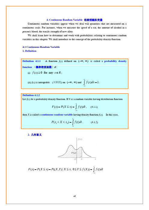
2. 几何意义
F ( x) = P( X ≤ x) = P(( X , Y ) | X ≤ x, 0 ≤ Y ≤ f ( X )) =
∞
∫
x
f (t )dt
46
P( x1 < X < x2 ) =
x2
∫ f (t )dt
x1
3. Note In most applications, f(x) is either continuous or piecewise continuous having at most finitely many discontinuities. Note 1 For a random variable X, we have a distribution function. If X is discrete, it has a probability distribution. If X is continuous, it has a probability density function. Note 2 Let X be a continuous random variable, then for any real number x,
x /(b a ) , regardless of the exact location of the interval.
To find the mean and variance of the uniform distribution
1
π
.
(Cauchy distribution 柯西分布 柯西分布) □ Example 4.1.3 Calculating probabilities from the probability density function If a random variable has the probability density
- 1、下载文档前请自行甄别文档内容的完整性,平台不提供额外的编辑、内容补充、找答案等附加服务。
- 2、"仅部分预览"的文档,不可在线预览部分如存在完整性等问题,可反馈申请退款(可完整预览的文档不适用该条件!)。
- 3、如文档侵犯您的权益,请联系客服反馈,我们会尽快为您处理(人工客服工作时间:9:00-18:30)。
Typeset using REVTEX 1
I. INTRODUCTION
Systems that present stick-slip dynamics and scaling invariance have attracted considerable attention recently [1,2]. This was triggered, in part, by a seminal paper of Bak, Tang and Wiesenfeld, which showed that a class of systems presenting avalanches ou earthquakelike dynamics can naturally attain a critical state characterized by power-law distributions [1]. They denoted this phenomenon Self-Organized Criticality. Recently, two experimental studies in a continuous elastic system have been performed to model the stick-slip dynamics observed in earthquake-like phenomena. In one of them [3], a glass rod is pulled on top of a latex membrane. In this system the slipping events appear as detachment waves and a wide distribution of event sizes was observed. However, robust scaling behavior was not seen. In the other system [4], the elastic medium consists of a transparent gel sheared between two coaxial circular cylinders. The inner cylinder is rotated at very low angular speed. Thus, this system closely resembles the physics of a spring-block model [5] with periodic boundary conditions. Due to the friction between the gel and the cylinders, stick-slip behavior is seen in the form of detachment waves. Rubio and Galeano were able to identify four regimes in this system, by varying the gel’s rigidity, the rotor angular speed and the friction properties of the gel with the inner cylinder. The regimes identified were: (a) uniform slipping of the gel with respect to the rotor; (b) relaxation events, in which a big event starts to quickly propagates through the whole cell in an almost periodic way; (c) nearly periodic regimes of a soliton-like character and (d) a regimes involving events with many size and time scales. In the latter case, they found exponential statistical distributions in amplitude, duration and separation time between events. With respect to theoretical and numerical studies, one of the systems used to model the dynamics of earthquakes has been the model introduced by Burridge and Knopoff (BK) in 1967, and investigated extensively in recent publications [6,7]. Although most of the studies on the Burridge-Knopoff model have been concentrated on the parameter region where a 2
பைடு நூலகம்
II. THE BURRIDGE-KNOPOFF MODEL
The homogeneous version of the Burridge and Knopoff model is shown in Fig. 1 of Ref. [6]. It consists of a one dimensional array of N blocks, each of mass m, coupled by springs of constant kc to one another, and by a spring of constant kp to a rigid pulling bar that moves at constant velocity V . In equilibrium, when all the springs are unstretched, adjacent blocks are separated by a distance a. The blocks rest upon a stationary surface, which provides a frictional force that impedes the motion of the blocks. In the version considered in Ref. [6] the friction is a decreasing function of the velocity, the same for all blocks. The equation of motion for the j th mass when it is moving is ¨ j = kc (Xj +1 − 2Xj + Xj −1 ) − kp (Xj − V t) − F (X ˙ j /Vf ), mX ˙ j = 0, X (1)
partial power-law (partial here means of limited size) of the distributions of event sizes is found, this regime in fact has not been seen yet in experimental studies of a homogeneous system. The three first regimes (a), (b) and (c) found by Rubio and Galeano have been observed in numerical studies of the BK model. No reports so far exist of exponential distributions in the BK model. In this paper we show that exponential distributions are also seen in the BK model. This kind of distribution is observed when the two kinds of springs in the model have the same, or approximately the same, value for the elastic constants. They are present in quantities such as the time duration, number of blocks displaced, and total displacement (moment) of the blocks involved in an event. The paper is organized as follows: in the next section we describe the model; in the third section we study the statistical distributions and the different regimes that appear when the spring constants are varied; the last section is dedicated to the conclusions.
