Coordinate Systems and Transformations
OpenCASCADECoordinateTransforms

OpenCASCADECoordinateTransformsOpenCASCADE Coordinate TransformsAbstract. The purpose of the OpenGL graphics processing pipeline is to convert 3D descriptions of objects into a 2D image that can be displayed. In many ways, this process is similar to using a camera to convert a real-world scene into a 2D print. To accomplish the transformation from 3D to 2D, OpenGL defines several coordinate spaces and transformations between those spaces. Each coordinate space has some properties that make it useful for some part of the rendering process. The transformations defined by OpenGL afford applications a great deal of flexiblity in defining 3D-to-2D mapping. So understanding the various transformations and coordinate spaces used by OpenGL is essential. The blog use GLUT to demenstrate the conversion between 3D and 2D point.Key Words. OpenCASCADE, OpenGL, Coordinate Transform,1. Introduction交互式计算机图形学的迅速发展令⼈兴奋,其⼴泛的应⽤使科学、艺术、⼯程、商务、⼯业、医药、政府、娱乐、⼴告、教学、培训和家庭等各⽅⾯均获得巨⼤收益。
笛卡尔坐标系的英文
笛卡尔坐标系的英文The Cartesian Coordinate SystemIntroductionThe Cartesian Coordinate System, named after the renowned mathematician and philosopher René Descartes, is a fundamental framework for representing points and geometric objects in a two-dimensional or three-dimensional space. It serves as a cornerstone in various fields such as mathematics, physics, engineering, and computer science. This article aims to provide an overview of the Cartesian Coordinate System, explaining its principles, features, and applications without delving into political aspects.Definition and ComponentsThe Cartesian Coordinate System, also known as the Rectangular Coordinate System, consists of two or three perpendicular axes that intersect at a point called the origin. In a two-dimensional space, these axes are labeled as the x-axis and the y-axis, while in a three-dimensional space, the z-axis is added as the third axis. The x-axis represents the horizontal direction, the y-axis represents the vertical direction, and the z-axis represents the depth or height.Coordinates and QuadrantsEach point in the Cartesian Coordinate System can be uniquely identified by its coordinates, which indicate its distances from the origin along each axis. In a two-dimensional space, the coordinates of a point are denoted as (x, y), where x represents the horizontal distance and y representsthe vertical distance. Similarly, in a three-dimensional space, the coordinates are denoted as (x, y, z).The Cartesian Coordinate System is divided into four quadrants in a two-dimensional space, numbered from I to IV in a counterclockwise direction. The positive x-axis lies in Quadrants I and II, while the positive y-axis lies in Quadrants I and IV. The signs of the coordinates in each quadrant determine the location of the point relative to the origin and help in determining distances, angles, and relationships between geometric objects.Equations and GraphsThe Cartesian Coordinate System enables the representation of a variety of mathematical equations and functions through graphs. By plotting points based on their coordinates, lines, curves, and other geometric shapes can be visualized. The equation of a line in the Cartesian Coordinate System is often written in the form y = mx + b, where m represents the slope of the line and b represents the y-intercept, the point where the line intersects the y-axis.ApplicationsThe Cartesian Coordinate System finds extensive applications in numerous fields:1. Mathematics: It provides a foundation for algebra, geometry, and calculus, allowing for precise calculations, analysis, and proofs.2. Physics: The motion of objects, forces, and vectors can be described and analyzed using the Cartesian Coordinate System, facilitating the study of mechanics, electromagnetism, and quantum physics.3. Engineering: The Cartesian Coordinate System aids in engineering design and analysis, including architectural drawings, structural analysis, and circuit design.4. Computer Science: Graphics and visualization techniques heavily rely on the Cartesian Coordinate System, allowing for the creation of computer-generated images, game development, and data visualization.ConclusionThe Cartesian Coordinate System is an indispensable tool in the world of mathematics and sciences. Its establishment by René Descartes revolutionized geometry and laid the foundation for various branches of knowledge. By providing a systematic way to represent, analyze, and interpret data in a visual manner, it continues to play a vital role in advancing our understanding of the physical and abstract worlds.。
ArcGIS投影转换不重叠或不匹配问题解决方案

ArcGIS投影转换不重叠或不匹配问题解决方案(良心原创)Mr.Chen 2015/9注意,这里讲的主要是将带坐标的txt文件或excel等文件转换成矢量(点、线、面)遇到的投影转换不重叠问题。
如果已经存在了两幅数据(栅格或矢量),它们具有相同的椭球和投影,但是仍然不重叠,那是配准问题,这里不做解释。
实践中,我们往往都会遇到这样的情况:外业测绘或者用GPS获取的坐标数据导入ArcGIS 后,经过投影转换却与已有的具有相同椭球和投影的数据不重叠问题。
这是什么原因?其实很简单,只要稍加注意就可以避免。
一般外业测绘或GPS在获取坐标时都用的是自己的一套坐标体系。
外业测绘一般是大地坐标(米/千米)。
GPS一般是地理坐标(经纬度)。
以GPS获取的坐标数据为例。
其X和Y坐标一般形如116.8, 36.9。
拿到记录该坐标的txt文件或excel文件,我们一看就知道这是地理坐标(经纬度)。
但是往往我们可能要把这些记录地物的坐标与已存在的具有某个椭球和投影的矢量或栅格数据匹配,比如,叠加到行政区上。
假设此时该行政区数据使用的椭球是WGS1984,投影是Beijing1954(一种大地坐标)。
很多人,都会将ArcGIS数据框的默认投影直接修改成该投影(椭球WGS1984,投影Beijing1954)或者转换时在选择投影类型时直接选择该投影。
导致不重叠就是错在这一步上面!要知道文件中记录的坐标是地理坐标,如果将数据框或者转换时将投影直接设置成行政区的投影坐标,就意味着坐标文件中记录的116.8和36.9变成了以米或千米为单位的大地坐标 (这和遥感图像处理时,将图像另存,得到的并不是原图像的DN值,而是保存前该图像DN值对应的RGB值被保存作为保存后图像的DN值,然后再次导入时转换成的新的RGB值)[1],此时,无论你怎么通过ArcCatalog 或ArcMap中的ArcToolbox进行坐标定义和转换,都是在那个错误坐标基础上进行转换,结果注定还是错误。
球坐标系下的向量运算(英文)

Spherical CoordinatesTransformsThe forward and reverse coordinate transformations arer =!=arctan z $ %&=arctan y ,x ()x =r sin !cos "y =r sin !sin "z =r cos !where we formally take advantage of the two argument arctanfunction to eliminate quadrant confusion.Unit VectorsThe unit vectors in the spherical coordinate system are functions of position. It is convenient to express them in terms of the spherical coordinates and the unit vectors of the rectangular coordinate system which are not themselves functions of position.ˆ r =!r r =x ˆ x +y ˆ y +z ˆ z r =ˆ x sin !cos "+ˆ y s in !sin "+ˆ z cos !ˆ " =ˆ z #ˆ r sin !=$ˆ x s in "+ˆ y cos "ˆ ! =ˆ " #ˆ r =ˆ x cos !cos "+ˆ y cos !sin "$ˆ z sin ! Variations of unit vectors with the coordinatesUsing the expressions obtained above it is easy to derive the following handy relationships: !ˆ r !r =0!ˆ r !"=ˆ x cos "cos #+ˆ y cos "sin #$ˆ z sin "=ˆ " !ˆ r !#=$ˆ x sin "sin #+ˆ y s in "cos #=$ˆ x sin #+ˆ y c os #()sin "=ˆ # sin "!ˆ " !r =0!ˆ "!#=0!ˆ " !"=$ˆ x cos "$ˆ y sin "=$ˆ r sin #+ˆ # cos #()!ˆ " !r =0!ˆ "!"=#ˆ x s in "cos $#ˆ y sin "sin $#ˆ z cos "=#ˆ r !ˆ " !$=#ˆ x cos "sin $+ˆ y cos "cos $=ˆ $ c os "Path incrementWe will have many uses for the path incrementd !r expressed in spherical coordinates:d ! r =d r ˆ r ()=ˆ r d r +rd ˆ r =ˆ r d r +r !ˆ r !rdr +!ˆ r !"d "+!ˆ r!#d #$ % & ' ( )=ˆ r d r +ˆ " r d "+ˆ # r sin "d # Time derivatives of the unit vectorsWe will also have many uses for the time derivatives of the unit vectors expressed in spherical coordinates:ˆ ˙ r =!ˆ r !r ˙ r +!ˆ r !"˙ " +!ˆ r !#˙ # =ˆ " ˙ " +ˆ # ˙ # sin "ˆ ˙ " =!ˆ " !r ˙ r +!ˆ " !"˙ " +!ˆ " !#˙ # =$ˆ r ˙ " +ˆ # ˙ # cos "ˆ ˙ # =!ˆ # !r ˙ r +!ˆ # !"˙ " +!ˆ # !#˙ # =$ˆ r sin "+ˆ " cos "()˙ # Velocity and AccelerationThe velocity and acceleration of a particle may be expressed in spherical coordinates by taking into account the associatedrates of change in the unit vectors:! v =! ˙ r =ˆ ˙ r r +ˆ r ˙ r! v =ˆ r ˙ r +ˆ ! r ˙ ! +ˆ " r ˙ " sin !! a =! ˙ v =ˆ ˙ r ˙ r +ˆ r ˙ ˙ r +ˆ ˙ ! r ˙ ! +ˆ ! ˙ r ˙ ! +ˆ ! r ˙ ˙ ! +ˆ ˙ " r ˙ " sin !+ˆ " ˙ r ˙ " sin !+ˆ " r ˙ ˙ " sin !+ˆ " r ˙ " ˙ ! cos !=ˆ ! ˙ ! +ˆ " ˙ " sin !()˙ r +ˆ r ˙ ˙ r +#ˆ r ˙ ! +ˆ " ˙ " cos !()r ˙ ! +ˆ ! ˙ r ˙ ! +ˆ ! r ˙ ˙ !+#ˆ r sin !+ˆ ! cos !()˙ " []r ˙ " sin !+ˆ " ˙ r ˙ " sin !+ˆ " r ˙ ˙ " sin !+ˆ " r ˙ " ˙ ! cos !! a =ˆ r ˙ ˙ r !r ˙ " 2!r ˙ # 2sin "()+ˆ " r ˙ ˙ " +2˙ r ˙ " !r ˙ # 2sin "cos "()+ˆ # r ˙ ˙ # sin "+2r ˙ " ˙ # cos "+2˙ r ˙ # sin "()The del operator from the definition of the gradientAny (static) scalar field u may be considered to be a function of the spherical coordinates r , θ, and φ. The value of uchanges by an infinitesimal amount du when the point of observation is changed byd ! r . That change may be determined from the partial derivatives asdu =!u !r dr +!u !"d "+!u !#d #. But we also define the gradient in such a way as to obtain the result du =! ! u "d ! r Therefore,!u !r dr +!u !"d "+!u !#d #=! $ u %d ! r or, in spherical coordinates,!u !r dr +!u !"d "+!u!#d #=! $ u ()r dr +! $ u ()"rd "+! $ u ()#r sin "d #and we demand that this hold for any choice of dr , d θ, and d φ. Thus,!!u()r="u "r,!!u()#=1r "u "#,!!u()$=1r sin #"u"$,from which we findDivergenceThe divergence! ! "!A is carried out taking into account, once again, that the unit vectors themselves are functions of the coordinates. Thus, we have! ! "! A =ˆ r ##r +ˆ $ r ##$+ˆ % r sin $##%& ' ( ) * + "A r ˆ r+A $ˆ $ +A %ˆ % ()where the derivatives must be taken before the dot product so that! ! "! A =ˆ r ##r +ˆ $ r ##$+ˆ % r sin $##%& ' ( ) * + "!A =ˆ r "#! A #r +ˆ $ r "#! A #$+ˆ % r sin $"#!A#%=ˆ r "#A r #rˆ r +#A $#r ˆ $ +#A %#r ˆ % +A r #ˆ r #r +A $#ˆ $ #r +A %#ˆ % #r & ' ( )* ++ˆ $ r "#A r #$ˆ r +#A $#$ˆ $ +#A %#$ˆ % +A r #ˆ r #$+A $#ˆ $ #$+A %#ˆ % #$& ' ( ) * + +ˆ % r sin $"#A r #%ˆ r +#A $#%ˆ $ +#A %#%ˆ % +A r #ˆ r #%+A $#ˆ $ #%+A %#ˆ % #%& ' ( )*+With the help of the partial derivatives previously obtained, we find! ! "! A =ˆ r "#A r #r ˆ r +#A $#r ˆ $ +#A %#r ˆ % +0+0+0& ' ( ) *++ˆ $ r "#A r #$ˆ r +#A $#$ˆ $ +#A %#$ˆ % +A r ˆ $ +A $,ˆ r ()+0& ' ( ) * + +ˆ % r sin $"#A r #%ˆ r +#A $#%ˆ $ +#A %#%ˆ % +A r sin $ˆ % +A $cos $ˆ % +A %,ˆ r sin $+ˆ $ cos $()[]& ' ( ) *+ =#A r #r & ' ( ) * + +1r #A $#$+A r r & ' ( ) * + +1r sin $#A %#%+A r r +A $cos $r sin $& ' ( ) * + =#Ar #r +2A r r & ' ( ) * + +1r #A $#$+A $cos $r sin $& ' ( ) * + +1r sin $#A %#%CurlThe curl! ! "!A is also carried out taking into account that the unit vectors themselves are functions of the coordinates. Thus, we have! ! "! A =ˆ r ##r +ˆ $ r ##$+ˆ % r sin $##%& ' ( ) * + "A r ˆ r+A $ˆ $ +A %ˆ % ()where the derivatives must be taken before the cross product so that! ! "! A =ˆ r ##r +ˆ $ r ##$+ˆ % r sin $##%& ' ( ) * + "!A =ˆ r"#! A #r +ˆ $ r "#! A #$+ˆ% r sin $"#!A #%=ˆ r "#A r #r ˆ r+#A $#r ˆ $ +#A %#r ˆ % +A r #ˆ r #r +A $#ˆ $ #r +A %#ˆ % #r & ' ( )*+ +ˆ $ r "#A r #$ˆ r +#A $#$ˆ $ +#A %#$ˆ % +A r #ˆ r #$+A $#ˆ $ #$+A %#ˆ % #$& ' ( ) *++ˆ % r sin $"#A r #%ˆ r +#A $#%ˆ $ +#A %#%ˆ % +A r #ˆ r #%+A $#ˆ $ #%+A %#ˆ % #%& ' ( )*+With the help of the partial derivatives previously obtained, we find! ! "! A =ˆ r "#A r #r ˆ r +#A $#r ˆ $ +#A %#r ˆ % +0+0+0& ' ( ) *++ˆ $ r "#A r #$ˆ r +#A $#$ˆ $ +#A %#$ˆ % +A r ˆ $ +A $,ˆ r ()+0& ' ( ) * + +ˆ % r sin $"#A r #%ˆ r +#A $#%ˆ $ +#A %#%ˆ % +A r sin $ˆ % +A $cos $ˆ % +A %,ˆ r sin $+ˆ $ cos $()[]& ' ( ) *+ =#A $#r ˆ % ,#A %#r ˆ $ & ' ( ) * + +,1r #A r #$ˆ % +1r #A %#$ˆ r +A $r ˆ % & ' ( ) *+ +1r sin $#A r #%ˆ $ ,1r sin $#A $#%ˆ r ,A %r ˆ $ +A %cos $r sin $ˆ r & ' ( )*+ =ˆ r 1r #A %#$,1r sin $#A $#%+A %cos $r sin $& ' ( )* ++ˆ $ ,#A %#r +1r sin $#A r #%,A %r & ' ( ) *+ +ˆ % #A $#r ,1r #A r #$+A $r & ' ( ) *+LaplacianThe Laplacian is a scalar operator that can be determined from its definition as!2u =! ! "! ! u ()=ˆ r ##r +ˆ $ r ##$+ˆ % r sin $##%& ' ( ) * + "ˆ r #u #r +ˆ $ r #u #$+ˆ % r sin $#u #%& ' ( ) *+=ˆ r"##rˆ r #u #r +ˆ $ r #u #$+ˆ % r sin $#u #%& ' ( )*+ +ˆ $ r "##$ˆ r #u #r +ˆ $ r #u #$+ˆ % r sin $#u #%& ' ( )* + +ˆ % r sin $"##%ˆ r #u #r +ˆ $ r #u #$+ˆ % r sin $#u #%& ' ( ) *+With the help of the partial derivatives previously obtained, we find!2u =ˆ r "ˆ r #2u #r 2$ˆ % r 2#u #%+ˆ % r #2u #%#r $ˆ & r 2sin %#u #&+ˆ & r sin %#2u#&#r ' ( ) * + ,+ˆ % r "ˆ % #u #r +ˆ r #2u #r #%$ˆ r r #u #%+ˆ % r #2u #%2$ˆ & cos %r sin 2%#u #&+ˆ & r sin %#2u #&#%' ( ) *+,+ˆ & r sin %"ˆ & sin %#u #r +ˆ r #2u #r #&+ˆ & cos %r #u #%+ˆ % r #2u #%#&$ˆ r sin %+ˆ % cos %r sin %#u #&+ˆ & r sin %#2u #&2' ( ) * + , =#2u #r 2' ( ) * + , +1r #u #r +1r 2#2u #%2' ( ) * + , +1r #u #r +cos %r 2sin %#u #%+1r 2sin 2%#2u #&2' ( ) * + , =#2u #r2+2r #u #r ' ( ) * + , +1r 2#2u #%2+cos %r 2sin %#u #%' ( ) * + , +1r 2sin 2%#2u #&2' ( ) * + ,=1r 2##r r 2#u #r ' ( ) * + , +1r 2sin %##%sin %#u #%' ( ) * + , +1r 2sin 2%#2u#&2Thus, the Laplacian operator can be written as。
ARCGIS实习操作(坐标系统转换)

应用:坐标系统本章应用部分包括4个习作:习作1显示如何把一个shapefile从地理坐标系统投影到自定义坐标系统。
习作2同样要把一个shapefile从地理坐标系统投影到投影坐标系统,但所使用的坐标系统是习作1中定义好的坐标系统。
在习作3里,你将从一个包含点在地理坐标上的位置的文本文件创建一个shapefile,并把该shapefile投影到预定义投影坐标系统。
习作4会让你看到即时投影是如何运作的,然后把shapefile从一个投影坐标重新投影到另一个投影坐标。
4个习作任务都是用ArcToolbox里的Define Projection和Project工具,Define Projection 及Project工具在ArcCatalog和ArcMap中都可使用。
Define Projection工具用来定义坐标系统。
而Project工具则用来投影地理坐标系统或投影坐标系统。
ArcToolbox有三个定义坐标系统的选项:选择预定义坐标系、从数据集列表中输入坐标系统或创造一个新的(自定义)坐标系统。
预定义坐标系统已经有一个投影文件。
自定义坐标系统可以保存在一个投影文件里,这个投影文件可用于定义或投影其他数据集。
本应用部分的4个习作都是使用shapefiles。
ArcToolbox在Coverage Tools/Data Management/Projections toolset 中有单独的投影工具供coverages 使用(这些工具需要ArcInfo的许可证)。
ArcToolbox也有单独的工具对栅格图像进行投影,这些工具可在Data Management Tools/ Projections and Transformations/Raster toolset中找到。
习作1 把一个Shapefile从地理坐标系统投影到投影坐标系统所需数据:idll.shp,以地理坐标和十进制表示经纬度数值的shapefile文件。
简单的球面坐标资料转化为投影坐标资料的做法

以下是一个简单的球面坐标资料转化为投影坐标资料的做法:
1. 假设用GPS接收了WGS84的球面坐标数据,并以Excel储存如下
2. 将Excel表导入ArcMap,右按它并选Display x y Data.由于数据是WGS84球面坐标,故设定坐标为Geographic Coordinate Systems -> World -> WGS1984如下
3. 完成后出现一个临时的点层,并看见右下方是以度为单为的坐标在展示
4. 右按Table of Content中的Layer,选Properties -> Coordinate System,在下方的Predefined -> Projected Coordinate system选一个想转换的平面的坐标系统,小弟选一个在香港的平面格网坐标系统(National Grid -> Hong Kong 1980 Grid),
选择完成后按表中的Transformations按钮
5. 在Transformations表中会列出来源系统为WGS 1984,目的系统为Hong Kong 1980,在下方会自动生成转代的参数,选择之后按OK, 跳出后不断按OK 及套用即可
6. 之后就会发现右下角的坐标及单位已从球面坐标的角度单位转成平面坐标的数据了
7. 之后右按点层选Export Data,由于数据的坐标系统在Layers作转换,故导出时请选择坐标系统为“the data frame”
8. 开一个新的ArcMap文件,将导出的数据加入,可见数据已转成平面坐标系统.亦可打开ArcMap查看Metadata中Spatial位置…发现导出的数据已经是平面的坐标系统。
ArcGIS_9_教程_第4章_空间数据的转换与处理
第4章 空间数据的转换与处理空间数据是GIS 的一个重要组成部分。
整个GIS 都是围绕空间数据的采集、加工、存储、分析和表现展开的。
原始数据往往由于在数据结构、数据组织、数据表达等方面与用户自己的信息系统不一致而需要对原始数据进行转换与处理,如投影变换,不同数据格式之间的相互转换,以及数据的裁切、拼接等处理。
以上所述的各种数据转换与处理均可以利用ArcToolbox 中的工具实现。
在ArcGIS9中,ArcToolbox 嵌入到了ArcMap 中。
本章就投影变换、数据格式转换、数据裁切、拼接等内容分别简单介绍。
4.1 投影变换由于数据源的多样性,当数据与我们研究、分析问题的空间参考系统(坐标系统、投影方式)不一致时,就需要对数据进行投影变换。
同样,在对本身有投影信息的数据采集完成时,为了保证数据的完整性和易交换性,要对数据定义投影。
以下就地图投影及投影变换的概念做简单介绍,之后分别讲述在ArcGIS 中如何实现地图投影定义及变换。
空间数据与地球上的某个位置相对应。
对空间数据进行定位,必须将其嵌入到一个空间参照系中。
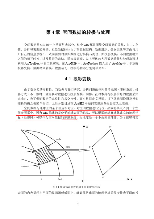
因为GIS 描述的是位于地球表面的信息,所以根据地球椭球体建立的地理坐标(经纬网)可以作为空间数据的参照系统。
而地球是一个不规则的球体,为了能够将其表面的内容显示在平面的显示器或纸面上,就必须将球面的地理坐标系统变换成平面的投图4.1椭球体表面投影到平面的微分梯形Y影坐标系统(图4.1)。
因此,运用地图投影的方法,建立地球表面和平面上点的函数关系,使地球表面上由地理坐标确定的点,在平面上有一个与它相对应的点。
地图投影的使用保证了空间信息在地域上的联系和完整性。
当系统使用的数据取自不同地图投影的图幅时,需要将一种投影的数字化数据转换为所需要投影的坐标数据。
投影转换的方法可以采用:1. 正解变换: 通过建立一种投影变换为另一种投影的严密或近似的解析关系式,直接由一种投影的数字化坐标x 、y 变换到另一种投影的直角坐标X 、Y 。
有限元等参变换的坐标转换

有限元等参变换的坐标转换英文回答:Coordinate transformation is an essential concept in finite element analysis. It allows us to express the equations of motion and other physical quantities in different coordinate systems, making it easier to analyze and solve complex problems.In the finite element method, we often work with different coordinate systems, such as global coordinates and local element coordinates. The transformation between these two coordinate systems is known as the isoparametric transformation or the finite element isoparametric mapping.The isoparametric transformation involves mapping the physical domain of an element, defined in global coordinates, to a reference domain, defined in local element coordinates. This mapping is achieved using shape functions, which are mathematical functions that describethe variation of the physical quantities within an element.To illustrate this concept, let's consider a simple example of a 2D beam element. In global coordinates, the beam is defined by its length and orientation. However, in local element coordinates, the beam is defined by its length and orientation relative to the element.When we perform a coordinate transformation, we use shape functions to map the physical coordinates of the element to the reference coordinates. These shape functions are typically polynomials that vary within the element. By applying the shape functions to the physical coordinates, we obtain the corresponding reference coordinates.Once we have the reference coordinates, we can express the physical quantities, such as displacements, strains, and stresses, in terms of the reference coordinates. This allows us to formulate the finite element equations in the reference domain, which simplifies the analysis andsolution process.In addition to the isoparametric transformation, there are other coordinate transformations that are commonly used in finite element analysis. For example, the natural coordinate system is often used to simplify the integration process when evaluating element properties, such as stiffness and mass matrices.Overall, coordinate transformation is a powerful tool in finite element analysis. It allows us to work with different coordinate systems and express physicalquantities in a more convenient and efficient manner. By understanding and applying coordinate transformations, we can effectively analyze and solve complex engineering problems.中文回答:有限元等参变换是有限元分析中的一个重要概念。
- 1、下载文档前请自行甄别文档内容的完整性,平台不提供额外的编辑、内容补充、找答案等附加服务。
- 2、"仅部分预览"的文档,不可在线预览部分如存在完整性等问题,可反馈申请退款(可完整预览的文档不适用该条件!)。
- 3、如文档侵犯您的权益,请联系客服反馈,我们会尽快为您处理(人工客服工作时间:9:00-18:30)。
Chapter2Coordinate Systems and Transformations2.1IntroductionIn navigation,guidance,and control of an aircraft or rotorcraft,there are several coordinate systems(or frames)intensively used in design and analysis(see,e.g., [171]).For ease of references,we summarize in this chapter the coordinate systems adopted in our work,which include1.the geodetic coordinate system,2.the earth-centered earth-fixed(ECEF)coordinate system,3.the local north-east-down(NED)coordinate system,4.the vehicle-carried NED coordinate system,and5.the body coordinate system.The relationships among these coordinate systems,i.e.,the coordinate transforma-tions,are also introduced.We need to point out that miniature UA V rotorcraft are normally utilized at low speeds in small regions,due to their inherent mechanical design and power limi-tation.This is crucial to some simplifications made in the coordinate transforma-tion(e.g.,omitting unimportant items in the transformation between the local NED frame and the body frame).For the same reason,partial transformation relationships provided in this chapter are not suitable for describingflight situations on the oblate rotating earth.2.2Coordinate SystemsShown in Figs.2.1and2.2are graphical interpretations of the coordinate systems mentioned above,which are to be used in sensor fusion,flight dynamics modeling,flight navigation,and control.The detailed description and definition of each of these coordinate systems are given next.G.Cai et al.,Unmanned Rotorcraft Systems,Advances in Industrial Control,23 DOI10.1007/978-0-85729-635-1_2,©Springer-Verlag London Limited2011242Coordinate Systems and Transformations Fig.2.1Geodetic,ECEF,and local NED coordinatesystemsFig.2.2Local NED,vehicle-carried NED,andbody coordinate systems2.2.1Geodetic Coordinate SystemThe geodetic coordinate system(see Fig.2.1)is widely used in GPS-based navi-gation.We note that it is not a usual Cartesian coordinate system but a system that characterizes a coordinate point near the earth’s surface in terms of longitude,lat-itude,and height(or altitude),which are respectively denoted byλ,ϕ,and h.The2.2Coordinate Systems 25longitude measures the rotational angle (ranging from −180°to 180°)between the Prime Meridian and the measured point.The latitude measures the angle (ranging from −90°to 90°)between the equatorial plane and the normal of the reference ellipsoid that passes through the measured point.The height (or altitude)is the local vertical distance between the measured point and the reference ellipsoid.It should be noted that the adopted geodetic latitude differs from the usual geocentric lati-tude (ϕ ),which is the angle between the equatorial plane and a line from the mass center of the stly,we note that the geocentric latitude is not used in our work.Coordinate vectors expressed in terms of the geodetic frame are denoted with a subscript g,i.e.,the position vector in the geodetic coordinate system is denoted by P g = λϕh.(2.1)Important parameters associated with the geodetic frame include1.the semi-major axis R E a ,2.the flattening factor f ,3.the semi-minor axis R E b ,4.the first eccentricity e ,5.the meridian radius of curvature M E ,and6.the prime vertical radius of curvature N E .These parameters are either defined (items 1and 2)or derived (items 3to 6)based on the WGS 84(world geodetic system 84,which was originally proposed in 1984and lastly updated in 2004[212])ellipsoid model.More specifically,we haveR E a =6,378,137.0m ,(2.2)f =1/298.257223563,(2.3)R E b =R E a (1−f )=6,356,752.0m ,(2.4)e = R 2E a −R 2E b R E a=0.08181919,(2.5)M E =R E a (1−e 2)(1−e 2sin 2ϕ)3/2,(2.6)N E =R E a 1−e 2sin 2ϕ.(2.7)2.2.2Earth-Centered Earth-Fixed Coordinate SystemThe ECEF coordinate system rotates with the earth around its spin axis.As such,a fixed point on the earth surface has a fixed set of coordinates (see,e.g.,[202]).The origin and axes of the ECEF coordinate system (see Fig.2.1)are defined as follows:262Coordinate Systems and Transformations1.The origin (denoted by O e )is located at the center of the earth.2.The Z-axis (denoted by Z e )is along the spin axis of the earth,pointing to the north pole.3.The X-axis (denoted by X e )intersects the sphere of the earth at 0°latitude and 0°longitude.4.The Y-axis (denoted by Y e )is orthogonal to the Z-and X-axes with the usual right-hand rule.Coordinate vectors expressed in the ECEF frame are denoted with a subscript e.Similar to the geodetic system,the position vector in the ECEF frame is denoted by P e = x ey e z e.(2.8)2.2.3Local North-East-Down Coordinate SystemThe local NED coordinate system is also known as a navigation or ground coordi-nate system.It is a coordinate frame fixed to the earth’s surface.Based on the WGS 84ellipsoid model,its origin and axes are defined as the following (see also Figs.2.1and 2.2):1.The origin (denoted by O n )is arbitrarily fixed to a point on the earth’s surface.2.The X-axis (denoted by X n )points toward the ellipsoid north (geodetic north).3.The Y-axis (denoted by Y n )points toward the ellipsoid east (geodetic east).4.The Z-axis (denoted by Z n )points downward along the ellipsoid normal.The local NED frame plays a very important role in flight control and navigation.Navigation of small-scale UA V rotorcraft is normally carried out within this frame.Coordinate vectors expressed in the local NED coordinate system are denoted with a subscript n.More specifically,the position vector,P n ,the velocity vector,V n ,and the acceleration vector,a n ,of the NED coordinate system are adopted and are,respectively,defined as P n = x n y n z n ,V n = u n v n w n ,a n = a x ,na y ,n a z ,n.(2.9)We also note that in our work,we normally select the takeoff point,which is also the sensor initialization point,in each flight test as the origin of the local NED frame.When it is clear in the context,we also use the following definition throughout the monograph for the position vector in the local NED frame,P n = xy z.(2.10)Furthermore,h =−z is used to denote the actual height of the unmanned system.2.2Coordinate Systems27 2.2.4Vehicle-Carried North-East-Down Coordinate SystemThe vehicle-carried NED system is associated with theflying vehicle.Its origin and axes(see Fig.2.2)are given by the following:1.The origin(denoted by O nv)is located at the center of gravity(CG)of theflyingvehicle.2.The X-axis(denoted by X nv)points toward the ellipsoid north(geodetic north).3.The Y-axis(denoted by Y nv)points toward the ellipsoid east(geodetic east).4.The Z-axis(denoted by Z nv)points downward along the ellipsoid normal.Strictly speaking,the axis directions of the vehicle-carried NED frame vary with respect to theflying-vehicle movement and are thus not aligned with those of the local NED frame.However,as mentioned earlier,the miniature rotorcraft UA Vsfly only in a small region with low speed,which results in the directional difference being completely neglectable.As such,it is reasonable to assume that the directions of the vehicle-carried and local NED coordinate systems constantly coincide with each other.Coordinate vectors expressed in the vehicle-carried NED frame are denoted with a subscript nv.More specifically,the velocity vector,V nv,and the acceleration vec-tor,a nv,of the vehicle-carried NED coordinate system are adopted and are,respec-tively,defined asV nv= unvv nvw nv,a nv=ax,nva y,nva z,nv.(2.11)2.2.5Body Coordinate SystemThe body coordinate system is vehicle-carried and is directly defined on the body of theflying vehicle.Its origin and axes(see Fig.2.2)are given by the following:1.The origin(denoted by O b)is located at the center of gravity(CG)of theflyingvehicle.2.The X-axis(denoted by X b)points forward,lying in the symmetric plane of theflying vehicle.3.The Y-axis(denoted by Y b)is starboard(the right side of theflying vehicle).4.The Z-axis(denoted by Z b)points downward to comply with the right-hand rule. Coordinate vectors expressed in the body frame are appended with a subscript b. Next,we defineV b= uvw(2.12)282Coordinate Systems and Transformations to be the vehicle-carried NED velocity,i.e.,V nv ,projected onto the body frame,and a b = a xa y a z(2.13)to be the vehicle-carried NED acceleration,i.e.,a nv ,projected onto the body frame.These two vectors are intensively used in capturing the 6-DOF rigid-body dynamics of unmanned systems.2.3Coordinate TransformationsThe transformation relationships among the adopted coordinate frames are intro-duced in this section.We first briefly introduce some fundamental knowledge related to Cartesian-frame transformations before giving the detailed coordinate transfor-mations.2.3.1Fundamental KnowledgeWe summarize in this subsection the basic concepts of the Euler rotation and rotation matrix,Euler angles,and angular velocity vector used in flight modeling,control and navigation.2.3.1.1Euler RotationsThe orientation of one Cartesian coordinate system with respect to another can al-ways be described by three successive Euler rotations [171].For aerospace appli-cation,the Euler rotations perform about each of the three Cartesian axes conse-quently,following the right-hand rule.Shown in Fig.2.3is a simple example,in which Frames C1and C2are two Cartesian systems with the aligned Z-axes point-ing toward us.We take Frame C2as the reference and can obtain Frame C1through a Euler rotation (by rotating Frame C2counter-clockwise with an angle of ξ).Then,it is straightforward to verify that the position vectors of any given point expressed in Frame C1,say P C1,and in Frame C2,say P C2,are related byP C1=R C1/C2P C2,(2.14)where R C1/C2is defined as a rotation matrix that transforms the vector P from FrameC2to Frame C1and is given as R C1/C2= cos ξsin ξ0−sin ξcos ξ0001.(2.15)It is simple to show thatR C2/C1=R −1C1/C2=R T C1/C2.(2.16)2.3Coordinate Transformations29 Fig.2.3Illustration of aEuler rotation2.3.1.2Euler AnglesThe Euler angles are three angles introduced by Euler to describe the orientation of a rigid body.Although the relative orientation between any two Cartesian frames can be described by Euler angles,we focus in this monograph merely on the transforma-tion between the vehicle-carried(or the local)NED and the body frames,following a particular rotation sequence.More specifically,the adopted Euler angles move the reference frame to the referred frame,following a Z-Y-X(or the so-called3–2–1) rotation sequence.These three Euler angles are also known as the yaw(or heading), pitch,and roll angles,which are defined as the following(see Fig.2.4for graphical illustration):1.Y AW ANGLE,denoted byψ,is the angle from the vehicle-carried NED X-axis tothe projected vector of the body X-axis on the X-Y plane of the vehicle-carried NED frame.The right-handed rotation is about the vehicle-carried NED Z-axis.After this rotation(denoted by R int1/nv),the vehicle-carried NED frame transfers to a once-rotated intermediate frame.2.P ITCH ANGLE,denoted byθ,is the angle from the X-axis of the once-rotatedintermediate frame to the body frame X-axis.The right-handed rotation is about the Y-axis of the once-rotated intermediate frame.After this rotation(denoted by R int2/int1),we have a twice-rotated intermediate frame whose X-axis coincides with the X-axis of the body frame.3.R OLL ANGLE,denoted byφ,is the angle from the Y-axis(or Z-axis)of the twice-rotated intermediate frame to that of the body frame.This right-handed rotation (denoted by R b/int2)is about the X-axis of the twice-rotated intermediate frame (or the body frame).302Coordinate Systems andTransformations Fig.2.4Euler angles and yaw-pitch-roll rotation sequenceThe three relative rotation matrices are respectively given byR int1/nv = cos ψsin ψ0−sin ψcos ψ0001 ,(2.17)R int2/int1= cos θ0−sin θ010sin θ0cos θ ,(2.18)andR b /int2= 1000cos φsin φ0−sin φcos φ .(2.19)2.3Coordinate Transformations 312.3.1.3Angular VelocitiesThe angular velocities (or angular rates)are associated with the relative motion be-tween two coordinate systems.Considering that Frame C1is rotating with respect to Frame C2,the angular velocity is denoted by ω∗C1/C2= ωx ωy ωz,(2.20)where ∗is a coordinate frame on which the angular velocity vector is projected.We note that the coordinate frame ∗can be C1or C2or any another frame.It is simple to verify that the angular velocity vector of Frame C2rotating with respect to Frame C1is given byω∗C2/C1=−ω∗C1/C2.(2.21)2.3.2Coordinate TransformationsWe proceed to present the necessary coordinate transformations among the coordi-nate systems adopted,of which the first three transformations are mainly employed for rotorcraft spatial navigation,the fourth one is commonly adopted for flight con-trol purposes,and finally,the last one focuses on an approximation particularly suit-able for the miniature rotorcraft.2.3.2.1Geodetic and ECEF Coordinate SystemsThe position vector transformation from the geodetic system to the ECEF coordinate system is an intermediate step in converting the GPS position measurement to the local NED coordinate system.Given a point in the geodetic system,say P g = λϕh,its coordinate in the ECEF frame is given by P e = x e y e z e = (N E +h)cos ϕcos λ(N E +h)cos ϕsin λ[N E (1−e 2)+h ]sin ϕ,(2.22)where e and N E are as given in (2.5)and (2.7),respectively.2.3.2.2ECEF and Local NED Coordinate SystemsThe position transformation from the ECEF frame to the local NED frame is re-quired together with the transformation from the geodetic system to the ECEF frame322Coordinate Systems and Transformations to form a complete position conversion from the geodetic to local NED frames.More specifically,we haveP n =R n /e (P e −P e ,ref ),(2.23)where P e ,ref is the position of the origin of the local NED frame (i.e.,O n ,normally the takeoff point in UA V applications)in the ECEF coordinate system,and R n /e is the rotation matrix from the ECEF frame to the local NED frame,which is given by R n /e = −sin ϕref cos λref −sin ϕref sin λref cos ϕref −sin λref cos λref 0−cos ϕref cos λref −cos ϕref sin λref −sin ϕref,(2.24)and where λref and ϕref are the geodetic longitude and latitude corresponding to P e ,ref .2.3.2.3Geodetic and Vehicle-Carried NED Coordinate SystemsIn aerospace navigation,a kinematical relationship between geodetic position and vehicle-carried NED velocity is of great importance.The derivative of the geode-tic position can be expressed in terms of the vehicle-carried NED velocity as the following:˙λ=v nv (N E ,(2.25)˙ϕ=u nv M E ,(2.26)and˙h =−w nv .(2.27)We note that the first two equations are derived based on spherical triangles,whereas the third one can be easily obtained from the definitions of h and w nv .The derivatives of the vehicle-carried NED velocities are respectively given by˙u nv =−v 2nv sin ϕ(N E +h)cos ϕ+u nv w nv M E +h+a mx ,nv ,(2.28)˙v nv =u nv v nv sin ϕ(N E +v nv w nv N E +a my ,nv ,(2.29)and˙w nv =−v 2nv N E −u 2nv M E +g +a mz ,nv ,(2.30)where g is the gravitational acceleration,and a mea ,nv = a mx ,nva my ,nva mz ,nv (2.31)2.3Coordinate Transformations33 is the projection of a mea,b,the proper acceleration measured on the body frame,onto the vehicle-carried NED frame.The proper acceleration is an acceleration relative to a free-fall observer who is momentarily at rest relative to the object being measured [209].In the above equations,we omit terms related to the earth’s self-rotation, which is reasonable for small-scale UA V rotorcraft working in a small confined area.2.3.2.4Vehicle-Carried NED and Body Coordinate SystemsKinematical relationships between the vehicle-carried NED and the body frames are important toflight dynamics modeling and automaticflight control.For translational kinematics,we haveV b=R b/nv V nv,(2.32)a b=R b/nv a nv,(2.33) anda mea,b=R b/nv a mea,nv,(2.34) where R b/nv is the rotation matrix from the vehicle-carried NED frame to the body frame and is given byR b/nv= cθcψcθsψ−sθsφsθcψ−cφsψsφsθsψ+cφcψsφcθcφsθcψ+sφsψcφsθsψ−sφcψcφcθ,(2.35)and where s∗and c∗denote sin(∗)and cos(∗),respectively.For rotational kinematics,we focus on the angular velocity vectorωb b/nv,which describes the rotation of the vehicle-carried NED frame with respect to the body frame projected onto the body frame.Following the definition and sequence of the Euler angles,it can be expressed asωb b/nv:= pqr=˙φ+R b/int2˙θ+R int2/int1˙ψ=S ˙φ˙θ˙ψ,(2.36)where p,q,and r are the standard symbols adopted in the aerospace community for the components ofωb b/nv,R int2/int1and R b/int2are respectively given as in(2.18) and(2.19),and lastly,S is the lumped transformation matrix given byS= 10−sinθ0cosφsinφcosθ0−sinφcosφcosθ.(2.37)342Coordinate Systems and TransformationsIt is simple to verify thatS−1= 1sinφtanθcosφtanθ0cosφ−sinφ0sinφ/cosθcosφ/cosθ.(2.38)We note that(2.36)is known as the Euler kinematical equation and thatθ=±90°causes singularity in(2.37),which can be avoided by using quaternion expressions.2.3.2.5Local and Vehicle-Carried NED Coordinate FramesAs mentioned in Sect.2.2.4,under the assumption that there is no directional differ-ence between the local and vehicle-carried NED frames,we haveV n=V nv,ωb b/n=ωb b/nv,a n=a nv,a mea,n=a mea,nv,(2.39) where a mea,n is the projection of the proper acceleration measured on the body frame,i.e.,a mea,b,onto the local NED frame.These properties will be used through-out the entire monograph./978-0-85729-634-4。