机器学习十大算法:CART
决策树 cart最佳分割点算法
决策树是一种经典的机器学习算法,它通过对数据集进行分割来构建一个预测模型。
在决策树的构建过程中,寻找最佳的分割点是非常重要的一步。
CART(Classification and Regression Trees)是一种常用的决策树算法,它使用基尼系数来确定最佳的分割点。
本文将重点介绍CART最佳分割点算法的原理和实现方法。
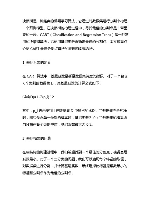
1. 基尼系数的定义在CART算法中,基尼系数是衡量数据集纯度的指标。
对于一个包含K个类别的数据集D,其基尼系数的计算公式如下:Gini(D)=1-Σ(p_i)^2其中,p_i 表示类别 i 在数据集 D 中所占的比例。
当数据集完全纯净时,即只包含单一类别的样本时,基尼系数为 0;当数据集的样本均匀分布在各个类别中时,基尼系数最大为 0.5。
2. 基尼指数的计算在决策树的构建过程中,我们希望找到一个最佳的分割点,使得基尼系数最小。
对于一个二分类的问题,我们可以遍历每个特征的取值,对数据集进行分割,并计算基尼系数。
最终选择使得基尼系数最小的特征和分割点作为最佳的分割点。
3. CART最佳分割点算法CART算法使用递归二分来构建决策树,其最佳分割点算法基本流程如下:1. 遍历每个特征的取值,对数据集进行分割;2. 计算每个分割点的基尼系数;3. 选择使得基尼系数最小的特征和分割点作为最佳的分割点;4. 重复以上步骤,直至满足停止条件(如树的最大深度、节点的最小样本数等)。
4. 实现方法在实际应用中,我们可以使用贪心算法来寻找最佳的分割点。
具体实现方法如下:1. 对于每个特征,对其取值进行排序;2. 遍历每个特征的取值,使用一个指针来指示当前的分割点;3. 维护一个变量来存储当前的基尼系数最小值,以及相应的特征和分割点;4. 在遍历过程中,不断更新基尼系数最小值和最佳的特征和分割点;5. 最终得到使得基尼系数最小的特征和分割点作为最佳的分割点。
5. 结语CART最佳分割点算法是决策树构建过程中的关键步骤,通过有效地寻找最佳的分割点,可以构建出具有良好泛化能力的决策树模型。
经典算法CART

经典算法CARTCART(Classification And Regression Trees)是一种经典的算法,用于建立分类和回归树模型。
它是由Leo Breiman在1984年首次提出的,目前被广泛应用于数据挖掘和机器学习领域。
CART算法基于决策树的思想,可以将输入数据集分割成多个小的子集,每个子集代表一个决策树节点。
通过对特征的选择和分割,可以使得每个子集的纯度更高,即同一类别的样本更多。
最终,CART算法会生成一棵满足纯度要求的决策树模型。
CART算法的主要步骤如下:1. 特征选择:CART算法使用其中一种准则来选择最佳的特征。
常用的准则包括基尼指数(Gini index)和信息增益(information gain)。
基尼指数衡量了数据集的不纯度,而信息增益衡量了特征对数据集纯度的贡献程度。
选择具有最大基尼指数或信息增益的特征作为当前节点的划分特征。
2.划分数据集:根据划分特征的取值将数据集分成多个子集。
对于离散特征,每个取值对应一个子集;对于连续特征,可以选择一个划分点将数据集分成两个子集。
3.递归建立子树:对每个子集,重复步骤1和步骤2,递归地建立子树。
直到达到停止条件,例如达到最大深度或纯度要求。
4.剪枝处理:为了避免过拟合,CART算法会对生成的决策树进行剪枝处理。
根据其中一种评估准则,剪去部分子树或合并子树。
CART算法具有一些优点,使得它成为一种经典的算法。
首先,CART算法可以处理离散特征和连续特征,非常灵活。
其次,CART算法生成的决策树易于理解和解释,可以用于预测和决策解释。
此外,CART算法还能处理多分类和回归问题。
然而,CART算法也存在一些限制。
首先,CART算法只能生成二叉树,即每个节点只有两个分支。
这可能会导致决策树过于复杂,需要更多的分支来表示复杂的决策边界。
其次,CART算法在处理高维数据和数据不平衡的情况下可能会遇到困难,需要进行特殊处理。
总结起来,CART算法是一种经典的算法,用于建立分类和回归树模型。
CART算法介绍

CART算法介绍CART(Classification And Regression Trees)算法是一种机器学习算法,主要用于决策树模型的构建。
CART算法通过递归地将数据集分割成多个子集,直到子集中的数据只属于同一类别或满足一些预定义的条件。
CART算法可以用于分类和回归问题。
1.选择一个初始特征作为根节点,并将数据集分成两个子集。
选择初始特征的方法有很多,常见的方法有基尼指数和信息增益。
2.对每个子集,重复步骤1,选择一个最佳特征并将子集分割成更小的子集。
分割策略可以采用相同的方法,即最小化基尼指数或最大化信息增益。
3.递归地重复上述步骤,生成一棵完整的决策树,其中每个叶子节点代表一个类别。
4.进行剪枝操作,可以通过最小化损失函数或使用交叉验证方法来选择最优的决策树。
1.算法简单易懂,实现较为容易。
CART算法将复杂的决策问题简化为“是”和“否”的问题,其结果容易解释和理解。
2.可以处理多类别问题。
CART算法可以应用于多类别分类问题,并且可以通过增加决策树的深度来提高分类的准确性。
3.能够处理非线性特征。
CART算法对非线性特征没有太强的限制,可以处理多种类型的特征。
4.对缺失值和异常值具有较好的鲁棒性。
CART算法对于缺失值和异常值有一定的容忍程度,不会对模型产生太大的影响。
然而,CART算法也存在一些不足之处:1.对于样本噪声比较敏感。
CART算法对于噪声数据比较敏感,噪声数据容易导致树模型产生过拟合的情况。
2.对于类别不平衡的数据集效果不佳。
CART算法对于类别不平衡的数据集容易出现偏倚现象,导致模型效果下降。
3.容易产生过拟合。
CART算法在构建决策树时采用了贪心策略,很容易产生过拟合问题。
为了避免过拟合,可以进行剪枝操作。
总结来说,CART算法是一种强大且灵活的机器学习算法,适用于分类和回归问题。
它具有较好的鲁棒性和解释性,并且能够处理多类别和非线性特征。
然而,CART算法仍然存在一些限制,如对噪声敏感和对类别不平衡的数据处理能力不足。
机器学习10大经典算法详解

机器学习10⼤经典算法详解本⽂为⼤家分享了机器学习10⼤经典算法,供⼤家参考,具体内容如下1、C4.5C4.5算法是机器学习算法中的⼀种分类决策树算法,其核⼼算法是ID3算法. C4.5算法继承了ID3算法的优点,并在以下⼏⽅⾯对ID3算法进⾏了改进:1)⽤信息增益率来选择属性,克服了⽤信息增益选择属性时偏向选择取值多的属性的不⾜;2)在树构造过程中进⾏剪枝;3)能够完成对连续属性的离散化处理;4)能够对不完整数据进⾏处理。
C4.5算法有如下优点:产⽣的分类规则易于理解,准确率较⾼。
其缺点是:在构造树的过程中,需要对数据集进⾏多次的顺序扫描和排序,因⽽导致算法的低效。
2、The k-means algorithm即K-Means算法k-means algorithm算法是⼀个聚类算法,把n的对象根据他们的属性分为k个分割,k < n。
它与处理混合正态分布的最⼤期望算法很相似,因为他们都试图找到数据中⾃然聚类的中⼼。
它假设对象属性来⾃于空间向量,并且⽬标是使各个群组内部的均⽅误差总和最⼩。
3、Support vector machines⽀持向量机⽀持向量机(Support Vector Machine),简称SV机(论⽂中⼀般简称SVM)。
它是⼀种监督式学习的⽅法,它⼴泛的应⽤于统计分类以及回归分析中。
⽀持向量机将向量映射到⼀个更⾼维的空间⾥,在这个空间⾥建⽴有⼀个最⼤间隔超平⾯。
在分开数据的超平⾯的两边建有两个互相平⾏的超平⾯。
分隔超平⾯使两个平⾏超平⾯的距离最⼤化。
假定平⾏超平⾯间的距离或差距越⼤,分类器的总误差越⼩。
⼀个极好的指南是C.J.C Burges的《模式识别⽀持向量机指南》。
van der Walt和Barnard 将⽀持向量机和其他分类器进⾏了⽐较。
4、The Apriori algorithmApriori算法是⼀种最有影响的挖掘布尔关联规则频繁项集的算法。
其核⼼是基于两阶段频集思想的递推算法。
大数据经典算法CART讲解

大数据经典算法CART讲解CART(分类与回归树)是一种经典的机器学习算法,用于解决分类和回归问题。
它是由Leo Breiman等人在1984年提出的,是决策树算法的一种改进和扩展。
CART算法的核心思想是通过将输入空间划分为多个区域来构建一棵二叉树,每个区域用于表示一个决策规则。
CART算法的整个过程可以分为两个部分:生成和剪枝。
在生成阶段,CART算法通过递归地将数据集切分为两个子集,直到满足一些停止条件。
在剪枝阶段,CART算法通过剪枝策略对生成的树进行剪枝,以防止过拟合。
生成阶段中,CART算法的切分准则是基于Gini系数的。
Gini系数衡量了将数据集切分为两个子集后的不纯度,即数据集中样本不属于同一类别的程度。
CART算法通过选择Gini系数最小的切分点来进行切分,使得切分后的两个子集的纯度最高。
剪枝阶段中,CART算法通过损失函数来评估子树的贡献。
损失函数考虑了子树的拟合程度和子树的复杂度,以平衡模型的拟合能力和泛化能力。
剪枝阶段的目标是找到一个最优的剪枝点,使得剪枝后的子树的整体损失最小。
CART算法具有许多优点。
首先,CART算法可以处理多类别问题,不需要进行额外的转换。
其次,CART算法能够处理混合类型的数据,比如同时具有连续型和离散型特征的数据。
此外,CART算法能够处理缺失数据,并能够自动选择缺失数据的处理方法。
最后,CART算法生成的模型具有很好的可解释性,可以直观地理解决策过程。
然而,CART算法也存在一些不足之处。
首先,CART算法是一种贪心算法,通过局部最优来构建模型,不能保证全局最优。
其次,CART算法对输入特征的顺序敏感,不同的特征顺序可能会导致不同的模型结果。
此外,CART算法对噪声和异常值很敏感,可能会导致过拟合。
在实际应用中,CART算法广泛应用于分类和回归问题。
在分类问题中,CART算法可以用于构建决策树分类器,对样本进行分类预测。
在回归问题中,CART算法可以用于构建决策树回归器,根据输入特征预测输出值。
cart算法

cart算法
cart算法,全称Classification and Regression Trees,即分类与回归树算法,是一种基于决策树的机器学习算法。
cart算法可以用于分类问题和回归问题。
在分类问题中,cart算法根据特征值将数据集划分为多个子集,并通过选择一个最佳划分特征和划分阈值来构建决策树。
在回归问题中,cart算法根据特征值将数据集划分为多个子集,并通过选择一个最佳划分特征和划分阈值来构建回归树。
cart算法的核心思想是通过递归地选择最佳划分特征和划分阈值来构建决策树。
在每个节点上,通过计算基于当前特征和划分阈值的Gini指数(用于分类问题)或平方误差(用于回归问题)来评估划分的好坏,选择最小的Gini指数或平方误差对应的特征和划分阈值进行划分。
划分后的子集继续递归地进行划分,直到满足停止条件(如节点中的样本数小于预设阈值或达到最大深度为止),然后生成叶子节点并赋予相应的类别标签或回归值。
cart算法具有较好的拟合能力和可解释性,可以处理混合类型的特征和缺失值。
然而,cart算法容易过拟合,需要采取剪枝操作或加入正则化项来降低模型复杂度。
可以通过使用不同的评估标准和剪枝策略来改进cart算法,如基于信息增益、基尼系数、均方差等评估标准和预剪枝、后剪枝等剪枝
策略。
此外,也可以使用集成学习方法(如随机森林、梯度提升树)来进一步提高模型的性能。
大数据经典算法CART_讲解资料

大数据经典算法CART_讲解资料CART算法,即分类与回归树(Classification and Regression Tree)算法,是一种经典的应用于大数据分析的算法。
它将数据集按照特征属性进行划分,然后根据各个特征属性的分割点将数据集划分为多个子集,进而得到一个树形的划分结构。
通过分析划分特征和划分点的选择,CART算法能够高效地解决分类和回归问题。
对于分类问题,CART算法通过衡量不纯度(impurity)来选择划分特征和划分点。
常用的不纯度指标包括基尼指数(Gini index)和信息增益(information gain)。
基尼指数衡量了随机从一个样本集合中抽取两个样本,其中属于不同类别的概率;信息增益则使用熵(entropy)作为不纯度的度量标准。
CART算法会选择使得划分后的子集的纯度提升最大的特征属性和相应的划分点进行划分。
对于回归问题,CART算法通过最小化划分后的子集的方差来选择划分特征和划分点。
在每个内部节点上,CART算法选择使得划分后的子集的方差最小化的特征属性和相应的划分点进行划分。
CART算法的优点在于它能够处理高维数据和有缺失值的数据,具有较强的鲁棒性。
此外,CART算法构建的决策树具有可解释性,能够提供对数据的直观理解。
同时,CART算法还能处理不平衡类别数据和多类别问题。
然而,CART算法也存在一些不足之处。
首先,CART算法是一种局部最优算法,可能会陷入局部最优解而无法达到全局最优解。
其次,CART 算法不适用于处理连续型特征属性,需要对连续特征进行离散化处理。
此外,由于CART算法是自顶向下的贪心算法,因此容易过拟合,需要采用一些剪枝策略进行模型的修剪。
在实际应用中,为了提高CART算法的性能,可以使用集成学习方法如随机森林、梯度提升树等。
这些方法通过构建多个CART模型,并通过集成的方式来提高预测准确率和鲁棒性。
总结起来,CART算法是一种经典的大数据分析算法,适用于解决分类和回归问题。
CART算法

这(2)里计输算样入本标集题D的文基字尼系数,如果基尼系数小于阈值,则返回决策树子树,当前节点停止
递归。 (3)计算当前节点现ቤተ መጻሕፍቲ ባይዱ的各个特征的各个特征值对数据集D的基尼系数,对于离散值和连续
值的处理方法和基尼系数的计算见第二节。缺失值的处理方法和C4.5算法里描述的相同。 (4)在计算出来的各个特征的各个特征值对数据集D的基尼系数中,选择基尼系数最小的特
剪枝损失函数表达式:
α为正则化参数(和线性回归的正则化一样),C(Tt)为训练数据的预测误差,|Tt|是子树T叶 子节点数量。
当α = 0时,即没有正则化,原始生成的CART树即为最优子树。当α= ∞时,正则化强 度最大,此时由原始的生成CART树的根节点组成的单节点树为最优子树。当然,这是两种 极端情况,一般来说,α越大,剪枝剪的越厉害,生成的最优子树相比原生决策树就越偏小。 对于固定的α,一定存在使得损失函数Cα(Tt)最小的唯一子树。
CART既能是分类树,又能是 回归树。
如果我们想预测一个人是否 已婚,那么构建的CART将是分类 树,其叶子节点的输出结果为一个 实际的类别,在这个例子里是婚姻 的情况(已婚或者未婚),选择叶 子节点中数量占比最大的类别作为 输出的类别。
如果想预测一个人的年龄, 那么构建的将是回归树,预测用户 的实际年龄,是一个具体的输出值。 怎样得到这个输出值?一般情况下 选择使用中值、平均值或者众数进 行表示。
04 CART树算法的剪枝
剪枝的思路: 对于位于节点t的任意一颗子树Tt,如果没有剪枝,损失函数是:
如果将其剪掉,仅保留根节点,损失函数是:Cα(T)= C(T)+ α 当α= 0或α很小,Cα(Tt) < Cα(T),当α增大到一定程度时 Cα(Tt) = Cα(T) 当α继续增大时不等式反向,即满足下式:
- 1、下载文档前请自行甄别文档内容的完整性,平台不提供额外的编辑、内容补充、找答案等附加服务。
- 2、"仅部分预览"的文档,不可在线预览部分如存在完整性等问题,可反馈申请退款(可完整预览的文档不适用该条件!)。
- 3、如文档侵犯您的权益,请联系客服反馈,我们会尽快为您处理(人工客服工作时间:9:00-18:30)。
Chapter10CART:Classification and Regression Trees Dan SteinbergContents10.1Antecedents (180)10.2Overview (181)10.3A Running Example (181)10.4The Algorithm Briefly Stated (183)10.5Splitting Rules (185)10.6Prior Probabilities and Class Balancing (187)10.7Missing Value Handling (189)10.8Attribute Importance (190)10.9Dynamic Feature Construction (191)10.10Cost-Sensitive Learning (192)10.11Stopping Rules,Pruning,Tree Sequences,and Tree Selection (193)10.12Probability Trees (194)10.13Theoretical Foundations (196)10.14Post-CART Related Research (196)10.15Software Availability (198)10.16Exercises (198)References (199)The1984monograph,“CART:Classification and Regression Trees,”coauthored by Leo Breiman,Jerome Friedman,Richard Olshen,and Charles Stone(BFOS),repre-sents a major milestone in the evolution of artificial intelligence,machine learning, nonparametric statistics,and data mining.The work is important for the compre-hensiveness of its study of decision trees,the technical innovations it introduces,its sophisticated examples of tree-structured data analysis,and its authoritative treatment of large sample theory for trees.Since its publication the CART monograph has been cited some3000times according to the science and social science citation indexes; Google Scholar reports about8,450citations.CART citations can be found in almost any domain,with many appearing infields such as credit risk,targeted marketing,fi-nancial markets modeling,electrical engineering,quality control,biology,chemistry, and clinical medical research.CART has also strongly influenced image compression179180CART:Classification and Regression Treesvia tree-structured vector quantization.This brief account is intended to introduce CART basics,touching on the major themes treated in the CART monograph,and to encourage readers to return to the rich original source for technical details,discus-sions revealing the thought processes of the authors,and examples of their analytical style.10.1AntecedentsCART was not thefirst decision tree to be introduced to machine learning,although it is thefirst to be described with analytical rigor and supported by sophisticated statistics and probability theory.CART explicitly traces its ancestry to the auto-matic interaction detection(AID)tree of Morgan and Sonquist(1963),an automated recursive method for exploring relationships in data intended to mimic the itera-tive drill-downs typical of practicing survey data analysts.AID was introduced as a potentially useful tool without any theoretical foundation.This1960s-era work on trees was greeted with profound skepticism amidst evidence that AID could radically overfit the training data and encourage profoundly misleading conclusions(Einhorn, 1972;Doyle,1973),especially in smaller samples.By1973well-read statisticians were convinced that trees were a dead end;the conventional wisdom held that trees were dangerous and unreliable tools particularly because of their lack of a theoretical foundation.Other researchers,however,were not yet prepared to abandon the tree line of thinking.The work of Cover and Hart(1967)on the large sample properties of nearest neighbor(NN)classifiers was instrumental in persuading Richard Olshen and Jerome Friedman that trees had sufficient theoretical merit to be worth pursu-ing.Olshen reasoned that if NN classifiers could reach the Cover and Hart bound on misclassification error,then a similar result should be derivable for a suitably constructed tree because the terminal nodes of trees could be viewed as dynami-cally constructed NN classifiers.Thus,the Cover and Hart NN research was the immediate stimulus that persuaded Olshen to investigate the asymptotic properties of trees.Coincidentally,Friedman’s algorithmic work on fast identification of nearest neighbors via trees(Friedman,Bentley,and Finkel,1977)used a recursive partition-ing mechanism that evolved into CART.One predecessor of CART appears in the 1975Stanford Linear Accelerator Center(SLAC)discussion paper(Friedman,1975), subsequently published in a shorter form by Friedman(1977).While Friedman was working out key elements of CART at SLAC,with Olshen conducting mathemat-ical research in the same lab,similar independent research was under way in Los Angeles by Leo Breiman and Charles Stone(Breiman and Stone,1978).The two separate strands of research(Friedman and Olshen at Stanford,Breiman and Stone in Los Angeles)were brought together in1978when the four CART authors for-mally began the process of merging their work and preparing to write the CART monograph.10.3A Running Example18110.2OverviewThe CART decision tree is a binary recursive partitioning procedure capable of pro-cessing continuous and nominal attributes as targets and predictors.Data are handled in their raw form;no binning is required or recommended.Beginning in the root node,the data are split into two children,and each of the children is in turn split into grandchildren.Trees are grown to a maximal size without the use of a stopping rule; essentially the tree-growing process stops when no further splits are possible due to lack of data.The maximal-sized tree is then pruned back to the root(essentially split by split)via the novel method of cost-complexity pruning.The next split to be pruned is the one contributing least to the overall performance of the tree on training data(and more than one split may be removed at a time).The CART mechanism is intended to produce not one tree,but a sequence of nested pruned trees,each of which is a candidate to be the optimal tree.The“right sized”or“honest”tree is identified by evaluating the predictive performance of every tree in the pruning sequence on inde-pendent test data.Unlike C4.5,CART does not use an internal(training-data-based) performance measure for tree selection.Instead,tree performance is always measured on independent test data(or via cross-validation)and tree selection proceeds only af-ter test-data-based evaluation.If testing or cross-validation has not been performed, CART remains agnostic regarding which tree in the sequence is best.This is in sharp contrast to methods such as C4.5or classical statistics that generate preferred models on the basis of training data measures.The CART mechanism includes(optional)automatic class balancing and auto-matic missing value handling,and allows for cost-sensitive learning,dynamic feature construction,and probability tree estimation.Thefinal reports include a novel at-tribute importance ranking.The CART authors also broke new ground in showing how cross-validation can be used to assess performance for every tree in the pruning sequence,given that trees in different cross-validation folds may not align on the number of terminal nodes.It is useful to keep in mind that although BFOS addressed all these topics in the1970s,in some cases the BFOS treatment remains the state-of-the-art.The literature of the1990s contains a number of articles that rediscover core insightsfirst introduced in the1984CART monograph.Each of these major features is discussed separately below.10.3A Running ExampleTo help make the details of CART concrete we illustrate some of our points using an easy-to-understand real-world example.(The data have been altered to mask some of the original specifics.)In the early1990s the author assisted a telecommunications company in understanding the market for mobile phones.Because the mobile phone182CART:Classification and Regression TreesTABLE10.1Example Data Summary StatisticsAttribute N N Missing%Missing N Distinct Mean Min Max AGE81318 2.29 5.05919 CITY830005 1.76915 HANDPRIC830004145.360235 MARITAL8229 1.13 1.901513 PAGER82560.7220.07636401 RENTHOUS830003 1.790613 RESPONSE8300020.151801 SEX81912 1.42 1.443212 TELEBILC768637.6654.1998116 TRA VTIME651180225 2.31815 USEPRICE83000411.1511030 MARITAL=Marital Status(Never Married,Married,Divorced/Widowed)TRA VTIME=estimated commute time to major center of employmentAGE is recorded as an integer ranging from1to9was a new technology at that time,we needed to identify the major drivers of adoption of this then-new technology and to identify demographics that might be related to price sensitivity.The data consisted of a household’s response(yes/no)to a market test offer of a mobile phone package;all prospects were offered an identical package of a handset and service features,with one exception that the pricing for the package was varied randomly according to an experimental design.The only choice open to the households was to accept or reject the offer.A total of830households were approached and126of the households agreed to subscribe to the mobile phone service plan.One of our objectives was to learn as much as possible about the differences between subscribers and nonsubscribers.A set of summary statistics for select attributes appear in Table10.1.HANDPRIC is the price quoted for the mobile handset,USEPRIC is the quoted per-minute charge,and the other attributes are provided with common names.A CART classification tree was grown on these data to predict the RESPONSE attribute using all the other attributes as predictors.MARITAL and CITY are cate-gorical(nominal)attributes.A decision tree is grown by recursively partitioning the training data using a splitting rule to identify the split to use at each node.Figure10.1 illustrates this process beginning with the root node splitter at the top of the tree. The root node at the top of the diagram contains all our training data,including704 nonsubscribers(labeled with a0)and126subscribers(labeled1).Each of the830 instances contains data on the10predictor attributes,although there are some missing values.CART begins by searching the data for the best splitter available,testing each predictor attribute-value pair for its goodness-of-split.In Figure10.1we see the results of this search:HANDPRIC has been determined to be the best splitter using a threshold of130to partition the data.All instances presented with a HANDPRIC less than or equal to130are sent to the left child node and all other instances are sent to the right.The resulting split yields two subsets of the data with substantially different10.4The Algorithm Briefly Stated183Figure10.1Root node split.response rates:21.9%for those quoted lower prices and9.9%for those quoted the higher prices.Clearly both the root node splitter and the magnitude of the difference between the two child nodes are plausible.Observe that the split always results in two nodes:CART uses only binary splitting.To generate a complete tree CART simply repeats the splitting process just described in each of the two child nodes to produce grandchildren of the root.Grand-children are split to obtain great-grandchildren and so on until further splitting is impossible due to a lack of data.In our example,this growing process results in a “maximal tree”consisting of81terminal nodes:nodes at the bottom of the tree that are not split further.10.4The Algorithm Briefly StatedA complete statement of the CART algorithm,including all relevant technical details, is lengthy and complex;there are multiple splitting rules available for both classifica-tion and regression,separate handling of continuous and categorical splitters,special handling for categorical splitters with many levels,and provision for missing value handling.Following the tree-growing procedure there is another complex procedure for pruning the tree,andfinally,there is tree selection.In Figure10.2a simplified algorithm for tree growing is sketched out.Formal statements of the algorithm are provided in the CART monograph.Here we offer an informal statement that is highly simplified.Observe that this simplified algorithm sketch makes no reference to missing values, class assignments,or other core details of CART.The algorithm sketches a mechanism for growing the largest possible(maximal)tree.184CART:Classification and Regression TreesFigure10.2Simplified tree-growing algorithm sketch.Having grown the tree,CART next generates the nested sequence of pruned sub-trees.A simplified algorithm sketch for pruning follows that ignores priors and costs. This is different from the actual CART pruning algorithm and is included here for the sake of brevity and ease of reading.The procedure begins by taking the largest tree grown(T max)and removing all splits,generating two terminal nodes that do not improve the accuracy of the tree on training data.This is the starting point for CART pruning.Pruning proceeds further by a natural notion of iteratively removing the weakest links in the tree,the splits that contribute the least to performance of the tree on test data.In the algorithm presented in Figure10.3the pruning action is restricted to parents of two terminal nodes.DEFINE: r(t)= training data misclassification rate in node tp(t)= fraction of the training data in node tR(t)= r(t)*p(t)t_left=left child of node tt_right=right child of node t|T| = number of terminal nodes in tree TBEGIN: Tmax=largest tree grownCurrent_Tree=TmaxFor all parents t of two terminal nodesRemove all splits for which R(t)=R(t_left) + R(t_right)Current_tree=Tmax after pruningPRUNE: If |Current_tree|=1 then goto DONEFor all parents t of two terminal nodesRemove node(s) t for which R(t)-R(t_left) - R(t_right)is minimumCurrent_tree=Current_Tree after pruningFigure10.3Simplified pruning algorithm.10.5Splitting Rules185 The CART pruning algorithm differs from the above in employing a penalty on nodes mechanism that can remove an entire subtree in a single pruning action.The monograph offers a clear and extended statement of the procedure.We now discuss major aspects of CART in greater detail.10.5Splitting RulesCART splitting rules are always couched in the formAn instance goes left if CONDITION,and goes right otherwisewhere the CONDITION is expressed as“attribute X i<=C”for continuous at-tributes.For categorical or nominal attributes the CONDITION is expressed as mem-bership in a list of values.For example,a split on a variable like CITY might be expressed asAn instance goes left if CITY is in{Chicago,Detroit,Nashville)and goes right otherwiseThe splitter and the split point are both found automatically by CART with the op-timal split selected via one of the splitting rules defined below.Observe that because CART works with unbinned data the optimal splits are always invariant with respect to order-preserving transforms of the attributes(such as log,square root,power trans-forms,and so on).The CART authors argue that binary splits are to be preferred to multiway splits because(1)they fragment the data more slowly than multiway splits and(2)repeated splits on the same attribute are allowed and,if selected,will eventually generate as many partitions for an attribute as required.Any loss of ease in reading the tree is expected to be offset by improved predictive performance. The CART authors discuss examples using four splitting rules for classification trees(Gini,twoing,ordered twoing,symmetric gini),but the monograph focuses most of its discussion on the Gini,which is similar to the better known entropy (information-gain)criterion.For a binary(0/1)target the“Gini measure of impurity”of a node t isG(t)=1−p(t)2−(1−p(t))2where p(t)is the(possibly weighted)relative frequency of class1in the node.Spec-ifying G(t)=−p(t)ln p(t)−(1−p(t))ln(1−p(t))instead yields the entropy rule. The improvement(gain)generated by a split of the parent node P into left and right children L and R isI(P)=G(P)−qG(L)−(1−q)G(R)186CART:Classification and Regression TreesHere,q is the(possibly weighted)fraction of instances going left.The CART authors favored the Gini over entropy because it can be computed more rapidly,can be readily extended to include symmetrized costs(see below),and is less likely to generate“end cut”splits—splits with one very small(and relatively pure)child and another much larger child.(Later versions of CART have added entropy as an optional splitting rule.) The twoing rule is based on a direct comparison of the target attribute distribution intwo child nodes:I(split)=.25(q(1−q))uk|p L(k)−p R(k)|2where k indexes the target classes,pL()and pR()are the probability distributions of the target in the left and right child nodes,respectively.(This splitter is a mod-ified version of Messenger and Mandell,1972.)The twoing“improvement”mea-sures the difference between the left and right child probability vectors,and the leading[.25(q(1−q)]term,which has its maximum value at q=.5,implicitly penalizes splits that generate unequal left and right node sizes.The power term u is user-controllable,allowing a continuum of increasingly heavy penalties on unequal splits;setting u=10,for example,is similar to enforcing all splits at the median value of the split attribute.In our practical experience the twoing criterion is a su-perior performer on multiclass targets as well as on inherently difficult-to-predict (e.g.,noisy)binary targets.BFOS also introduce a variant of the twoing split criterion that treats the classes of the target as ordered.Called the ordered twoing splitting rule,it is a classification rule with characteristics of a regression rule as it attempts to separate low-ranked from high-ranked target classes at each split.For regression(continuous targets),CART offers a choice of least squares(LS,sum of squared prediction errors)and least absolute deviation(LAD,sum of absolute prediction errors)criteria as the basis for measuring the improvement of a split.As with classification trees the best split yields the largest improvement.Three other splitting rules for cost-sensitive learning and probability trees are discussed separately below. In our mobile phone example the Gini measure of impurity in the root node is 1−(.84819)∧2−(.15181)∧2;calculating the Gini for each child and then subtracting their sample share weighted average from the parent Gini yields an improvement score of.00703(results may vary slightly depending on the precision used for the calculations and the inputs).CART produces a table listing the best split available using each of the other attributes available.(We show thefive top competitors and their improvement scores in Table10.2.)TABLE10.2Main Splitter Improvement=0.007033646Competitor Split Improvement1TELEBILC500.0068832USEPRICE9.850.0059613CITY1,4,50.0022594TRA VTIME 3.50.0011145AGE7.50.00094810.6Prior Probabilities and Class Balancing18710.6Prior Probabilities and Class BalancingBalancing classes in machine learning is a major issue for practitioners as many data mining methods do not perform well when the training data are highly unbalanced. For example,for most prime lenders,default rates are generally below5%of all accounts,in credit card transactions fraud is normally well below1%,and in Internet advertising“click through”rates occur typically for far fewer than1%of all ads displayed(impressions).Many practitioners routinely confine themselves to training data sets in which the target classes have been sampled to yield approximately equal sample sizes.Clearly,if the class of interest is quite small such sample balancing could leave the analyst with very small overall training samples.For example,in an insurance fraud study the company identified about70cases of documented claims fraud.Confining the analysis to a balanced sample would limit the analyst to a total sample of just140instances(70fraud,70not fraud).It is interesting to note that the CART authors addressed this issue explicitly in 1984and devised a way to free the modeler from any concerns regarding sample balance.Regardless of how extremely unbalanced the training data may be,CART will automatically adjust to the imbalance,requiring no action,preparation,sampling, or weighting by the modeler.The data can be modeled as they are found without any preprocessing.To provide thisflexibility CART makes use of a“priors”mechanism.Priors are akin to target class weights but they are invisible in that they do not affect any counts reported by CART in the tree.Instead,priors are embedded in the calculations undertaken to determine the goodness of splits.In its default classification mode CART always calculates class frequencies in any node relative to the class frequencies in the root.This is equivalent to automatically reweighting the data to balance the classes,and ensures that the tree selected as optimal minimizes balanced class error. The reweighting is implicit in the calculation of all probabilities and improvements and requires no user intervention;the reported sample counts in each node thus reflect the unweighted data.For a binary(0/1)target any node is classified as class1if,and only if,N1(node) N1(root)>N0(node)N0(root)Observe that this ensures that each class is assigned a working probability of1/K in the root node when there are K target classes,regardless of the actual distribution of the classes in the data.This default mode is referred to as“priors equal”in the monograph.It has allowed CART users to work readily with any unbalanced data, requiring no special data preparation to achieve class rebalancing or the introduction of manually constructed weights.To work effectively with unbalanced data it is suffi-cient to run CART using its default settings.Implicit reweighting can be turned off by selecting the“priors data”option.The modeler can also elect to specify an arbitrary set of priors to reflect costs,or potential differences between training data and future data target class distributions.188CART:Classification and Regression TreesFigure10.4Red Terminal Node=Above Average Response.Instances with a value of the splitter greater than a threshold move to the right.Note:The priors settings are unlike weights in that they do not affect the reported counts in a node or the reported fractions of the sample in each target class.Priors do affect the class any node is assigned to as well as the selection of the splitters in the tree-growing process.(Being able to rely on priors does not mean that the analyst should ignore the topic of sampling at different rates from different target classes;rather,it gives the analyst a broad range offlexibility regarding when and how to sample.)We used the“priors equal”settings to generate a CART tree for the mobile phone data to better adapt to the relatively low probability of response and obtained the tree schematic shown in Figure10.4.By convention,splits on continuous variables send instances with larger values of the splitter to the right,and splits on nominal variables are defined by the lists of values going left or right.In the diagram the terminal nodes are color coded to reflect the relative probability of response.A red node is above average in response probability and a blue node is below average.Although this schematic displays only a small fraction of the detailed reports available it is sufficient to tell this fascinating story:Even though they are quoted a high price for the new technology,households with higher landline telephone bills who use a pager(beeper)service are more likely to subscribe to the new service.The schematic also reveals how CART can reuse an10.7Missing Value Handling189 attribute multiple times.Again,looking at the right side of the tree,and considering households with larger landline telephone bills but without a pager service,we see that the HANDPRIC attribute reappears,informing us that this customer segment is willing to pay a somewhat higher price but will resist the highest prices.(The second split on HANDPRIC is at200.)10.7Missing Value HandlingMissing values appear frequently in the real world,especially in business-related databases,and the need to deal with them is a vexing challenge for all modelers. One of the major contributions of CART was to include a fully automated and ef-fective mechanism for handling missing values.Decision trees require a missing value-handling mechanism at three levels:(a)during splitter evaluation,(b)when moving the training data through a node,and(c)when moving test data through a node forfinal class assignment.(See Quinlan,1989for a clear discussion of these points.)Regarding(a),thefirst version of CART evaluated each splitter strictly on its performance on the subset of data for which the splitter is not ter versions of CART offer a family of penalties that reduce the improvement measure to reflect the degree of missingness.(For example,if a variable is missing in20%of the records in a node then its improvement score for that node might be reduced by20%,or alter-natively by half of20%,and so on.)For(b)and(c),the CART mechanism discovers “surrogate”or substitute splitters for every node of the tree,whether missing values occur in the training data or not.The surrogates are thus available,should a tree trained on complete data be applied to new data that includes missing values.This is in sharp contrast to machines that cannot tolerate missing values in the training data or that can only learn about missing value handling from training data that include missing values.Friedman(1975)suggests moving instances with missing splitter attributes into both left and right child nodes and making afinal class assignment by taking a weighted average of all nodes in which an instance appears.Quinlan opts for a variant of Friedman’s approach in his study of alternative missing value-handling methods. Our own assessments of the effectiveness of CART surrogate performance in the presence of missing data are decidedly favorable,while Quinlan remains agnostic on the basis of the approximate surrogates he implements for test purposes(Quinlan). In Friedman,Kohavi,and Yun(1996),Friedman notes that50%of the CART code was devoted to missing value handling;it is thus unlikely that Quinlan’s experimental version replicated the CART surrogate mechanism.In CART the missing value handling mechanism is fully automatic and locally adaptive at every node.At each node in the tree the chosen splitter induces a binary partition of the data(e.g.,X1<=c1and X1>c1).A surrogate splitter is a single attribute Z that can predict this partition where the surrogate itself is in the form of a binary splitter(e.g.,Z<=d and Z>d).In other words,every splitter becomes a new target which is to be predicted with a single split binary tree.Surrogates are190CART:Classification and Regression TreesTABLE10.3Surrogate Splitter Report MainSplitter TELEBILC Improvement=0.023722Surrogate Split Association Improvement1MARITAL10.140.0018642TRA VTIME 2.50.110.0060683AGE 3.50.090.0004124CITY2,3,50.070.004229ranked by an association score that measures the advantage of the surrogate over the default rule,predicting that all cases go to the larger child node(after adjustments for priors).To qualify as a surrogate,the variable must outperform this default rule (and thus it may not always be possible tofind surrogates).When a missing value is encountered in a CART tree the instance is moved to the left or the right according to the top-ranked surrogate.If this surrogate is also missing then the second-ranked surrogate is used instead(and so on).If all surrogates are missing the default rule assigns the instance to the larger child node(after adjusting for priors).Ties are broken by moving an instance to the left.Returning to the mobile phone example,consider the right child of the root node, which is split on TELEBILC,the landline telephone bill.If the telephone bill data are unavailable(e.g.,the household is a new one and has limited history with the company),CART searches for the attributes that can best predict whether the instance belongs to the left or the right side of the split.In this case(Table10.3)we see that of all the attributes available the best predictor of whether the landline telephone is high(greater than50)is marital status(never-married people spend less),followed by the travel time to work,age,and,finally,city of residence.Surrogates can also be seen as akin to synonyms in that they help to interpret a splitter.Here we see that those with lower telephone bills tend to be never married,live closer to the city center,be younger,and be concentrated in three of the five cities studied.10.8Attribute ImportanceThe importance of an attribute is based on the sum of the improvements in all nodes in which the attribute appears as a splitter(weighted by the fraction of the training data in each node split).Surrogates are also included in the importance calculations, which means that even a variable that never splits a node may be assigned a large importance score.This allows the variable importance rankings to reveal variable masking and nonlinear correlation among the attributes.Importance scores may op-tionally be confined to splitters;comparing the splitters-only and the full(splitters and surrogates)importance rankings is a useful diagnostic.。