机器学习十大算法8:kNN
机器学习之KNN(K最近邻算法)

21
CDA数据分析师(严谨课程体系+专业师资团队+优质服务体验,学数据分析就学CDA!)
22
CDA数据分析师(严谨课程体系+专业师资团队+优质服务体验,学数据分析就学CDA!)
11
KNN
◼ 判决过程:
✓ k取3,按距离依次排序的三个点分别是动作片(108,5)、动作片 (115,8)、爱情片(5,89)。在这三个点中,动作片出现的频率为三分 之二,爱情片出现的频率为三分之一,所以该红色圆点标记的电影 为动作片。这个判别过程就是k-近邻算法
精英班系列课程
KNN
CDA数据分析师(严谨课程体系+专业师资团队+优质服务体验,学数据分析就学CDA!)
1
KNN
◼ K最近邻(kNN,k-Nearest Neighbor):
✓ k近邻法(k-nearest neighbor, k-NN)是1967年由Cover T和Hart P 提出的一种基本分类与回归方法。K最近邻分类算法是数据挖掘分类 技术中最简单的方法之一。所谓K最近邻,就是k个最近的邻居的意 思,每个样本都可以用它最接近的k个邻居来代表
CDA数据分析师(严谨课程体系+专业师资团队+优质服务体验,学数据分析就学CDA!)
13
KNN
◼ k-近邻算法代码实现电影分类
CDA数据分析师(严谨课程体系+专业师资团队+优质服务体验,学数据分析就学CDA!)
14
KNN
◼ k-近邻算法实战:约会网站配对效果判定
✓ 海伦女士一直使用在线约会网站寻找适合自己的约会对象。尽管约 会网站会推荐不同的人选,但她并不是喜欢每一个人。经过一番总 结,她发现自己交往过的人可以进行如下分类: • 不喜欢的人 • 魅力一般的人 • 极具魅力的人
大数据十大经典算法kNN讲解

可解释性差
KNN算法的分类结果只依赖于最近 邻的样本,缺乏可解释性。
无法处理高维数据
随着维度的增加,数据点之间的距离 计算变得复杂,KNN算法在高维空 间中的性能会受到影响。
对参数选择敏感
KNN算法中需要选择合适的K值,不 同的K值可能会影响分类结果。
04
KNN算法的改进与优化
基于距离度量的优化
与神经网络算法的比较
神经网络算法
神经网络算法是一种监督学习算法,通过训练神经元之间的权重来学习数据的内 在规律。神经网络算法在处理大数据集时需要大量的计算资源和时间,因为它的 训练过程涉及到复杂的迭代和优化。
KNN算法
KNN算法的训练过程相对简单,不需要进行复杂的迭代和优化。此外,KNN算 法对于数据的分布和规模不敏感,因此在处理不同规模和分布的数据集时具有较 好的鲁棒性。
对数据分布不敏感
KNN算法对数据的分布不敏感, 因此对于非线性问题也有较好 的分类效果。
简单直观
KNN算法原理简单,实现直观, 易于理解。
分类准确度高
基于实例的学习通常比基于规 则或判别式的学习更为准确。
对异常值不敏感
由于KNN基于实例的学习方式, 异常值对分类结果影响较小。
缺点
计算量大
KNN算法需要计算样本与所有数据 点之间的距离,因此在大规模数据集 上计算量较大。
欧氏距离
适用于数据特征呈正态分布的情况,但在非 线性可分数据上表现不佳。
余弦相似度
适用于高维稀疏数据,能够处理非线性可分 问题。
曼哈顿距离
适用于网格结构的数据,但在高维数据上计 算量大。
皮尔逊相关系数
适用于衡量两组数据之间的线性关系。
K值选择策略的优化
KNN(k近邻)机器学习算法详解

KNN(k近邻)机器学习算法详解KNN算法详解一、算法概述1、kNN算法又称为k近邻分类(k-nearest neighbor classification)算法。
最简单平凡的分类器也许是那种死记硬背式的分类器,记住所有的训练数据,对于新的数据则直接和训练数据匹配,如果存在相同属性的训练数据,则直接用它的分类来作为新数据的分类。
这种方式有一个明显的缺点,那就是很可能无法找到完全匹配的训练记录。
kNN算法则是从训练集中找到和新数据最接近的k条记录,然后根据他们的主要分类来决定新数据的类别。
该算法涉及3个主要因素:训练集、距离或相似的衡量、k的大小。
2、代表论文Discriminant Adaptive Nearest Neighbor ClassificationTrevor Hastie and Rolbert Tibshirani3、行业应用客户流失预测、欺诈侦测等(更适合于稀有事件的分类问题)二、算法要点1、指导思想kNN算法的指导思想是“近朱者赤,近墨者黑”,由你的邻居来推断出你的类别。
计算步骤如下:1)算距离:给定测试对象,计算它与训练集中的每个对象的距离?2)找邻居:圈定距离最近的k个训练对象,作为测试对象的近邻?3)做分类:根据这k个近邻归属的主要类别,来对测试对象分类2、距离或相似度的衡量什么是合适的距离衡量?距离越近应该意味着这两个点属于一个分类的可能性越大。
觉的距离衡量包括欧式距离、夹角余弦等。
对于文本分类来说,使用余弦(cosine)来计算相似度就比欧式(Euclidean)距离更合适。
3、类别的判定投票决定:少数服从多数,近邻中哪个类别的点最多就分为该类。
加权投票法:根据距离的远近,对近邻的投票进行加权,距离越近则权重越大(权重为距离平方的倒数)三、优缺点简单,易于理解,易于实现,无需估计参数,无需训练适合对稀有事件进行分类(例如当流失率很低时,比如低于0.5%,构造流失预测模型)特别适合于多分类问题(multi-modal,对象具有多个类别标签),例如根据基因特征来判断其功能分类,kNN比SVM的表现要好懒惰算法,对测试样本分类时的计算量大,内存开销大,评分慢可解释性较差,无法给出决策树那样的规则。
knn 算法
一、介绍KNN(K- Nearest Neighbor)法即K最邻近法,最初由 Cover 和Hart于1968年提出,是最简单的机器学习算法之一,属于有监督学习中的分类算法。
算法思路简单直观:分类问题:如果一个样本在特征空间中的K个最相似(即特征空间中最邻近)的样本中的大多数属于某一个类别,则该样本也属于这个类别。
KNN是分类算法。
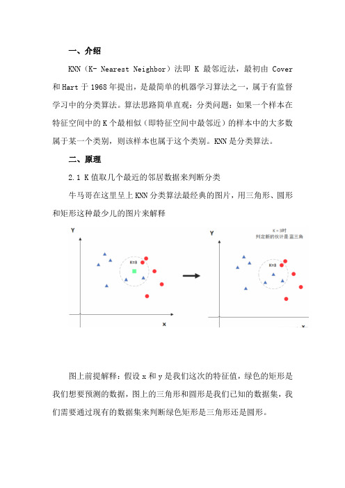
二、原理2.1 K值取几个最近的邻居数据来判断分类牛马哥在这里呈上KNN分类算法最经典的图片,用三角形、圆形和矩形这种最少儿的图片来解释图上前提解释:假设x和y是我们这次的特征值,绿色的矩形是我们想要预测的数据,图上的三角形和圆形是我们已知的数据集,我们需要通过现有的数据集来判断绿色矩形是三角形还是圆形。
当K = 3,代表选择离绿色矩形最近的三个数据,发现三个数据中三角形比较多,所以矩形被分类为三角形当K = 5,代表选择离绿色矩形最近的三个数据,发现五个数据中圆形最多,所以矩形被分类为圆形所以K值很关键,同时建议k值选取奇数。
2.2 距离问题在上面的原理中还有一个关键问题,就是怎么判断距离是否最近。
在这里采用的是欧式距离计算法:下图是在二维的平面来计算的,可以当作是有两个特征值那如果遇到多特征值的时候,KNN算法也是用欧式距离,公式如下:从这里就能看出KNN的问题了,需要大量的存储空间来存放数据,在高维度(很多特征值输入)使用距离的度量算法,电脑得炸哈哈,就是极其影响性能(维数灾难)。
而且如果要预测的样本数据偏离,会导致分类失败。
优点也是有的,如数据没有假设,准确度高,对异常点不敏感;理论成熟,思想简单。
三.KNN特点KNN是一种非参的,惰性的算法模型。
什么是非参,什么是惰性呢?非参的意思并不是说这个算法不需要参数,而是意味着这个模型不会对数据做出任何的假设,与之相对的是线性回归(我们总会假设线性回归是一条直线)。
也就是说KNN建立的模型结构是根据数据来决定的,这也比较符合现实的情况,毕竟在现实中的情况往往与理论上的假设是不相符的。
人工智能技术常用算法

人工智能技术常用算法
一、机器学习算法
1、数据类:
(1)K最近邻算法(KNN):KNN算法是机器学习里最简单的分类算法,它将每个样本都当作一个特征,基于空间原理,计算样本与样本之间的距离,从而进行分类。
(2)朴素贝叶斯算法(Naive Bayes):朴素贝叶斯算法是依据贝叶斯定理以及特征条件独立假设来计算各类别概率的,是一种贝叶斯决策理论的经典算法。
(3)决策树(Decision Tree):决策树是一种基于条件概率知识的分类和回归模型,用通俗的话来讲,就是基于给定的数据,通过计算出最优的属性,构建一棵树,从而做出判断的过程。
2、聚类算法:
(1)K-means:K-means算法是机器学习里最经典的聚类算法,它会将相似的样本分到一起,从而实现聚类的目的。
(2)层次聚类(Hierarchical clustering):层次聚类是一种使用组织树(层次结构)来表示数据集和类之间关系的聚类算法。
(3)谱系聚类(Spectral clustering):谱系聚类算法是指,以频谱图(spectral graph)来表示数据点之间的相互关系,然后将数据点聚类的算法。
三、深度学习算法
1、卷积神经网络(Convolutional Neural Network):卷积神经网络是一种深度学习算法。
knn算法的例子
knn算法的例子k-最近邻算法(k-nearest neighbors,简称k-NN)是一种常用的分类和回归算法。
它基于一个简单的假设:如果一个样本的k个最近邻属于某个类别,那么该样本也很可能属于该类别。
k-NN算法非常直观和易于理解,因此被广泛应用于各种领域。
下面将以几个具体的例子来说明k-NN算法的应用。
1. 手写数字识别在机器学习领域,手写数字识别是一个经典的问题。
k-NN算法可以用于将手写数字图片分类成0到9之间的数字。
基于已有的数字图片数据集,可以计算待分类图片与每个已有图片的距离,并找出k 个最近邻。
然后根据这k个最近邻的标签来判断待分类图片的数字。
2. 电影推荐系统在电影推荐系统中,k-NN算法可以根据用户的历史评分和其他用户的评分来预测用户可能喜欢的电影。
通过计算待推荐电影与用户历史评分电影的相似度,找出k个最相似的电影,并根据这些电影的评分来预测用户对待推荐电影的评分。
3. 股票市场预测k-NN算法可以用于预测股票市场的趋势。
基于已有的股票数据,可以计算待预测股票与历史股票的相似度,并找出k个最相似的股票。
然后根据这k个股票的涨跌情况来预测待预测股票的涨跌。
4. 医学诊断在医学诊断中,k-NN算法可以帮助医生根据患者的各项指标来预测患有哪种疾病。
通过计算待预测患者与已有患者的相似度,找出k 个最相似的患者,并根据这些患者的疾病情况来预测待预测患者的疾病。
5. 文本分类k-NN算法可以用于文本分类,例如将新闻文章分类成不同的主题。
基于已有的训练数据,可以计算待分类文本与每个已有文本的相似度,并找出k个最相似的文本。
然后根据这k个文本的主题来预测待分类文本的主题。
6. 信用评估在信用评估中,k-NN算法可以用于预测申请贷款的人是否具有良好的信用记录。
通过计算待评估人员与已有人员的相似度,找出k个最相似的人员,并根据这些人员的信用记录来预测待评估人员的信用状况。
7. 图像处理k-NN算法可以用于图像处理,例如图像分类和图像检索。
十大经典预测算法
⼗⼤经典预测算法1. 线性回归在统计学和机器学习领域,线性回归可能是最⼴为⼈知也最易理解的算法之⼀。
预测建模主要关注的是在牺牲可解释性的情况下,尽可能最⼩化模型误差或做出最准确的预测。
我们将借鉴、重⽤来⾃许多其它领域的算法(包括统计学)来实现这些⽬标。
线性回归模型被表⽰为⼀个⽅程式,它为输⼊变量找到特定的权重(即系数 B),进⽽描述⼀条最佳拟合了输⼊变量(x)和输出变量(y)之间关系的直线。
线性回归例如:y = B0 + B1 * x我们将在给定输⼊值 x 的条件下预测 y,线性回归学习算法的⽬的是找到系数 B0 和 B1 的值。
我们可以使⽤不同的技术来从数据中学习线性回归模型,例如普通最⼩⼆乘法的线性代数解和梯度下降优化。
线性回归⼤约有 200 多年的历史,并已被⼴泛地研究。
在使⽤此类技术时,有⼀些很好的经验规则:我们可以删除⾮常类似(相关)的变量,并尽可能移除数据中的噪声。
线性回归是⼀种运算速度很快的简单技术,也是⼀种适合初学者尝试的经典算法。
2. Logistic 回归Logistic 回归是机器学习从统计学领域借鉴过来的另⼀种技术。
它是⼆分类问题的⾸选⽅法。
像线性回归⼀样,Logistic 回归的⽬的也是找到每个输⼊变量的权重系数值。
但不同的是,Logistic 回归的输出预测结果是通过⼀个叫作「logistic 函数」的⾮线性函数变换⽽来的。
logistic 函数的形状看起来像⼀个⼤的「S」,它会把任何值转换⾄ 0-1 的区间内。
这⼗分有⽤,因为我们可以把⼀个规则应⽤于 logistic 函数的输出,从⽽得到 0-1 区间内的捕捉值(例如,将阈值设置为 0.5,则如果函数值⼩于 0.5,则输出值为 1),并预测类别的值。
Logistic 回归由于模型的学习⽅式,Logistic 回归的预测结果也可以⽤作给定数据实例属于类 0 或类 1 的概率。
这对于需要为预测结果提供更多理论依据的问题⾮常有⽤。
knn算法的用法
knn算法的用法一、引言K近邻算法(K-NearestNeighbors,简称KNN)是一种基于实例的学习算法,它广泛用于分类和回归问题。
KNN算法以其简单、直观且易于理解的特点,在许多领域得到了广泛应用。
本文将详细介绍KNN算法的原理、应用场景、参数设置以及优缺点,帮助读者更好地理解和应用该算法。
二、KNN算法原理KNN算法的基本思想是通过比较待分类项与已知样本集中的每个样本的距离,找出与待分类项距离最近的K个样本。
根据这K个样本的类别,对待分类项进行预测。
最终,待分类项的类别是由这K个样本中最常见的类别决定。
三、KNN算法的应用场景KNN算法适用于以下场景:1.分类问题:KNN算法可以应用于各种分类问题,如文本分类、图像分类、生物信息学中的基因分类等。
2.回归问题:KNN算法也可以应用于回归问题,如房价预测、股票价格预测等。
3.异常检测:通过比较待分类项与已知样本集的距离,KNN算法可以用于异常检测,识别出与正常样本显著不同的数据点。
四、KNN算法参数设置KNN算法的参数包括:1.K值:确定近邻数,影响算法的准确度和计算复杂度。
过小的K 值可能会导致漏检,而过大的K值可能会导致误检。
需要根据实际问题进行尝试和调整。
2.距离度量方法:KNN算法支持多种距离度量方法,如欧氏距离、曼哈顿距离等。
选择合适的距离度量方法对于算法的性能至关重要。
3.权重策略:在计算待分类项的近邻时,不同的样本可能具有不同的权重。
常见的权重策略包括按照样本出现次数加权、按照距离加权等。
合适的权重策略可以提高算法的准确度和鲁棒性。
五、KNN算法优缺点优点:1.简单易实现:KNN算法实现简单,易于理解和应用。
2.对异常值和噪声具有鲁棒性:KNN算法对异常值和噪声具有较强的鲁棒性,可以有效地处理这些问题。
3.无需大量的参数调优:与其他机器学习算法相比,KNN算法的参数较少,无需进行复杂的参数调优。
缺点:1.对大数据处理能力有限:KNN算法的计算复杂度较高,尤其是在大规模数据集上,处理速度较慢。
knn算法原理
knn算法原理KNN(K近邻算法)是一种基于实例的机器学习算法,是机器学习领域中非常常见的算法。
KNN法的基本思想是:如果一个样本在特征空间中的k个最相近的样本中的大多数属于某一个类别,则该样本也属于该类别。
KNN法中,所选择的邻居都是已经正确分类的对象。
KNN法的基本原理是:在给定一个未知类别的对象(样本数据)时,根据其特征属性和它最接近的K个已经知道分类的样本,对这个对象进行分类。
KNN法就是从训练集中找出这K个“邻居”,根据这K 个“邻居”的类别,来确定当前未知类别的对象的分类。
KNN法的基本流程如下:1. 从训练集中计算测试实例与每个训练集实例之间的距离;2.据距离选择K个最近邻;3.据K个邻居的类别,通过投票或者加权求和,确定测试实例的类别。
KNN法使用数据中“靠近”的训练实例来预测未知实例,因此,KNN法是一种基于实例的学习算法。
KNN法的实质是在训练集中查找与当前输入实例最在的 K 个实例,并将它们的“类标记”作为对应的输入实例的预测。
KNN法的优点是:1. KNN法的思想简单,实现容易,它不需要学习过程,也不需要假设数据的分布,只需要保存所有数据实例;2.实际数据建模时,可以有效地处理属性间关系比较复杂和数据不平衡的情况;3. KNN法可以灵活地处理不同的数据类型。
KNN法也存在一些缺点:1. KNN法需要大量的计算,当训练数据集特别大的时候,搜索K 个最近邻计算量就比较大,可能会耗费较多的时间;2. KNN法的效果依赖于k的值,但是k的值没有一个理论上的确定方法,只能选取不同的k值进行实验;3. KNN法不能很好地处理类别不平衡问题,因为它采用的算法是加权求和,类别不平衡的情况下,加权求和会倾向于那些比较多的类别;4. KNN法的思想是当前的数据点的类别取决于它的K个邻居,而这里的K个邻居都是已经被正确分类的,即每个邻居都是“正确”的,这种认为是不合理的,因为它假定K个邻居的类别都被正确分类了,而这并不一定是真的。
KNN算法原理与应用
12
KNN算法的sklearn实现
sklearn.neighbors模块集成了 k-近邻相关的类,KNeighborsClassifier用做kNN分类
树,KNeighborsRegressor用做kNN回归树。KNeighborsClassifier类的实现原型如下:
class sklearn.neighbors.KNeighborsClassifier(n_neighbors=5, weights='uniform',
testData = [0.2, 0.1]
Result = classify(testData, group, labels, 3)
print(Result)
5
KNN算法基本原理
6
• 运行效果:
•
左下角两个点属于B类用蓝色点标识,右上角
两个点属于A类用红色标识。取k值为3时通过
kNN算法计算,距离测试点(0.2, 0.1)最近的
algorithm='auto', leaf_size=30, p=2, metric='minkowski', metric_params=None, n_jobs=1,
**kwargs)
13
KNN算法的sklearn实现
主要参数如下:
•
•
n_neighbors:整型,默认参数值为5。邻居数k值。
量的kNN搜索。
,适合于样本数量远大于特征数
KNN算法基本原理:距离计算
7
在KNN算法中,如何计算样本间距离非常重要,下面我们介绍几种常见的
距离计算方法。
闵可夫斯基距离
闵可夫斯基距离(Minkowski Distance)是一种常见的方法,用于衡量数值点之间距离。
- 1、下载文档前请自行甄别文档内容的完整性,平台不提供额外的编辑、内容补充、找答案等附加服务。
- 2、"仅部分预览"的文档,不可在线预览部分如存在完整性等问题,可反馈申请退款(可完整预览的文档不适用该条件!)。
- 3、如文档侵犯您的权益,请联系客服反馈,我们会尽快为您处理(人工客服工作时间:9:00-18:30)。
Chapter8k NN:k-Nearest NeighborsMichael Steinbach and Pang-Ning TanContents8.1Introduction (1518.2Description of the Algorithm (1528.2.1High-Level Description (1528.2.2Issues (1538.2.3Software Implementations (1558.3Examples (1558.4Advanced Topics (1578.5Exercises (158Acknowledgments (159References (1598.1IntroductionOne of the simplest and rather trivial classifiers is the Rote classifier,which memorizes the entire training data and performs classification only if the attributes of the test object exactly match the attributes of one of the training objects.An obvious problem with this approach is that many test records will not be classified because they do notexactly match any of the training records.Another issue arises when two or more training records have the same attributes but different class labels.A more sophisticated approach,k-nearest neighbor(kNNclassification[10,11,21],finds a group of k objects in the training set that are closest to the test object,and bases the assignment of a label on the predominance of a particular class in this neighborhood.This addresses the issue that,in many data sets,it is unlikely that one object will exactly match another,as well as the fact that conflicting information about the class of an object may be provided by the objects closest to it.There are several key elements of this approach:(ithe set of labeled objects to be used for evaluating a test object’s class,1(iia distance or similarity metric that can be used to computeThis need not be the entire training set.151152kNN:k-Nearest Neighborsthe closeness of objects,(iiithe value of k,the number of nearest neighbors,and(iv the method used to determine the class of the target object based on the classes and distances of the k nearest neighbors.In its simplest form,k NN can involve assigning an object the class of its nearest neighbor or of the majority of its nearest neighbors, but a variety of enhancements are possible and are discussed below.More generally,k NN is a special case of instance-based learning[1].This includes case-based reasoning[3],which deals with symbolic data.The k NN approach is also an example of a lazy learning technique,that is,a technique that waits until the query arrives to generalize beyond the training data.Although k NN cl assification is a classification technique that is easy to understand and implement,it performs well in many situations.In particular,a well-known result by Cover and Hart[6]shows that the classification error2of the nearest neighbor rule isbounded above by twice the optimal Bayes error3under certain reasonable assump-tions.Furthermore,the error of the general k NN method asymptotically approaches that of the Bayes error and can be used to approximate it.Also,because of its simplicity,k NN is easy to modify for more complicated classifi-cation problems.For instance,k NN is particularly well-suited for multimodal classes4 as well as applications in which an object can have many class labels.To illustrate the last point,for the assignment of functions to genes based on microarray expressionprofiles,some researchers found that k NN outperformed a support vector machine (SVMapproach,which is a much more sophisticated classification scheme[17]. The remainder of this chapter describes the basic k NN algorithm,including vari-ous issues that affect both classification and computational performance.Pointers are given to implementations of k NN,and examples of using the Weka machine learn-ing package to perform nearest neighbor classification are also provided.Advanced techn iques are discussed briefly and this chapter concludes with a few exercises. 8.2Description of the Algorithm8.2.1High-Level DescriptionAlgorithm8.1provides a high-level summary of the nearest-neighbor classification method.Given a training set D and a test object z,which is a vector of attribute values and has an unknown class label,the algorithm computes the distance(or similarity2The classification error of a classifier is the percentage of instances it incorrectly classifies.3The Bayes error is the classification error of a Bayes classifier,that is,a classifier that knows the underlying probability distribution of the data with respect to class,and assigns each data point to the class with the highest probability density for that point.For more detail,see[9].4With multimodal classes,objects of a particular class label are concentrated in several distinct areas of the data space,not just one.In statistical terms,the probability density function for the class does not have a single“bump”like a Gaussian,but rath er,has a number of peaks.8.2Description of the Algorithm 153Algorithm 8.1Basic k NN AlgorithmInput :D ,the set of training objects,the test object,z ,which is a vector ofattribute values,and L ,the set of classes used to label the objectsOutput :c z ∈L ,the class of z foreach object y ∈D do|Compute d (z ,y ,the distance between z and y ;endSelect N ⊆D ,the set (neighborhoodof k closest training objects for z ;c z =argmax v ∈Ly ∈N I (v =class (c y ;where I (·is an indicator function that returns the value 1if its argument is true and 0otherwise.between z and all the training objects to determine its nearest-neighbor list.It then assigns a class to z by taking the class of the majority of neighboring objects.Ties are broken in an unspecified manner,for example,randomly or by taking the most frequent class in the training set.The storage complexity of the algorithm is O (n ,where n is the number of training objects.The time complexity is also O (n ,since the distance needs to be computed between the target and each training object.However,there is no time taken for the construction of the classification model,for example,a decision tree or sepa-rating hyperplane.Thus,k NN is different from most other classification techniques which have moderately to quite expensive model-building stages,but very inexpensive O (constant classification steps.8.2.2IssuesThere are several key issues that affect the performance of k NN.One is the choice of k .This is illustrated in Figure 8.1,which shows an unlabeled test object,x ,and training objects that belong to either a “+”or “−”class.If k is too small,then the result can be sensitive to noise points.On the other hand,if k is too large,then the neighborhood may include too many points from other classes.An estimate of the best value for k can be obtained by cross-validation.However,it is important to point out that k =1may be able to perform other values of k ,particularly for small data sets,including those typically used in research or for class exercises.However,given enough samples,larger values of k are more resistant to noise.Another issue is the approach to combining the class labels.The simplest method is to take a majority vote,but this can be a problem if the nearest neighbors vary widely in their distance and the closer neighbors more reliably indicate the class of the object.A more sophisticated approach,which is usually much less sensitive to the choice ofk ,weights each object’s vote by its distance.Various choices are possible;for example,the weight factor is often taken to be the reciprocal of the squared distance:w i =1/d (y ,z 2.This amounts to replacing the last step of Algorithm 8.1with the154kNN:k-Nearest Neighbors ++‒‒‒‒‒‒‒‒‒‒‒‒‒‒‒‒‒‒‒‒+++X ++++++‒‒‒‒‒‒‒‒‒‒‒‒‒‒‒‒‒‒‒‒‒+++++++++++X ‒‒‒‒‒‒‒‒‒‒‒‒‒‒‒‒‒‒‒‒‒+++++++++++X (a Neighborhood toosmall.(b Neighborhood just right.(c Neighborhood too large.Figure 8.1k -nearest neighbor classification with small,medium,and largek .following:Distance-Weighted V oting:c z =argmax v ∈L y ∈N w i ×I (v =class (c y (8.1The choice of the distance measure is another importantmonly,Euclidean or Manhattan distance measures are used [21].For two points,x and y ,with n attributes,these distances are given by the following formulas:d (x ,y = n k =1(x k −y k 2Euclidean distance (8.2d (x ,y = n k =1|x k −y k |Manhattan distance (8.3where x k and y k are the k th attributes (componentsof x and y ,respectively.Although these and various other measures can be used to compute the distance between two points,conceptually,the most desirable distance measure iswhich a smaller distance between two objects implies a greater likelihood the same class.Thus,for example,if k NN is being applied to classify it may be better to use the cosine measure rather than Euclidean distance.k NN can also be used for data with categorical or mixed categorical and numerical attributes as long as a suitable distance measure can be defined [21].Some distance measures can also be affected by the high dimensionality of the data.In particular,it is well known that the Euclidean distance measure becomes less discriminating as the number of attributes increases.Also,attributes may have to be scaled to prevent distance measures from being dominated by one of the attributes.For example,consider a data set where the height of a person varies from 1.5to 1.8m,8.3Examples155 the weight of a person varies from90to300lb,and the income of a person varies from$10,000to$1,000,000.If a distance measure is used without scaling,the income attribute will dominate the computation of distance,and thus the assignment of class labels.8.2.3Software ImplementationsAlgorithm8.1is easy to implement in almost any programming language.However, this section contains a short guide to some readily available implementations of this algorithm and its variants for those who would rather use an existing implementation. One of the most readily available k NN implementations can be found in Weka[26]. The main function of interest is IBk,which is basically Algorithm8.1.However,IBk also allows you to specify a couple of choices of distance weighting and the option to determine a value of k by using cross-validation.Another popular nearest neighbor implementation is PEBLS(Parallel Exemplar-Based Learning System[5,19]from the CMU Artificial Intelligence repository[20]. According to the site,“PEBLS(Parallel Exemplar-Based Learning Systemis a nearest-neighbor learning system designed for applications where the instances have symbolic feature values.”8.3ExamplesIn this section we provide a couple of examples of the use of k NN.For these examples, we will use the Weka package described in the previoussection.Specifically,we used Weka3.5.6.To begin,we applied k NN to the Iris data set that is available from the UCI Machine Lear ning Repository[2]and is also available as a sample datafile with Weka.This data set consists of150flowers split equally among three Iris species:Setosa,Versicolor, and Virginica.Eachflower is characterized by four measurements:petal length,petalwidth,sepal length,and sepal width.The Iris data set was classified using the IB1algorithm,which corresponds to the IBk algorithm with k=1.In other words,the algorithm looks at the closest neighbor, as computed using Euclidean distance from Equation8.2.The results are quite good, as the reader can see by examining the confusion matrix5given in Table8.1. However,further investigation shows that this is a quite easy data set to classify since the different species are relatively well separated in the data space.To illustrate, we show a plot of the data with respect to petal length and petal width in Figure8.2. There is some mixing between the Versicolor and Virginica species with respect to 5A confusion matrix tabulates how the actual classes of various data instances(rowscompare to their predictedclasses(columns.156kNN:k-Nearest NeighborsTABLE 8.1Confusion Matrix for Weka k NNClassifier IB1on the Iris Data SetActual/Predicted Setosa Versicolor Virginica Setosa5000Versicolor0473Virginica 0446their petal lengths and widths,but otherwise the species are well separated.Since the other two variables,sepal width and sepal length,add little if any discriminating information,the performance seen with basic k NN approach is about the best that can be achieved with a k NN approach or,indeed,any other approach.The second example uses the ionosphere data set from UCI.The data objects in this data set are radar signals sent into the ionosphere and the class value indicates whether or not the signal returned information on the structure of the ionosphere.There are34attributes that describe the signal and 1class attribute.The IB1algorithm applied on the original data set gives an accuracy of 86.3%evaluated via tenfold cross-validation,while the same algorithm applied to the first nine attributes gives an accuracy of 89.4%.In other words,using fewer attributes gives better results.The confusion matrices are given ing cross-validation to select the number of nearest neighbors gives an accuracy of 90.8%with two nearest neighbors.The confusion matrices for these cases are given below in Tables 8.2,8.3,and 8.4,respectively.Adding weighting for nearest neighbors actually results in a modest drop in accuracy.The biggest improvement is due to reducing the number of attributes.P e t a l w i d t h Petal lengthFigure 8.2Plot of Iris data using petal length and width.8.4Advanced Topics157TABLE8.2Confusion Matrix for Weka k NN ClassifierIB1on the Ionosphere Data Set Using All AttributesActual/Predicted Good Signal Bad SignalGood Signal8541Bad Signal72188.4Advanced TopicsTo address issues related to the distance function,a number of schemes have been developed that try to compute the weights of each individual attribute or in some other way determine a more effective distance metric based upon a training set[13,15]. In addition,weights can be assigned to the training objects themselves.This can give more weight to highly reliable training objects,while reducing the impact of unreliable objects.The PEBLS system by Cost and Salzberg[5]is a well-known example of such an approach.As mentioned,k NN classifiers are lazy learners,that is,models are not built explic-itly unlike eager learners(e.g.,decision trees,SVM,etc..Thus,building the model is cheap,but classifying unknown objects is relatively expensive since it requires the computation of the k-nearest neighbors of the object to be labeled.This,in general, requires computing the distance of the unlabeled object to all the objects in the la-beled set,which can be expensive particularly for large training sets.A number of techniques,e.g.,multidimensional access methods[12]or fast approximate similar-ity search[16],have been developed for efficient computation of k-nearest neighbor distance that make use of the structure in the data to avoid having to compute distance to allobjects in the training set.These techniques,which are particularly applicable for low dimensional data,can help reduce the computational cost without affecting classification accuracy.The Weka package provides a choice of some of the multi-dimensional access methods in its IBk routine.(See Exercise4.Although the basic k NN algorithm and some of its variations,such as weighted k NN and assigning weights to objects,are relatively well known,some of the more advanced techniques for k NN are much less known.For example,it is typically possible to eliminate many of the stored data objects,but still retain the classification accuracy of the k NN classifier.This is known as“condensing”and can greatly speed up theclassification o f new objects[14].In addition,data objects can be removed toTABLE8.3Confusion Matrix for Weka k NN ClassifierIB1on the Ionosphere Data Set Using the First Nine AttributesActual/Predicted Good Signal Bad SignalGood Signal10026Bad Signal11214158kNN:k-Nearest NeighborsTABLE8.4Confusion Matrix for Weka k NNClassifier IBk on the Ionosphere Data Set Usingthe First Nine Attributes with k=2Actual/Predicted Good Signal Bad SignalGood Signal1039Bad Signal23216improve classification accuracy,a process known as“editing”[25].There has also been a considerable amount of work on the application of proximity graphs(nearest neighbor graphs,minimum spanning trees,relative neighborhood graphs,Delaunay triangulations,and Gabriel graphsto the k NN problem.Recent papers by Toussaint [22–24],which emphasize a proximity graph viewpoint,provide an overview of work addressing these three areas and indicate some remaining open problems.Other important resources include the collection of papers by Dasarathy[7]and the book by Devroye,Gyorfi,and Lugosi[8].Also,a fuzzy approach to k NN can be found in the work of Bezdek[4].Finally,an extensive bibliography on this subject is also available online as part of the Annotated Computer Vision Bibliography[18].8.5Exercises1.Download the Weka machine learning package from the Weka project home-page and the Iris and ionosphere data sets from the UCI Machine Learning Repository.Repeat the analyses performed in this chapter.2.Prove that the error of the nearest neighbor rule is bounded above by twice theBayes error under certain reasonable assumptions.3.Prove that the error of the general k NN method asymptotically approaches thatof the Bayes error and can be used to approximate it.4.Various spatial or multidimensional access methods can be used to speed upthe nearest neighbor computation.For the k-d tree,which is one such method, estimate how much the saving would ment:The IBk Weka classification algorithm allows you to specify the method offinding nearest neighbors.Try this on on e of the larger UCI data sets,for example,predicting sex on the abalone data set.5.Consider the one-dimensional data set shown in Table8.5.TABLE8.5Data Set for Exercise5x 1.5 2.5 3.5 4.5 5.0 5.5 5.75 6.57.510.5y++−−−++−++References159(aGiven the data points listed in Table8.5,compute the class of x=5.5according to its1-,3-,6-,and9-nearest neighbors(using majority vote.(bRepeat the previous exercise,but use the weighted version of k NN givenin Equation(8.1.ment on the use of k NN when documents are compared with the cosinemeasure,which is a measure of similarity,not distance.7.Discuss kernel density estimation and its relationship to k NN.8.Given an end user who desires not only a classification of unknown cases,butalso an understanding of w hy cases were classified the way they were,which classification method would you prefer:decision tree or k NN?9.Sampling can be used to reduce the number of data points in many kinds ofdata ment on the use of sampling for k NN.10.Discuss how k NN could be used to perform classification when each class canhave multiple labels and/or classes are organized in a hierarchy.AcknowledgmentsThis work was supported by NSF Grant CNS-0551551,NSF ITR Grant ACI-0325949, NSF Grant IIS-0308264,and NSF Grant IIS-0713227.Access to computing facil-ities was provided by the University of Minnesota Digital Technology Center and Supercomputing Institute.References[1] D.W.Aha,D.Kibler,and M.K.Albert.Instance-based learning algorithms.Mach.Learn.,6(1:37–66,January1991.[2] A.Asuncion and D.Newman.UCI Machine Learning Repository,2007.[3] B.Bartsch-Sp¨o rl,M.Lenz,and A.H¨u bner.Case-based reasoning—surveyand future directions.In F.Puppe,editor,XPS-99:Knowledge-Based Systems—Survey and Future Directions,5th Biannual German Conference on Knowledge-Based Systems,volume1570of Lecture Notes in Computer Sci-ence,W¨urzburg,Germany,March3-51999.Springer.[4]J.C.Bezdek,S.K.Chuah,and D.Leep.Generalized k-nearest neighbor rules.Fuzzy Sets Syst.,18(3:237–256,1986.[5]S.Cost and S.Salzberg.A weighted nearest neighbor algorithm for learningwith symbolic features.Mach.Learn.,10(1:57–78,1993.160kNN:k-Nearest Neighbors[6]T.Cover and P.Hart.Nearest neighbor pattern classification.IEEE Transactionson Information Theory,13(1:21–27,January1967.[7] B.Dasarathy.Nearest Neighbor(NNNorms:NN Pattern Classification Tech-puter Society Press,1991.[8]L.Devroye,L.Gyorfi,and G.Lugosi.A Probabilistic Theory of Pattern Recog-nition.Springer-Verlag,1996.[9]R.O.Duda,P.E.Hart,and D.G.S tork.Pattern Classification(2nd Edition.Wiley-Interscience,November2000.[10] E.Fix and J.J.Hodges.Discriminatory analysis:Non-parametric discrimi-nation:Consistency properties.Technical report,USAF School of Aviation Medicine,1951.[11] E.Fix and J.J.Hodges.Discriminatory analysis:Non-parametric discrimina-tion:Small sample performance.Technical report,USAF School of Aviation Medicine,1952.[12]V.Gaede and O.G¨u nther.Multidimensional access methods.ACM Comput.Surv.,30(2:170–231,1998.[13] E.-H.Han,G.Karypis,and V.Kumar.Text categorization using weight adjustedk-nearest neighbor classification.In PAKDD’01:Proceedings of the5th Pacific-Asia Conference on Knowledge Discovery and Data Mining,pages53–65,London,UK,2001.Springer-Verlag.[14]P.Hart.The condensed nearest neighbor rule.IEEE rm.,14(5:515–516,May1968.[15]T.Hastie and R.Tibshirani.Discriminant adaptive nearest neighbor classifica-tion.IEEE Trans.Pattern Anal.Mach.Intell.,18(6:607–616,1996.[16]M.E.Houle and J.Sakuma.Fast approximate similarity search in extremelyhigh-dimensional data sets.In ICDE’05:Proceedings of the21st Interna-tional Conference on Data Engineering,pages619–630,Washington,DC, 2005.IEEE Computer Society.[17]M.Kuramochi and G.Karypis.Gene classification using expression profiles:A feasibility study.In BIBE’01:Proceedings of the2nd IEEE InternationalSymposium on Bioinformatics and Bioengineering,page191,Washington,DC, 2001.IEEE Computer Society.[18]K.Price.Nearest neighbor classification bibliography.http://www.visionbib.com/bibliography/pattern621.html,2008.Part of the Annotated Computer Vision Bibliography.[19]J.Rachlin,S.Kasif,S.Salzberg,and D.W.Aha.Towards a better understandingof memory-based reasoning systems.In International Conference on Machine Learning,pages242–250,1994.References 161 [20] S. Salzberg. PEBLS: Parallel exemplar-based learning system. http://www. /afs/cs/project/ai-repository/ai/areas/learning/systems/pebls/0.html, 1994. [21] P.-N. Tan, M. Steinbach, and V. Kumar. Introduction to Data Minining. Pearson Addison-Wesley, 2006. [22] G. T. Toussaint. Proximity graphs for nearest neighbor decision rules: Recent progress. In Interface-2002, 34th Symposium on Computing and Statistics, Montreal, Canada, April17–20, 2002. [23] G. T. Toussaint. Open problems in geometric methods for instance-based learning. In Discrete and Computational Geometry, volume 2866 of Lecture Notes in Computer Science, pages 273–283, December 6–9, 2003. [24] G. T. Toussaint. Geometric proximity graphs for improving nearest neighbor methods in instance-based learning and data mining. Int. J. Comput. Geometry Appl., 15(2:101–150, 2005. [25] D. Wilson. Asymptotic properties of nearest neighbor rules using edited data. IEEE Trans. Syst., Man, and Cybernetics, 2:408–421, 1972. [26] I. H. Witten and E. Frank. Data Mining: Practical Machine Learning Tools and Techniques, Second Edition (Morgan Kaufmann Series in Data Management Systems. Morgan Kaufmann, June 2005. © 2009 by Taylor & Francis Group, LLC。