Simultaneous Measurement of Non-Commuting Observables
仪器分析常见术语英汉对照
仪器分析常见术语英汉对照Chapter 1 Preface/绪论analytical chemistry/chemical analysis/ instrumental analysis/分析化学/化学分析/仪器分析spectral analysis/光谱分析 electroanalytical chemistry/电分析化学chromatography/色谱法 methods for inorganic species/ 无机物的分析 methods for organic and biochemical species/有机物、生物化学物质的分析description of validation parameters/有效参数的描述precision/精密度 accuracy/准确度 sensitivity/灵敏度 detection limit/检出限quantitation limit/定量限 linearity/线性 linear range/线性范围absolute error/绝对误差 relative error/相对误差 systematic error/系统误差determinate error/可定误差 accidental error/随机误差 indeterminate error/不可定误差debiation/偏差 average debiation/平均偏差 relative average debiation/相对平均偏差 standerd deviation;S/标准偏差(标准差) relatibe standard deviation;RSD/相对平均偏差coefficient of variation/变异系数 propagation of error/误差传递 significant figure/有效数字 partial least squares method ,PLS/偏最小二乘法Chapter 2 Introduction to Optical Methods of Analysis/光学分析导论properties of electromagnetic radiation/电磁辐射的性质 wave properties/波性质 the particle Nature of light: photons/光的粒子性质 interaction of radiation and matter/辐射与物质的相互作用 the electromagnetic spectrum/电磁波谱spectroscopic measurements/光谱测量 radiation absorption/辐射吸收 absorption process/吸收过程 absorption spectra/吸收光谱 limits to Beer's Law/比尔定律的局限性 qualitative sqectrometric analysis/光谱定性分析semiquantitative spectrometric analysis/光谱半定量分析 quantitative spectrometric analysis/光谱定量分析 instruments for optical spectrometry/光谱仪器 spectrophotometer /光谱仪instrument components/仪器的组成部件 optical materials/光学材料 spectroscopic sources/光源 wavelength selectors/单色器 sample containers/样品池spectrophotometer/分光光度计 single beam spectrophotometer/单光束分光光度计double beam spectrophotometer/双光束分子光光度计 dual wavelength spectrophotometer/双波长分光光度计 colorimeter/比色计 visual colorimeter/目视比色计 photoelectric coolorimeter/光电子比色计 holographic grating/全息光栅interference filter/干涉滤光片 calibration filter/校准滤光片 neutral filter/中性滤光片 absorption cell/cuvette/吸收池/比色皿 photocell/photovoltaic cell/光电池photomultiplier/光电倍增管 detecting and measuring radiant energy/辐射能检测signal processors and readouts/信号处理和数据输出molecular Luminescence Analysis/分子发光分析 molecular fluorescence spectroscopy/分子荧光分光光度法 theory of molecular fluorescence/分子荧光光谱法理论 effect of concentration on fluorescence intensity/影响荧光强度的因素 molecular phosphorescence/分子磷光 chemiluminescence methods/化学发光法Chapter 3 Atomic Emission Spectrometry(AES)/原子发射光谱origins of atomic spectra/原子光谱的起源 formation of atomic emission spectra/原子发射光谱的产生 outer electron/外层电子 electron transition/电子跃迁production of atoms and ions/原子和离子的产生 excited potential/激发电位ionization potential/电离电位 transition rule/跃迁定则 energy level diagram/能级图 characteristic spectrum/特征光谱 spectrum line intensity /谱线强度self-absorption and self reversal of spectrum line /谱线的自吸与自蚀 atomization efficiency/原子化效率 atomic line/原子线 resonance line/共振线 sensitive line/灵敏度 Boltzmann distribution/波尔兹曼分布定律 Boltzmann factor/波尔兹曼因子Boltzmann constant/波尔兹曼常数 device and instrument of AES /原子发射光谱分析装置与仪器 types and process of AES /仪器类型与流程 slit/ 狭缝 diffraction grating/衍射光栅 steeloscope/看谱镜 photoelectric direct reading spectrometer/光电直读光谱计 flame photometer/火焰光度计 excitation light source/激发光源 spectrum projictor/映谱仪 spectral photographic plate/光谱感光板microphotometer,microdens-tometer/测微光度计 spectrograph/摄谱仪 plsma source/等离子体[光]源 glow discharge/辉光放电 high firequency discharge/高频放电inductively coupled high frequency plasma torch/电感耦合高频等离子体焰炬capacitively coupled high frequency plasma torch/电容耦合高频等离子体焰炬capacitively coupled microwave plasma torch/电容耦合微波等离子体焰炬 laser microprobe/激光微探针 plate/相板(又称干板) flame spectrometer /火焰光度计 arc and electric spark emission spectrometer/电弧和电火花发射光谱仪 sample introduction systems/样品引入系统 multi-element/多元素 plasma sources/等离子体光源 electrothermal atomizers/电热原子化器 other atomizers/其它原子化器 sources of nonlinearity in atomic emission spectrometry/非线性光源plasma emission spectrometry/等离子发射光谱 direct current plasma jet(DCP)/直流等离子体喷焰 inductively coupled plasma(ICP)/电感耦合等离子体 principle and feature of ICP-AES /电感耦合等离子体发射光谱原理和特点 microwave induced plasma( MIP)/微波感生等离子体 interferences in plasma and flame atomic emission spectroscopy/等离子体和火焰原子光谱中的干扰 matrix interference/基体干扰photomultiplier tube (PMT)/光电倍增管 charge injection detector(CID)/电荷注入式检测器 qualitative and quantitative analysis method /定性和定量分析方法linear dispersion/曲线 angular dispersion/线色散 angular dispersion/角色散reciprocal linear dospersion/倒数线色散 resolving power,resolution/分辨本领spectral line interfernce/谱线干扰 spectral interference/光谱干扰 ionization interference/电离干扰 chemical interference/化学干扰 emission interference/发射干扰 matrix modifier/基体改进剂 spectral buffer/光谱缓冲剂 background absorption/背景吸收 maximum absorption/最大吸收 molecular absorption/分子吸收background absorption Correction/背景吸收校正 enhancement effect/增感效应depression effect/抑制效应Chapter 4 Atomic Absorption Spectrometry and Atomic Fluorescence Spectrometry /原子吸收光谱和原子荧光光谱absorption line/吸收线 resonance line/共振线 line profile/分析线 line profile/谱线轮廓 line width/谱线宽度 entegrated absorption method/积分吸收法 peak absorption method/峰分吸收法 Zeeman effect/塞曼效应 atomization/原子化 line width effects in atomic absorption/原子吸收中的变宽效应 flame atomic absorption/火焰原子吸收 relaxation processes/弛豫过程 atomic absorption with electrothermal atomization/ 原子吸收与电热原子化 interferences in atomic absorption/原子吸收中的干扰 fame atomizers/火焰原子化器 atomic fluorescence spectrometry/原子荧光光谱法 fluorescent species/荧光物质类型 fluorescence instruments/荧光光谱仪applications of fluorescence methods/荧光法的应用Chapter 5 Ultraviolet and Visible Absorption Spectroscopy/紫外-可见吸收光谱ultraviolet-visible absorption spectrometry/紫外可见吸收光谱 ultraviolet-visible photometers and spectrophotometers/紫外—可见分光光度计 spectrophotometric methods/分光光度法 apsorbing species/吸收类型 single-beam Instruments/单光束分光光度计 double-beam instruments/双光束分光光度计 multichannel instruments/多通道仪器 shoulder peak/肩峰 end absorbtion/末端吸收 chromophore/吸收生色团auxochrome/助色团 electron donating group/供电子取代基 electron with-drawing group/吸电子取代基 red shift/红移 blue shift/蓝(紫)移 bathochromic shift/长移hypsochromic shift/短移 hyperchromic effect/增色效应(浓色效应) hypochromic effect/减色效应(淡色效应) strong band/强带 weak band/弱带 absorption band吸收带 transmitance,T/透光率 absorbance/吸光度 band width/谱带宽度 stray light/杂散光 noise/ 噪声 dark noise/暗噪声 signal shot noise/散粒噪声 blazed grating/闪耀光栅 holographic graaing/全息光栅 photodiode array detector/光二极管阵列检测器convolution spectrometry/褶合光谱法 convolution transform,CT/褶合变换 wavelet transform,WT/离散小波变换 multiscale analysis/多尺度细化分析Chapter 6 Infrared Absorption Spectroscopy/红外吸收光谱infrared ray,IR/红外线 mid-infrared absorption spectrum/Mid-IR/中红外吸收光谱far infrared /Far-IR/远红外 near infrared/近红外 microwave spectrum,MV/微波谱infrared spectroscopy/红外吸收光谱法 infrared spectrophotometry/红外分光光度法mode of vibration/振动形式 stretching vibration/伸缩振动 symmetrical stretchingvibration/对称伸缩振动 asymmetrical stretching vibration/不对称伸缩振动 bending vibration/弯曲振动 formation vibration/变形振动 in-plane bending vibration,β/面内弯曲振动 scissoring vibration,δ/剪式振动 rocking vibration,ρ/面内摇摆振动out-of-plane bending vibration,γ/面外弯曲振动 wagging vibration,ω/面外摇摆振动twisting vibration ,τ/蜷曲振动 symmetrical deformation vibration ,δs/对称变形振动 asymmetrical deformation vibration, δas/不对称变形振动 ring prckering vibration/环折叠振动 charateristic avsorption band/特征吸收峰 characteristic frequency/特征频率 correlation absorption band/相关吸收峰 hybridization affect/杂化影响 ring size effect/环大小效应 intensity of absorption band/吸收峰的强度deactivation/去活化过程 vibrational relaxation(VR)/振动弛豫 vibration spectrum/振动光谱 internal Conversion(IC)/内转换 external conversion(EC)/外转换intersystem conversion(ISC)/系间跨跃 dichroism/二色性 wave number calibration/波数校准 group frequency/基团频率 cell-in -cell-ort method/池入-池出法 baseline/基线法 stray light/杂散法 infrared spectrophotometers/红外分光光度计 infrared absorption spectra/红外吸收光谱 absorption intensity/吸收强度 fundamental frequency band/基频谱带 spurious band/乱真谱带 vibrational-rotational spectrum/振转光谱 instruments for infrared spectroscopy/红外光谱仪器fourier transform infrared spect-rometer(FTIR)/傅里叶这换红外光谱计 infrared source/红外光源 infrared beam condenser/红外光束聚光器 infrated polarizer/红外偏振器 studies of complex ions/络合物研究 dispersive infrared instruments/色散型红外光谱仪 fourier transform instruments/傅立叶变换红外光谱仪Chapter 7 Nuclear Magnetic Resonance (NMR) Spectroscopy/核磁共振波谱学introduction to NMR Spectroscopy/核磁谱的简介 definition of NMR Spectroscopy/核磁谱学的定义 NMR History/核磁的历史 properties of nuclei/核的性质 nuclear magnetic resonance,NMR/核磁共振 NMR spectrum/核磁共振波谱 NMR spectroscopy/核磁共振波谱法 continuous wave NMR,CW NMR/连续波核磁共振 fourier transformation NMR spectrum/ FT-NMR/傅立叶变换核磁共振谱 proton magnetic resonance spectrum,PMR/质子核磁共振谱 1H NMR and 13C NMR spectrum/氢谱和碳-13核磁共振谱 spin angular momentum/自旋角动量 magnetogyric ratio/磁旋比 magnetic quantum number,m/磁量子数precession/进动 relaxation mechanism/弛豫历程 local diamagnetic shielding/局部抗磁屏蔽 shielding constant/屏蔽常数 swept field/扫场 seept frequency/扫频schematic NMRspectrometer/核磁仪的概图 magnetic anisotropy/磁各向异性 long range shielding effect/远程屏蔽效应 magnetic eqivalence/磁等价 spin system/自旋系统chemical shift/化学位移 standard for chemical shift/核磁的内标物 shielding and deshielding/屏蔽和去屏蔽效应 spin-spin coupling/自旋-自旋耦合 J-coupling/ J-耦合spin-spin coupling/自旋-自旋偶合 spin=spin splitting/自旋-自旋分裂 coupling constant/耦合常数 decoupling/去耦 nodal plane/结面 factors to affect 1Hchemical shift/影响氢化学位移的因素 signalsplitting for 1H/氢谱的裂分 chemical shift - 13C-NMR/碳谱的化学位移 13C-NMR integration/碳谱中积分 interpreting NMR spectra/核磁谱的解析 2D NMR/二维核磁共振 singlet,s/单峰 doublet,d/双峰 triplet,t/三重峰quartet/ quintet/ sextet/四重峰/五重峰/六重峰 geminal coupling /vicinal coupling/偕偶/邻偶 long range coupling/远程偶合 first order spectrum/一级光谱 second order spectrum/二级光谱(二级图谱) C-H correlated spectroscopy,C-H COSY/C-H光谱Chapter 8 Introduction to Electrochemistry/电化学导论electrochemical analysis/电化学分析 electrolytic analysis method/电解法electtogravimetry/电重量法 coulometry/库仑分析法(电量分析) coulometric titration/库仑滴定法 conductometry/电导法 conductometric analysis/电导分析法conductometric titration/电导滴定法 potentiometry/电位分析法 dirext potentiometry直接电位法 potentiometric titration/电位滴定法 voltammetry/伏安法polarography/极谱法 stripping method/溶出法 amperometric titration/电流滴定法chemical double layer/化学双电层 phase boundary potential/相界电位 electrode potential/金属电极电位 chemical cell/化学电池 liquid junction boundary/液接界面galvanic cell/原电池 electrolytic cell/电解池 cathrode/负极 anode/正极eletromotive force/电池电动势 potentials/电极电势 Plank constant/普朗克常数Nernst equation/能斯特方程 indicator electrode/指示电极 reference electroade/参比电极Chapter 9 Potentiometry/电位法principles of potentiometric measurements/电位法测定原理 direct potentiometry/直接电位法 potentiometric titrations/电位滴定法 standard hydrogen electrode/标准氢电极 primary reference electrode/一级参比电极 standard calomel electrode/饱和甘汞电极 silver silver-chloride electrode/银-氯化银电极 liquid junction boundary/液接界面 asymmetry potential/不对称电位 apparent PH /表观PH值combination PH electrode/复合PH电极 ion selective electrode/离子选择电极 sensor/敏感器 crystalline electrodes/晶体电极 homogeneous membrance electrodes/均相膜电极 heterog eneous membrance electrodes/非均相膜电极 non- crystalline electrodes/非晶体电极 rigid matrix electrode/刚性基质电极 electrode with a mobile carrier/流流体载动电极 gas sensing electrodes/气敏电极 enzyme electrodes/酶电极 glass electrodes/玻璃电极 liquid membrane electrodes/液膜电极 solid-state electrodes/固体电极 selectivity coefficient/选择性系数 electrode-ealibration method/电极校正方法 standard-addition method/标准加入法Chapter 10 Electrolytical Analysis and Coulometry/电解分析法和库仑法bulk electrolysis: electrogravimetry and coulometry/整体电解:电重量法和库仑法controlled-Current electrolytical analysis/控制电流电解法 controlled -Potentil electrolytical analysis/控制电势电解法 choice of negative potential/负极电位的选择 controlled-Potential coulometry/控制电势库仑法 coulometric titration/库仑滴定法 coulometric methods/库仑分析法Chapter 11 Voltammetry and Polarograph/伏安法和极谱法polarography/极谱法 polarogram/极谱图 polarography Equation/极谱波方程linear-sweep Voltammetry /线性扫描伏安法 cyclic voltammetry/循环伏安法 pulse polarographic and voltammetri cmethods/脉冲极谱和伏安法 polarography catalytical waves/极谱催化波 parallel polarographic catalytic wave/极谱平行催化波 hydrogen catalytic wave/氢催化波 adsorptive complex wave/络合物吸附波 stripping voltammetriy/溶出伏安法 anodic stripping voltammetry/阳极溶出伏安法 cathodic stripping voltammetry/阴极溶出伏安法Chapter 12 Chromatography: Theory and Concepts/色谱分析法理论与概念concepts and terms/概念及术语 chromatography/色谱法(层析法) chromatography processor/色谱过程 stationary phase/固定相 mobile phase/流动相 peak height/峰高peak width,W/峰宽 peak width at half height,W1/2 or Y1/2/半峰宽leading peak/前延峰 tailing peak/拖尾峰 symmetry factor,fs/对称因子 retention time/保留时间 retention volume/保留体积 dead time/死时间 asjusted retention time/调整保留时间 isotherm line/等温线 height equivalent to atheoretical plate/理论塔板高度分离度resolution normalization method/归一化法 external standardization外标法 distribution cofficient/分配系数 partition coefficient/狭义分配系数 plate theory/塔板理论 number of theoretical plates/理论塔板数 rate theory/theory of rate/速率理论 resolution ,R/分离度 separation number,SN/分离数 relative Rf, Rr/相对比移值 gas chromatography,GC/气相色谱法 liquid cromatography,LC/液相色谱法planar, plane chromatography//平板色谱法 paper chromatography/纸色谱法 thin layer chromatography ,TLC/薄层色谱法thin film chromatography/薄膜色谱法 capillary electrophoresis,CE/毛细管电泳法high-performance/高效 high performance capillary electroporesis,HPEC/高效毛细管电泳法 high performance liquid chromatography,HPLC/高效液相色谱法 normal-phase/正相 recersed-phase/反相 ion-exchange/离子交换 gel-filtration/凝胶过滤chromatography applications database/色谱应用数据库Chapter 13 Gas chromatography/气相色谱法chemically bonded phase/化学键合相 polydiethylene glycol succinate,PDEGS,DEGS/丁二酸二乙二醇聚酯 GDX/高分子多孔微球 STY/苯乙烯; EST/乙基乙烯苯; DVB/二乙烯苯wall coated open tubular column,WCOT/涂壁毛细管柱 supprot coated open tubular column,SCOT/载体涂层毛细管柱 thermal conductivity detector,TCD/热导检测器hydrogen flame ionization detector,FID/氢焰离子化检测器 electron capture detector ,ECD/电子捕获检测器 noise,N/噪声 drift,d/漂移 column chromatography/柱色谱法 column selector/柱子的选择 packed column/填充柱 capillary column/毛细管柱microbore packed column 微填充柱 instruments in gas chromatography/气相色谱仪GC/MS: instruments and applications/气相色谱-质谱联用技术Chapter 14 High performance liquid chromatography/高效液相色谱liquid –solid chromatography adsorption ,LSC/液-固吸附色谱(液固色谱法)liquid-liquid partition chromatography液-液分配色谱法(分配色谱) normal phase,NP/正相 reversed phase, RP/反相 octadecylselyl,ODS/十八烷基 isocraic elution/恒组成溶剂洗脱 gradient elution/梯度洗脱 ion exchange chromatography,IEC/离子交换色谱法 chemically bonde phase/化学键合相 bonded phase chromatography,BPC/键合相色谱法 chemically bonded-phase chromatography/化学键合相色谱法 ion chromatography,IC/离子色谱法 paired ion chromatography,PIC/离子对色谱法 ion suppression chromatography,ISC/离子抑制色谱法 steric exclusion chromatography,SEC/空间排阻色谱法 size-exclusion chromatography/尺寸排阻色谱gel chromatography/凝胶色谱法 gel permeation chromatography,GPC/凝胶渗透色谱法gel filtration chromatography,GFC/凝胶过滤色谱法 permeation coefficien;Kp/渗透系数 chiral chromatography,CC/手性色谱法 chiral stationary phase,CSP/手性固定相cyclodextrin chromatography,CDC/环糊精色谱法 micellar chromatography,MC/胶束色谱法 affinity chromatography,AC/亲和色谱法 supercritical fluid chromatography,SFC/超临界流体色谱法 end capping/封尾、封顶、遮盖 capillary electrophoresis/毛细管电泳 instruments in capillary electrophoresis/毛细管电泳仪 electroosmotic flow/电渗流 criticak micolle concentration ,CMC/临界胶束浓度 DNA sequencing and capillary array electrophoresis/DNA序列分析及毛细管阵列电泳ultraviolet detector,UVD/紫外检测器 fluorophotomeric detector,FD/荧光检测器 ECD/电化学检测器 RID/示差折光检测器 photodiode array detector ,DAD/光电二极管检测器3D-spectrochromatogram/三维光谱-色谱图 evaporative light scatteringdetector,ELSD/蒸发光散射检测器 ampere detector,AD、安培检测器 high performance capillary electrophoresis,HPCE、高效毛细管电泳法 mobility/淌度 electrophoresis/电泳 electroosmosis/电渗 hydrodynamic injection/动力进样 electrokinetic injection/电动进样 capillary zone electrophoresis,CZE/毛细管区带电泳法 micellar electrokinetic capillary chromatography,MECC/胶束电动毛细管色谱 capillary gel electrophoresis,CGE/毛细管凝胶电泳 sieving筛分 thin layer plate/薄层板;TLC/薄层色谱法 adsorption/吸附 activation/活化 deactivation/脱活性 degree of cross linking/交联度 exchange capacity/交换容量 developing solvent ,developer/展开剂Chapter 15 Mass Spectrometry /质谱分析法mass spectrum,MS/质谱 bar graph/棒图 selected ion monitoring ,SIM/选择离子检测direct probe inlet ,DPI/直接进样 interface/接口 gas chromatography-mass spectrometry,GC-MS/气相色谱-质谱联用 high performance liquidchromatography-mass spectrometry,HPLC-MS /高效液相色谱-质谱联用ionizationmethods/离子化方法 electron impact source,EI/电子轰击离子源 fast atom bombardment ,FAB/快速原子轰击离子源 chemical ionization source,CI/化学离子源field ionization,FI/场电离 field desorptiion,FD/场解析 matrix assisted laser desorption (MALDI)/基质辅助的激光解吸 electro spray ionization ( ESI )/电喷雾 mass analyzer/质量分析器 magnetic-sector mass spectrometer/磁质谱仪 quadrupole mass spectrometer/四极杆质谱仪(四极质谱仪)amu/原子质量单位 ion abundance/离子丰度 relative avundance/相对丰度(相对强度) base peak/基峰 mass range/质量范围 resolution/分辨率 sensitivity/灵敏度 S/N /信噪比 molecular ion/分子离子 fragment ion/碎片离子 isotopic ion/同位素离子metastable ion/亚稳离子 metastable peak/亚稳峰 parent ion/母离子 daughter ion/子离子 odd electron/含奇数个电子的离子 even eletron,EE/含偶数个电子的离子homolytic cleavage/均裂 heterolytic cleavage/异裂(非均裂) hemi-homolysis cleavage/半均裂 rearragement/重排 MW/分子量α-cleavage/α-裂解 relative Abundance of Isotopes/同位素的相对丰度 isotopic Ratio from the Spectra/质谱中的同位素比例 magnetic sector analyzer/磁分析器 time of flight analyzer/飞行时间分析器 quadrupole analyzers/四极质量分析器 fourier transform ioncyclotron/傅立叶离子回旋共振分析器 MS interpretation and fragmentation/质谱解析和化合物裂解presentation of data/数据表达 determination of Molecular Mass/分子量的测量 high resolution mass spectrometry/高分辨质谱 important fragmentation patterns in EI/ 电子轰击电离下的重要裂解方式patterns of different organic compounds’ fragmentation/不同类型有机物的裂解模式 hyphenated MS techniques/质谱联用技术。
自控中英对照

Z-transform, Inverse Z Transform z变换, z反变换Stability, Dynamic Performance, Steady-state Errors, 稳定性,动态性能,稳态误差the continuous-time state equation, the continuous-time system (signal)连续状态方程,连续系统(信号)the discrete time state equation, the discrete-time system (signal)离散状态方程,离散系统(信号)initial state of the system 系统的初始状态the solution of this homogeneous (non-homogeneous) state equation齐次(非齐次)状态方程的解the sample time 采样时间the parameters 参数the condition 条件Controllable, controllability 可控的,可控性Observerable, observerablity 可观的,可观性plot the figure 画图obtain the closed-loop impulsive transfer function获得闭环系统的脉冲传递函数determine the stable range of k 判定k的稳定区间nonlinear system非线性系统the describing function of nonlinear part非线性部分的描述函数plot the curves 画出轨迹self-oscillation 自激振荡the input signal 输入信号establish the equations of switching lines and plot the phase portrait of system建立方程的切换线方程,并绘制相轨迹Obtain all singular points and their types获得所有的奇点并判断它们的类型the transfer function of the system 系统的传递函数Controllable and Observable Canonical Form 可控和可观标准型Diagonal Canonical Form 对角线标准型Jordan Canonical Form 约当标准型state space expression 状态空间表达式the State Variables Diagram 状态空间结构图state feedback 状态反馈state observer状态观测器the expected poles of the state feedback system 状态反馈系统的期望极点the expected poles of the designed state observer 设计的状态观测器的期望极点1。
Numerical_and_Experimental_Examination_for_Oil_Pump_System_Using_a_Simplified_Uncoupled_Simulation_a
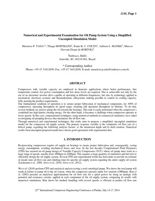
Numerical and Experimental Examination for Oil Pump System Using a SimplifiedUncoupled Simulation ModelMauricio P. TADA1*, Thiago HOFFMANN1, Paulo R. C. COUTO1, Adilson L. MANKE1, MarcosGiovani Dropa de BORTOLI11Embraco, R&D,Joinville, SC, 89219-901, Brazil* Corresponding AuthorPhone: +55 47 33412650, Fax: +55 47 34412650, E-mail: mauricio.p.tada@.brABSTRACTCompressors with variable capacity are employed in domestic applications where better performance, fine temperature control, low power consumption and low noise levels are required. This is achievable not only by the use of an electronic inverter drive capable of operating at different frequencies, but also by technology applied in mechanical, electrical, acoustic and thermodynamic subsystems, making possible to control its cooling capacity, fully meeting the product requirements.One fundamental condition of operation is to ensure proper lubrication of mechanical components, for 100% of compressors, operating throughout its speed range, ensuring full operation throughout its lifetime. To do that, several methods are used to pump the oil towards the bearings. This task is easily performed when the compressor’s crankshaft has high kinetic rotating energy. On the other hand, it becomes a challenge when compressor operates at lower speeds. In this case, computational techniques, using numerical methods in commercial simulators, have aided on designing oil pumping devices that maximizes the oil flow rate.Through numerical and experimental techniques, this study aims to propose a simplified, uncoupled simulation model for the compressor oil supply system. The primary response variable is the volumetric oil flow rate of a helical pump, regarding the following analysis factors: a) the immersion depth and b) shaft rotation. Numerical results from uncoupled proposed model have shown good agreement with experimental data.1. INTRODUCTIONReciprocating compressors require oil supply on bearings to ensure proper lubrication and, consequently, saving energy consumption, avoiding mechanical losses and wear. In the last decades Computational Fluid Dynamics (CFD) has assisted on oil pump design of Variable Capacity Compressors (VCC) where oil pump must work in a large range of speeds, usually from 1000rpm to 4500rpm. This requires a large quantity of simulation and lab tests to efficiently design the oil supply system. Several CFD and experimental works has been done to provide an estimate of steady state oil flow rate and climbing time for specific oil supply system regarding the entire supply oil system (Luckmann et al., 2008; Alves et al., 2010; Alves et al., 2012).Wu et al. (2010) perform CFD and analytical analysis testing a reed centrifugal pump. Wu shows the reed pump will result in failure to pump oil to the oil system, when the compressor operates under low rotation (1000rpm). Kim et al.(2002) presents an analytical approximation for oil flow rate for a spiral groove by using an analogy with potential and resistance circuits, applied in each component of the oil supply system, comparing its results with numerical simulations. Kim shows his method, handling with several speeds, is efficient to predict oil flow ratehaving reasonable agreement with experimental tests. However, for each oil pump design it is necessary to have a respective analytical solution. According to his method, by analytics expressions, is it possible to quantify the influence of all elements on the supply system. More recently, Alves et al.(2010) present analytical and CFD solutions for a helical pump, comparing results with experimental data with good agreement. His simulation of the overall system, performed on a Pentium D-930, takes 336 hours. He also presents a semi-analytical method taking few seconds to predict oil flow rate, with maximum error of order of 12%, however some important simplification on semi-analytical method, mainly on low speed, had been assumed, for example, the gap between pin and sleeve pump not being taken in account.The Present work aims to propose a simple, uncoupled CFD model for reciprocating compressor oil supply system, aiming to predict the oil flow rate efficiently over the lower VCC compressors speed range. Figure 1 shows a typical reciprocating compressor’s oil supply system. The analysis has been performed experimentally on entire system and numerically on component highlighted, called “oil pump” in an uncoupled way, i.e., instead to simulate all oil supply system, the model takes in account only the components 5a and 5b of a helical pump as shown on Figure 1. Experimental verification has been made with lab tests detailed on Section 3. Primary response variable is the volumetric oil flow rate respect to the following analysis factors: a) the immersion depth and; b) shaft rotation. The immersion is eligible for varying the hydrostatic pressure on inlet pump, being a factor for evaluating the proposed numerical boundary condition detailed on Section 2.3.Figure 1: Oil supply system and helical oil pump detail.2. NUMERICAL SIMULATIONMain assumptions on the mathematical model are: a) isothermal; b) constant density and viscosity; c) no interfacial tension; d) laminar flow; e) uncoupled oil pump with respect to oil pump system. The geometry of oil system evaluated is able to pump at low and high speeds, however present work is dedicated to low speeds. Thus by hypothesis it is assumed an “infinite conductivity” in all remaining system, i.e., the shaft channel (8) and eccentric channel (2) resistance is neglected and system performance is defined by oil pump.2.1 Fundamentals of the mathematical modelThe CFD results were obtained by using a laminar, homogeneous, free surface model on Ansys-CFX®. According to Ansys® help system (2013a), the method used to solve fundamental equations are the volume of fluid (VOF)method. A free surface refers to an interface between a gas and a liquid, where the difference in the densities between the two is quite large. Due to the low density, the inertia of the gas is usually negligible, so the only influence of the gas is the pressure takes place at the interface. Hence, the gas region do not need to be modeled, and the free surface is simply modeled as a boundary with constant pressure. The VOF method determines the shape and location of free surface based on the concept of fluid volume fraction χ. In general, the evolution of the free surface is computed either through a VOF advection algorithm or through the following equation:0=∇⋅+∂∂χχu t(1)In the homogeneous model, a common flow field is shared by all fluids and the transported quantities αϕ, except volume fractions, are the same for all phases, that is, ϕϕα= for ααN ≤≤1. The bulk transport equations can be derived by summing the individual phase transport equations over all phases to give a single transport equation for ϕ:()()S t=∇Γ−⋅∇+∂∂ϕϕρρϕu (2)where 0,0,1==Γ=S ϕrecover the mass balance equation and p S −∇==Γ=ϕϕµϕ,,u recover the laminar momentum equation. In addition the homogeneous model uses the following mixtures variables:∑∑∑===Γ=Γ==αααααααααααααχρχρχρN N N 111,,u u .(3)Therefore, the system of equations is made up by primary five variables P w v u ,,, and χ. The governing equations are (1) and (2) resulting on five equations. In the present work, the flow is air-oil and the one of volume fractions can be computed from restriction volume equation oil gas χχ−=1. Details on modeling VOF and homogeneous model can be found on Ansys® help system (2013a). Barbosa et al. (2008) has also provided details about governing equations and VOF solution method.2.3 Domain and boundary conditionsFigure 2 shows the proposed rotating domain at a rate of Ω [rad/s]. The volume domain is where fluid can flow, being the oil pump “solid’s negative”, as illustrated on Figure 1.Figure 2: Helical pump – solutions domain.The center pin – component 5a on Figure 1 – is modeled as a cylindrical wall inside the pump defined as a counter rotating wall having opposite rotation -Ω [rad/s]. The bottom face inlet is defined as an opening with hydrostatic pressure prescribed, i.e., pressure relative to immersion height. The oil volume fraction defined as 1. Discharge side outlet is defined also as an opening with 0Pa prescribed pressure and volume fraction to be calculated considering zero gradients.Similarly the top gas outlet is stated as opening with pressure 0Pa and gas volume fraction equal to 1. All other faces are defined as no slip walls. Interpolation was defined as pure upwind and residual problem convergence is achieved when all conservation equations reaches 1.0e-4 residual. Inlet flow rate and outlet flow rate is monitored and steady state is achieved when the inlet/outlet volume balance is smaller than 1%. Mesh has about one million of elements to capture efficiently high near wall velocity gradients.3. EXPERIMENTAL VERIFICATIONExperimental lab tests were performed to validate the models employed in the simulation. Figure 3 shows the bench test with the following components: 1) compressor kit (crankcase, motor, crankshaft and oil pump); 2) oil colleting tube; 3) graduated cylinder; 4) oil; 5) heater; 6) oil reservoir; 7) thermocouple and; 8) oil pump. Some additional components used on the experiment are not shown in this figure.Figure 3: Oil flow rate bench test.The mechanical kit compressor (1) has its rotating speed controlled by a frequency inverter in such a way is it possible to operate in a wide speed range with around 5rpm uncertainty. The oil pumped by the oil supply system is collected directly to a graduated cylinder – with 1ml of resolution – when measuring is being performed; otherwise oil flow returns to reservoir, both ways transported by colleting tube (2). Immersion pump is controlled by marks on oil pump matching with oil reservoir height.Before measuring, the entire system must be in thermal equilibrium. The thermocouple located in a vicinity of the oil pump registers temperature continuously, with an uncertainty around 1°C, and the heater has an automatic system control that always tries to keep temperature in a given magnitude. All tests were performed at (50 ± 1)°C, once system achieves equilibrium. In this work, it is adopted a simple approximation to calculate the uncertainties, considering only the repeatability of the entire system for each setup test, neglecting all other uncertainties acting on measure system.4. TEST PLANBoth numerical and experimental tests will be performed according to the present plan. As previously stated, the output variable will be the oil flow rate. The input variables are the pump’s immersion and speed rotation. It must be emphasized in present analysis the pump’s height and all other geometric pump’s variable like pitch, channel depth etc. were kept constant. It is not objective of this work to quantify oil flow rate variation with respect to these geometric variables. Results presented here are supposed valid for a generic helical pump, independent of its intrinsic geometric parameters.Non-dimensional rotating speeds, both numerical and experimental, are evaluated with respect to its maximum value. The experimental tests were performed according to Table 1. For each test setup, nine oil flow rate measurements were carried out, calculating average, standard deviation and uncertainties with 90% of confidence interval. The numerical tests were performed according to the variables levels as shown on Table 2. The levels were combined into enhanced centered face central composite Design Of Experiment (DOE), totalizing seventeen deterministic test simulations performed on Ansys-CFX® in order building a response surface with determination coefficient closer to 1.0 and maximum absolute error closer to 0.0. Details about the probabilistic method can be found on reference Ansys® help system (2013b).Table 1: Experimental lab test setup variables. Table 2: Numerical variables levels.Test setup Speed [-]Height [mm]10.5 3.020.511.530.520.04 1.0 3.05 1.011.5Level Speed [-]Height [mm]1.00.5 3.02.0 1.020.0As previously commented, for each setup test, nine measurements were performed and average, standard deviation and uncertainty were calculated considering a Student t-distribution. The “t” value employed was 1.83 once the interval confidence regard is 90%. The uncertainties on dimensional measuring system were neglected for being considered small.5. RESULTS AND DISCUSSIONSAs remarked, experimental lab tests were performed with entire oil supply system and compared with uncoupled simulation oil pump results. Figure 4a shows numerical and experimental oil flow varying with rotating and discharge height. All experimental results overlap each other, showing the minimal influence of immersion pump on oil flow rate. The delimited gray area shown in Figure 4b represents estimatives for experimental uncertainties, with 90% of confidence interval, along rotation and immersion pump range. Numerical results were gathering from a standard response surface – full 2nd order polynomials – with determination coefficient equals to 0.99977 and maximum absolute error equals to 2.45. Table 3 summarizes experimental results and uncertainties calculation. The numerical uncoupled simulation model shows good agreement with experimental results and higher sensibility for immersion pump as discussed below.(a) (b)Figure 4: Oil flow rate over dimensionless rotation and discharge height: (a) experimental and numerical results; b) experimental uncertainties and interval of confidence for oil flow rate varying with rotation and immersion.Perhaps the main reason of the numerical sensitivity to immersion height is relative to boundary condition at both inlet and outlet oil pump region. The outlet neglects any resistance along oil supply system and inlet considers only hydrostatic pressure. Despite relative sensitivity respect to immersion as shown on Figure 2a, numerical curve was achieved with seventeen numerical simulations of oil pump, having grid with around one million of elements and taking about two hours each simulation on Intel Core i7-3720. Taken the need of several simulations when oil supply system is designed for VCC compressors, the proposed uncoupled model may be a good approach to assist on designing the oil pump.Table 3: Summary of experimental results.Test setup Speed [-]Height [mm]Average oil flow[ml/min]Standard deviation[ml/min]Uncertainty[ml/min]10.5 3.031.333 2.500 4.58320.511.531.111 1.042 1.90930.520.032.1110.551 1.0104 1.0 3.069.500 1.875 3.4375 1.011.568.611 1.042 1.9096 1.020.069.2220.908 1.6656. CONCLUSIONSThe Present work evaluated an uncoupled simulation model proposed by varying immersion’s pump height and compressor speed, comparing results with experimental tests. The CFD model did not consider the oil supply system as a whole, but only the oil pump. The following conclusions can be stated:•Simplified uncoupled numerical proposed model shows good agreement with experimental data and efficient computational effort;•Immersion shows minimal effects on experimental oil flow rate and small sensibility on numerical results.NOMENCLATURERomanN number of phase (–)u vector mixture velocity (m/s)N number (–)S 0, minus pressure gradient (–, Pa/m)h dimensionless discharge height (–)Greekχvolume fraction (–)Ωangular velocity (rad/s)ρdensity (kg/m³)φunit, mixture velocity (–, m/s)Γnull, viscosity (–, Pa s)Subscriptαphase oil or gasREFERENCESAlves, M. V. C., Barbosa, J.R. Jr., Prata, A. T., Ribas, F. A. R. Jr., 2010, Fluid Flow in a Screw Pump Oil Supply System for Reciprocating Compressors, Int. Compressor Engineering Conference at Purdue, Paper 1326 Alves, M. V. C., Barbosa, J.R. Jr., Prata, A. T., Analytical and CFD Modeling of the Fluid Flow in an Eccentric-Tube Centrifugal Oil Pump for Hermetic Compressors, Int. Compressor Engineering Conference at Purdue, Paper 1127Ansys®, 2013, Release 14.5, Help System, Mechanical APDL, Fluids Analysis Guide, Theory Reference, Fluid Flow, Ansys, Inc.Ansys®, 2013, Release 14.5, Help System, Mechanical APDL, Fluids Analysis Guide, Theory Reference, Probabilistic Design, Ansys, Inc.Barbosa, J. R.Jr., Lückmann, A. J., Alves, M. V. C., Pizarro-Recabarren, R. A., 2008, Utilização do Método do Volume de Fluido (VOF) na Simulação de Escoamentos Bifásicos com Superfície Livre em Compressores Herméticos, EBECEM – 1°Encontro Brasileiro sobre Ebulição, Condensação e Escoamento MultifásicoLíquido-Gás, Florianópolis, SC, Brazil.Kim, H. J., Lee, T. J., Kim, K. H., and Bae, Y. J., 2002, Numerical Simulation Of Oil Supply System Of Reciprocating Compressor For Household Refrigerators, Int. Compressor Engineering Conference at Purdue, Paper 1533Wu, W., Li, J., Lu, L., Feng, Q., 2010, Analysis of Oil Pumping in the Hermetic Reciprocating Compressor for Household, Int. Compressor Engineering Conference at Purdue, Paper 1168.ACKNOWLEDGEMENTThe present paper authors would like to thank: Embraco’s DSMM/R&D leader Raul Bosco Jr. for his support, revision and incentive; Embraco’s draftsman Emerson Moreira for helping on figures; Emilio Rodrigues Hulse for helping on technical discussions and; Fabian Fagotti for careful revision.。
simultaneous equation method
Simultaneous Equation MethodIntroductionIn mathematics, simultaneous equations play a crucial role in solving real-world problems and modeling various phenomena. The simultaneous equation method is a powerful technique used to find solutions for a system of equations. This method involves solving multiple equations together to determine the values of unknown variables. In this article, we will explore the simultaneous equation method in detail and discuss its applications.Understanding Simultaneous EquationsDefinitionSimultaneous equations, also known as a system of equations, are a set of equations that share the same variables. The solutions of these equations simultaneously satisfy each equation in the system. The general form of simultaneous equations can be written as:a1x + b1y = c1a2x + b2y = c2Here, x and y are the variables, while a1, a2, b1, b2, c1, and c2 are constants.Types of Simultaneous EquationsSimultaneous equations can be classified into three types based on the number of solutions they have:1.Consistent Equations: These equations have a unique solution,meaning there is a specific set of values for the variables thatsatisfy all the equations in the system.2.Inconsistent Equations: This type of system has no solution. Theequations are contradictory and cannot be satisfied simultaneously.3.Dependent Equations: In this case, the system has infinitely manysolutions. The equations are dependent on each other and represent the same line or plane in geometric terms.To solve simultaneous equations, we employ various methods, with the simultaneous equation method being one of the most commonly used techniques.The Simultaneous Equation MethodThe simultaneous equation method involves manipulating and combining the given equations to eliminate one variable at a time. By eliminating one variable, we can reduce the system to a single equation with one variable, making it easier to find the solution.ProcedureThe general procedure for solving simultaneous equations using the simultaneous equation method is as follows:1.Identify the unknow n variables. Let’s assume we have n variables.2.Write down the given equations.3.Choose two equations and eliminate one variable by employingsuitable techniques such as substitution or elimination.4.Repeat step 3 until you have a single equation with one variable.5.Solve the single equation to determine the value of the variable.6.Substitute the found value back into the other equations to obtainthe values of the remaining variables.7.Verify the solution by substituting the found values into all theoriginal equations. The values should satisfy each equation.If the system is inconsistent or dependent, the simultaneous equation method will also lead to appropriate conclusions.Applications of Simultaneous Equation MethodThe simultaneous equation method finds applications in numerous fields, including:EngineeringSimultaneous equations are widely used in engineering to model and solve various problems. Engineers employ this method to determine unknown quantities in electrical circuits, structural analysis, fluid mechanics, and many other fields.EconomicsIn economics, simultaneous equations help analyze the relationship between different economic variables. These equations assist in studying market equilibrium, economic growth, and other economic phenomena.PhysicsSimultaneous equations are a fundamental tool in physics for solving complex problems involving multiple variables. They are used in areas such as classical mechanics, electromagnetism, and quantum mechanics.OptimizationThe simultaneous equation method is utilized in optimization techniques to find the optimal solution of a system subject to certain constraints. This is applicable in operations research, logistics, and resource allocation problems.ConclusionThe simultaneous equation method is an essential mathematical technique for solving systems of equations. By employing this method, we can find the values of unknown variables and understand the relationships between different equations. The applications of this method span across various fields, making it a valuable tool in problem-solving and modeling real-world situations. So, the simultaneous equation method continues to be akey topic in mathematics and its practical applications in diverse disciplines.。
Small-scale clumps in the galactic halo and dark matter annihilation
arXiv:astro-ph/0301551v3 15 Jan 2004
I.
INTRODUCTION
Both analytic calculations [1, 2] and numerical simulations [3, 4, 5] predict existence of dark matter clumps in the Galactic halo. The density profile in these clumps according to analytic calculations [6, 7, 8, 9] and numerical simulations [4, 10] is ρ(r) ∝ r−β . An average density of the dark matter (DM) in a galactic halo itself also exhibits a similar density profile (relative to a galactic center) in the both approaches. The DM profiles in clusters of galaxies is discussed in [11] and in references therein. In the analytic approach of Gurevich and Zybin (see review [9] and references therein) the density profiles are predicted to be universal, with β ≈ 1.7 − 1.9 for clumps, galaxies and two-point correlation functions of galaxies. In the numerical simulations the density profiles can be evaluated only for the relatively large scales due to the limited mass resolution. The value of β differs in different simulations from β = 1.0 [10] to β = 1.5 [3] and may be non-universal for the objects of different mass scales [12]. An attempt of analytical explanation of the results of numerical simulations has been performed in [13, 14]. The phase-space density profiles of DM halos are investigated in [15].
“自上而下”方法评估测量不确定度20141029

“自上而下”方法评估MU
CLSI的EP29还提出另外一种可能性,见下图:
校准 CNAS-L5536
血浆肌钙蛋白测量不确定度的分布
低浓度时不确定度的绝对值变化较小; 高浓度时不确定度的相对值变化较小; 该标准提出,确认测量程序的实验室应进行研究,作出上述的图。
“自上而下”方法评估MU 使用IQC数据评估精密度:
MU相关概念回顾
校准 CNAS-L5536
输入和输出评估 【GUM】
当进行测量时,对于输入量 获得评估值 这些评估值被称为“输入评估”(input estimate)。
当将输入评估值代入测量模型,计算输出量的评估值,这 类计算评估被称为“输出评估”(output estimate)。
MU相关概念回顾
标准不确定度standard uncertainty【VIM2.30】 全称标准测量不确定度( standard measurement uncertainty, standard uncertainty of measurement ) 以标准偏差表示的测量不确定度。
MU相关概念回顾
校准 CNAS-L5536
质控品和校准品的分装、保存和再复融
质控品和校准品的瓶间变异
吸光度变化 温度变化 体积变化 。。。。。。
质控品和校准品的复溶 试剂的保存和使用
校准品的复溶 校准 试剂的保存和使用
方法学 仪器的维护和使用
测 量 结 果
吸光度 摩尔消光系数 温度 体积 。。。。。。
其他
系统效应导致的分量(正确度)
“自上而下”方法评估MU
“自上而下”方法评估MU
不确定度的来源-GUM 在实际工作中结果的不确定度可能有许多可能的源头,包括: -不完全的定义 -采样 -基质效应和干扰 -环境条件 -质量体积设备的不确定度 -参考值 -在测量方法和程序中的近似和假设 -随机变异
风力发电机组非参数模型状态监测关键问题研究 硕士学位论文 精品
硕士学位论文风力发电机组非参数模型状态监测关键问题研究Research on Non-parameter Model ConditionMonitoring of Wind Power Unit2012年12月国内图书分类号:TM614 学校代码:10079 国际图书分类号:621.3 密级:公开工学硕士学位论文风力发电机组非参数模型状态监测关键问题研究硕士研究生:导师:申请学位:工学硕士学科:控制科学与工程专业:检测技术与自动化装置所在学院:控制与计算机学院答辩日期:2013年3月授予学位单位:华北电力大学U.D.C: 621.3Dissertation for the Master Degree in EngineeringResearch on Non-parameter Model ConditionMonitoring of Wind Power UnitCandidate:Supervisor:ProfAcademic Degree Applied for:Master of EngineeringSpeciality:Detection technology and automationequipmentSchool:School of Control and ComputerEngineeringDate of Defence:March,2013Degree-Conferring-Institution:North China Electric Power University华北电力大学硕士学位论文原创性声明本人郑重声明:此处所提交的硕士学位论文《风力发电机组非参数模型状态监测关键问题研究》,是本人在导师指导下,在华北电力大学攻读硕士学位期间独立进行研究工作所取得的成果。
据本人所知,论文中除已注明部分外不包含他人已发表或撰写过的研究成果。
对本文的研究工作做出重要贡献的个人和集体,均已在文中以明确方式注明。
Finding community structure in networks using the eigenvectors of matrices
M. E. J. Newman
Department of Physics and Center for the Study of Complex Systems, University of Michigan, Ann Arbor, MI 48109–1040
We consider the problem of detecting communities or modules in networks, groups of vertices with a higher-than-average density of edges connecting them. Previous work indicates that a robust approach to this problem is the maximization of the benefit function known as “modularity” over possible divisions of a network. Here we show that this maximization process can be written in terms of the eigenspectrum of a matrix we call the modularity matrix, which plays a role in community detection similar to that played by the graph Laplacian in graph partitioning calculations. This result leads us to a number of possible algorithms for detecting community structure, as well as several other results, including a spectral measure of bipartite structure in neteasure that identifies those vertices that occupy central positions within the communities to which they belong. The algorithms and measures proposed are illustrated with applications to a variety of real-world complex networks.
AM调制与非相干解调系统仿真
AM调制与非相干解调摘要:本实验利用Simulink仿真,模拟产生AM调制信号,并使该调制信号通过高斯白噪声信道。
利用非相干解调(包络检波)法进行解调,最终还原出基带信号。
并把运行仿真结果输入显示器,根据显示结果分析所设置的系统性能。
关键字:Simulink仿真;AM信号;调制;非相干解调;高斯白噪声Am modulation and coherent demodulationAbstract:This experiment using Simulink simulation, simulation of the generation of AM modulation signal, and the modulated signal through the Gauss white noise channel. Use of non coherent demodulation ( demodulation ) method for demodulation, ultimately reducing the baseband signal. And the running simulation results are input to the display, according to show the results of the system performance.Key words: Simulink AM simulation; signal; modulation; coherent demodulation; Gauss white noise一、引言通信就是克服距离上的障碍,从一地向另一地传递和交换消息。
消息是信息源所产生的,是信息的物理表现,例如,语音、文字、数据、图形和图像等都是消息(Message)。
消息有模拟消息(如语音、图像等)以及数字消息(如数据、文字等)之分。
所有消息必须在转换成电信号(通常简称为信号)后才能在通信系统中传输。
Survey of maneuvering target tracking III. Measurement models
A Survey of Maneuvering Target Tracking—Part III:Measurement ModelsX.Rong Li and Vesselin P.JilkovDepartment of Electrical EngineeringUniversity of New OrleansNew Orleans,LA70148,USA504-280-7416(phone),504-280-3950(fax),xli@,vjilkov@AbstractThis is the third part of a series of papers that provide a comprehensive survey of the techniques for tracking maneuvering targets without addressing the so-called measurement-origin uncertainty.Part I[1]and Part II[2]deal with general target mo-tion models and ballistic target motion models,respectively.This part surveys measurement models,including measurementmodel-based techniques,used in target tracking.Models in Cartesian,sensor measurement,their mixed,and other coordi-nates are covered.The stress is on more recent advances—topics that have received more attention recently are discussed ingreater details.Key Words:Target Tracking,Measurement Model,Survey1IntroductionThis paper is the third part of a series that provides a comprehensive survey of techniques for maneuvering target tracking without addressing the so-called measurement-origin uncertainty.Most maneuvering target tracking techniques are model based;that is,they rely on explicitly two descriptions:one for the behaviors of the target,usually in the form of a motion(or dynamics)model,and the other for our observations of the target,known as an observation model.A survey of target motion models in general and ballistic target motion models in particular has been reported in Part I[1]and Part II[2],respectively.This part surveys the measurement models and the relevant modeling techniques.More precisely,this paper surveys the models of measurements characterized by the following:they are truly originated from the“point target”under track(i.e.,there is no origin uncertainty);and they are measurements,rather than observations in a more general sense,which may contain other information,including target features as provided by an imaging sensor. Also,this survey is concerned with the mathematical models as a basis for maneuvering target tracking.For example,their other applications are not addressed and the actual sensor models are not of concern.Further,this survey includes some aspects of estimation andfiltering techniques that are highly dependent on and thus hardly separable from the measurement models.As in our survey of motion models[1,2],we highlight underlying ideas and try to clarify both explicit and implicit assumptions involved in each model,in an attempt to reveal pros and cons of the models.A considerable amount of discussion is given towards this end,much of which cannot be found elsewhere.We remind the reader,however,that these discussions, although intended to be accurate and balanced,are obviously not necessarily free of our personal preference and bias.Also, we focus on more recent advances in measurement models—topics that have received more attention recently are discussed in greater details.Furthermore,some models and techniques presented in this paper have not yet appeared elsewhere.As stated in Part I,we appreciate receiving comments and any missing material that should be included in this part.The rest of the paper is organized as follows.Sec.2describes measurement models in the original sensor coordinates.Sec. 3provides a general view of the roles of coordinate systems in maneuvering target tracking.Linearized measurement models in(Cartesian-sensor)mixed coordinates are presented in Sec.4.Measurement models converted to Cartesian coordinates are covered in Sec.5.Pseudomeasurement modeling techniques are surveyed in Sec.6.Finally,concluding remarks are given in Sec.7.Research supported by ONR Grant N00014-00-1-0677and NSF Grant ECS-9734285.Signal and Data Processing of Small Targets 2001, Oliver E. Drummond, Editor,Proceedings of SPIE Vol. 4473 (2001) © 2001 SPIE · 0277-786X/01/$15.004232Models in Sensor CoordinatesSensors used for target tracking provide measurements of a target in a natural sensor coordinate system(CS)or frame. In many cases(e.g.,with a dish radar),this CS is spherical in3D or polar in2D with range,bearing(or azimuth), elevation(Fig.1)1,and possibly range rate(or Doppler).(We do not explicitly consider direct measurements of target height,as provided by,e.g.,Mode C.Such measurements are usually not available for non-cooperative targets.)Not all these measurement components are available from all sensors.For example,some active sensors may not provide range rate or elevation angle,while passive sensors provide only angles(although passive ranging is possible).We consider generally the 3D case—the respective2D case follows in a straightforward manner.In the sensor coordinates,these measurements are generally modeled in the following form of additive noise(1)(2)(3)(4) where denotes the error-free true target position in the sensor spherical coordinates,and are the respective random measurement errors.We assume these measurements are made at time(or for short)but we will omit the time index whenever possible without ambiguities.It is normally assumed that these measurement errors in the sensor CS are zero-mean,Gaussian distributed,and uncorrelated:with cov diag(5)where is the error vector2at time and is a white noise sequence.Fig.1:Sensor coordinate systems.The above measurement model in spherical coordinates is most common for track-while-systems,e.g.,rotating surveil-lance radars[3,4,5].For scan-while-track surveillance systems[6],such as phased array radars[7,8,9],the sensor provides measurements in terms of the direction cosines and—instead of the bearing and elevation—of the target position (Fig.1)relative to reference axes.The RUV measurement model is as given above with(2)–(3)replaced by(6)(7) where and denote the error-free target position direction cosines,and are the respective measurement errors. Sometimes a third direction cosine measurement is used for convenience,albeit redundant().1Other conventions are also used.For example,the bearing may be defined as the angle from the axis,rather than from the axis.2We use Sans Serif letters to denote ideal error-free quantities and bold-face letters to denote vectors.Proc. SPIE Vol. 4473424It is also normally assumed that the errors are zero-mean,Gaussian distributed,and uncorrelated:with cov diag(8) with.Note that the RUV-CS is not orthogonal.Nevertheless,the above uncorrelatedness assumption cov diag, is well justified by the fact that,,and are measured by three physically independent systems.The above two models arise naturally from the measurement process.They are linear and Gaussian and can be written compactly in vector-matrix notation(9) where or,or,or ,,and is an identity matrix and is a zero matrix.Range and angle measurements may have vastly different accuracies.For example,a phased array radar has range mea-surements much more accurate than angle measurements—its error ellipsoid looks like a pancake normal to the range vector; the situation is reversed for a continuous-wave radar,which often has a cigar-shaped error ellipsoid along the range vector [8].This linear model is completely uncoupled across different coordinates.This is highly desirable for estimation andfil-tering in a number of aspects.For example,efficient parallel processing may be accomplished with little or no performance degradation.More important,coordinate-decoupledfilters may be implemented that mitigate the possible ill conditioning arising from the vastly different accuracies in measuring range and angles[8].These decoupledfilters may possibly outper-form the theoretically superior full-blown“optimal”filters in the presence of really ill conditioning.3Tracking in Various CoordinatesVarious coordinate systems(CS)have been used in target tracking,including the Earth-centered inertial(ECI),Earth-centered(Earth)fixed(ECF,ECEF,or ECR),East-North-Up(ENU),and radar face(RF)coordinate systems.A concise description of these coordinate systems has been given in Part II[2].Many factors affect the selection of a coordinate systems[8,10,11,9].The ENU-CS is a common choice for tactical systems with relatively limited sensor motion,such as in a platform-centric system.The ECI-CS,along with its variant ECF-CS,is a typical choice for a strategic system involving multiple platforms.As far as tracking accuracy is concerned,the probably best choice of a coordinate system in principle is to align its coordinates to the principal axes of the tracking error ellipsoid[8].This will avoid the corruption of an accurate estimate component by inaccurate ones.It also provides a good framework against ill conditioning.Since these principal axes usually vary with respect to time in a complex way,a sensible strategy is to align the coordinates to the principal axes of either the measurement error ellipsoid or dynamic error ellipsoid,depending on which error has more important directionality properties.Following this principle,several coordinate systems were discussed in[8]in the context of a single sensor, including radar-oriented,target-oriented,and their combinations.A measurement is often described in a sensor reference frame,which is usually stabilized relative to the motion of the sensor,even if a different CS is selected for tracking purposes.It is in general different from a platform(or site)CS(e.g.,the ENU-CS)when multiple sensors are involved in the platform(e.g.,a ship).While the geographical ENU frame centered at a sensor is convenient for a rotating track-while-scan radar,the sensor-specific radar face CS is more often used with a phased array radar,where and axes are in the radar face plane and axis along the boresight direction.For detailed considerations of the coordinates systems and the respective transformations,the reader is referred to[7,8, 10,12,11,9].In the sequel,by a Cartesian coordinate system,we mean a generic one unless otherwise is stated explicitly;and by a sensor frame(or CS),we mean non-Cartesian(spherical or RUV)CS in which the measurements are available directly without coordinate transformation.Target motion is best described in a Cartesian CS,but measurements are available physically in a sensor CS.As such,there are basically four possibilities of do tracking:tracking in mixed coordinates,in Cartesian coordinates,in sensor coordinates, and in other coordinates.These are described next.Proc. SPIE Vol. 44734253.1Tracking in Mixed CoordinatesThis is the most popular approach.The target dynamics and measurements are modeled by(10) where the target state and process noise are in the Cartesian coordinates,but measurement and its additive noise are in the sensor coordinates3.Let be the true position of the target in the Cartesian coordinates.For the case of spherical measurements,we have and with(11)(12)(13)(14) For RUV measurements,we have and with(15)(16)(and).Clearly the measurement models are nonlinear and coupled across Cartesian coordinates, although the measurement noise remains zero mean,Gaussian,and uncorrelated because measurements are in the sensor coordinates.Most nonlinear estimation andfiltering techniques,such as the extended Kalmanfilters(EKF),for maneuvering target tracking have been applied in this framework.Those based on measurement models are addressed in subsequent sections. Many other techniques are covered in subsequent parts of this survey series.A typical implementation of the EKF in mixed coordinates(Cartesian state and spherical measurements)can be found in[13].3.2Tracking in Cartesian CoordinatesIn this approach,the measurements in the sensor coordinates are converted to the Cartesian coordinates for tracking.Clearly, any measurement expressed in the sensor coordinates has an exact and equivalent representation in the Cartesian coordinates. Let be the equivalent representation in the Cartesian coordinates of the error-free sensor measurement or,with target state and some,for example,if.Clearly,is in factthe true position of the target in the Cartesian coordinates,not known to us.Once the noisy measurements4of the target position are converted to the Cartesian coordinates(i.e.,the noisy measurements originally available in sensor coordinates are expressed in the Cartesian coordinates),the measurement equation takes the following“linear”form in the Cartesian coordinates:,that is,(17) This measurement is sometimes referred to as a pseudolinear measurement.This model apparently“eliminates”the need to handle nonlinear measurements,in contrast to the above approach of tracking in mixed coordinates.The major advantage of this approach is that a linear Kalmanfilter then can be applied if the dynamics is linear.Prior to[14]the measurement noise was crudely treated to have zero mean and a covariance determined by afirst-order Taylor series expansion.Since then several techniques have been developed to compute or account for the nonzero mean and the covariance more accurately(see,e.g.,[14,15,16,17,18,19]).These techniques are surveyed in Sec.5.We emphasize that the measurement noise is in general not only coupled across coordinates,non-Gaussian,but also state dependent.This state dependency is probably more important but is largely ignored or overlooked in the literature 3This measurement model with additive noise corresponds to(9).The noise is not necessarily in the sensor frame if the more general model is used.4That is,the actual observed values(i.e.,realizations),not the observables as(random)variables.Proc. SPIE Vol. 4473426beyond its implicit use in the computation of thefirst two moments of.Due to the nonlinear dependency of on the state ,this measurement model is in fact nonlinear.As a result,even if the measurement conversion is done ideally with exact knowledge of the(state-dependent)first two moments of,it is still an illusion that the application of the Kalmanfilter here in the case of linear dynamics yields optimal results.Nevertheless,since the state dependence(i.e.,nonlinearity)exists only in the measurement noise,rather than in the measurement function,it seems reasonable to expect that its impact on tracking performance is relatively smaller,as compared to the nonlinearity in when handled by most popular nonlinear filtering techniques.On the other hand,a major drawback of this approach stems from a lack of available techniques to handle measurements with state-dependent,non-Gaussian errors,whereas abundant techniques are available for measurements with nonlinear.We have developed an extension of the Kalmanfilter for such problems that explicitly accounts for the state dependence of the measurement noise more effectively,as reported in[20].Another weakness of this approach is that the conversion from sensor to Cartesian coordinates requires knowledge of range.For angle-only measurements,an estimated range can be used.However,the converted measurements have a degraded accuracy when an inaccurate range is used,such as for passive sensors or range-denial countermeasures.Indeed,angle-only measurements are rarely converted to the Cartesian coordinates with few exceptions,one of which is given in[21].In addition, it is difficult to develop coordinate-decoupledfilters in pure Cartesian coordinates for mitigating the possible ill conditioning due to the large difference in the accuracies of range and angle measurements,as well as for high efficiency.The measurement conversion as described above does not deal with range rate measurements.It is substantially more complex when the range rate measurements are involved.In this case,the converted measurements are nonlinear(not even pseudolinear).The use of as a measurement of position and velocity for tracking in the Cartesian coordinates was suggested in[22].Note that this measurement is quadratic in the state,which is not highly nonlinear.This is clearly superior to converting the range rate measurements directly,which is highly nonlinear.For uncorrelated range and range rate errors,however,the measurement has an error with zero mean but variance,which can be quite large for long-range targets.3.3Tracking in Sensor CoordinatesAlternatively,target dynamics can be converted from the Cartesian to the sensor coordinates so that the desirable measurement structure is unaltered,in contrast to converting measurements from sensor to Cartesian coordinates.However,expressing typ-ical target motions in sensor coordinates(spherical or RUV)leads to highly nonlinear,coordinate-coupled,and sometimes cumbersome models.For example,a constant-velocity(CV)motion has a simple Cartesian description with two or three independent two-state one-dimensional CV models.The same motion in the spherical coordinates is rather nonlinear and complicated,an explicit model of which can be found in,e.g.,[3].Nontrivial,variable accelerations(known as pseudoaccel-erations)[10,4,11]are induced in the sensor coordinates by such a conversion,even for a perfect CV motion,and thus a state vector including acceleration components is needed.In short,it is impossible to describe typical target motions in the sensor coordinates in a simple,coordinate-uncoupled way.Further,the converted process noise is non-Gaussian and state dependent even if it is Gaussian and coordinate-uncorrelated in the original Cartesian coordinates.Nevertheless,this approach has certain advantages.The foremost one is that the linear,uncoupled,Gaussian structure of the measurement model is maintained.A large number of trackingfilters that operate purely in sensor coordinates have appeared in the literature.Their common feature is the use of the above linear-Gaussian measurement model.Their key difference lies in how the target dynamics are modeled.A detailed coverage of these models is beyond the scope of this part, which is supposed to cover measurement models.For completeness,however,we mention briefly below these techniques and direct the reader to the specific references.A simplistic approach is to directly employ some decoupled1D target dynamics models,such as the CV,CA,and Singer models(see Part I),for range(range rate)and other measurements(angles or direction cosines)separately.This approach accounts for the target dynamics in the sensor coordinates in a crude way;it does not really convert the target dynamics to the sensor coordinates.As explained above,however,high-order models that include accelerations are needed to“cover”the actual highly nonlinear dynamics in the sensor coordinates even for a truly CV motion.This leads to accuracy degradation. The geometry-induced pseudoaccelerations are clearly not accounted for if a two-state“CV”model is used in each of the sensor coordinates independently.An engineeringfix is to compensate the resulting bias[23,24].A more effective approach is to use the target dynamics model actually converted in the sensor coordinates.This leads to afiltering problem with linear uncoupled measurements in Gaussian noise but nonlinear dynamics and non-Gaussian,state-dependent process noise.Albeit theoretically and computationally challenging,this approach is beneficial in a number of cases[7,25,26,27,5].Decoupledfirst-order Markov motion models in polar coordinates for maneuvering aircraft tracking were used in[28,29,30].A similar,decoupled motion model in spherical coordinates was proposed in[31].Its completelyProc. SPIE Vol. 4473427coupled version was derived from the Cartesian version in[32].For the developments in the context of ballistic target tracking,the reader is referred to Part II.For example,[5]reported the development of a trackingfilter where the reentry vehicle dynamics are modeled directly in the spherical coordinates.Thesefilters operate entirely in the sensor coordinates. Sec.4.2.1of Part II contains a more detailed discussion of comparison between reentry-vehicle tracking in Cartesian and in sensor coordinates.3.4Tracking in Other CoordinatesAlthough target motion and measurements are best described in Cartesian and sensor coordinates,respectively,it is clearly not necessary to do tracking entirely in one or both of these coordinates.The modified Cartesian coordinates[33,34]and the better-known modified polar coordinates[35]for angle-only tracking are good examples.Also,it is fairly common to propagate the target state in a Cartesian frame and then convert the predicted state,along with the error covariance,to the sensor coordinates for state update there(see,e.g.,[7,36,37,12,27]).As such,while state update is decoupled across coordinates,state prediction is in general coupled.This approach relies heavily on coordinate transformation:In addition to the conversion of the predicted state,the updated state and its error covariance must be converted back to the Cartesian coordinates.The covariance conversions usually rely on linearization of the error models and is possibly biased,not to emphasize the state dependency inherent in the approach.Alternatively,the use of the so-called radar principal Cartesian coordinates was suggested in[8],which is an integration of the Cartesian and the original sensor coordinates in that the range vector in the original sensor frame is retained as an axis in this orthogonal Cartesian frame.(The other two axes quantify angular components,one parallel to the radar face,the other in the plane normal to the radar face and containing the range vector.)In the same spirit,a scheme based on range and angular models was developed in[10,11]in the orthogonal range-horizontal-“vertical”(RHV)frame5,which involve range (and range rate)and,in Cartesian(H and V)coordinates,angular velocity and acceleration.Similar approaches were also taken in[38,22,39,40,41,42].Thanks to the weak coupling between the range(range rate)and the non-range coordinates, a merit of this approach is that range and non-range coordinates are processed in a quasi-independent manner,capable of alleviating ill conditioning and having high efficiency.However,the measurement models in the non-range coordinates are no longer linear.In essence this approach combines,in a sensible way,the frameworks in purely sensor coordinates described above by using the range coordinate,and in mixed coordinates as described in Sec.3.1for the non-range coordinates.An additional advantage of using range as a coordinate is that range rate measurements can be incorporated nicely and easily.4Linearized Models in Mixed CoordinatesThroughout this paper,we consider only a genericfiltering cycle from to(i.e.,from to)and write for the predicted state and for the updated state.The associated error covariance matrices are denoted by and ,respectively.The“standard”technique for handling the nonlinear measurement model(10)is the extended Kalmanfilters(EKF)(see, e.g.,[43,44,45])6.In general,it relies on approximating the nonlinear measurement by thefirst few terms of its Taylor series expansion.Specifically,the cornerstone of itsfirst-order version,which is most widely used,is linearization of the nonlinear model,resulting in a derivative-based linearized model.Other linearized models have also been proposed to handle nonlinear measurements.We describe these linearized models next.4.1Derivative-BasedThe most widely used technique for linearizing a nonlinear measurement model in the form of(10)is to expand the measure-ment function at the predicted state and ignore all nonlinear terms7:(18)5The H axis is really horizontal,but the V axis is not really vertical.They are both perpendicular to the range vector.6Thefirst application of the Kalmanfilter to a real-life problem was in fact in the form of an EKF(see,e.g.,[46]).7More generally,if a completely general nonlinear model is considered,we would haveSuch a model does not necessarily have additive noise in the sensor coordinates;for example,it may have additive noise in the Cartesian coordinates.Proc. SPIE Vol. 4473428This amounts to approximating the nonlinear model(10)by the linear model(19) where is the Jacobian of and.For this model the predicted state and its covariance are updated using the linear Kalmanfilter equations(20)(21)(22)(23) where and.Note that is used only in the covariance update andfilter gain computation and that(23)is valid for arbitrary gain and.These facts are used in some techniques discussed later. Although appears almost everywhere,covariance update by(22)should be avoided for at least two reasons:It invites horrible numerical problems and it is theoretically valid only when the gain is truly optimal,which is rarely the case in practice. It has been largely overlooked that the gain given by(20)is no longer optimal and thus can be improved since it ignores the linearization errors.This linearized model is adequate only when is sufficiently small,which can rarely be guaranteed since the accuracy of relies on that of target state propagation(i.e.,dynamics model)and the previous state estimate.This inaccuracy may build up and result infiltering divergence,as reported in numerous examples(see,e.g.,[43,47]).Techniques aimed at reducing linearization errors are discussed in Sec.4.4.4.2Difference-BasedWe present now a new linearized model,proposed in[48],that is not only expectably more accurate but also potentially simpler than the above widely used derivative-based model.Fig.2:Various linearizations.Considerfirst a scalar nonlinear measurement for simplicity.Let(24) Clearly,is the slope of the straight line connecting and(see Fig.2).For convenience,we denote(25) which is the slope of the tangent of at.If is a better estimate than,it is reasonable to expect that(26)Proc. SPIE Vol. 4473429is a better linearized model than the derivative-based model.In the vector case,this difference-based linearized model of(10)is(27) whereth row of(28) Clearly it is extremely easy to implement this linearized model.It does not involve computation of any Jacobian,which could be theoretically and/or computationally challenging for a complicated nonlinear function.It is expectably more accurate in general than the derivative-based linearized model,as widely used in the EKF,provided is a more accurate estimate of than.Several ways of determining are possible.First,without loss of generality for tracking applications,assume that ,where is invertible.Let.In the case of a3D measurement of the target position,for example,would be the3D target position.We can then choose.For the components corresponding to,the derivatives can be used.Alternatively,we canfirst update the state estimate from to as in an EKF(no need for covariance update here though)and then use in the above linearized model. The use of this model will lead to at least an expectably more accurate covariance update for a state update in the form of[48]:(29) 4.3Optimally Linearized ModelThe above derivative-based and difference-based linearization models in general have no optimality and can be quite bad in many cases.We now outline a linearized model that is optimal in the mean-square error(MSE)sense[44],as presented in[48]for tracking.A nonlinear function can be approximated optimally around by a linear one:(30) in the sense of having the minimum MSE,denoting,(31) It can be shown that[48](32)(33) where.In the case of,it reduces to(34)Consider an example of a scalar nonlinear measurement.Assume that.Then the optimally linearized model is(35) since pared with the derivative-based linearized model ,which always underestimates the variation,this model appears more appealing for many situations.While the derivative-based linearization relies on truncation of the Taylor series,which will incur large errors if is not small,this optimally linearized model accounts for large errors within the expectations by the probabilistic weights and thus tends to give a more conservativefilter gain and better performance for cases involving large.Another possible advantage of this model is that need not be differentiable.Basically,it trades integration with differentiation.This may be particularly useful in such cases where hard limiters(or saturations)are involved.In the calculation of the required expectations,one may usually assume.It has a small tail probability, which is appealing because the goal is local linearization.In some situations,one may want to use a distributionflatter than the Gaussian,but the heavy tails should be truncated;that is,may be assumed more evenly distributed than Gaussian,but only over a“small”neighborhood of.In general,the larger the neighborhood,the more conservative thefilter gain.Proc. SPIE Vol. 4473430。
- 1、下载文档前请自行甄别文档内容的完整性,平台不提供额外的编辑、内容补充、找答案等附加服务。
- 2、"仅部分预览"的文档,不可在线预览部分如存在完整性等问题,可反馈申请退款(可完整预览的文档不适用该条件!)。
- 3、如文档侵犯您的权益,请联系客服反馈,我们会尽快为您处理(人工客服工作时间:9:00-18:30)。
a r X i v :q u a n t -p h /0702013v 1 1 F eb 20071SIMULTANEOUS MEASUREMENT OF NON-COMMUTINGOBSER V ABLESG.AQUINO ∗and B.MEHMANIInstitute for Theoretical Physics,University of Amsterdam,Valckenierstraat 65,1018XE,Amsterdam,The Netherlands∗E-mail:gaquino@science.uva.nlIt is shown that the full unknown state of a spin-12system,S,can statistically bedetermined by means of a repeated Stern-Gerlach experiment.In this process,the x -and y -component of the polarization vector are destroyed as a consequence of the non-commutation of the spin operator in the transversal directions.Other ex-perimental settings seem therefore necessary to measure the unknown polarization vector of S.Its three components are represented by incompatible observables,the Pauli operators,and their direct determination requires three macroscopic appara-tuses,differing by a change of orientation of the magnets and detectors.Likewise,the state of any two-level system,represented by a 2×2density matrix ˆρcan be fully determined only through measurement of three linearly independent observ-ables which do not commute and cannot be simultaneously measured.Nevertheless,we will prove that the whole unknown density matrix of such a system2S,in particular the full polarization vector of a spin-12system as an assistant in a known pure state to determinethe initial state of S.Then,in section4,we show that it is also possible to use an electromagneticfield in a coherent state to determine the whole elements of the unknown density matrix of S.2.Statement of the ProblemThe idea of mapping the stateˆρof an unknown spin-13 Repeated measurements ofˆΩwhich means repeated simultaneous measurements of ˆωandˆo,determines the joint probabilities to observeωi for S and o a for APα≡P ia=Tr[ˆRτ(ˆπi⊗ˆp a)],(5) whereˆRτis defined in(Eq.1).In fact the numbers Pαare the diagonal elements ofˆU†(ˆρ⊗ˆR)ˆU in the factorized basis which diagonalizesˆωandˆo.The whole elements of the density matrixˆρcan be determined by the mapping ˆρ→Pα.Like the idea offinding a universal observable,4ifˆH couples S and A properly,this mapping will be expected to be invertible for n≥m.We shall see that even simple interactions can achieve this condition.For given observablesˆωof S andˆo of A and for a known initial stateˆR,the precision of this procedure relies on the ratio between the experimental uncertainty of Pαand the resulting uncertainty onˆρ,which can be characterized by the determinant,∆,of the transformation (5).For∆=0it is impossible to determineˆρfrom Pα.This means,the system is unstable with respect to small errors made during experimental determination of Pαor equivalently( ˆσz , ˆs z , ˆs zˆσz ).Therefore,the HamiltonianˆH and time interval τshould be chosen so as to maximize|∆|over all possible unitary transformations.3.Spin-12system in a known pure state.The density matrix of a spin-12(ˆ1+ˆσz),ˆp a=12(ˆ1+ˆs z)into(Eq.5).Pα=uα+ vα· ρ,(7) whereuα=12[ˆU( ˆσ⊗ˆR)ˆU†]α,α,(8)withα={ia}={++,+−,−+,−−}and matrix elements have been represented in the standard representation of the Pauli matrices, ˆσand ˆs.The probabilities Pαshould be positive and normalized for any the density matrix,ˆρ,such that ρ2≤1. These conditions imply thatuα≥|vα|, αuα=1, α vα=0.(9)4The determinant of transformationˆρ→Pαcan be eitherv++·( v+−× v+−),(10) or any other permutations of three of the vectors v++, v+−, v−+and v−−.Therefore, the determinant of the transformation is four times the volume of the parallelepipedmade by three of these vectors.For example,∆=4 v++·( v+−× v+−).(11) If the unitary evolution operatorˆU is such that vectors vαare not coplanar,thetransformation(Eq.7)is invertible and one can determine ρfrom the set of Pα.Alternatively,ˆρis deduced from ˆσz , ˆs z and ˆs zˆσz at timeτ.The notationˆs zˆσz is used for simplicity instead ofˆs z⊗ˆσz which lives in the common Hilbert space of S and A.ˆσz,ˆs z andˆs zˆσz can be simultaneously measured and are in one to onecorrespondence with the set of probabilities Pα.Wefirst look for the upper bound of the determinant of transformation(Eq.7),|∆|implied by the conditions(Eq.9).First we note that|∆|increases with| vα|for eachα.We therefore maximize∆2under the constraintsα| vα|=1, α vα=0.(12) This yields a symmetric solution for all these vectorsuα=| vα|=1| vα|| vβ|=−112√4√4√4√4√3 ˆσz ,ρ2=√3 ˆs zˆσz ,(16) which gives directly the whole elements of the density matrix,ˆρ,in terms of the expectation values and the correlation of the commuting observablesˆσz andˆs z in thefinal state.Next step is tofind out the interaction Hamiltonian and the interaction timeτ5 which give such a description of the tested system,S.This correspondence can be achieved under the action of the HamiltonianˆH=12ˆσx(ˆs x cosφ+ˆs z sinφ)+1√√2(ˆs y sinφ+ˆs z)(18)ofˆH can be obtained by a rotation of ˆs and also achieves an optimal mapping ˆρ→Pα,providedˆs z→ˆs x sinφ+ˆs z cosφboth in the measured projectionsˆp a= 1/2(1±ˆs z)and in the initial stateˆR=ˆp+.Thefirst term in(Eq.18)describes,in the spin language,an Ising coupling,while the second term represents a transverse magneticfield acting on the assistant A.4.Assistant System as a Coherent State of LightIn this section we discuss the possibility of using light as an assistant to determine the elements of the density matrix of a spin-12system)and a single mode of radiation.This model is exactly solvable but stillrather non-trivial and itfinds direct experimental realization in quantum optics. The Hamiltonian reads:6ˆH=ˆHA +ˆH S+ˆH SA= ωˆa†ˆa+16One can then calculate exactly the relevant observables at time t using the Heisenberg equations of motion:˙ˆa=−iωˆa−iγˆσ−,˙ˆσ−=−iωˆσ−+iγˆσzˆa,˙ˆσz=2iγ(ˆa†ˆσ−−ˆσ+ˆa).(21) We will briefly outline the result.The exact solution of the above set of equations reads:ˆa(t)=e i(γˆV−ω)t cosγˆKt−iˆV sinγˆKtˆKˆσ−(0) ,ˆσ−(t)=e i(γˆV−ω)t cosγˆKt+iˆV sinγˆKtˆKˆa(0) ,(22)whereˆK= ˆV2+1.Note thatˆK andˆV commute so that their mutual ordering is irrelevant.We study the case in which the electromagneticfield is in a coherent state,a con-dition that coincides with the common experimental situation of a resonant laser mode interacting with a spin-12(1+ ˆσi ˆσi)⊗∞ k=0∞ m=0e−|α|2k!√2system at time t=0is possible.We report here the detailsof the calculation only for this relevant choice of observables.We have to calculate the expectation values of these three observables at time t.In order to perform this calculation,we will make use of the eigenfunctions of theˆV operator,which are: |φ±n =|n−1 |+ ±|n |−2(n≥1),|φ±0 =|φ0 =|0 |− (n=0),(24) and the operatorsˆV andˆK,when applied to these functions,evaluate to:ˆV|φ±n =±√n+1|φ±n .(25)7Let us introduce the following notation:ˆf (ˆV )=e i (γˆV −ω)t ⇒f ±n = φ±n |f (ˆV )|φ±n =ei (±γ√ˆK⇒S n = φ±n |S (ˆK )|φ±n =i sin γ√√n +1t ±√n !¯f +n ¯g +n −¯f −n ¯g −n n −¯S nn −|α|22λ1−¯S n¯f +n −¯f −n n2−√2λ∗2−¯S n¯f +n −¯f −n n !|g +n |2(n −|α|2)−S n √2+|S n |2λ1+S ng +n +g −nn ! nn¯f +n ¯g +n −¯f −n ¯g +n2g +n −g −n2(n −|α|2(n +1)λ1))+S n¯f +n ¯g +n +¯f −n ¯g −n2|α|2λ1)+|S n |2(¯f +n ¯g +n −¯f −n ¯g −nn+¯f +n +¯f −n √2¯f +n −¯f −nng +n −g −n2−|α|2n g −n+g +n 2) λ1+ n ¯f +n ¯g +n +¯f −n ¯g −n 2·|g +n |2√2¯g +n −¯g −n 2¯f +n −¯f −n n·g −n +g +n 2+¯f +n ¯g +n +¯f −n ¯g −n 2√α|S n |2g −n +g +n2+S n (|g +n |2¯f +n −¯f −n√2g +n +g −n n) λ28where we have also defined:λ1=1+ ˆσz(0)2system at time t=0.In order to assess if this systemof equations has solutions,we have to evaluate the determinant of the matrixˆM made up by the coefficients of ˆσx(0) , ˆσy(0) , ˆσz(0) appearing in the system of equations determined by the evaluation of(29).In order to achieve this goal,it is convenient to defineˆM ij= ∞n=0e−|α|2|α|2nα(√n+1t sinγ√nt sinγ√√nn+1sinγ√ntA13(n)=e iωt cosγ√ntA21(n)=(1+2n)(1+n−|α|2)−(1+n+|α|2)cos2γ√2(n+1)A22(n)=iαcosγ√ntn+1,A23(n)=A∗22(n)A31(n)=nA11(n),A32(n)=nA13(n),A33(n)=nA12(n)It is easy to check that these coefficients are related to the coefficients M ij(n)in the following way:M i1(n)=ℜ[A i1(n)],M i2(n)=ℜ[A i2(n)+A∗i3(n)],M i3(n)=ℑ[A i2(n)+A∗i3(n)](31) If we now calculate the determinant∆(t)of the matrixˆM,we obtain:∆(t)=∞ l=0∞ m=0∞ n=0e−3|α|2|α|2(l+n+m)9 amplitude,so that a time with a large enough determinant can be chosen to solve for the initial state of the spin-12system and avoidscases of ill-conditioned matrix inversion.Fig.1.of the model:line to |α|2=4,the dashed line to|α|2=9,withαreal and positive.5.ConclusionsWe have illustrated a procedure which allows to reconstruct the state of a spin-12system coupled to a coherentlaserfield.We have shown that in this case,after a proper choice of the commuting observables,it is always possible to reconstruct the initial state of the spin-12system. AcknowledgmentsThe authors would like to thank Th.M.Nieuwenhuizen,A.E.Allahverdyan and R.Balian for useful discussions and proofreading.The research of G.Aquino was10supported by the EC Network DYGLAGEMEM.References1.J.A.Bergou,U Herzog and M.Hillery,Phys.Rev.A.71,042314(2005).2. C.H.Bennett and D.P.diVincenzo,Nature404,247-255(2000).3. A.E.Allahverdyan,R.Balian and Th.M.Nieuwenhuizen in:Foundations of Probabilityand Physics AIP Conference Proceedings,Vol.750pp.26-34(2004),cond-mat/04083164.G.M.D’Ariano,Phys.Lett.A300,(2002).5. A.E.Allahverdyan,R.Balian,Th.M.Nieuwenhuizen,Phys.Rev.Lett.92,120402-1(2004).6. D.F.Walls,burn,Quantum Optics,(Springer,1995).7.U.Leonhardt,Measuring the Quantum State of Light,(Cambridge University Press,1997).8. C.W.Helstrom,Quantum Detection and Estimation Theory,(Academic Press,NewYork,1976).。