FEM_example3
计算机专业英语教程(第四版)习题答案
计算机专业英语教程(第四版)习题答案计算机专业英语教程(第四版)习题答案计算机专业英语(第四版)课后习题答案Unit 1 [Ex 1] Fb5E2RGbCAP [Ex 2] 1. input, storage, processing, and output 2. power; speed; 1. F 2. T 3. T 4. F 5. T 6. T 7. T 8. T 9. T 10.memoryp1EanqFDPw 3. central processing unit memoryDXDiTa9E3d 5. keyboard; [Ex 3] B. A. central processing unit; 1. F 2. D 2. monitor 3. G 4. C 5. B main memory; 6. A 7. E monitorRTCrpUDGiT 8. H5PCzVD7HxA 4. internal; primary;1. user3. data4. keyboard5. data processingjLBHrnAILg6. information [Ex 4] instructions7. computer8. memory 3. manipulates 4.1. input device2. screen, screen 5. retrievexHAQX74J0X 8. Function6. code7. hard copy[Ex. 5] 新处理器开始IT 技术的新时代New Processors Open New Era of IT Technologies Last week, Intel introduced to the public in Russia and other CIS countries a family of processors Intel Xeon E5-2600. They are more powerful and reliable and, importantly, are very economical in terms of energy consumption. Their1 / 30presence opens a new era in the field of IT technologies and means that the cloud technology is getting closer.LDAYtRyKfEThese processors are primarily designed for servers, data centers (DPC) and supercomputers. The emergence of this class of devices is not accidental. According to the regional director of Intel in Russia and other CIS states Dmitri Konash who spoke at the event, the market of IT-technology is developing so rapidly that, according to forecasts, by 2015 there will be 15 billion devices connected to the Internet, and over 3 billion of active users.Zzz6ZB2Ltk 上周,英特尔公司向俄罗斯和其它独联体国家的公众推出了英特尔Xeon E5-2600 系列处理器,它们更加强大可靠,尤其是在能量消耗方面更加经济实惠。
考虑边缘磁通的LCT新型六电容频域解析模型

第27卷㊀第7期2023年7月㊀电㊀机㊀与㊀控㊀制㊀学㊀报Electri c ㊀Machines ㊀and ㊀Control㊀Vol.27No.7Jul.2023㊀㊀㊀㊀㊀㊀考虑边缘磁通的LCT 新型六电容频域解析模型金平1,2,㊀张佳鑫1,2,㊀周天睿1,2(1.河海大学能源与电气学院,江苏南京211100;2.河海大学江苏省输配电装备技术重点实验室,江苏常州213022)摘㊀要:基于有限元的松耦合变压器(LCT )设计往往只能考虑电场或磁场效应,存在计算复杂㊁耗时,不能得到参数间较为直观的物理关系,以及不能进行频域设计等问题;为此以相邻式磁罐变压器为例,在考虑气隙边缘磁通效应的基础上,提出了一种新型六电容频域解析模型㊂采用磁路法和静电能量等效法分别计算了互感㊁漏感和分布电容参数,采用回路电流法建立了频域模型,然后采用频域分析法,对比研究了不同分布参数模型的传输特性㊂最后,通过有限元方法验证了考虑边缘磁通效应的电感模型的准确性,仿真和实验结果表明了本文松耦合变压器分布电容模型解析计算的正确性,同时相较于其他现有模型,提出了从频域角度分析的LCT 六电容模型,并获得了比现有方法准确性更高的计算模型㊂关键词:松耦合变压器;边缘磁通效应;解析法;分布电容;频域模型;传输特性DOI :10.15938/j.emc.2023.07.005中图分类号:TM433文献标志码:A文章编号:1007-449X(2023)07-0040-10㊀㊀㊀㊀㊀㊀㊀㊀㊀㊀㊀㊀㊀㊀㊀㊀㊀㊀㊀㊀㊀㊀㊀㊀㊀㊀㊀㊀㊀㊀㊀㊀㊀㊀㊀㊀㊀㊀㊀㊀㊀㊀㊀㊀㊀㊀㊀㊀㊀㊀㊀㊀㊀㊀㊀㊀㊀㊀㊀㊀㊀㊀㊀㊀㊀㊀㊀㊀㊀㊀㊀㊀㊀㊀㊀㊀㊀㊀㊀㊀㊀㊀㊀㊀㊀㊀㊀㊀㊀㊀㊀㊀㊀㊀㊀㊀㊀㊀㊀㊀㊀㊀㊀㊀㊀㊀㊀㊀收稿日期:2022-06-24基金项目:江苏省输配电装备技术重点实验室自由探索课题(2022JSSPD04);国家自然科学基金(51407061)作者简介:金㊀平(1981 ),男,博士,副教授,研究方向为无线电能传输㊁高频电力电子变压器㊁工程电磁场解析计算等;张佳鑫(1998 ),男,硕士研究生,研究方向为基于松耦合变压器的DC-DC 谐振变换器;周天睿(1999 ),男,硕士研究生,研究方向为变压器优化设计㊂通信作者:金㊀平Novel six capacitance frequency domain analytical modelfor LCT considering fringing fluxJIN Ping 1,2,㊀ZHANG Jiaxin 1,2,㊀ZHOU Tianrui 1,2(1.College of Energy and Electrical Engineering,Hohai University,Nanjing 211100,China;2.Jiangsu Key Laboratory of Power Transmission and Distribution Equipment Technology,Hohai University,Changzhou 213022,China)Abstract :The design of loosely coupled transformer (LCT)based on finite element analysis often only considers the effects of electric or magnetic fields,resulting in complex and time-consuming calculations,inability to obtain intuitive physical relationships between parameters,and inability to perform frequency domain design.By taking the adjacent pot-core transformer as an example,a novel six capacitor frequen-cy domain analytical model was proposed for LCT considering the air-gap fringing flux effect.The param-eters of mutual inductance,leakage inductance,and distributed capacitance were calculated by the ana-lytical method.The transmission characteristics of different distributed parameter models were comparedby the frequency domain analytical method.Finally,accuracy of the inductance analytical model consid-ering the fringing flux effect was verified by FEM.The simulation and experimental results validate cor-rectness of the analytical calculation of LCT s distributed capacitance pared with other exis-ted models,the six capacitors model has higher accuracy.Keywords :loosely coupled transformer;fringing flux effect;analytical method;distributed capacitance;frequency domain model;transmission characteristics0㊀引㊀言无线电能传输(wireless power transfer,WPT)技术具有非电气接触的特点,可以为设备提供安全㊁方便㊁有效的电能传输,因此得到了越来越多的关注[1-4]㊂目前,WPT已被广泛应用于工业和家用电器,如电动汽车[5]㊁励磁系统[6]㊁机器人[7]㊁水下设备[8]和生物医学[9]等领域㊂磁感应耦合无线电能传输(inductively coupled power transfer,ICPT)在中短距离㊁宽功率范围WPT 领域具有出色的功率等级与效率特性,成为了目前WPT领域的主要研究方向,也是WPT技术商业化推广的主要解决方案㊂松耦合变压器(loosely cou-pling transformer,LCT)一般指原边铁心和副边铁心之间存在气隙的高频变压器,是ICPT系统中的核心部件,其性能决定了能量传输的效果㊂传统的LCT研究主要关注其电磁参数,一般采用有限元法(finite element method,FEM)和解析法(analytical method,AM),其中FEM在单独计算磁场或者电场时,具有较高的准确性,是LCT主要的设计手段㊂采用FEM设计LCT时,有二维和三维两种方法㊂二维FEM往往用于LCT的耦合系数㊁磁通等参数的初步设计[10-12],三维FEM往往用于LCT的动态性能㊁力学特性㊁效率㊁漏磁场㊁分布参数等内容的深度设计[13-14]㊂相较于FEM,解析法物理意义明确㊁计算时间短㊁计算资源需求少,受到研究人员和工程师的广泛青睐㊂磁路法和AP法是分析LCT的两种典型解析方法,前者主要用于自感㊁漏感以及耦合系数的计算[15-16],后者在传统的高频变压器设计中被广泛使用,也是LCT的设计基础[17-18]㊂LCT的工作频率一般为几千到几十兆赫兹,具有显著的高频效应,对于高频效应的分析需要考虑其频域特征㊂因此,越来越多的学者开始关注LCT 的分布参数模型[19]㊂在LCT分布参数中,分布电容的影响最为显著㊂文献[20]从整体出发将变压器视为一个多口网络,建立分布电容模型㊂文献[21]以二端口网络为基础,建立了三电容模型,该模型结构简单,能够表征变压器的高频效应㊂但是,三电容模型无法精确表征变压器的高频影响,特别是绕组间的共模效应㊂文献[22]提出了五电容模型,对产生共模效应的变压器绕组间电容进行了分析㊂五电容无法完整反映变压器内部的分布电容效应㊂文献[23]将变压器看作一个三端口网络,建立了能够表征变压器内部电容效应的六电容模型,考虑了变压器的分布电容与导体间的静电耦合关系,从变压器的内部导体出发建立了更为精细的电容表征模型㊂文献[12]建立了应用于平面变压器的六电容模型,分析了分布电容值和高频效应的关系㊂在频域特征的分析中,由于传统高频变压器漏感较小,三电容频域解析模型获得了最为广泛的应用[24]㊂但是,LCT具有较大的漏感,采用将五㊁六电容模型降阶为三电容模型进行频域分析的方法并不适用于LCT㊂因此,本文提出一种适用于LCT的新型六电容频域解析模型,以相邻式罐型变压器为例,给出一种LCT新型六电容解析模型:1)针对LCT的松耦合特性和高频特性,提出包含考虑气隙边缘磁通的LCT的新型六电容模型㊂2)在考虑气隙磁场边缘效应的电感和分布电容的参数解析计算的基础上,采用回路电流法建立三㊁五㊁六电容模型的频域解析模型㊂3)通过仿真和实验,验证考虑气隙磁场边缘效应的电感计算和本文频域解析模型的正确性㊂1㊀LCT的分布电容模型1.1㊀LCT的结构本文以图1所示相邻式磁罐LCT为例进行研究,图1(a)为LCT的实物图,线圈绕制在骨架内,再通过骨架固定在磁罐型铁心的凹槽内,原边和副边完全对称㊂图1(b)为LCT的剖面图,图中:r1㊁r2和r3分别为中间铁心柱的半径㊁磁罐顶部半径和边铁心的半径;l1和l2分别为边铁心的高和磁罐顶部的厚度;c1和h分别为绕组的长和宽,2g为LCT的气隙长度;e1和e2为绕组到铁心的距离㊂表1给出了变压器的具体结构参数和设计参数㊂F1和F2分别为中间铁心柱和边铁心的气隙边缘系数㊂表1㊀LCT样机参数Table1㊀Parameters of LCT prototype14第7期金㊀平等:考虑边缘磁通的LCT新型六电容频域解析模型图1㊀相邻式磁罐LCT Fig.1㊀Adjacent pot-core LCT1.2㊀三电容模型LCT 三电容模型结构简单,理论成熟,且能一定程度上表征高频分布参数的影响,得到广泛应用㊂图2给出了LCT 的三电容分布的互感模型㊂其中,a㊁b 和c㊁d 分别代表了原边和副边的电位㊂3个分布电容分别为原边绕组电容C p ㊁副边绕组电容C s 以及原边和副边绕组之间的电容C ps ㊂R 1㊁R 2分别为原㊁副边绕组电阻,L 1㊁L 2分别为原㊁副边漏感,M 为耦合电感的互感,Z L 为变压器的负载㊂图2㊀三电容互感模型Fig.2㊀Three capacitors mutual inductance model of LCT1.3㊀五电容模型LCT 原㊁副边绕组间的分布电容对其共模噪声有重要的影响,因此,需要采用五电容模型来分析㊂图3给出了五电容互感模型[22],在三电容的基础上,兼顾了原㊁副绕组间的电场能量储存特性和共模噪声抑制特性,将绕组之间的电容C ps 分解为C ps1㊁C ps2和C ps3,其中C ps1=C ps2=C ps /6,C ps3=2C ps /3㊂1.4㊀六电容模型五电容模型依旧为二端口网络模型,无法完整反映变压器内部的电容效应㊂根据原㊁副边绕组间的泄漏电流,建立三端口模型的更加精细的六电容模型㊂图4给出了六电容互感模型㊂其中,a㊁b 和c㊁d 电位间的分布电容C ab 和C cd 分别代表了原边和副边绕组的电容(C ab =C P ,C cd =C s )㊂根据4个独立电位,其绕组间的电容更加细致地被划分为a㊁d 电位间的电容C ad ,a㊁c 电位间的电容C ac ,b㊁d 电位间的电容C bd 和b㊁c 电位间的电容C bc㊂图3㊀五电容互感模型Fig.3㊀Five capacitors mutual inductance model ofLCT图4㊀六电容互感模型Fig.4㊀Six capacitors mutual inductance model of LCT2㊀LCT 分布参数的解析计算模型2.1㊀LCT 六电容分布参数的解析计算1)绕组内部电容计算㊂多层绕组存储的电能主要集中在两个连续层之间㊂因此,本文忽略同一绕组层中的匝间电容,计算层间绕组的分布电容㊂将其每层绕组等效为平行板电容模型[25],则第v 层和v +1层绕组之间的层间电容可以表示为C 0,v =ε0εr,m,v l w,m,v l Ld eff,v㊂(1)式中:εr,m,v =εD εF (δ+h v )/(εF δ+εD h v );d v =2r 0+h v ;l w,m,v =π(r c,v +1+r c,v );r c,v =0.5(r c,v +r c,v +1-d eff,v );r c,v +1=0.5(r c,v +r c,v +1+d eff,v );h v =r c,v +1-r c,v ;d eff,v =d v -2.3(r 0+δ)+0.26d tt ;l L =24电㊀机㊀与㊀控㊀制㊀学㊀报㊀㊀㊀㊀㊀㊀㊀㊀㊀㊀㊀㊀㊀第27卷㊀z2r0;ε0为空气介电常数;εr,m,v为v与v+1层间的有效介电常数(通过串联介质与等效介质所储存静电能量守恒);εD为导线绝缘的介电常数;εF为层间绝缘的介电常数;δ为导线绝缘厚度;h v为绕组v 与v+1层的层间距离;r c,v(r c,v+1)为等效后v(v+ 1)层的半径;d eff,v为等效后v与v+1层间有效距离,可根据实际两层绕组层与层的匝间电容值和平行板层间电容值相等求出;r L1㊁r L2分别为等效前第v㊁v+1层半径;d tt为两匝连续绕组之间的距离;d v 为等效前层间距离;l L为一层绕组的线圈长度;z为一层绕组的匝数;r0为导线半径,当导线为利兹线时,有r0=4N Sπd W,02㊂(2)式中:N S为利兹线股数;d W,0为单股利兹线直径㊂存储在该电容器中的能量等于存储在所有层间电容中的能量,完整绕组的等效电容可以表示为C Wdg=ðN Layer-1v=1C Layer,v2N Layer()2㊂(3)式中:N Layer为一侧绕组的所有层数;C Wdg为一侧绕组的等效电容;C Layer,v为v和v+1层间等效电容,假设电位为线性时C Layer,v=C0,v/3㊂2)绕组间的电容计算㊂图5将原边绕组和副边绕组的层间电容模型按三端口等效为层间六电容模型㊂通过计算存储在6个原始电容器中的能量[23],可以得到层间六电容值为:6C1,v/C0,v=2k21+2k1k2+2k22-3k1-3k2;6C2,v/C0,v=2k23-3k3-3k4+2k24+2k3k4;6C3,v/C0,v=-3k1+2k1k3+k1k4-3k2+2k2k4+k2k3-3k3-3k4+6;6C4,v/C0,v=2k1k3+k1k4+2k2k4+2k2k3;6C5,v/C0,v=-2k1k3-k1k4-2k2k4-k2k3-3k3+3k4; 6C6,v/C0,v=3k1-2k1k3-k1k4+3k2-2k2k4-k2k3㊂üþýïïïïïïïïïï(4)以三层绕组为例,V1㊁V2和V3分别为三端口独立电压,式(4)中k1㊁k2㊁k3和k4为电位的比值,C1~ C6为6个原始电容器㊂根据层与层之间的串并联关系可以将层间电容模型最终化简为变压器的六电容模型[23],如图4所示,并求得完整的绕组与绕组之间的电容值㊂图5㊀层间六电容模型Fig.5㊀Six capacitors model of interlayer2.2㊀气隙边缘磁通效应下的电感解析计算相较于传统高频变压器,LCT存在气隙,边缘磁场影响较大,需要考虑其对于漏感和互感计算的影响㊂气隙边缘磁通效应可以用边缘系数来考虑,图1罐形LCT的中柱气隙和边气隙的边缘系数F1和F2[26]分别为:F1=1πln((0.44(h2+c21)-0.218gh)/g2+(0.67c1g+0.33hc1+0.7825g2)/g2)12;(5) F2=r1cos h[3.395Δg2+0.15Δg+1.1155]/2π㊂(6)式中Δg=(l1+g)/g㊂中柱气隙的磁导Λr和边气隙的磁导Λs分别为:Λr=μ0[2πr1F1+πr21/(2g)];(7)Λs=μ0{2π(r1+r2+r3)F2+2π(r1+r2)F2+π[(r1+r2+r3)2-(r1+r2)2]/(2g)}㊂(8)式中μ0为真空磁导率㊂图6给出了图1所示罐形LCT的等效磁路模型㊂其中路径1为互感路径,由磁罐中心铁心柱的磁阻R m㊁磁罐底盘铁心的磁阻R d㊁磁罐四周铁心的磁阻R c㊁中柱气隙的磁阻R r=1/Λr以及边气隙的磁阻R s=1/Λs组成㊂路径2为漏感路径,由R m㊁R d㊁Rc 以及原边的漏磁阻R k1组成㊂图6㊀LCT等效磁路模型Fig.6㊀Equivalent magnetic circuit model of LCT34第7期金㊀平等:考虑边缘磁通的LCT新型六电容频域解析模型根据磁阻模型,考虑边气隙边缘磁通效应的互感磁路等效磁阻可以表示为R MF=2R c+2R m+2R d+R r+R s㊂(9)式中:R m=l1/(μrπr21);R d=ʏr1+r2r11/(μrπr)d r;R c=l1/(μrπ((r1+r2+r3)2-(r1+r2)2))㊂üþýïïïï(10)式中μr为铁氧体磁导率㊂则考虑边缘磁通效应的LCT互感为M F=N2p/R MF㊂(11)根据磁阻模型,以原边绕组为例,漏感磁路磁阻可表示为R KF1=R k1+R d+R m+R c㊂(12)式中R k1=ln((r1+e1+c1)/r1)/(2πμ0(e2+g))㊂(13)由式(12)和式(13)可知,漏感磁阻的计算结果不受边缘磁通效应影响㊂LCT的原边漏感L lk1可以表示为L lk1=N2p/R KF1㊂(14) 3㊀LCT分布参数模型的频域特性3.1㊀三电容模型频域特性LCT高频工作下寄生参数影响显著,传输特性将随频率发生变化㊂图2所示的三电容互感模型等效成图7(a)所示的受控电压源模型,从而对变压器传输特性的增益特性和导纳特性进行分析㊂其中:U㊃1和U㊃2分别为其输入电压和输出电压;U㊃T1=jωM F I㊃T2和U㊃T2= jωM F I㊃T1分别为原边和副边受控电压;I㊃T1和I㊃T2分别为流经原边和副边的电流㊂采用回路电流法对其增益特性和导纳特性的传递函数进行求解,其回路电流模型由图7(b)所示㊂a㊁b㊁c㊁d㊁m㊁n㊁o㊁p为支路的节点,可构成I㊃l1㊁I㊃l2和I㊃l63个独立回路㊂根据回路电流法建立回路电流方程为:Z1I㊃l1+Z3(I㊃l1-I㊃l6)+Z9I㊃l1=-U㊃T1; Z2I㊃l2+Z5eq I㊃l2+Z10I㊃l2=U㊃T2;U㊃1=Z3(I㊃l6-I㊃l1)㊂üþýïïïï(15)增益特性和导纳特性的传递函数为:G3=Z11Z5eq/((Z1+Z9)(Z1+Z5eq+Z9)+Z211);(16) Y in3=(Z21+Z1Z5eq+2Z1Z9+Z5eq Z9+Z29+Z211+Z1Z3+Z3Z5eq+Z3Z9) (Z1Z3+Z3Z9)(Z1+Z5eq+Z9)+Z3Z211㊂(17)式中:Z1=Z2=R1+jωL1kF;Z3=Z5=1/(jωC s(p)); Z4=1/(jωC ps);Z5eq=Z5Z L/(Z5+Z L); Z9=Z10=jω(M F+L KF1(2));Z11=jωM F;Z L=30Ω㊂图7㊀三电容等效计算模型Fig.7㊀Equivalent calculation model of three capacitors 3.2㊀五电容模型频域特性将图3所示的五电容互感模型等效成图8(a)所示的受控电压源模型,图8(b)给出了五电容模型的回路电流示意图,与图7(b)不同,五电容模型有4个独立回路,其中3个电流回路和三电容模型相同,第4个回路由节点a㊁c㊁d㊁b构成,其回路电流表示为I㊃l3㊂Z5eq=1/(jω(C ps1+C ps2)),Z ps3=1/ (jωC ps3)㊂根据回路电流法建立回路电流方程为:Z1(I㊃l1+I㊃l3)+Z3(I㊃l1+I㊃l3-I㊃l6)+Z9I㊃l1=-U㊃T1; Z2(I㊃l2+I㊃l3)+Z5(I㊃l2+I㊃l3)+Z10I㊃l2=U㊃T2;Z1(I㊃l3+I㊃l1)+Z2(I㊃l2+I㊃l3)+Z3(I㊃l3+I㊃l1-I㊃l6)+㊀㊀㊀Z4eq I㊃l3+Z5eq(I㊃l3+I㊃l2)+Z6I㊃l3=0;U㊃1=Z3(I㊃l6-I㊃l1-I㊃l3)㊂üþýïïïïïïïï(18)44电㊀机㊀与㊀控㊀制㊀学㊀报㊀㊀㊀㊀㊀㊀㊀㊀㊀㊀㊀㊀㊀第27卷㊀图8㊀五电容等效计算模型Fig.8㊀Equivalent calculation model of five capacitors 增益特性和导纳特性的传递函数为:㊀G5=Z5eq(C1A1-(A1-B1)A1(F1A1-D1C1)(E1A1-D1B1));(19)Y in5=A1B2C2-B1A2D2A1B2D2(F1A1-D1C1) (E1A1-D1B1)+A1B2E2+C1A2F2A1B2F2㊂(20)式中:A1=(Z1+Z5eq+Z9)(Z1+Z9)+Z11Z11); B1=(Z1+Z5eq)(Z1+Z9)+Z1Z11;C1=Z11; D1=Z1(Z1+Z5eq+Z9)+Z11(Z1+Z5eq); E1=Z11(2Z1+Z4eq+Z5eq+Z PS3)+Z1(Z1+Z5eq); F1=Z11;A2=Z1+Z5eq+Z9;B2=Z11;C2=Z1+Z5eq+Z11;D2=Z11;E2=1;F2=Z3㊂3.3㊀六电容模型频域特性将图4所示的六电容互感模型等效成图9(a)所示的受控电压源模型㊂图9(b)给出了六电容模型的回路电流示意图,与图7(b)㊁图8(b)不同,六电容模型共有7个独立回路,其中3个电流回路和三电容模型相同,其剩下4个回路分别为I㊃ᶄl3㊁I㊃ᶄl4㊁I㊃ᶄl5和I㊃ᶄl6㊂根据回路电流法建立回路电流方程为:Z1(I㊃l1-I㊃l3)+Zᶄ3(I㊃l1+I㊃l5-I㊃l3-I㊃l6)+㊀㊀Z9I㊃l1=-U㊃T1;Z2(I㊃l2+I㊃l3+I㊃l4-I㊃l5)+Zᶄ5(I㊃l3+I㊃l2+I㊃l4-I㊃l7)+㊀㊀Z10I㊃l2=U㊃T2;Z1(I㊃l3-I㊃l1)+Z2(I㊃l3+I㊃l2+I㊃l4-I㊃l5)+㊀㊀Zᶄ3(I㊃l3+I㊃l6-I㊃l1-I㊃l5)+Zᶄ5(I㊃l3+㊀㊀I㊃l2+I㊃l4-I㊃l7)+Z7I㊃l3+Z8(I㊃l3+I㊃l4-I㊃l5)=0; Z2(I㊃l4+I㊃l2+I㊃l3-I㊃l5)+Zᶄ5(I㊃l3+I㊃l2+I㊃l4-I㊃l7)+㊀㊀Z6I㊃l4+Z8(I㊃l4+I㊃l3-I㊃l5)=0;Zᶄ4I㊃l5+Z8(I㊃l5-I㊃l4-I㊃l3)+Zᶄ3(I㊃l1+I㊃l5-I㊃l3-I㊃l6)+㊀㊀Z2(I㊃l5-I㊃l4-I㊃l2-I㊃l3)=0;U㊃1=Zᶄ3(I㊃l3+I㊃l6-I㊃l1-I㊃l5);Zᶄ5(I㊃l3+I㊃l2+I㊃l4-I㊃l7)=Z L I㊃l7㊂üþýïïïïïïïïïïïïïïïïïïïïïïï(21)图9㊀六电容等效计算模型图Fig.9㊀Equivalent calculation model of six capacitors增益特性和导纳特性的传递函数为:G6=Z L(E3+F3)(A4+B4)-Z L(E4+F4)(A3+B3) (C4+D4)(A3+B3)-(C3+D3)(A4+B4);(22) Y in6=B5C5(A3+B3)-A5D5(C3+D3)B5D5(A3+B3)ˑ(E3+F3)(A4+B4)-(E4+F4)(A3+B3)(C4+D4)(A3+B3)-(C3+D3)(A4+B4)+B5E5(A3+B3)-A5F5(E3+F3)B5F5(A3+B3)㊂(23)54第7期金㊀平等:考虑边缘磁通的LCT新型六电容频域解析模型式中:A3=-Z6(Z1Zᶄ5+Zᶄ4Zᶄ5)(Z21Z9+Z21Z11+Z1Z29+Z1Z211+Z21Z7+2Z1Z7Z9+Z7Z29+Z7Z211);B3=Z21Zᶄ4Zᶄ5Z6Z7-Z21Zᶄ4Zᶄ5Z7Z11+2Z1Zᶄ4Zᶄ5Z6Z7Z9+Zᶄ4Zᶄ5Z6Z7Z29+Zᶄ4Zᶄ5Z6Z7Z211-Z21Zᶄ5Z6Z7Z11;C3=Z6(Z1Zᶄ5+Z1Z L)(Z21Z9+Z21Z11+Z1Z29+Z1Z211+Z21Z7+2Z1Z7Z9+Z7Z29+Z7Z211);D3=Z21Zᶄ5Z6Z7Z L-Z21Zᶄ5Z7Z11Z L+Z1Zᶄ5Z6Z7Z9Z L; E3=Z6(Z21Zᶄ5Z9+Z21Zᶄ5Z11+Z1Zᶄ5Z29+Z1Zᶄ5Z211-Z1Zᶄ5Z7Z11);F3=Zᶄ5Z7Z21Z11;A4=-Z6(Z1Zᶄ5+Zᶄ4Zᶄ5)(2Z21Z11-Z1Z9Z11+ 2Z1Z7Z11-Z7Z9Z11-Z21Z9-Z21Z7-Z1Z7Z9);B4=Z21Zᶄ4Zᶄ5Z6Z7+Z21Zᶄ4Zᶄ5Z7Z9+Z1Zᶄ4Zᶄ5Z6Z7Z9+2Z1Zᶄ4Zᶄ5Z6Z7Z11-Zᶄ4Zᶄ5Z6Z7Z9Z11+Z21Zᶄ5Z6Z7Z9+Z21Zᶄ5Z6Z27+Z21Zᶄ4Zᶄ5Z27-Z1Zᶄ4Zᶄ5Z27Z9+Z1Zᶄ5Z6Z27Z9;C4=Z6(Z1Zᶄ5+Z1Z L)(2Z21Z11-Z1Z9Z11+2Z1Z7Z11-Z7Z9Z11-Z21Z9-Z21Z7-Z1Z7Z9);D4=Z21Zᶄ5Z6Z7Z L+Z21Zᶄ5Z7Z L Z9+Z21Zᶄ5Z27Z L+ Z1Zᶄ5Z27Z9Z L+Z1Zᶄ5Z6Z7Z9Z L;E4=Z6(2Z21Zᶄ5Z11-Z1Zᶄ5Z9Z11-Z21Zᶄ5Z9-2Z21Zᶄ5Z7-Z1Zᶄ5Z7Z9);F4=Zᶄ5Z7(-Z21Z9-Z21Z7-Z1Z7Z9);A5=(Z1Zᶄ5Z6Z11+Zᶄ5Z6Z7Z11-2Zᶄ5Z6Z7Z9-Z1Zᶄ5Z6Z9-Z1Zᶄ5Z6Z7+Zᶄ4Zᶄ5Z6Z11-Zᶄ4Zᶄ5Z6Z9-Zᶄ4Zᶄ5Z7Z9);B5=Zᶄ5Z6Z7(Z1+Z9);C5=-(Z1Zᶄ5Z6Z11+Zᶄ5Z6Z7Z11-Z1Zᶄ5Z6Z9+ Z1Z6Z11Z L+Z6Z7Z11Z L-Z1Z6Z9Z L-Zᶄ5Z7Z9Z L);D5=Zᶄ5Z6Z7(Z1+Z9);E5=(Z1Zᶄ5Z6Z7+Zᶄ5Z6Z7Z9+Zᶄ3Zᶄ5Z6Z7+Zᶄ3Zᶄ5Z6Z9-Zᶄ3Zᶄ5Z6Z11+Zᶄ3Zᶄ5Z7Z9); F5=Zᶄ3Zᶄ5Z6Z7(Z1+Z9);Zᶄ4=1/(jωC ac);Zᶄ6=1/(jωC bd);Zᶄ7=Zᶄ8=1/(jωC ad(bc))㊂4㊀仿真与实验验证4.1㊀电感参数的有限元验证根据表1参数建立了如图10所示的LCT的轴对称FEM模型㊂垂直虚线为对称轴,整个模型划分成绕组㊁铁心和空气这3个区域,具体划分结果如图10所示㊂选择plane53四面体耦合场单元,分析类型为轴对称,将模型共剖分成11037个单元㊂图10㊀LCT电感计算有限元模型Fig.10㊀FEM of inductance calculation of LCT图11给出了不同气隙下FEM模型和电感解析模型的结果对比㊂当LCT气隙从0.5mm增大到4mm,互感从413.23μH下降到69.4μH,而漏感从17.85μH上升到24.8μH㊂和FEM的互感计算结果相比,变气隙时考虑边缘磁通效应的互感计算误差(2.0%~9.9%)显著小于不考虑边缘磁通效应的互感计算误差(11.2%~33.8%)㊂图11㊀不同气隙下LCT的电感值对比Fig.11㊀Comparison of inductance value of LCT under different air gaps式(14)中边缘磁通效应不影响漏感的解析计算,在计算漏磁阻R k1的过程中,积分路径的误差造成了解析模型与FEM计算结果的误差㊂64电㊀机㊀与㊀控㊀制㊀学㊀报㊀㊀㊀㊀㊀㊀㊀㊀㊀㊀㊀㊀㊀第27卷㊀图12给出了1mm 气隙下,不同匝数的LCT 的电感参数对比结果㊂绕组匝数从18匝增大到27匝,其互感显著增加,从101μH 增加到226μH㊂而漏感也会逐渐增大,从9.67μH 增加到18.9μH㊂和FEM 互感计算结果相比,变匝数时考虑边缘磁通效应的互感计算误差(2.9%~5.8%)显著小于不考虑边缘磁通效应的互感计算误差(18.9%~19.3%)㊂验证了在不同气隙下和不同绕组下考虑边缘磁通效应互感模型的精确性㊂图12㊀不同绕组下LCT 的电感参数对比Fig.12㊀Comparison of inductance value of LCT underdifferent turns4.2㊀增益与导纳特性的仿真与实验验证本文搭建的LCT 传输特性测试平台如图13所示,包括电源模块(220V /24V 变压器)㊁信号发生器(Tek AFG3021C)㊁功率放大仪(TDA8954TH)㊁示波器(TEK MDO3024)㊁采样电阻(0.1Ω的水泥电阻)㊁LCT 以及负载电阻(30Ω的无感电阻)㊂信号发生器输出小功率高频信号后,通过功率放大仪放大至100W 后,输入LCT,完成功率的非接触传输㊂使用示波器测量LCT 在不同频率下原㊁副边间的电压,傅里叶分解得到的数据,基波比值即为LCT 不同频率下的增益特性㊂本文采用测量其采样电阻电压的方式获得LCT 的电流特性㊂示波器测量LCT 在不同频率下原边电压以及无感采样电阻上的电压,傅里叶分解得到的数据,基波比值即为LCT 不同频率下的输入导纳特性㊂图13㊀LCT 传输特性实验平台Fig.13㊀Transmission characteristic experimentalplatform of LCT1)不同解析模型正确性和准确性验证㊂根据式(1)~式(14)求得气隙为1mm,绕组匝数为27匝的LCT 分布电容参数和考虑边缘磁通后的电感参数如表2所示㊂表2㊀LCT 分布参数Table 2㊀Distribution parameters of LCT prototype将表2参数分别代入式(15)~式(23)中,可以绘制出LCT 频域解析模型的频域特性曲线㊂将表2参数分别代入MATLAB /Simulink 中搭建三㊁五和六电容模型,可以得到仿真模型的频域特性曲线㊂图14和图15分别给出了增益特性和输入导纳特性曲线的对比结果㊂三㊁五和六电容模型的仿真频域曲线和解析频域曲线基本重合㊂图14㊀不同电容模型的增益特性的解析,仿真和实验对比Fig.14㊀Analytical ,simulation and experimental com-parison of gain characteristics of different ca-pacitance models2)不同气隙下六电容解析模型准确性验证㊂图16给出了1~4mm 气隙下的LCT 传输特性的解析与实验对比㊂随着气隙的增加,LCT 的空载和负载增益幅值都会显著下降㊂空载增益特性曲线74第7期金㊀平等:考虑边缘磁通的LCT 新型六电容频域解析模型如图16(a)所示,不同气隙下解析模型的增益计算结果都能保持平稳,但是增益平均幅值随着气隙的增大而减小,由1mm 时的0.869减小到4mm 时的0.629㊂负载增益特性曲线如图16(b)所示,在气隙增大的过程中,1kHz ~10kHz 的频率范围内增益平均幅值变化和空载增益一致,10kHz ~100kHz 的频率范围内增益平均幅值随着频率的增大而减小㊂实验测得的增益特性曲线和解析模型基本一致,验证了六电容增益解析模型在不同气隙下的准确性㊂图15㊀不同电容模型的负载输入导纳特性的解析,仿真和实验对比Fig.15㊀Analytical ,simulation and experimental com-parison of load input admittance characteris-tics of different capacitancemodels图16㊀不同气隙下六电容增益特性解析模型vs 实验Fig.16㊀Frequency analytical model vs experiment ofsix capacitor gain characteristics under differ-ent air gaps图17给出了不同气隙下导纳特性的对比结果㊂随着气隙的增大,六电容解析模型的导纳幅值会随着气隙的增大而增大㊂实验测量得到的曲线与解析模型的结果基本一致,验证了六电容负载输入导纳解析模型的准确性㊂在保证其无线功率传输功能能够实现的前提下,气隙应当越小越好,以保证整个变换器的高传输增益㊁低导纳㊂图17㊀不同气隙六电容负载输入导纳特性频域模型vs实验Fig.17㊀Frequency analytical model vs experiment ofsix capacitor gain characteristics under differ-ent air gaps5㊀结㊀论本文以相邻式磁罐变压器为例,在传统分布电容模型的基础上提出了一种考虑气隙边缘磁通的LCT 的新型六电容频域解析模型㊂通过理论分析和实验验证得出以下结论:1)在LCT 的应用场景下,和传统不考虑边缘磁通的磁路法相比,考虑气隙边缘磁通的磁路法具有更高的计算精度㊂不同气隙下,考虑边缘磁通的最大误差要比不考虑边缘磁通低24%㊂2)在LCT 的应用场景下,相较于三㊁五电容频域模型,六电容频域模型对描述LCT 传输特性具有更高的准确性㊂参考文献:[1]㊀吝伶艳,方成刚,宋建成,等.磁谐振无线输电系统不同补偿方式的传输特性[J].电机与控制学报,2019,23(12):59.LIN Lingyan,FANG Chenggang,SONG Jiancheng,et al.Transmis-sion characteristics of different compensation methods in wirelesspower transfer system based on magnetic coupling resonance [J].Electric Machines and Control,2019,23(12):59.[2]㊀王旭东,于勇,闫美存,等.CES 中不同绕制拓扑松耦合旋转励磁变压器性能及分析[J].电机与控制学报,2021,25(2):113.WANG Xudong,YU Yong,YAN Meicun,et al.Characteristic and analysis for the different topologies of loose coupled excitation84电㊀机㊀与㊀控㊀制㊀学㊀报㊀㊀㊀㊀㊀㊀㊀㊀㊀㊀㊀㊀㊀第27卷㊀transformer in CES[J].Electric Machines and Control,2021,25(2):113.[3]㊀杨东升,元席希,洪欢,等.一种基于非同轴线圈的距离适应无线电能传输方法[J].电机与控制学报,2019,23(9):84.YANG Dongsheng,WON Sokhui,HONG Huan,et al.Methodology of range-adaptive for wireless power transmission based on non-co-axial coils[J].Electric Machines and Control,2019,23(9):84.[4]㊀刘卫国,王尧,左鹏,等.偏谐振工作状态下的无线电能传输系统[J].电机与控制学报,2018,22(12):22.LIU Weiguo,WANG Yao,ZUO Peng,et al.Wireless power transfer system based on the mode eviating from the resonance[J].Elec-tric Machines and Control,2018,22(12):22.[5]㊀卢闻州,沈锦飞,方楚良.磁耦合谐振式无线电能传输电动汽车充电系统研究[J].电机与控制学报,2016,20(9):46.LU Wenzhou,SHEN Jinfei,FANG Chuliang.Study of magnetically-coupled resonant wireless power transfer electric car charging sys-tem[J].Electric Machines and Control,2016,20(9):46. [6]㊀闫美存,王旭东,刘金凤,等.非接触式励磁电源的谐振补偿分析[J].电机与控制学报,2015,19(3):45.YAN Meicun,WANG Xudong,LIU Jinfeng,et al.Analysis of con-tactless excitation power supply resonance compensation[J].E-lectric Machines and Control,2015,19(3):45.[7]㊀SUGINO M,MASAMURA T.The wireless power transfer systemsusing the class E push-pull inverter for industrial robots[C]// IEEE Wireless Power Transfer Conference,May10-12,2017,Tai-pei,China.2017:643-645.[8]㊀陈希有,许康,牟宪民,等.海水中感应耦合与超声耦合无线电能传输技术对比[J].电机与控制学报,2018,22(3):9.CHEN Xiyou,XU Kang,MU Xianmin,et parisons of in-ductive coupling and ultrasonic coupling wireless power transfer under seawater[J].Electric Machines and Control,2018,22(3):9.[9]㊀AHN D,HONG S.Wireless power transmission with self-regulatedoutput voltage for biomedical implant[J].IEEE Transactions on Industrial Electronics,2014,61(5):2225.[10]㊀郑颖楠,陈红,张西恩.非接触电能传输系统的松耦合变压器实验研究[J].电工电能新技术,2011,30(1):64.ZHENG Yingnan,CHEN Hong,ZHANG Xien.Experimental re-search of loosely coupled transformer in contactless power transfersystem[J].Advanced Technology of Electrical Engineering andEnergy,2011,30(1):64.[11]㊀王莹莹,周玉斐,刘帅,等.一种结构优化的混合绕制松耦合变压器[J].电力电子技术,2021,55(7):30.WANG Yingying,ZHOU Yufei,LIU Shuai,et al.A hybrid woundloosely coupled transformer with optimized structure[J].PowerElectronics,2021,55(7):30.[12]㊀SHAFAEI R,PEREZ M C G,ORDONEZ M.Planar transformersin LLC resonant converters:high-frequency fringing losses model-ing[J].IEEE Transactions on Power Electronics,2020,35(9):9632.[13]㊀RAMINOSOA T,WILES R H,WILKINS J.Novel rotary trans-former topology with improved power transfer capability for high-speed applications[J].IEEE Transactions on Industry Applica-tions,2020,56(1):277.[14]㊀冯超,张艳丽,任自艳,等.基于高频材料特性分析的旋转式松耦合变压器结构设计[J].电工技术学报,2022,37(S1):22.FENG Chao,ZHANG Yanli,REN Ziyan,et al.Design of a rotaryloosely-coupled transformer structure based on analysis of high-frequency material characteristics[J].Transactions of ChinaElectrotechnical Society,2022,37(S1):22.[15]㊀徐罗那,杜玉梅,史黎明.非接触变压器磁路模型及结构优化[J].电工电能新技术,2018,37(1):15.XU Luona,DU Yumei,SHI Liming.Reluctance circuit andstructure optimization of contactless transformer[J].AdvancedTechnology of Electrical Engineering and Energy,2018,37(1):15.[16]㊀MORADEWICZ A J,KAZMIERKOWSKI M P.Contactless ener-gy transfer system with FPGA-controlled resonant converter[J].IEEE Transactions on Industrial Electronics,2010,57(9):3181.[17]㊀HURLEY W G,WOLFILE W H,BRELIN J G.Optimized trans-former design:inclusive of high-frequency effects[J].IEEETransactions on Power Electronics,1998,13(4):651. [18]㊀张晴.电动汽车无线充电系统松耦合变压器补偿技术与优化设计[D].合肥:合肥工业大学,2017.[19]㊀SAKET M A,SHAFEI N,ORDONEZ M.LLC converters withplanar transformers:issues and mitigation[J].IEEE Transactionson Power Electronics,2017,32(6):4524.[20]㊀刘晨.高压高频变压器宽频建模方法及其应用研究[D].北京:华北电力大学,2017.[21]㊀LU Haiyan,ZHU Jianguo,HUI S Y R.Experimental determina-tion of stray capacitances in high frequency transformers[J].IEEE Transactions on Power Electronics,2003,18(5):1105.[22]㊀董纪清,陈为,卢增艺.开关电源高频变压器电容效应建模与分析[J].中国电机工程学报,2015,35(10):2584.DONG Jiqing,CHEN Wei,LU Zengyi.Modeling and analysis ofcapacitive effects in high-frequency transformer of SMPS[J].Proceedings of the CSEE,2015,35(10):2584. [23]㊀BIELA J,KOLAR J ing transformer parasitics for resonantconverters a review of the calculation of the stray capacitance oftransformers[J].IEEE Transactions on Industry Applications,2008,44(1):223.[24]㊀KIM K,KIM S,NAH W.Voltage transfer characteristics of an in-sulation transformer up to1MHz[J].IEEE Transactions on E-lectromagnetic Compatibility,2016,58(4):1207. [25]㊀赵志英,龚春英,秦海鸿.高频变压器分布电容的影响因素分析[J].中国电机工程学报,2008,28(9):55.ZHAO Zhiying,GONG Chunying,QIN Haihong.Effect factors onstray capacitances in high frequency transformers[J].Proceed-ings of the CSEE,2008,28(9):55.[26]㊀VAN DEN BOSSCHE A,VALCHEV V,FILCHEV T.Improvedapproximation for fringing permeances in gapped inductors[C]//IEEE Industry Applications Conference,October13-18,2002,Pittsburgh,USA.2002:932-938.(编辑:邱赫男)94第7期金㊀平等:考虑边缘磁通的LCT新型六电容频域解析模型。
Chapter 8 - Heteroskedasticity
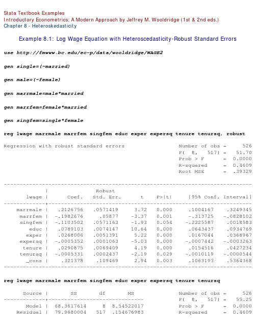
Stata Textbook ExamplesIntroductory Econometrics: A Modern Approach by Jeffrey M. Wooldridge (1st & 2nd eds.)Chapter 8 - HeteroskedasticityExample 8.1: Log Wage Equation with Heteroscedasticity-Robust Standard Errorsuse /ec-p/data/wooldridge/WAGE2gen single=(~married)gen male=(~female)gen marrmale=male*marriedgen marrfem=female*marriedgen singfem=single*femalereg lwage marrmale marrfem singfem educ exper expersq tenure tenursq, robustRegression with robust standard errors Number of obs = 526 F( 8, 517) = 51.70 Prob > F = 0.0000 R-squared = 0.4609 Root MSE = .39329------------------------------------------------------------------------------ | Robustlwage | Coef. Std. Err. t P>|t| [95% Conf. Interval] -------------+---------------------------------------------------------------- marrmale | .2126756 .0571419 3.72 0.000 .1004167 .3249345 marrfem | -.1982676 .05877 -3.37 0.001 -.313725 -.0828102 singfem | -.1103502 .0571163 -1.93 0.054 -.2225587 .0018583 educ | .0789103 .0074147 10.64 0.000 .0643437 .0934769 exper | .0268006 .0051391 5.22 0.000 .0167044 .0368967 expersq | -.0005352 .0001063 -5.03 0.000 -.0007442 -.0003263 tenure | .0290875 .0069409 4.19 0.000 .0154516 .0427234 tenursq | -.0005331 .0002437 -2.19 0.029 -.0010119 -.0000544 _cons | .321378 .109469 2.94 0.003 .1063193 .5364368 ------------------------------------------------------------------------------reg lwage marrmale marrfem singfem educ exper expersq tenure tenursqSource | SS df MS Number of obs = 526 -------------+------------------------------ F( 8, 517) = 55.25 Model | 68.3617614 8 8.54522017 Prob > F = 0.0000 Residual | 79.9680004 517 .154676983 R-squared = 0.4609Total | 148.329762 525 .28253288 Root MSE = .39329 ------------------------------------------------------------------------------ lwage | Coef. Std. Err. t P>|t| [95% Conf. Interval] -------------+---------------------------------------------------------------- marrmale | .2126756 .0553572 3.84 0.000 .103923 .3214283 marrfem | -.1982676 .0578355 -3.43 0.001 -.3118891 -.0846462 singfem | -.1103502 .0557421 -1.98 0.048 -.219859 -.0008414 educ | .0789103 .0066945 11.79 0.000 .0657585 .0920621 exper | .0268006 .0052428 5.11 0.000 .0165007 .0371005 expersq | -.0005352 .0001104 -4.85 0.000 -.0007522 -.0003183 tenure | .0290875 .006762 4.30 0.000 .0158031 .0423719 tenursq | -.0005331 .0002312 -2.31 0.022 -.0009874 -.0000789 _cons | .321378 .100009 3.21 0.001 .1249041 .517852 ------------------------------------------------------------------------------Example 8.2: Heteroscedastisity-Robust F Statisticsuse /ec-p/data/wooldridge/GPA3reg cumgpa sat hsperc tothrs female black white if term==2, robustRegression with robust standard errors Number of obs = 366 F( 6, 359) = 39.30 Prob > F = 0.0000 R-squared = 0.4006 Root MSE = .46929 ------------------------------------------------------------------------------ | Robustcumgpa | Coef. Std. Err. t P>|t| [95% Conf. Interval] -------------+---------------------------------------------------------------- sat | .0011407 .0001915 5.96 0.000 .0007641 .0015174 hsperc | -.0085664 .0014179 -6.04 0.000 -.0113548 -.0057779 tothrs | .002504 .0007406 3.38 0.001 .0010475 .0039605 female | .3034333 .0591378 5.13 0.000 .1871332 .4197334 black | -.1282837 .1192413 -1.08 0.283 -.3627829 .1062155 white | -.0587217 .111392 -0.53 0.598 -.2777846 .1603411 _cons | 1.470065 .2206802 6.66 0.000 1.036076 1.904053 ------------------------------------------------------------------------------reg cumgpa sat hsperc tothrs female black white if term==2Source | SS df MS Number of obs = 366Model | 52.831358 6 8.80522634 Prob > F = 0.0000 Residual | 79.062328 359 .220229326 R-squared = 0.4006 -------------+------------------------------ Adj R-squared = 0.3905 Total | 131.893686 365 .361352564 Root MSE = .46929 ------------------------------------------------------------------------------ cumgpa | Coef. Std. Err. t P>|t| [95% Conf. Interval] -------------+---------------------------------------------------------------- sat | .0011407 .0001786 6.39 0.000 .0007896 .0014919 hsperc | -.0085664 .0012404 -6.91 0.000 -.0110058 -.006127 tothrs | .002504 .000731 3.43 0.001 .0010664 .0039415 female | .3034333 .0590203 5.14 0.000 .1873643 .4195023 black | -.1282837 .1473701 -0.87 0.385 -.4181009 .1615335 white | -.0587217 .1409896 -0.42 0.677 -.3359909 .2185475 _cons | 1.470065 .2298031 6.40 0.000 1.018135 1.921994 ------------------------------------------------------------------------------Example 8.3: Heteroskedasticity-Robust LM Statisticuse /ec-p/data/wooldridge/CRIME1gen avgsensq=avgsen*avgsenreg narr86 pcnv avgsen avgsensq ptime86 qemp86 inc86 black hispan, robust Regression with robust standard errors Number of obs = 2725 F( 8, 2716) = 29.84 Prob > F = 0.0000 R-squared = 0.0728 Root MSE = .82843------------------------------------------------------------------------------ | Robustnarr86 | Coef. Std. Err. t P>|t| [95% Conf. Interval] -------------+---------------------------------------------------------------- pcnv | -.1355954 .0336218 -4.03 0.000 -.2015223 -.0696685 avgsen | .0178411 .0101233 1.76 0.078 -.0020091 .0376913 avgsensq | -.0005163 .0002077 -2.49 0.013 -.0009236 -.0001091 ptime86 | -.03936 .0062236 -6.32 0.000 -.0515634 -.0271566 qemp86 | -.0505072 .0142015 -3.56 0.000 -.078354 -.0226603 inc86 | -.0014797 .0002295 -6.45 0.000 -.0019297 -.0010296 black | .3246024 .0585135 5.55 0.000 .2098669 .439338 hispan | .19338 .0402983 4.80 0.000 .1143616 .2723985 _cons | .5670128 .0402756 14.08 0.000 .4880389 .6459867Source | SS df MS Number of obs = 2725 -------------+------------------------------ F( 2, 2723) = 2.00 Model | 3.99708536 2 1.99854268 Prob > F = 0.1355 Residual | 2721.00291 2723 .999266586 R-squared = 0.0015 -------------+------------------------------ Adj R-squared = 0.0007 Total | 2725.00 2725 1.00 Root MSE = .99963 ------------------------------------------------------------------------------ iota | Coef. Std. Err. t P>|t| [95% Conf. Interval] -------------+---------------------------------------------------------------- ur1 | .0277846 .0140598 1.98 0.048 .0002156 .0553537 ur2 | -.0010447 .0005479 -1.91 0.057 -.002119 .0000296 ------------------------------------------------------------------------------scalar hetlm = e(N)-e(rss)scalar pval = chi2tail(2,hetlm)display _n "Robust LM statistic : " %6.3f hetlm /*> */ _n "Under H0, distrib Chi2(2), p-value: " %5.3f pvalRobust LM statistic : 3.997Under H0, distrib Chi2(2), p-value: 0.136reg narr86 pcnv ptime86 qemp86 inc86 black hispanSource | SS df MS Number of obs = 2725 -------------+------------------------------ F( 6, 2718) = 34.95 Model | 143.977563 6 23.9962606 Prob > F = 0.0000 Residual | 1866.36959 2718 .686670196 R-squared = 0.0716 -------------+------------------------------ Adj R-squared = 0.0696 Total | 2010.34716 2724 .738012906 Root MSE = .82866 ------------------------------------------------------------------------------ narr86 | Coef. Std. Err. t P>|t| [95% Conf. Interval] -------------+---------------------------------------------------------------- pcnv | -.1322784 .0403406 -3.28 0.001 -.2113797 -.0531771 ptime86 | -.0377953 .008497 -4.45 0.000 -.0544566 -.021134 qemp86 | -.0509814 .0144359 -3.53 0.000 -.0792878 -.022675 inc86 | -.00149 .0003404 -4.38 0.000 -.0021575 -.0008224 black | .3296885 .0451778 7.30 0.000 .2411022 .4182748 hispan | .1954509 .0396929 4.92 0.000 .1176195 .2732823 _cons | .5703344 .0360073 15.84 0.000 .49973 .6409388 -----------------------------------------------------------------------------predict ubar2, residreg ubar2 pcnv avgsen avgsensq ptime86 qemp86 inc86 black hispanSource | SS df MS Number of obs = 2725 -------------+------------------------------ F( 8, 2716) = 0.43 Model | 2.37155739 8 .296444674 Prob > F = 0.9025 Residual | 1863.99804 2716 .686302664 R-squared = 0.0013 -------------+------------------------------ Adj R-squared = -0.0017 Total | 1866.36959 2724 .685157707 Root MSE = .82843 ------------------------------------------------------------------------------ ubar1 | Coef. Std. Err. t P>|t| [95% Conf. Interval] -------------+---------------------------------------------------------------- pcnv | -.003317 .0403699 -0.08 0.935 -.0824758 .0758418 avgsen | .0178411 .009696 1.84 0.066 -.0011713 .0368534 avgsensq | -.0005163 .000297 -1.74 0.082 -.0010987 .0000661 ptime86 | -.0015647 .0086935 -0.18 0.857 -.0186112 .0154819 qemp86 | .0004742 .0144345 0.03 0.974 -.0278295 .0287779 inc86 | .0000103 .0003405 0.03 0.976 -.0006574 .000678 black | -.0050861 .0454188 -0.11 0.911 -.094145 .0839729 hispan | -.0020709 .0397035 -0.05 0.958 -.0799229 .0757812 _cons | -.0033216 .0360573 -0.09 0.927 -.0740242 .0673809 ------------------------------------------------------------------------------scalar lm1 = e(N)*e(r2)display _n "LM statistic : " %6.3f lm1 /*LM statistic : 3.5425Example 8.4: Heteroscedasticity in Housing Price Equationuse /ec-p/data/wooldridge/HPRICE1reg price lotsize sqrft bdrmsSource | SS df MS Number of obs = 88 -------------+------------------------------ F( 3, 84) = 57.46 Model | 617130.701 3 205710.234 Prob > F = 0.0000 Residual | 300723.805 84 3580.0453 R-squared = 0.6724 -------------+------------------------------ Adj R-squared = 0.6607 Total | 917854.506 87 10550.0518 Root MSE = 59.833 ------------------------------------------------------------------------------ price | Coef. Std. Err. t P>|t| [95% Conf. Interval] -------------+----------------------------------------------------------------lotsize | .0020677 .0006421 3.22 0.002 .0007908 .0033446 sqrft | .1227782 .0132374 9.28 0.000 .0964541 .1491022 bdrms | 13.85252 9.010145 1.54 0.128 -4.06514 31.77018 _cons | -21.77031 29.47504 -0.74 0.462 -80.38466 36.84404 ------------------------------------------------------------------------------whitetst, fittedWhite's special test statistic : 16.26842 Chi-sq( 2) P-value = 2.9e-04reg lprice llotsize lsqrft bdrmsSource | SS df MS Number of obs = 88 -------------+------------------------------ F( 3, 84) = 50.42 Model | 5.15504028 3 1.71834676 Prob > F = 0.0000 Residual | 2.86256324 84 .034078134 R-squared = 0.6430 -------------+------------------------------ Adj R-squared = 0.6302 Total | 8.01760352 87 .092156362 Root MSE = .1846 ------------------------------------------------------------------------------ lprice | Coef. Std. Err. t P>|t| [95% Conf. Interval] -------------+---------------------------------------------------------------- llotsize | .1679667 .0382812 4.39 0.000 .0918404 .244093 lsqrft | .7002324 .0928652 7.54 0.000 .5155597 .8849051 bdrms | .0369584 .0275313 1.34 0.183 -.0177906 .0917074 _cons | -1.297042 .6512836 -1.99 0.050 -2.592191 -.0018931 ------------------------------------------------------------------------------whitetst, fittedWhite's special test statistic : 3.447243 Chi-sq( 2) P-value = .1784Example 8.5: Special Form of the White Test in the Log Housing Price Equationuse /ec-p/data/wooldridge/HPRICE1reg lprice llotsize lsqrft bdrmsSource | SS df MS Number of obs = 88 -------------+------------------------------ F( 3, 84) = 50.42 Model | 5.15506425 3 1.71835475 Prob > F = 0.0000 Residual | 2.86255771 84 .034078068 R-squared = 0.6430 -------------+------------------------------ Adj R-squared = 0.6302 Total | 8.01762195 87 .092156574 Root MSE = .1846llotsize | .167968 .0382811 4.39 0.000 .0918418 .2440941 lsqrft | .7002326 .0928652 7.54 0.000 .5155601 .8849051 bdrms | .0369585 .0275313 1.34 0.183 -.0177905 .0917075 _cons | 5.6107 .6512829 8.61 0.000 4.315553 6.905848 ------------------------------------------------------------------------------whitetst, fittedWhite's special test statistic : 3.447286 Chi-sq( 2) P-value = .1784Example 8.6: Family Saving Equationuse /ec-p/data/wooldridge/SAVINGreg sav incSource | SS df MS Number of obs = 100 -------------+------------------------------ F( 1, 98) = 6.49 Model | 66368437.0 1 66368437.0 Prob > F = 0.0124 Residual | 1.0019e+09 98 10223460.8 R-squared = 0.0621 -------------+------------------------------ Adj R-squared = 0.0526 Total | 1.0683e+09 99 10790581.8 Root MSE = 3197.4 ------------------------------------------------------------------------------ sav | Coef. Std. Err. t P>|t| [95% Conf. Interval] -------------+---------------------------------------------------------------- inc | .1466283 .0575488 2.55 0.012 .0324247 .260832 _cons | 124.8424 655.3931 0.19 0.849 -1175.764 1425.449 ------------------------------------------------------------------------------reg sav inc [aw = 1/inc](sum of wgt is 1.3877e-02)Source | SS df MS Number of obs = 100 -------------+------------------------------ F( 1, 98) = 9.14 Model | 58142339.8 1 58142339.8 Prob > F = 0.0032 Residual | 623432468 98 6361555.80 R-squared = 0.0853 -------------+------------------------------ Adj R-squared = 0.0760 Total | 681574808 99 6884594.02 Root MSE = 2522.2inc | .1717555 .0568128 3.02 0.003 .0590124 .2844986 _cons | -124.9528 480.8606 -0.26 0.796 -1079.205 829.2994 ------------------------------------------------------------------------------reg sav inc size educ age blackSource | SS df MS Number of obs = 100 -------------+------------------------------ F( 5, 94) = 1.70 Model | 88426246.4 5 17685249.3 Prob > F = 0.1430 Residual | 979841351 94 10423844.2 R-squared = 0.0828 -------------+------------------------------ Adj R-squared = 0.0340 Total | 1.0683e+09 99 10790581.8 Root MSE = 3228.6 ------------------------------------------------------------------------------ sav | Coef. Std. Err. t P>|t| [95% Conf. Interval] -------------+---------------------------------------------------------------- inc | .109455 .0714317 1.53 0.129 -.0323742 .2512842 size | 67.66119 222.9642 0.30 0.762 -375.0395 510.3619 educ | 151.8235 117.2487 1.29 0.199 -80.97646 384.6235 age | .2857217 50.03108 0.01 0.995 -99.05217 99.62361 black | 518.3934 1308.063 0.40 0.693 -2078.796 3115.583 _cons | -1605.416 2830.707 -0.57 0.572 -7225.851 4015.019 ------------------------------------------------------------------------------reg sav inc size educ age black [aw = 1/inc](sum of wgt is 1.3877e-02)Source | SS df MS Number of obs = 100 -------------+------------------------------ F( 5, 94) = 2.19 Model | 71020334.9 5 14204067.0 Prob > F = 0.0621 Residual | 610554473 94 6495260.35 R-squared = 0.1042 -------------+------------------------------ Adj R-squared = 0.0566 Total | 681574808 99 6884594.02 Root MSE = 2548.6 ------------------------------------------------------------------------------ sav | Coef. Std. Err. t P>|t| [95% Conf. Interval] -------------+---------------------------------------------------------------- inc | .1005179 .0772511 1.30 0.196 -.052866 .2539017 size | -6.868501 168.4327 -0.04 0.968 -341.2956 327.5586 educ | 139.4802 100.5362 1.39 0.169 -60.1368 339.0972 age | 21.74721 41.30598 0.53 0.600 -60.26678 103.7612 black | 137.2842 844.5941 0.16 0.871 -1539.677 1814.246 _cons | -1854.814 2351.797 -0.79 0.432 -6524.362 2814.734 ------------------------------------------------------------------------------Example 8.7: Demand for Cigarettesuse /ec-p/data/wooldridge/SMOKEreg cigs lincome lcigpric educ age agesq restaurnSource | SS df MS Number of obs = 807 -------------+------------------------------ F( 6, 800) = 7.42 Model | 8003.02506 6 1333.83751 Prob > F = 0.0000 Residual | 143750.658 800 179.688322 R-squared = 0.0527 -------------+------------------------------ Adj R-squared = 0.0456 Total | 151753.683 806 188.280003 Root MSE = 13.405 ------------------------------------------------------------------------------ cigs | Coef. Std. Err. t P>|t| [95% Conf. Interval] -------------+---------------------------------------------------------------- lincome | .8802689 .7277838 1.21 0.227 -.5483223 2.30886 lcigpric | -.7508498 5.773343 -0.13 0.897 -12.08354 10.58184 educ | -.5014982 .1670772 -3.00 0.003 -.8294597 -.1735368 age | .7706936 .1601223 4.81 0.000 .456384 1.085003 agesq | -.0090228 .001743 -5.18 0.000 -.0124443 -.0056013 restaurn | -2.825085 1.111794 -2.54 0.011 -5.007462 -.642708 _cons | -3.639884 24.07866 -0.15 0.880 -50.9047 43.62493 ------------------------------------------------------------------------------Change in cigs if income increases by 10%display _b[lincome]*10/100.08802689Turnover point for agedisplay _b[age]/2/_b[agesq]-42.708116whitetst, fittedWhite's special test statistic : 26.57258 Chi-sq( 2) P-value = 1.7e-06gen lubar=log(ub*ub)qui reg lubar lincome lcigpric educ age agesq restaurnpredict cigsh, xbgen cigse = exp(cigsh)reg cigs lincome lcigpric educ age agesq restaurn [aw=1/cigse](sum of wgt is 1.9977e+01)Source | SS df MS Number of obs = 807 -------------+------------------------------ F( 6, 800) = 17.06 Model | 10302.6415 6 1717.10692 Prob > F = 0.0000 Residual | 80542.0684 800 100.677586 R-squared = 0.1134 -------------+------------------------------ Adj R-squared = 0.1068 Total | 90844.71 806 112.710558 Root MSE = 10.034 ------------------------------------------------------------------------------ cigs | Coef. Std. Err. t P>|t| [95% Conf. Interval] -------------+---------------------------------------------------------------- lincome | 1.295241 .4370118 2.96 0.003 .4374154 2.153066 lcigpric | -2.94028 4.460142 -0.66 0.510 -11.69524 5.814684 educ | -.4634462 .1201586 -3.86 0.000 -.6993095 -.2275829 age | .4819474 .0968082 4.98 0.000 .2919194 .6719755 agesq | -.0056272 .0009395 -5.99 0.000 -.0074713 -.0037831 restaurn | -3.461066 .7955047 -4.35 0.000 -5.022589 -1.899543 _cons | 5.63533 17.80313 0.32 0.752 -29.31103 40.58169 ------------------------------------------------------------------------------Example 8.8: Labor Force Participation of Married Womenuse /ec-p/data/wooldridge/MROZreg inlf nwifeinc educ exper expersq age kidslt6 kidsge6Source | SS df MS Number of obs = 753 -------------+------------------------------ F( 7, 745) = 38.22 Model | 48.8080578 7 6.97257968 Prob > F = 0.0000 Residual | 135.919698 745 .182442547 R-squared = 0.2642 -------------+------------------------------ Adj R-squared = 0.2573 Total | 184.727756 752 .245648611 Root MSE = .42713 ------------------------------------------------------------------------------ inlf | Coef. Std. Err. t P>|t| [95% Conf. Interval] -------------+---------------------------------------------------------------- nwifeinc | -.0034052 .0014485 -2.35 0.019 -.0062488 -.0005616 educ | .0379953 .007376 5.15 0.000 .023515 .0524756exper | .0394924 .0056727 6.96 0.000 .0283561 .0506287 expersq | -.0005963 .0001848 -3.23 0.001 -.0009591 -.0002335 age | -.0160908 .0024847 -6.48 0.000 -.0209686 -.011213 kidslt6 | -.2618105 .0335058 -7.81 0.000 -.3275875 -.1960335 kidsge6 | .0130122 .013196 0.99 0.324 -.0128935 .0389179 _cons | .5855192 .154178 3.80 0.000 .2828442 .8881943 ------------------------------------------------------------------------------reg inlf nwifeinc educ exper expersq age kidslt6 kidsge6, robustRegression with robust standard errors Number of obs = 753 F( 7, 745) = 62.48 Prob > F = 0.0000 R-squared = 0.2642 Root MSE = .42713 ------------------------------------------------------------------------------ | Robustinlf | Coef. Std. Err. t P>|t| [95% Conf. Interval] -------------+---------------------------------------------------------------- nwifeinc | -.0034052 .0015249 -2.23 0.026 -.0063988 -.0004115 educ | .0379953 .007266 5.23 0.000 .023731 .0522596 exper | .0394924 .00581 6.80 0.000 .0280864 .0508983 expersq | -.0005963 .00019 -3.14 0.002 -.0009693 -.0002233 age | -.0160908 .002399 -6.71 0.000 -.0208004 -.0113812 kidslt6 | -.2618105 .0317832 -8.24 0.000 -.3242058 -.1994152 kidsge6 | .0130122 .0135329 0.96 0.337 -.013555 .0395795 _cons | .5855192 .1522599 3.85 0.000 .2866098 .8844287 ------------------------------------------------------------------------------Example 8.9: Determinants of Personal Computer Ownershipuse /ec-p/data/wooldridge/GPA1gen parcoll = (mothcoll | fathcoll)reg PC hsGPA ACT parcollSource | SS df MS Number of obs = 141 -------------+------------------------------ F( 3, 137) = 1.98 Model | 1.40186813 3 .467289377 Prob > F = 0.1201 Residual | 32.3569971 137 .236182461 R-squared = 0.0415 -------------+------------------------------ Adj R-squared = 0.0205 Total | 33.7588652 140 .241134752 Root MSE = .48599------------------------------------------------------------------------------ PC | Coef. Std. Err. t P>|t| [95% Conf. Interval] -------------+---------------------------------------------------------------- hsGPA | .0653943 .1372576 0.48 0.635 -.2060231 .3368118 ACT | .0005645 .0154967 0.04 0.971 -.0300792 .0312082 parcoll | .2210541 .092957 2.38 0.019 .037238 .4048702 _cons | -.0004322 .4905358 -0.00 0.999 -.970433 .9695686 ------------------------------------------------------------------------------predict phatgen h=phat*(1-phat)reg PC hsGPA ACT parcoll [aw=1/h](sum of wgt is 6.2818e+02)Source | SS df MS Number of obs = 141 -------------+------------------------------ F( 3, 137) = 2.22 Model | 1.54663033 3 .515543445 Prob > F = 0.0882 Residual | 31.7573194 137 .231805251 R-squared = 0.0464 -------------+------------------------------ Adj R-squared = 0.0256 Total | 33.3039497 140 .237885355 Root MSE = .48146 ------------------------------------------------------------------------------ PC | Coef. Std. Err. t P>|t| [95% Conf. Interval] -------------+---------------------------------------------------------------- hsGPA | .0327029 .1298817 0.25 0.802 -.2241292 .289535 ACT | .004272 .0154527 0.28 0.783 -.0262847 .0348286 parcoll | .2151862 .0862918 2.49 0.014 .04455 .3858224 _cons | .0262099 .4766498 0.05 0.956 -.9163323 .9687521 ------------------------------------------------------------------------------This page prepared by Oleksandr Talavera (revised 8 Nov 2002)Send your questions/comments/suggestions to Kit Baum at baum@ These pages are maintained by the Faculty Micro Resource Center's GSA Program,a unit of Boston College Academic Technology Services。
Introduction-to-Finite-Elements-Method

; ; ;
IFEM Ch 1–Slide 12
; ; ;
Introduction to FEM
Two Interpretations of FEM for Teaching
Physical
Breakdown of structural system into components (elements) and reconstruction by the assembly process Emphasized in Part I
IFEM Ch 1–Slide 3
Introduction to FEM
Computational Mechanics
Branches of Computational Mechanics can be distinguished according to the physical focus of attention
Introduction to FEM
FEM in Modeling and Simulation: Mathematical FEM
Mathematical model
IDEALIZATION REALIZATION
Discretization + solution error
FEM
SOLUTION
3 4 2 4
r d
5 1 5
2r sin(π/n) i
2π/n 6 7 8
j r
IFEM Ch 1–Slide 10
Introduction to FEM
Computing π "by Archimedes FEM"
n 1 2 4 8 16 32 64 128 256
整车FEM建模手册绝密

整车FEM建模手册-绝密用于碰撞被动安全性CAE分析FEM建模手册车身模型建模要求一般要求General Requirements1. The parts shall be modelled using linear (3 or 4 noded) shell elements.2. The parts shall be modelled on the mid surface. If the delivered geometry is not a mid surface representation, the geometry shall be modified to represent the mid surface.3. No elements are allowed to cross the “symmetry” line y=0 (nodes shall be positioned on y=0)4. The shell elements shall be consistently defined.5. The parts shall be modelled in the following unit settings:• Length in millimetres (mm)• Time in second (s)• Mass in tonne• Force in Newton6. Each part shall have one unique PID, with the following exceptions: • Parts made of tailored blanks shall be divided into different PIDs according to thedifferent thickness and material qualities of the parts.• Extruded parts shall be divided into different PIDs according to the differentthickness and materials of extrusion.• The thickness at different locations on a cast/moulded part7. The preferred naming convention as below:ST3700=1234567_A1A_3.5_B-Pillarmaterial drawing no drawing rev thickness part name8. All parts with identical materials properties shall refer to the same MID.9. One model shall be used for all crash simulation建模要求Meshing Guideline1. Deformation area shall be mesh with a average length 10mm. Deformation area shall be mesh with a minimum length of not less than 5mm. Maximum length shall not exceed 12mm.注:变形区域:正面碰撞:A柱与B柱中间位置以前的所有零件及其某些零件的前部(车门除外),另外前端吸能部件,包括纵梁前段、翼子板支撑结构等的平均单元长度为8 mm;侧面碰撞:前后从A柱至C柱(包括A柱与C柱),横向左半部所有零件及其某些零件的左半部(框内的零件及其某些零件的框内部分);背面碰撞:C立柱(包括C立柱)以后的所有零件及其某些零件的后部(车门除外)。
海上油气泄漏与扩散场景数值分析

海上油气泄漏与扩散场景数值分析闫会宾 1,2,薛鸿祥 1,2,唐文勇 1,2(1.上海交通大学海洋工程国家重点实验室,上海 200240;2.高新船舶与深海开发装备协同创新中心,上海 200240)摘要:海上油气装置发生气体泄漏并经过一定程度扩散后极易被点燃而发生爆炸事故。
该文针对一个海上油气处理 模块选取多组不同泄漏速率与风速组合下的泄漏扩散场景建立 CFD 模型进行分析,深入讨论了气体浓度的分布与形 成规律,并选取可用于爆炸分析的重要指标“等效化学计量气体云体积”作为分析对象,深入分析其随时间的变化规律, 发现气体扩散后的浓度分布均可以在一定时间后达到稳定状态,等效化学计量气体云体积不再变化;另外还探讨了 泄漏速率以及风速等关键参数对特征气体云体积的大小以及形成时间的影响规律,获得的相关规律可用于类似场景 的参考;最后对爆炸分析时泄漏扩散场景的选择提出了相关建议。
关键词:海上油气装置;泄漏;扩散;等效可燃气体云;CFD 中图分类号(小五黑):P754 文献标识码(小五黑):ANumerical analysis of hydrocarbon leakand dispersion in offshore oil & gas installationsHuibin Yan1,2, Wenyong Tang1,2, Hongxiang Xue1,21State Key Laboratory of Ocean Engineering, Shanghai Jiao Tong University, Shanghai 200240,china; 2 Collaborative Innovation Center for Advanced Ship and Deep-Sea Exploration, Shanghai 200240,china. Abstract: if a hydrocarbon leak happened in an offshore oil & gas installation and dispersed with a certain time, it would be of high possibility to be ignited and lead to an explosion accident, which needs to be studied thoroughly. In this paper, CFD theory based FLACS code was chosen to do dispersion analysis for multi-group of leak scenarios in an example offshore oil & gas installationwith different leak rates and wind speeds. The distribution and evolution laws of the gas concentration in the considered zone were studied; the “equivalent stoichiometric gas volume” of each scenario, which is a key parameter to explosion analysis, was chosen to study its evolution law with time; the effect of leak rate and wind speed on the key characteristics of “equivalent stoichiometric gas volume” was discussed in detail; at last, some valuable suggestions about defining leak and dispersion scenarios for explosion accidents were given. Key words: offshore oil & gas installation; leak; dispersion; equivalent stoichiometric gas volume; CFD0引 言油气作为一种石化产品的总称,主要是指液态的油与气态的各种介质,均属于易燃易爆物,且 部分有毒。
fem关键参数 -回复

fem关键参数-回复“fem关键参数”是指有限元方法(finite element method, FEM)中的重要参数。
有限元方法是一种在工程学和科学计算中广泛使用的数值分析技术,用于解决各种工程问题和物理问题。
在使用有限元方法进行数值模拟时,正确选择和调节关键参数是至关重要的,以确保模拟结果的准确性和可靠性。
本文将以“fem关键参数”为主题,一步一步回答。
第1步:什么是有限元方法?有限元方法是一种数值分析技术,用于通过将复杂的连续体分割成简单的有限元(如三角形、四边形或六面体等)来近似求解偏微分方程。
该方法基于分割后的有限元之间的关系建立方程,通过求解这些方程来获得所需的物理量。
有限元方法可以用于解决各种问题,包括结构力学、流体力学、电磁场等。
第2步:有限元方法中的关键参数有哪些?在有限元方法中,有几个关键参数需要正确选择和调节,以确保模拟结果的准确性和可靠性。
以下是其中的几个关键参数:1. 网格大小:网格的大小决定了有限元模型的精度和计算效率。
较小的网格将提供更准确的结果,但计算成本也更高。
因此,需要根据具体问题的需求在准确性和计算效率之间进行权衡。
2. 单元类型:有限元方法中的单元可以是多边形、三角形、四边形或六边形等。
正确选择适当的单元类型可以确保模拟结果的准确性。
对于具有复杂几何形状的问题,可能需要使用高阶单元或非结构化网格。
3. 材料参数:材料参数包括弹性模量、泊松比、密度等物理性质。
正确选择和调节材料参数对于模拟结果的准确性至关重要。
这些参数可以通过实验测试获得,也可以通过其他模拟方法进行估计。
4. 边界条件:边界条件定义了问题的边界上的约束和加载情况。
正确定义边界条件对于模拟结果的准确性至关重要。
边界条件可以是位移、力、热流等。
5. 数值积分:有限元方法中的数值积分用于将连续的物理量转化为离散的近似值。
正确选择适当的数值积分方法可以提高模拟结果的准确性。
对于复杂的几何形状和显著变化的物理量,可能需要使用高阶数值积分方法。
2024届高三英语基础写作:邀请外教参加重阳节活动+课件

13. What does the underlined phrase “pored over” in paragraph 3 probably mean?
A. Copied.
ቤተ መጻሕፍቲ ባይዱ
B. Covered.
C. Studied.
D. Borrowed.
2024届新高三摸底联考
英语
第二部分 语言运用(共两节,满分30分)
We deal in hardware but not software. 我们只经营硬件而不经营软件。 2) (贬义) concern oneself with sth; indulge in sth 忙於某事物; 沉溺於某事物 deal in gossip
share (in) sth. 分摊或分享某事物; 参与某事物 I will share (in) the cost with you. 我愿与你分摊费用。 She shares (in) my troubles as well as my joys. 她与我同甘共苦。
2024届新高三摸底联考
英语
第二节 (共10小题;每小题1.5分,满分15分)
阅读下面短文,在空白处填入1个适当的单词或括号内单词的正确形式。
Movies could serve as a valuable “classroom” for children to explore into the
culture and history of their own country. A new book 36. collecting .(collect) 20
take in
He was homeless, so we took him in. 他无家可归, 我们就收留了他。 She took me in completely with her story. 她用谎话把我完全蒙蔽了。 Don’t be taken in by his charming manner; he’s completely ruthless. 不要被他那副讨人喜欢的外表所迷惑, 其实他冷酷无情。 Fish take in oxygen through their gills. 鱼通过鳃摄取氧气。 He took in every detail of her appearance. 他端详了她一番。 He took in the scene at a glance. 他看了一眼那里的景色。 I hope you’re taking in what I’m saying. 我希望你能听得进去我说的话。