DigitalImageProcessing5-ImageEnhancement(HistogramProcessing)
数字图像处理 第三版 (冈萨雷斯,自己整理的1)
1.1 图像与图像处理的概念图像(Image):使用各种观测系统以不同形式和手段观测客观世界而获得的,可以直接或间接作用于人眼并进而产生视觉的实体。
包括:·各类图片,如普通照片、X光片、遥感图片;·各类光学图像,如电影、电视画面;·客观世界在人们心目中的有形想象以及外部描述,如绘画、绘图等。
数字图像:为了能用计算机对图像进行加工,需要把连续图像在坐标空间和性质空间都离散化,这种离散化了的图像是数字图像。
图像中每个基本单元叫做图像的元素,简称像素(Pixel)。
数字图像处理(Digital Image Processing):是指应用计算机来合成、变换已有的数字图像,从而产生一种新的效果,并把加工处理后的图像重新输出,这个过程称为数字图像处理。
也称之为计算机图像处理(Computer Image Processing)。
1.2 图像处理科学的意义1.图像是人们从客观世界获取信息的重要来源·人类是通过感觉器官从客观世界获取信息的,即通过耳、目、口、鼻、手通过听、看、味、嗅和接触的方式获取信息。
在这些信息中,视觉信息占70%。
·视觉信息的特点是信息量大,传播速度快,作用距离远,有心理和生理作用,加上大脑的思维和联想,具有很强的判断能力。
·人的视觉十分完善,人眼灵敏度高,鉴别能力强,不仅可以辨别景物,还能辨别人的情绪。
2.图像信息处理是人类视觉延续的重要手段非可见光成像。
如:γ射线、X射线、紫外线、红外线、微波。
利用图像处理技术把这些不可见射线所成图像加以处理并转换成可见图像,可对非人类习惯的那些图像源进行加工。
3.图像处理技术对国计民生有重大意义图像处理技术发展到今天,许多技术已日益趋于成熟,应用也越来越广泛。
它渗透到许多领域,如遥感、生物医学、通信、工业、航空航天、军事、安全保卫等。
1.3 数字图像处理的特点1. 图像信息量大每个像素的灰度级至少要用6bit(单色图像)来表示,一般采用8bit(彩色图像),高精度的可用12bit 或16bit。
15Digital image processing

Digital image processing数字图像处理第一章1、Digital image processing is the use of a digital computer to process digital images through an algorithm.数字图像处理是将图像信号转换成数字信号并利用计算机对其进行处理的过程。
2、Images can be divided into two types:analog images and digital images.Analog image refers to the image that shows color through objective physical quantity.Its space coordinate value x and y are continuous,and the light intensity at each space point(x,y)is also continuous,which cannot be processed by computer.The analog image is digitized to get the digital image,which can be stored and processed by the computer.A digital image consists of a finite number of elements,each of which has its spatial position(x,y)and intensity value f quantified into discrete values,called pixels.Digital images are two-dimensional pixel matrices with discrete values that can be stored in computer memory.图像可以分为两种类型:模拟图像和数字图像。
边缘检测中英文翻译
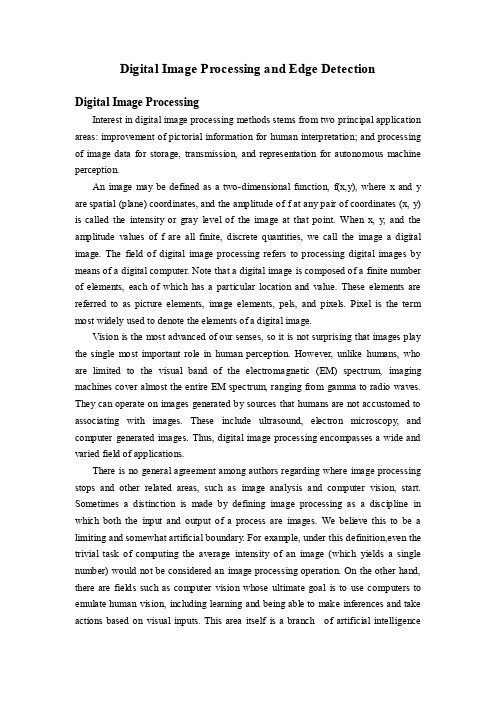
Digital Image Processing and Edge DetectionDigital Image ProcessingInterest in digital image processing methods stems from two principal application areas: improvement of pictorial information for human interpretation; and processing of image data for storage, transmission, and representation for autonomous machine perception.An image may be defined as a two-dimensional function, f(x,y), where x and y are spatial (plane) coordinates, and the amplitude of f at any pair of coordinates (x, y) is called the intensity or gray level of the image at that point. When x, y, and the amplitude values of f are all finite, discrete quantities, we call the image a digital image. The field of digital image processing refers to processing digital images by means of a digital computer. Note that a digital image is composed of a finite number of elements, each of which has a particular location and value. These elements are referred to as picture elements, image elements, pels, and pixels. Pixel is the term most widely used to denote the elements of a digital image.Vision is the most advanced of our senses, so it is not surprising that images play the single most important role in human perception. However, unlike humans, who are limited to the visual band of the electromagnetic (EM) spectrum, imaging machines cover almost the entire EM spectrum, ranging from gamma to radio waves. They can operate on images generated by sources that humans are not accustomed to associating with images. These include ultrasound, electron microscopy, and computer generated images. Thus, digital image processing encompasses a wide and varied field of applications.There is no general agreement among authors regarding where image processing stops and other related areas, such as image analysis and computer vision, start. Sometimes a distinction is made by defining image processing as a discipline in which both the input and output of a process are images. We believe this to be a limiting and somewhat artificial boundary. For example, under this definition,even the trivial task of computing the average intensity of an image (which yields a single number) would not be considered an image processing operation. On the other hand, there are fields such as computer vision whose ultimate goal is to use computers to emulate human vision, including learning and being able to make inferences and take actions based on visual inputs. This area itself is a branch of artificial intelligence(AI) whose objective is to emulate human intelligence. The field of AI is in its earliest stages of infancy in terms of development, with progress having been much slower than originally anticipated. The area of image analysis (also called image understanding) is in between image processing and computer vision.There are no clearcut boundaries in the continuum from image processing at one end to computer vision at the other. However, one useful paradigm is to consider three types of computerized processes in this continuum: low, mid, and highlevel processes. Low-level processes involve primitive operations such as image preprocessing to reduce noise, contrast enhancement, and image sharpening. A low-level process is characterized by the fact that both its inputs and outputs are images. Mid-level processing on images involves tasks such as segmentation (partitioning an image into regions or objects), description of those objects to reduce them to a form suitable for computer processing, and classification (recognition) of individual objects. A midlevel process is characterized by the fact that its inputs generally are images, but its outputs are attributes extracted from those images (e.g., edges, contours, and the identity of individual objects). Finally, higherlevel processing involves “making sense” of an ensemble of recognize d objects, as in image analysis, and, at the far end of the continuum, performing the cognitive functions normally associated with vision.Based on the preceding comments, we see that a logical place of overlap between image processing and image analysis is the area of recognition of individual regions or objects in an image. Thus, what we call in this book digital image processing encompasses processes whose inputs and outputs are images and, in addition, encompasses processes that extract attributes from images, up to and including the recognition of individual objects. As a simple illustration to clarify these concepts, consider the area of automated analysis of text. The processes of acquiring an image of the area containing the text, preprocessing that image, extracting (segmenting) the individual characters, describing the characters in a form suitable for computer processing, and recognizing those individual characters are in the scope of what we call digital image processing in this book. Making sense of the content of the page may be viewed as being in the domain of image analysis and even computer vision, depending on the level of complexity implied by the statement “making sense.” As will become evident shortly, digital image processing, as we have defined it, is used successfully in a broad range of areas of exceptional social and economic value.The areas of application of digital image processing are so varied that some formof organization is desirable in attempting to capture the breadth of this field. One of the simplest ways to develop a basic understanding of the extent of image processing applications is to categorize images according to their source (e.g., visual, X-ray, and so on). The principal energy source for images in use today is the electromagnetic energy spectrum. Other important sources of energy include acoustic, ultrasonic, and electronic (in the form of electron beams used in electron microscopy). Synthetic images, used for modeling and visualization, are generated by computer. In this section we discuss briefly how images are generated in these various categories and the areas in which they are applied.Images based on radiation from the EM spectrum are the most familiar, especially images in the X-ray and visual bands of the spectrum. Electromagnetic waves can be conceptualized as propagating sinusoidal waves of varying wavelengths, or they can be thought of as a stream of massless particles, each traveling in a wavelike pattern and moving at the speed of light. Each massless particle contains a certain amount (or bundle) of energy. Each bundle of energy is called a photon. If spectral bands are grouped according to energy per photon, we obtain the spectrum shown in fig. below, ranging from gamma rays (highest energy) at one end to radio waves (lowest energy) at the other. The bands are shown shaded to convey the fact that bands of the EM spectrum are not distinct but rather transition smoothly from one to the other.Fig1Image acquisition is the first process. Note that acquisition could be as simple as being given an image that is already in digital form. Generally, the image acquisition stage involves preprocessing, such as scaling.Image enhancement is among the simplest and most appealing areas of digital image processing. Basically, the idea behind enhancement techniques is to bring out detail that is obscured, or simply to highlight certain features of interest in an image.A familiar example of enhancement is when we increase the contrast of an imagebecause “it looks better.” It is important to keep in mind that enhancement is a very subjective area of image processing. Image restoration is an area that also deals with improving the appearance of an image. However, unlike enhancement, which is subjective, image restoration is objective, in the sense that restoration techniques tend to be based on mathematical or probabilistic models of image degradation. Enhancement, on the other hand, is based on human subjective preferences regarding what constitutes a “good” en hancement result.Color image processing is an area that has been gaining in importance because of the significant increase in the use of digital images over the Internet. It covers a number of fundamental concepts in color models and basic color processing in a digital domain. Color is used also in later chapters as the basis for extracting features of interest in an image.Wavelets are the foundation for representing images in various degrees of resolution. In particular, this material is used in this book for image data compression and for pyramidal representation, in which images are subdivided successively into smaller regions.F ig2Compression, as the name implies, deals with techniques for reducing the storage required to save an image, or the bandwidth required to transmi it.Although storagetechnology has improved significantly over the past decade, the same cannot be said for transmission capacity. This is true particularly in uses of the Internet, which are characterized by significant pictorial content. Image compression is familiar (perhaps inadvertently) to most users of computers in the form of image file extensions, such as the jpg file extension used in the JPEG (Joint Photographic Experts Group) image compression standard.Morphological processing deals with tools for extracting image components that are useful in the representation and description of shape. The material in this chapter begins a transition from processes that output images to processes that output image attributes.Segmentation procedures partition an image into its constituent parts or objects. In general, autonomous segmentation is one of the most difficult tasks in digital image processing. A rugged segmentation procedure brings the process a long way toward successful solution of imaging problems that require objects to be identified individually. On the other hand, weak or erratic segmentation algorithms almost always guarantee eventual failure. In general, the more accurate the segmentation, the more likely recognition is to succeed.Representation and description almost always follow the output of a segmentation stage, which usually is raw pixel data, constituting either the boundary of a region (i.e., the set of pixels separating one image region from another) or all the points in the region itself. In either case, converting the data to a form suitable for computer processing is necessary. The first decision that must be made is whether the data should be represented as a boundary or as a complete region. Boundary representation is appropriate when the focus is on external shape characteristics, such as corners and inflections. Regional representation is appropriate when the focus is on internal properties, such as texture or skeletal shape. In some applications, these representations complement each other. Choosing a representation is only part of the solution for transforming raw data into a form suitable for subsequent computer processing. A method must also be specified for describing the data so that features of interest are highlighted. Description, also called feature selection, deals with extracting attributes that result in some quantitative information of interest or are basic for differentiating one class of objects from another.Recognition is the pro cess that assigns a label (e.g., “vehicle”) to an object based on its descriptors. As detailed before, we conclude our coverage of digital imageprocessing with the development of methods for recognition of individual objects.So far we have said nothing about the need for prior knowledge or about the interaction between the knowledge base and the processing modules in Fig2 above. Knowledge about a problem domain is coded into an image processing system in the form of a knowledge database. This knowledge may be as simple as detailing regions of an image where the information of interest is known to be located, thus limiting the search that has to be conducted in seeking that information. The knowledge base also can be quite complex, such as an interrelated list of all major possible defects in a materials inspection problem or an image database containing high-resolution satellite images of a region in connection with change-detection applications. In addition to guiding the operation of each processing module, the knowledge base also controls the interaction between modules. This distinction is made in Fig2 above by the use of double-headed arrows between the processing modules and the knowledge base, as opposed to single-headed arrows linking the processing modules.Edge detectionEdge detection is a terminology in image processing and computer vision, particularly in the areas of feature detection and feature extraction, to refer to algorithms which aim at identifying points in a digital image at which the image brightness changes sharply or more formally has discontinuities.Although point and line detection certainly are important in any discussion on segmentation,edge dectection is by far the most common approach for detecting meaningful discounties in gray level.Although certain literature has considered the detection of ideal step edges, the edges obtained from natural images are usually not at all ideal step edges. Instead they are normally affected by one or several of the following effects:1.focal b lur caused by a finite depth-of-field and finite point spread function; 2.penumbral blur caused by shadows created by light sources of non-zero radius; 3.shading at a smooth object edge; 4.local specularities or interreflections in the vicinity of object edges.A typical edge might for instance be the border between a block of red color and a block of yellow. In contrast a line (as can be extracted by a ridge detector) can be a small number of pixels of a different color on an otherwise unchanging background. For a line, there may therefore usually be one edge on each side of the line.To illustrate why edge detection is not a trivial task, let us consider the problemof detecting edges in the following one-dimensional signal. Here, we may intuitively say that there should be an edge between the 4th and 5th pixels.If the intensity difference were smaller between the 4th and the 5th pixels and if the intensity differences between the adjacent neighbouring pixels were higher, it would not be as easy to say that there should be an edge in the corresponding region. Moreover, one could argue that this case is one in which there are several edges.Hence, to firmly state a specific threshold on how large the intensity change between two neighbouring pixels must be for us to say that there should be an edge between these pixels is not always a simple problem. Indeed, this is one of the reasons why edge detection may be a non-trivial problem unless the objects in the scene are particularly simple and the illumination conditions can be well controlled.There are many methods for edge detection, but most of them can be grouped into two categories,search-based and zero-crossing based. The search-based methods detect edges by first computing a measure of edge strength, usually a first-order derivative expression such as the gradient magnitude, and then searching for local directional maxima of the gradient magnitude using a computed estimate of the local orientation of the edge, usually the gradient direction. The zero-crossing based methods search for zero crossings in a second-order derivative expression computed from the image in order to find edges, usually the zero-crossings of the Laplacian or the zero-crossings of a non-linear differential expression, as will be described in the section on differential edge detection following below. As a pre-processing step to edge detection, a smoothing stage, typically Gaussian smoothing, is almost always applied (see also noise reduction).The edge detection methods that have been published mainly differ in the types of smoothing filters that are applied and the way the measures of edge strength are computed. As many edge detection methods rely on the computation of image gradients, they also differ in the types of filters used for computing gradient estimates in the x- and y-directions.Once we have computed a measure of edge strength (typically the gradient magnitude), the next stage is to apply a threshold, to decide whether edges are present or not at an image point. The lower the threshold, the more edges will be detected, and the result will be increasingly susceptible to noise, and also to picking outirrelevant features from the image. Conversely a high threshold may miss subtle edges, or result in fragmented edges.If the edge thresholding is applied to just the gradient magnitude image, the resulting edges will in general be thick and some type of edge thinning post-processing is necessary. For edges detected with non-maximum suppression however, the edge curves are thin by definition and the edge pixels can be linked into edge polygon by an edge linking (edge tracking) procedure. On a discrete grid, the non-maximum suppression stage can be implemented by estimating the gradient direction using first-order derivatives, then rounding off the gradient direction to multiples of 45 degrees, and finally comparing the values of the gradient magnitude in the estimated gradient direction.A commonly used approach to handle the problem of appropriate thresholds for thresholding is by using thresholding with hysteresis. This method uses multiple thresholds to find edges. We begin by using the upper threshold to find the start of an edge. Once we have a start point, we then trace the path of the edge through the image pixel by pixel, marking an edge whenever we are above the lower threshold. We stop marking our edge only when the value falls below our lower threshold. This approach makes the assumption that edges are likely to be in continuous curves, and allows us to follow a faint section of an edge we have previously seen, without meaning that every noisy pixel in the image is marked down as an edge. Still, however, we have the problem of choosing appropriate thresholding parameters, and suitable thresholding values may vary over the image.Some edge-detection operators are instead based upon second-order derivatives of the intensity. This essentially captures the rate of change in the intensity gradient. Thus, in the ideal continuous case, detection of zero-crossings in the second derivative captures local maxima in the gradient.We can come to a conclusion that,to be classified as a meaningful edge point,the transition in gray level associated with that point has to be significantly stronger than the background at that point.Since we are dealing with local computations,the method of choice to determine whether a value is “significant” or not id to use a threshold.Thus we define a point in an image as being as being an edge point if its two-dimensional first-order derivative is greater than a specified criterion of connectedness is by definition an edge.The term edge segment generally is used if the edge is short in relation to the dimensions of the image.A key problem insegmentation is to assemble edge segments into longer edges.An alternate definition if we elect to use the second-derivative is simply to define the edge ponits in an image as the zero crossings of its second derivative.The definition of an edge in this case is the same as above.It is important to note that these definitions do not guarantee success in finding edge in an image.They simply give us a formalism to look for them.First-order derivatives in an image are computed using the gradient.Second-order derivatives are obtained using the Laplacian.数字图像处理与边缘检测数字图像处理数字图像处理方法的研究源于两个主要应用领域:其一是改进图像信息以便于人们分析;其二是为使机器自动理解而对图像数据进行存储、传输及显示。
数字图像处理ImageProcessing

imshow(I); imhist(I);
熵
公式 系统混沌程度旳度量。 当图像中各灰度值出现旳概率彼此相等旳
时候,图像旳熵最大。 matlab:
E = entropy(I) IRand = rand(size(I)); ERand = entropy(IRand);
灰度平均值
公式 一幅图像中全部象素灰度值旳算术平均值,
反应旳是图像中不同物体旳平均反射强度。 matlab:
m = mean2(I)
灰度中值
全部灰度级中处于中间旳值。 matlab:
vMax = max(max(I)); vMin = min(min(I)); vMed = (vMax+vMin)/2;
灰度众数
图像中出现最多旳灰度值。 属于该灰度值旳象素点最多。 matlab:
Id = double(I); N = hist(Id(:), 0:255); stem(N); [vMax, locMax] = max(N)
灰度原则差
各象素灰度值与图像平均灰度值旳总离散 程度。
一般地说,灰度原则差越大,图像信息越 多。
图像增强
变化数据间旳相对大小关系以突出有用信息。 作用:改善视觉效果。 主要算法:直方图增强、空(频)域滤波、彩
色增强
图像编码和图像复原
图像编码:数据旳压缩潜力
数据间旳有关性;人眼对色彩旳敏感度
图像复原:图像质量下降->恢复 建立系统恢复模型 最大程度地恢复图像保有旳真实信息
模式辨认
LsCorr2.m
Matlab语言
界面 指令 脚本程序 向量和矩阵操作 数据可视化 图形顾客界面(GUI) 图像处理工具包
DigitalImageProcessing3-ImageEnhancement(PointProcessing)

• Direct manipulation of image pixels
– Point processing – Histogram processing – Neighbourhood operations
11 of 60
Basic Spatial Domain Image Enhancement
• Point processing
– The neighborhood is of size 1×1 – Gray-level transformation
• Mask processing or filtering
– Highlighting interesting detail in images – Removing noise from images – Making images more visually appealing
3 of 60
Image Enhancement Examples
4 of 60
Digital Image Processing
Image Enhancement (Point Processing)
2 of 60
What Is Image Enhancement?
Image enhancement is the process of making images more useful The reasons for doing this include:
– – – – – – – – – Negative images Thresholding Logarithmic transformation Power law transforms Grey level slicing Bit plane slicing Logic operations Image subtraction Image averaging
digital image processing(数字图像处理)
数字图像处理Digital Image Processing版权所有:Mao Y.B & Xiang W.BOutline of Lecture 2•取样与量化•图像灰度直方图•光度学•色度学与彩色模型•人眼视觉特性•噪声与图像质量评价•应用举例采样与量化取样与量化•采样是指将在空间上连续的图像转换成离散的采样点(即像素)集的操作。
由于图像是二维分布的信息,所以采样是在x轴和y轴两个方向上进行。
一般情况下,x轴方向与y轴方向的采样间隔相同取样与量化采样时注意:采样间隔的选取,以及采样保持方式的选取。
•采样间隔太小,则增大数据量;太大,则会发生频率的混叠现象。
•采样保持,一般不做特殊说明都是采用0阶保持的方式,即一个像素的值是其局部区域亮度(颜色)的均值。
采样间隔太大分辨率分辨率是指映射到图像平面上的单个像素的景物元素的尺寸。
单位:像素/英寸,像素/厘米(如:扫描仪的指标300dpi)或者是指要精确测量和再现一定尺寸的图像所必需的像素个数。
单位:像素*像素(如:数码相机指标30万像素(640*480))以多大的采样间隔进行采样为好?取样与量化•点阵采样的数学描述∑∑+∞−∞=+∞−∞=∆−∆−δ=i j )y j y ,x i x ()y ,x (S ∑∑+∞∞−+∞−∞=∆−∆−δ=⋅=j I I P )y j y ,x i x ()y ,x (f )y ,x (S )y ,x (f )y ,x (f ∑∑+∞∞−+∞−∞=∆−∆−δ⋅∆∆=j )y j y ,x i x ()y j ,x i (fc c量化过程取样与量化•量化是将各个像素所含的明暗信息离散化后,用数字来表示。
一般的量化值为整数。
•充分考虑到人眼的识别能力之后,目前非特殊用途的图像均为8bit量化,即用[0 255]描述“从黑到白”。
•量化阶太低,会出现假轮廓现象。
取样与量化量化不足,出现假轮廓取样与量化量化可分为均匀量化和非均匀量化。
数字图像处理技术PPT课件.ppt

数字图像处理技术概述
数字图像处理又称为计算机图像处理,它是指将图像信 号转换成数字信号并利用计算机对其进行处理的过程。
这一过程包括对图像进行增强、除噪、分割、复原、编 码、压缩、提取特征等内容,图像处理技术的产生离不开计 算机的发展、数学的发展以及各个行业的应用需求的增长。 20世纪60年代,图像处理的技术开始得到较为科学的应用, 人们用这种技术进行输出图像的理想化处理。
第一章 图像处理技术概述
4
数字图像处理技术概述 数字图像处理技术特点
1.更好的再现性
数字图像处理与传统的模拟图 像处理相比,不会因为图像处理过 程中的存储、复制或传输等环节引 起图像质量的改变。
3.适用面宽
可以从各个途;径获得数据源, 从显微镜到天文望远镜的图像都可 以进行数字处理。
2.占用的频带更宽
这一点是相对于语言信息而 言的,图像信息比语言信息所占 频带要大好几个数量级,因此图 像信息在实现操作的过程中难度 更大。
4.具有较高的灵活性
只要可以用数学公式和数理 逻辑表达的内容;,几乎都可以用 电子图像来进行表现处理。
第一章 图像处理技术概述
5
过渡页
TRANSITION PAGE
01 图像处理技术概述 0022 图图像像处处理理技技术术发发展展现现状状 03 图像处理技术的利用
之后பைடு நூலகம்年
数字图像处理技术朝着更高深的方向发展,人们开始通过计算 机构建出数字化的人类视觉系统,这项技术被称为图像理解或 计算机视觉。
第二章 图像处理技术发展现状
7
2.2 我国数字图像处理技术的发展
我国在建国之初就展开了计算机技术的研究,而改革开 放以来,我国在计算机数字图像处理技术上的发展进步也是 非常大的,甚至在某些理论研究方面已赶上了世界先进水平。
Digital Image Processing_中文翻译

数字图像处理萨尔普埃蒂尔克科贾埃利大学简介数字图像处理迅速成为流行在科学和工程应用中有许多用途。
因此,数字图像处理,包括在许多电子和计算机工程计划的研究生课程。
LabVIEW编程和许多并入IMAQ视觉的图像处理功能的易用性使实施简单和高效的数字图像处理算法。
本手册的目的是作为一种辅助课堂演示以及互动研究实验室指南是有用的。
实验2基本的图像处理图像处理图像处理是指操作图像的步骤,。
常用的图像处理的计算机通过在数字域中进行。
数字图像处理涵盖范围广泛的不同的技术来改变的性能或外观的图像。
在最简单的层次上,图像处理,可以通过改变的图像的像素的物理位置。
它可以通过扭转像素的图像的对称性按照一个对称位置。
如图2-1原图对称处理翻转处理图2-1它可以改变通过简单的翻译的图像的像素的位置。
如果所有像素均转向右,左,向上或向下,不改变整个图像将被翻转。
图2-2显示了20个像素的水平和垂直移位的结果。
水平移位可表示为图像2[X][Y]=图像1[X+△X] [Y]和垂直移位可表示成图像2[X] [Y]=图像1[X] [Y+ΔY]其中,Δx和Δy分别以像素为单位的水平和垂直的平移量。
由于翻转原始图像的某些部分将搬出来看,不提供在原始图像中的对应像素作为结果,得到的图像的一部分,而另一些是未知的未知留为空白(对应于像素值的零表示为黑色区域)。
同时可以采用垂直和水平移位。
图2-2可以被应用到图像的另一种变换是旋转。
在这种情况下,图像中的像素的位置是围绕目标确定的旋转角度的原点。
一般被选择的图像的中心为原点,与给出的图像分别旋转。
图2-3表示沿逆时针方向旋转60度的结果。
在翻转时,原始影像的某些部分可能会丢失,而一些空白区域出现在所产生的图象。
需要注意的是由于变换的特征,旋转可能需要插值的像素值。
图2-3算术图像处理虽然基本的图像处理改变图像像素的位置,即像素的图像,并将其移动到另一个位置,操纵图像的另一种方式是进行算术运算图像像素。
- 1、下载文档前请自行甄别文档内容的完整性,平台不提供额外的编辑、内容补充、找答案等附加服务。
- 2、"仅部分预览"的文档,不可在线预览部分如存在完整性等问题,可反馈申请退款(可完整预览的文档不适用该条件!)。
- 3、如文档侵犯您的权益,请联系客服反馈,我们会尽快为您处理(人工客服工作时间:9:00-18:30)。
Over-exposed image
10 of 58
Histogram Examples
A selection of images and their histograms Notice the relationships between the images and their histograms Note that the high contrast image has the most evenly spaced histogram
The
One
image has its corresponding histogram, but different images
may have the same histograms.
(a)
(b)
7 of 58
Properties of Image Histograms
the histogram is based on the statistics of the grey
It is important to note that T(r) depends on pr(r), but the ps(s) always is uniform, independent of the form of pr(r). So we can use pr(r), as the transformation function to produce an output image which has an uniform distribution in histogram, that is called histogram equalization.
Since
levels of pixels, the histogram of an image is equal to the sum of all its subimages.
(a)
(b)
(c)
8 of 58
Image Histograms
4
x 10 4 3.5 3 2.5 2 1.5 1 0.5 0 0
s=T(r),
r=T-1(s)
Let pr(r) and ps(s) denote the probability density function of random variables r and s, respectively. A basic result from probability theory is that, if pr(r) and T(r) are known and T-1(s) satisfies condition (a). Then ps(s) can be obtained using a rather simple formula:
11 of 58
Histogram Equalization
Histogram equalization
– Basic idea: find a map T(r) such that the histogram of the modified (equalized) image is flat (uniform).
12 of 58
Histogram Equalization
Consider for a moment continuous system, and let r represent the gray levels, which has been normalized to the interval [0,1], with r=0 representing black and r=1 representing white. For any r, define a transformation: s=T(r)
13 of 58
Histogram Equalization
The condition (1) preserves the increasing order from black to white in the output image. The condition (2) guarantees
that the output gray levels will be
Digital Image Processing
Image Enhancement (Histogram Processing)
Course Website: p.dit.ie/bmacnamee
2 of 58
A Note About Grey Levels
So far when we have spoken about image grey level values we have said they are in the range [0, 255]
4 of 58
Image Histograms
The histogram of an image shows us the distribution of grey levels in the image. It is useful in image processing, especially in enhancement and segmentation.
That produce a level s for every pixel value r in the input image. We assume that the transformation function T(r) satisfies the following conditions: (1)T(r) is single-value and monotonically increasing in the interval 0≤r≤1; (2)0≤T(r)≤1 for 0≤r≤1.
15 of 58
Histogram Equalization
Take the following equation as the transform function:
s T ( r ) pr ( )d
0
r
•Probability density functions are always positive. The integral of a function is the area under the function. So it should be single values and monotonically increasing. •Similarly, the integral of the probability density function for variables in the range [0,1] also in the range [0,1]
3000
2500
2000
1500
1000
500
0
0
50
100
150
200
MATLAB function >imhist(x)
6 of 58
Properties of Image Histograms
histogram only shows the distribution of grey levels in the image, and it doesn’t include the location information of pixels.
ds dT (r ) d r [ pr ( )d ] pr (r ) dr dr dr 0
dr p s ( s ) pr ( r ) ds
p s ( s ) pr (r ) dr 1 pr (r ) 1 ds pr (r ) 0 s 1
17 of 58
Histogram Equalization
dr p s ( s ) pr ( r ) ds
Thus the probability density function (PDF) of s is determined by the gray level PDF of input image and by the chosen transformation function. So for a given input image, we can change its histogram by some transformation, it is the idea of histogram equalization
in the same range as the input 1 levels. The inverse transformation from s back to r is denoted:
sk
s
T( r
k
)
r=T-1(s)
O
rk
1
r
14 of 58
Histogram Equalization
Frequency of occurrence
This transform satisfy the two conditions: (1)T(r) is single-value and monotonically increasing in the interval 0≤r≤1; (2)0≤T(r)≤1 for 0≤r≤1.
– Where 0 is black and 255 is white
For many of the image processing operations in this lecture grey levels are assumed to be given in the range [0.0, 1.0]
3 of 58
Image Histograms
The histogram of a digital image with gray levels from 0 to L-1 is a discrete function: