The Two-Phase Pair Corona Model for Active Galactic Nuclei and X-ray Binaries How to Obtain

合集下载

美赛数学建模埃博拉

For office use only T1________________ T2________________ T3________________ T4________________Team Control Number39595Problem ChosenAFor office use onlyF1________________F2________________F3________________F4________________2015 Mathematical Contest in Modeling (MCM) Summary SheetEradicating EbolaSummaryWith a high risk of death, Ebola virus disease (EDV), or simple Ebola, is a horrible disease which has caused great amount of death. In this paper, we mainly build two mathematical model to help eradicate Ebola, including a Virus Propagation Model based on BA scale-free network and SIRED, a delivery system model base on local optimization.For the former part, we firstly establish a BA scale-free network to simulate the realistic interpersonal network. Basing on this network, we set up a series rules to describe the procedure of Ebola propagation, which can be refined as the “Susceptible-Exposed- Infective-Removal-Death” (SEIRD) model. By combining this two model toget her via stimulation, we, using the variation of infective number and death number to reflect the procedure of Ebola spread, successfully restore the propagation of Ebola and predict the variation trend of them. Both the infective number and death number have a high agreement with the report from WHO. Basing on the infective number curve, we easily gain the quantity of the medicine needed and the speed of manufacturing of the vaccine and drug.For the latter part, we use a local optimization method to establish a feasible delivery system. Firstly, we choose Representative points in the map and make clustering analysis based on Euclidean distance, to classify points into three area parts. Then, we select delivery centers based on Analytic Hierarchy Process (AHP) and Principal Component Analysis (PCA) in each part. Besides, routes are designed according to prim algorithm, aiming at minimum the cost in every part. In this way, we build a delivery system. By comparing the results with treatment Centers distribution which has been built, the effectiveness of the model could be examined.Besides, we also discuss other critical factors, such as isolation measures, in the further discussion part. We conclude that isolation measures play a significant role thought the entire process of eradicating Ebola.Above all, our models are both scientific and reliable. They can be applied further to other relative problems.Key Words:SIRED, Complex Network, Cluster Analysis, Analytic Hierarchy Process (AHP) Delivery Systems Model (DSM), Principal Component Analysis (PCA)Table of Content1.Introduction (1)1.1.Background (1)1.2.Restatement of the Problem (1)2.Assumptions and Notions (1)2.1.Assumptions and Justifications (1)2.2.Notions (2)3.The Virus Propagation Model Based on Complex Networks and SEIRD Model (3)3.1.Model Overview (3)plex Network Model (3)3.2.1.Small-World Network Model (3)3.2.2.BA Scale-Free Network Model (4)3.3.SIR-Based SEIRD Model (5)3.3.1.SIR Model (5)3.3.2.SEIRD Model (6)3.4.The Study of Infection Rate, Recovery Rate and Death Rate Based on the LeastSquare Method (6)3.4.1.The Relevant Calculation about Infection Rate (6)3.4.2.The Relevant Calculation about the Recovery Rate (7)3.4.3.The Relevant Calculation of Death Rate (7)3.5.The Simulation of the Transmission of Ebola Virus (8)3.5.1.The Simulation of Complex Network Model (9)3.5.2.The Simulation of Virus Transmission (10)3.6.Results and Result Analysis (11)3.6.1. A Complex Network Simulation Results Model (11)3.6.2.The Spread of the Virus the Simulation Results (12)4.Delivery Systems Model(DSM) Based on Local Optimization (13)4.1.Model Overview (13)4.2.Cluster Division Based on Cluster Analysis (14)4.3.Delivery Centers and Routes Planning Based on AHP and PCA (17)4.3.1The Three-hierarchy Structure (18)4.3.2Analytic Hierarchy Process and Principal Component Analysis for DSM .. 194.3.3Obtain the Centers (21)4.3.4Obtain the Routes (22)4.4.Results and Analysis (23)5.Other Critical Factors for Eradicating Ebola (24)5.1The Effect of the Time to Isolate Ebola on Fighting against Ebola (24)5.2The Effect of Timely Medical Treatment to Isolate Ebola on Fighting against Ebola (25)6.Results and results analysis (26)6.1.The virus propagation model based on complex networks (26)6.1.1.The contrast and analysis concerning the results of simulation and thereality (26)6.1.2.Forecast for the future (28)6.2.Delivery Systems Model Based on Local Optimization (28)7.Strengths and Weaknesses (29)7.1.Strengths (29)7.2.Weaknesses (29)8.Conclusion (30)9.Reference (30)10.Appendix (1)1.Introduction1.1.BackgroundWith a high risk of death, Ebola virus disease (EDV), or simple Ebola, is a disease of humans and other primates. Since its first outbreak in March 2014, over 8000 people have lost their lives. And till 3 February 2015, 22,495 suspected cases and 8,981 deaths had been reported. [1] However, this disease spreads only by direct contact with the bold or body fluids of a person who has developed symptoms of the disease. Following infection, patients will typically remain asymptomatic for a period of 2-21 days. During this time, tests for the virus will be negative, and patients are not infectious, posing no public health risk.[2] And recently, the world medicine association has announced that their new medication could stop Ebola and cure patients whose disease is not advanced. Thus, a feasible delivery system is in great demand and measures to eradicating Ebola should be taken immediately.1.2.Restatement of the ProblemWith the background mentioned above, we are required to build a model to help eradicate Ebola, which can be decomposed as:●Build a model, which can estimate the suspects number, exposed number,infect number, death number and recover numbers, to describe the spreadprocedure of the Ebola from its very beginning to the future.●Build an optimized model to help establish a possible and feasible deliverysystem including selecting delivery location and delivery system networkdesign.●Estimate of the quantity of the needed medicine and manufacturing speed ofvaccine or drug, based on the results of our models.●Discuss other critical factors which help eradicate Ebola.2.Assumptions and Notions2.1.Assumptions and JustificationsTo simplify the problem, we make the following basic assumptions, each of which is properly justified.●Assume that there is no people flow between countries after outbreak ofdisease in the country.After the outbreak, countries usually will ban thecontact between locals and foreigners to minimize the incoming of the virus.●Assuming that virus infection rate and fatality rate will not change bythe change of regions.Virus infection rate and fatality rate are largelydetermined by the nature of the virus itself. The different between differentregions just have a little effect and it will be ignored.●Assume that there are only rail, road and aircraft for transportation. Inthe West Africa, waterage is rare. Rail, and road are for nearby transportationwhile aircraft is for faraway.2.2. NotionsAll the variables used in this paper are listed in Table 2.1 and Table 2.2.Table 2.1 Symbols for Virus Propagation Model(VPM)SymbolDefinition Units βInfection Rate for the Susceptible in SIR Model or SEIRD Model unitless γRecovery Rate for the Infective in SIR Model unitless rRateRecovery Rate for the Infective in SEIRD Model unitless dRateDeath Rate for the Infective in the SIR Model or SEIRD Model unitless ∆N iNew Patients on a Daily Basis person N i−1The Total Number of Patients in the Previous Day person nThe Average Degree of Each Node in the Network unitless tTime S ∆D iThe New Death Toll on a Daily Basis person D i−1The Total Number of Patients in the Previous Day person moThe Initial Number of Nodes in the BA Scale-Free Network node mThe Number of Added Sides from One New Node in the BA Scale-Free Network side ∏iThe Probability for the Connection between New Nodes and the Existing Node I in the BA Scale-Free Network unitless NThe Total Number of Nodes in the BA Scale-Free Network node k iThe Degree of Node I in the BA Scale-Free Network unitless eThe Number of Sides in the BA Scale-Free Network side n SThe Number of the Susceptible in the SEIRD Model person n EThe Number of the Exposed in the SEIRD Model person n IThe Number of the Infective in the SEIRD Model person n RThe Number of the Removal in the SEIRD Model person n DThe Number of the Dead in the SEIRD Model person RThe Probability of Virus Propagation from the Recovered unitless RandomE The Number of the Exposed Who Have Reached the Exposed Time Limit Ranging from 2 to 21 Days at the Current Momentperson n E(一天)t The Number of the Exposed Who Have Reached the Final Day of the ExposedTime Limit yet not quarantine personTable 2.2 Symbols for Delivery Systems Model(DSM)SymbolDefinition Units Athe judging matrix unitless a ijThe element of judging matrix unitless λmaxthe greatest eigenvalue of matrix A unitless CI the indicator of consistency check unitlessCR the consistency ratio unitlessRI the random consistency index unitlessCW the weight vector for criteria level unitlessAW the weight vector for alternatives level unitlessY the evaluation grade unitlessV A set of points unitlessV i,V j the point of V unitlessE A set of edges unitlessDis ij The real distance of i and j unitless Arrive ij Judging for whether there is an side between i and j unitless3.The Virus Propagation Model Based on Complex Networks and SEIRD Model3.1.Model OverviewWe aim to build a Susceptible-Exposed-Infective-Removal-Death (SEIRD) virus propagation model which is based on Susceptible-Infective-Removal (SIR) model. The aimed model is featured by complex networks, which exhibit two statistical characteristics, including the Small-World Effect and the Scale-Free Effect. These characteristics could produce relatively real person-to-person and region-to-region networks. Through the statistics of the existing patients and deaths, we will try to find the relationship among the infection rate, the recovery rate and the death rate with the change of time. Then, with the help of SEIRD model, these statistics would be used to simulate the current situation concerning the number of the susceptible, the exposed, the infective, the recovered and the dead and conduct the prediction of the future.plex Network ModelResearches have shown that the person-to-person networks in real life exhibit the Small-World Effect and Scale-Free Effect. Here we will introduce the Small-World Network Model by Watts and Strogatz, and the Scale-Free Network Model by Barabdsi and Albert [3].3.2.1.Small-World Network ModelSince random network and regular network could neither properly present some important characteristics of real network, Watts and Strogatz proposed a new network model between the random network and regular network in 1998, namely WS Small-World Network Model, the construction algorithm of which is as follows.Start from a regular network: consider a regular network which contains N nodes, and these nodes form a ring. Each node is linked with its adjacent nodes, the number of which is K/Z on both left side and right side. Also, K is an even number.Randomized re-connection: the probability P will witness a random re connection with each side in the network. In other words, an endpoint of a certain side will remain unchanged and the other endpoint would be the node in the random selection.There are two rules. The first is two different nodes will at most have one side. The second is every node cannot have a side which is connected with this node [4].Randomized re-connection in construction algorithm of the WS Small-World Model may damage connectivity of network, so Newman and Watts improved this model in 1999. The new one is called NW Small-World Model, the construction algorithm of which is as follows.Start from a regular network: consider a regular network which contains N nodes, and these nodes form a ring. Each node is linked with its adjacent nodes, the number of which is K/Z on both left side and right side. Also, K is an even number.Randomized addition of sides: the probability P will witness the random selection of two nodes and the subsequent addition of a side between these two nodes. There are two rules. The first is two different nodes will at most have one side. The second is every node cannot have a side which is connected with this node[4].The network constructed by the two models are shown in Fig 3.1.Fig 3. 1 WS Small-World network and NW Small-World network3.2.2.BA Scale-Free Network ModelIn October, 1999, Barabdsi and Albert published article in Science called "Emergence of Scaling in Random Networks" [5], which proposed an important discovery that the distribution function of connectivity for many complex networks exhibit a form of power laws. Since no obvious length characteristics of connectivity could be seen among nodes in these networks, so they are called scale-free networks.As for the cause of power laws distribution, Barabasi and Albert believe that many previous network models did not take into account two important characteristics of actual networks: the consistent expanding of network and the nature of new nodes’ prior connection in the network. These characteristics will not only make node degrees which are relatively larger increase much faster, but also produce more new nodes, thus node degrees will become even larger. Then we could see the Matthew Effect. [4]Based on the Scale-Free Network, Barabasi and Albert proposed a scale-free network model, called BA Model, the construction algorithm of which is as followsi.The expanding of network: start from a network which has Mo nodes, thenintroduce a new node after each time interval and connect this node with mnodes. The prerequisite is m≤m0.ii.Prior connection: the probability between a new node and an existing node iis ∏i, the node degree of i is k i, and the node degree of j is k j. These threefactors should satisfy the following equation.∏i=k i/∑k jj(3-1) After t steps，this algorithm could lead to a network featured by m0+t nodes and m×t sides.The network of BA Model is shown in Fig 3.2.Fig 3.2 BA Scale-Free Network3.3.SIR-Based SEIRD Model3.3.1.SIR ModelSIR is the most classic model in the epidemic models, in which S represents susceptible, I represents infective and R represents removal. Specifically, the susceptible are those who are not infected, yet vulnerable to be infected after contact with the confirmed patients. The infective are those who have got the disease and could pass it to the susceptible. As for the removal, it refers to those who are quarantined or immune to a certain disease after they have recovered.In the disease propagation, SIR Model is built with the infection rate as β, the recovery rate as γ, which is shown in Fig 3.3:Fig 3.3 SIR propagation modelThis model is suitable epidemics which have the following features: no latency, only propagated by the patients, difficult to cause death, patients are immune to this disease after recovery once and for all. As for the Ebola virus, this model is insufficient to present the propagation process. Therefore, we propose the SEIRD model based on the SIR model and overcome the defects of the SIR model, thus making the SEIRD model more suitable for the research of Ebola virus.3.3.2.SEIRD ModelThe characteristics of Ebola virus are shown in Table 3.1:Table 3.1 The characteristics of Ebola virus characteristicsDetailsLatency Exposed period ranging from 2 to 21days with no infectivity during this stage[2]Retention After the recovery, there is still a certain chance of propagation[6]Immunity Recovery is accompanied with lifelong immunityTherefore, it is needed to add E (the exposed) and D (the dead) in the SIR model.E represents those who have been infected, have no symptoms, and not contagious. But within 2-21 days, the exposed will become contagious. D represents those who are dead and not contagious.From Table 3.1, we know that Ebola virus has the feature of retention, because even when they are in the state of removal, it is still possible these recovered will be infectious.In the process of disease propagation, SEIRD has witnessed the infection rate as β and the recovery rate as rRate and dRate，which is shown as follows.Fig 3.4SEIRD propagation model3.4.The Study of Infection Rate, Recovery Rate and Death RateBased on the Least Square MethodAs for the calculation of infection rate, recovery rate and death rate, we could make use of the least square method to match the daily confirmed patients and the dead toll, thus getting the function about the relationship with the passage of time.And we choose the relevant data from Guinea since it is in severely hit by the Ebola outbreak in West Africa. The variance regarding the total number of patients and the total death toll could be seen in Appendix 11.1.3.4.1.The Relevant Calculation about Infection RateThe infection rate refers to the probability that the susceptible are in contact (here it refers to the contact with body fluids) with un-isolated patients and infected with the virus. For each infective patient, the number of side is the node degree, namely the number whom he or she could infect. Therefore, the infection rate could be calculatedin this way: the number of new patients each day divides the possible number of whom each confirmed patient could infect. The number of new patients is ∆N i. The total number of patients in the previous day is N i−1. The average node degree in the network is n. The equation is as follows.β=∆N i/(N i−1×n)(3-2) The β could be calculated based on the total number o f patients in Guinea (see Appendix 11.1). Then with time data and the method of least square method, we could do data fitting and calculate the time-dependent equation. The fitting image is listed in Fig 3.5.Fig 3.5 The fitting result image of β with the passage of timeThe result of fitting curve is：β=0.0367×t−0.3189/n(3-3) And n is the average degree of person-to-person network in the process of simulation.3.4.2.The Relevant Calculation about the Recovery RateThe recovery rate refers to the probability of recovery for those who have been infected. Since at present, few instances of recovery from Ebola disease could be witness in the world (probability is almost close to zero), so the rRate here is set to be 0.001.3.4.3.The Relevant Calculation of Death RateThe death rate refers to the probability that patients become dead in process of treatment. And the death rate is calculated in the following way: the total number of new deaths every day divides the total number of patients in the previous day. The total number of new deaths in a new day is ∆D i. The total number of patients in the previous day is D i−1. The equation isdRate=∆D i/D i−1(3-4) The dRate could be calculated based on the total number of dead patients and the total number of patients in Guinea (see Appendix 11.1). Then with time data and the method of least square method, we could do data fitting and calculate the time-dependent equation. The fitting image is listed in Fig 3.6.Fig 3.6 The fitting result image of dRate with the passage of time The result of fitting curve is:dRate=(−6.119e−07)×t2 −0.0001562×t + 0.01558(3-5) 3.5.The Simulation of the Transmission of Ebola VirusThe simulation for Ebola will mainly be divided into two aspects, namely the simulation of complex network model and that of virus spread. The related flow chart will be shown in Fig 3.7.Fig 3.7 Flow chat of Stimulation of Ebola Virus Transmission3.5.1.The Simulation of Complex Network ModelFrom the previous introduction about complex network model, BA Scale-Free Network Model has displayed the Matthew Effect, which means the stronger would be much stronger and the weaker would be much weaker. In social networks, this effect is also widely seen. Take one person who just joins in a group for an example, he would normally contact with those who have the largest circle of friends. Therefore, those who get the least friends can hardly know more new friends. This finally leadsto a phenomenon that the person who is most acquainted will have more and more friends and vice versa.Based on this, the BA Scale-Free Network Model is apparently superior to that of Small-World Model. As a result of that,we would use the former to simulate the interpersonal network.According to the rules of BA network model, we should start from a network which has Mo nodes, then introduce a new node after each time interval and connect this node with m nodes. The prerequisite is m≤m0.During the connection process, the probability between a new node and an existing node i is ∏i, the node degree of i k i, and the node degree of j is k j. These three factors should satisfy the following equation.∏i=k i/∑k jj(3-6) Specifically, when the existing nodes have larger node degrees, it would be much more easier for the new ones to connect with the existing ones.After t steps, there would be a BA Scale-Free Network Model. The number of its nodes is expressed as N and the number of its sides is expressed as e:N=m0+t(3-7)e=m×t(3-8) The population of Sierra Leone now is 6.1 million and we would use this datum to produce its interpersonal network. For more details, please refer to Appendix 11.2.3.5.2.The Simulation of Virus TransmissionIn the transmission process, we assume the infection rate is β, the recovery rate is rRate, and the death rate is dRate. Based on the fitting results we previously get, we can simulate the virus transmission situation as time goes.Here comes the details.In the first place, there would be one patient who initiates the epidemic. Every single day, the virus would transmit to others among the main network and the probability of one-time propagation is β. Also, the patients would have rRate of recovery and dRate of death. Meanwhile, if the patient has been infected for 30 days, he or she would die anyway. The exposed would be in a latent period, during which they are not infectious and asymptomatic. In 2 to 21 days, these exposed ones would become infectious.n S、n E、n I、n R、n D represent the 5 different numbers of people in the SEIRD Model. t means time step (or a day)，R represents the probability that those who have recovered patients would infect others. RandomE denotes the number of exposed patients who have reached the period of 2 to 21 days at the current moment.Here is the formula showing the changes in the numbers of those five types of people.n S t+1=n S t−n I t×n×β−n R t×n×β×R(3-9) n E t+1=n E t+n I t×n×β+n R t×n×β×R−RandomE(3-10) n I t+1=n I t+RandomE−n I t×rRate−n I t×dRate(3-11)n R t+1=n R t+n I t×rRate(3-12)n D t+1=n D t+n I t×dRate(3-13) After that, when the transmission has reached a certain scale (20 days after the transmission), the international organizations would adopt the measure of quarantine towards infective patients to avoid further contagion. As for the exposed patients, since they could not be quarantined immediately, so they have one day to infect others and in the next day, they would be quarantined at once.Finally, for those who have recovered, there is still a certain chance that they will propagate the disease within their networks.n Ed t on behalf of the moments lurk in reaching the last day with infectious but has not yet been isolated number. The process of five types of personnel number change:It represents the number of the exposed who have reached their last day of latency, begin to be contagious and have not yet been quarantined at the current moment. During this process, the formula exhibiting changes for these five categories of people could be listed as follows.n S t+1=n S t−n Ed t×n×β−n R t×n×β×R(3-14) n E t+1=n E t+n Ed t×n×β+n R t×n×β×R−RandomE(3-15)n I t+1=n I t+RandomE−n I t×rRate−n I t×dRate(3-16)n R t+1=n R t+n I t×rRate(3-17)n D t+1=n D t+n I t×dRate(3-18)3.6.Results and Result Analysis3.6.1. A Complex Network Simulation Results ModelPersonnel network is illustrated as Fig 3.8. Because of the population is too large so it is difficult to figure out. We use a red point to represent 10000 persons.Fig 3.8 Personnel relation network diagramThe probability distribution of nodes in a network of degrees is illustrated as Fig 3.9.The same node degrees set in 2-4, in it with degree of 4most.On behalf of each person every day in the network average fluid contact with 2-4 people.Fig 3.9 The probability of the node degree distribution map network3.6.2.The Spread of the Virus the Simulation ResultsThe number of every kind of the curveof the change over time in SEIRD model is illustrated in Fig 3.10. Due to the large population, the graph is local amplification. It is unable to find the number of susceptible people in the picture. For the rest of the curve, black represents the exposed, red represents the sufferer and pink for the removed.Fig 3.10 The number of SEIR model with the change of time4.Delivery Systems Model(DSM) Based on Local Optimization4.1.Model OverviewOptimized distributing is the most significant problem while building Delivery Systems, and it is a NP (nondeterministic polynomial) problem. In order to studied the problem, Li Zong-yong, Li Yue and Wang Zhi-xue organized an optimized distributing algorithm based on genetic algorithm in 2006[7]. In addition, Liu Hai-yan, Li Zong-ping, Ye Huai-zhen[8]discussed logistics distribution center allocation problem based on optimization method. With the help of current literature, we build a Delivery Systems Model (DSM) for drug and vaccine delivery, based on Local Optimization.In this topic, in order to establish the feasible delivery systems for WesternAfrica, we take Sierra Leone as an example. There is 14 Districts in Sierra Leone.In this model, we choose points based on Sierra Leone politics. Representative point in every District is selected. The points are located by longitude and latitude. We use Euclidean distance-based clustering analysis to process the data, so that the point set will be classified into three sub-set. Every sub-set is a part. Then, one point in every sub-set will be selected as a delivery center based on Analytic Hierarchy Process (AHP) and Principal Component Analysis (PCA). Besides, we will design the routes based on Prim algorithm, aiming at minimum the cost in every sub-set. In this way, we will build a delivery system.In addition, we will compare the results with Treatment Centers distribution which has been built, to analyze the model.4.2. Cluster Division Based on Cluster AnalysisThere are 14 districts in Sierra Leone. In every district, we choose the center position as a point. In this model, the first step is to cluster. Cluster Analysis is based on similarity. In this model, the similarity could be measured by geography distance. There is different method for cluster.Suppose there are n variable, and the objects are x and y1212(,,,),(,,,),n n x x x x y y y y ==By Euclidean distance, the distance can be calculated by (4-1)(,)d x y =(4-1)By Cosine Similarity distance, the distance can be calculated by (4-2)2(,)ni ix yd x y =∑(4-2)In this model, we use Euclidean distance. We cluster 14 districts into three Parts. First of all, we need to know about the distances between districts. The 14 Districts of Sierra Leone are located by longitude and latitude. Establish a right angle coordinate system. Set the longitude as the abscissa and latitude as ordinate. Set the Greenwich meridian and the Equator as 0 degree. The West and the South are regarded as negative while the East and the North are regarded as positive. In addition, the data related to the latitude and longitude would be converted to standard decimal form. For example, point (1330',830'W N ︒︒) is located as (-13.5, 8.5).According to World Health Organization （WHO ）[9]statistics data, the basic data of Sierra Leone’ Districts are obtained, which is shown in Table 4.1 .。

维克トン能源（Victron Energy）AC耦合和因子1.0规则说明书

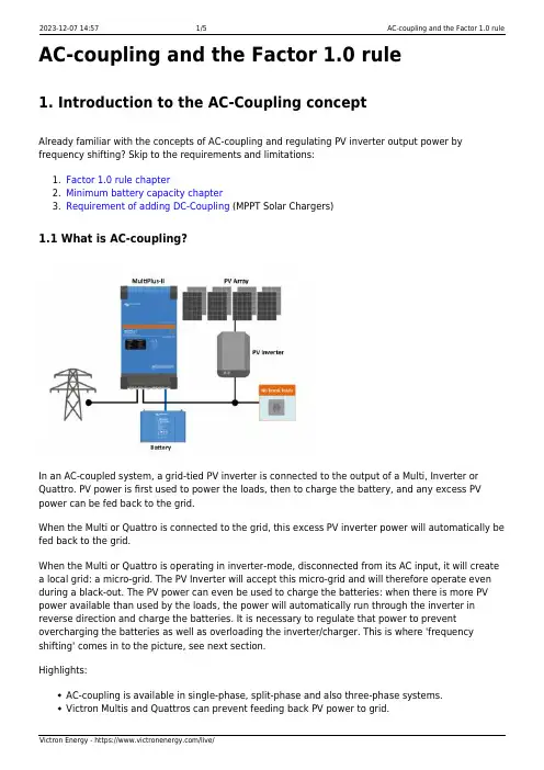
AC-coupling and the Factor 1.0 rule1. Introduction to the AC-Coupling conceptAlready familiar with the concepts of AC-coupling and regulating PV inverter output power by frequency shifting? Skip to the requirements and limitations:Factor 1.0 rule chapter1.2.Minimum battery capacity chapter3.Requirement of adding DC-Coupling (MPPT Solar Chargers)1.1 What is AC-coupling?In an AC-coupled system, a grid-tied PV inverter is connected to the output of a Multi, Inverter or Quattro. PV power is ﬁrst used to power the loads, then to charge the battery, and any excess PV power can be fed back to the grid.When the Multi or Quattro is connected to the grid, this excess PV inverter power will automatically be fed back to the grid.When the Multi or Quattro is operating in inverter-mode, disconnected from its AC input, it will create a local grid: a micro-grid. The PV Inverter will accept this micro-grid and will therefore operate even during a black-out. The PV power can even be used to charge the batteries: when there is more PV power available than used by the loads, the power will automatically run through the inverter in reverse direction and charge the batteries. It is necessary to regulate that power to prevent overcharging the batteries as well as overloading the inverter/charger. This is where 'frequency shifting' comes in to the picture, see next section.Highlights:AC-coupling is available in single-phase, split-phase and also three-phase systems.Victron Multis and Quattros can prevent feeding back PV power to grid.Systems with only a grid-tied PV inverter will fail when there is a grid black-out. A micro-grid system will continue to operate, and even keep using solar power.It is also possible to run a AC-coupled micro-grid on a generatorMost brands of PV inverters can be used for these systems, they need to be setup to support frequency shifting, often called the island-mode or micro-grid mode. For SolarEdge settings, see Integrating with SolarEdge, for Fronius settings, see AC-coupled PV with Fronius PV Inverters & for reading and controling ABB/Fimer inverters, see AC-coupled PV with ABB/Fimer PV Inverters.To read out SMA inverters, see AC-coupled PV with SMA PV Inverters.If power will be fed back into the grid an anti-islanding device may have to be added to thesystem, depending on local regulations.1.2 What is frequency shifting?Frequency shifting is used to regulate the output power of a Grid-tie PV Inverter, or Grid-tie Wind inverter, by changing the frequency of the AC. The MultiPlus (or Quattro) will automatically control the frequency to prevent over charging the battery. See also the chapter 'Example & background'.For how to conﬁgure, see chapter 4.2. The Factor 1.0 ruleThe max PV power must be equal or less than the VA rating of the inverter/charger2.1 Rule deﬁnitionIn both grid-connected and oﬀ-grid systems with PV inverters installed on the output of a Multi, Inverter or Quattro, there is a maximum of PV power that can be installed. This limit is called the factor 1.0 rule: 3.000 VA Multi >= 3.000 Wp installed solar power. So for a 8.000 VA Quattro the maximum is 8.000 Wp, for two paralleled 8000 VA Quattros the maximum is 16.000 Wp, etc.2.2 Example and backgroundTo understand the background, consider the following situation: the PV inverter is at full power, supplying a big load. The Multi is in inverter mode. Then, suddenly and at once, this load is switched oﬀ. At that moment the PV inverter will continue operating at full power until the AC frequency has been increased. Increasing this frequency will take a very short time, but during that time all power will be directed into the batteries as there is no other place for it to go. This causes the following: When batteries are (nearly) full, the battery voltage will spike, possibly causing the Multi toswitch oﬀ in DC over-voltage alarm.The same spike will cause the AC output voltage of the Multi to spike, as these two are directly related, and when the spike on the battery voltage is high and fast enough, the Multi can never regulate its PWMs down fast enough to prevent the spike on AC. This spike can damage the PV inverter, the Multi and also any connected loads and other equipment.Another problem is that the Multi starts charge current protection.In the best case it might switch the grid inverter oﬀ immediately by setting the AC frequency tothe disconnect frequency as conﬁgured in the assistant.It is no problem to overpower the grid inverter by installing more solar panels. Some people do this to increase the generated solar power in winter time or rainy weather. Refer to the PV Inverter datasheet to maximum allowed installed PV power. Two times the inverter nameplate rating or even more is not uncommon!2.3 Charge current limitAnother question frequently asked is how can this factor be 1.0? Since the charger inside a 3000 VA Multi is not 3000 VA but closer to 2000 VA? The explanation lies in the fact that it will regulate. In other words: when there is too much power coming in, causing the charge current to exceed the limit, it will increase the output frequency again and will keep regulating the AC output frequency to charge with the limit.An example, a 3000 VA Multi, with 3000 W of solar power coming out of a PV inverter: 1.When the Multi is connected to the grid, all 3000 W can be fed back to the grid through theMulti, no problem.2.In case the Multi is not connected to the grid, the 3000 Wp is more than the charger in a Multi 3000 VA can handle. The charger is around 2000 W. Therefore the grid inverter assistant will automatically increase the frequency to reduce the output of the grid inverter, to matchmaximum charge current.2.4 Should you look at the total PV array, or the PV inverter rating?The mentioned 3000 Wp and 8000 Wp is the Watt-peak which can be expected from the solar system. So for an oversized PV array, where the total Watt-peak installed PV panels exceeds the power of the PV Inverter, you take the Wp from the inverter. For example 7000 Wp of solar panels installed, with an 6000 Watt PV grid inverter, the ﬁgure to be used in the calculations is 6000 Wp.And for an undersized PV array, where the total Wp of installed PV panels is less than the installed PV grid inverter, you use the Wp from the PV panels in your calculation.3. Minimum battery capacityBesides the relation between installed PV Power and the inverter/charger VA rating, it is also important to have a suﬃciently sized battery. The minimum battery capacity depends on the type of battery, lead or lithium.Note that, besides the minimum battery capacity, the mentioned sizes are often also the most economical battery size. In case used for self-consumption purposes that is. In case the goal is to increase autonomy, of course installing a large battery increases the system autonomy in case of a grid failure.3.1 Lead batteries1 kWp installed PV power requires approximately 5kWh of lead acid battery:100 Ah at 48 Vdc200 Ah at 24 Vdc400 Ah at 12 VdcEach additional 1 kWp of AC PV will require an additional proportional 5 kWh increase in lead acid battery storage.3.2 Lithium batteries1,5 kWp installed AC PV power requires 4.8 kWh of battery storage:100 Ah at 48 Vdc200 Ah at 24 Vdc400 Ah at 12 VdcEach additional 1.5 kWp of AC PV will require an additional proportional 4.8 kWh increase in battery storage.4 Requirement of adding DC-Coupling - MPPT Solar Chargers Not required for Energy Storage Systems in Germany or other reliable grid situations.Required for oﬀgrid systems as well as backup systems that need to overcome extended grid failures. Reason: recover from deadlock situation of AC-Coupling only situation.There is no Factor 1.0 limit that applies for DC coupled PV through a Victron MPPT. Nor is there a speciﬁc minimum amount of battery storage capacity, though please follow battery manufacture speciﬁcations for maximum charge rates. A rule of thumb is C10 (10% of Ah capacity in A) for lead acid batteries, and C2 (50% of Ah capacity in A) for lithium batteries.5 Software conﬁgurationMultis and Quattros with factory settings will not shift the AC output frequency to regulate charge current. When setting up an AC Coupled system, install either the ESS Assistant (for grid-connected systems) or the PV Inverter Support Assistant (for oﬀ-grid systems).The Inverter RS will automatically shift frequency without any additional conﬁguration required when a surplus/back-feed of AC is detected on the AC-output.Other options, all deprecated, are:1.Self-consumption Hub-2 v3 assistantHub-4 Assistant in combination with the PV Inverter support Assistant 2.3.Use the Inverter period time settings on the Virtual switch tab. MonitoringSee Connecing a PV inverter section of the GX manual.DISQUSView the discussion thread.。

GSK ZJY series spindle servo motor user 说明书

In this manual, we have tried as much as possible to describe all the various matters about the spindle servo motor. However, we can not describe all the matters which must not be done or which can not be done because there are so many possibilities. Therefore, matters which are not especially described in this manual should be regarded as “impossible” or “forbidden”.The copyright of the user manual is owned by GSK CNC Equipment Co., Ltd (Hereinafter referred to as GSK).It is against the law for any organization or individual to reproduce this manual in any form without the permission of GSK and GSK reserves the right to investigate its law duty.User Manual GSK ZJY Series Spindle Servo MotorIIPREFACEDear user:It’s our honor that you select GSK ZJY serial spindle servo motor (Hereinafter referred to as the motor).For safety of the motor and the product and for the normal and effective running, please read the manual carefully before installing and using the product.SAFETY PRECAUTIONThe incorrect connection and operation may cause the accident, so before using and operating the motor, please read the manual carefully!1. The motor is installed with the photoelectric encoder, and it’s not allowed to hit themotor. And the user can’t disassemble the photoelectric encoder by himself;otherwise, once the encoder is damaged, it may cause the motor out of running!2. In the normal climate, measure the insulation resistance, which the motor winding isagainst with the case, by 1000V megameter, and the value should NOT be less than20 MΩ.3. The motor and the drive should be connected correctly based on the manual toguarantee the protective grounding stable and reliable.4. The motor can run with load only after the motor is free of noise and vibration duringrunning from zero speed to the maximum speed in the dry run mode.5. During the motor running, it’s not allowed to touch the motor shaft and case.6. Only the qualified person can adjust and maintain the motor.7. It is forbidden to move the motor by dragging the wire (cable), the motor shaft or theencoder.8. GSK does NOT take any responsibility for any change on the product by the user, andthe warranty bill becomes invalid.All specifications and designs are subject to change without notice.IIIUser Manual GSK ZJY Series Spindle Servo MotorIVRESPONSIBILITYResponsibility of the manufacturer——The manufacturer should be in charge of the design and the structure of the motor and its accessories.——The manufacturer should be responsible for the safety of the motor and its accessories.——The manufacturer should be in charge of the provided information and suggestion for the user.Responsibility of the end user——The user should be very familiar with the safety operation through learning the motor safety operation or participating in the training session.——The user should be responsible for the safety after adding, changing or modifying the original motor and its accessories by himself.——The user should be in charge of the danger resulted from the operation, adjusting, maintenance, installation and storage which are not complied with the manual regulation.The manual is kept by the end user .Thank you for your corporation during using GSK product.ContentⅠ PRODUCT CHARACTERISTICS (1)Ⅱ RUNNING CONDITIONS (1)ⅢMODELS of the MACHINE (2)Ⅳ MAIN TECHNICAL PARAMETERS and OVERALL DIMENSION of the MOTOR (3)Ⅴ MECHANICAL CHARACTERISTICS CURVE of the MOTOR (11)ⅥCONNECTION and INSTALLATION of the MOTOR (21)ⅦSTORAGE of the MOTOR (23)ⅧTRANSPORTATION of the MOTOR (23)Ⅸ WARRANTY (23)VUser Manual GSK ZJY Series Spindle Servo Motor VI1Ⅰ PRODUCT CHARACTERISTICSGSK ZJY spindle servo motor is a new type of three-phase inductive motor with highperformance and adopts insulation structure of F level, corona resistance enameled wire dedicated for the frequency conversion motor and the encoder with high speed andprecision, and the motor is researched, developed and manufactured by GSK. The product is with thecharacteristics of the compact structure, high rotation precision, low noise, high reliability and high capability with low cost, etc, which can widely satisfy the requirements of the CNC machine tool and the automation.Ⅱ RUNNING CONDITIONS2.1 The height above sea level should NOT exceed 1000m.2.2 The environment temperature should be in the range of -10℃ ~ +40℃. 2.3 The relative air humidity is ≤90% (without the condensation).2.4AC voltage value of steady state is :（0.9 ~1.1）multiplies AC rated voltage value .User Manual GSK ZJY Series Spindle Servo Motor2ⅢMODELS of the MACHINE Example: ZJY208A-5.5BH-B5A1LY1-LZJY 208 A - 5.5B H -B5A1L Y1(**) - L ⑴ ⑵ ⑶ ⑷ ⑸⑹⑺ ⑻⑼⑽⑾ ⑿SR.NO MEANING ⑴ The spindle servo motor ⑵ Motor width （182, 208, 265） ⑶ Design sequence number (None: Original A ，B ，C……：design sequence number) ⑷ Rated power （Unit: kW ） ⑸ Rated speed （T: 300 r/min, U: 450 r/min, V: 600 r/min, W: 750 r/min,A: 1000 r/min, B:1500 r/min, C: 2000 r/min, D: 2500 r/min, E: 3000 r/min ）⑹ Max. speed （F: 12000 r/min, H:10000 r/min, M:7000 r/min, L:4500 r/min ） ⑺ Structure installation type:（B5 flange installation, B3 footing installation, B35 flange footing installation ） ⑻ Encoder type （None: Incremental 1024 p/r, A: Incremental 2500p/r, A1: Incremental 4096 p/r, A2: Incremental 5000 p/r, A4: Absolute 17 bit, A8: Absolute 19 bit ）⑼ Look the terminal box position in view from the shaft end (None: on the top, R: on the right, L: on the left).⑽ Shaft end (None: Optic axis, Y1: with the standard key slot) ⑾ Customer special order numbers are bracketed in two capitals.⑿Power supply voltage (none: three-phase 380～440V, L: three-phase 220V)Note: ZJY182-3.7BM, ZJY208A-5.5BL and ZJY208A-7.5BL encoder types are only the incremental 1024 p/r.Product characteristics:Adopt the totally enclosed air cooling structure without the case, good shape and compactstructure.Employ the optimized electromagnetic design with the characters of the low noise, smoothrunning and high efficiency.Introduce the imported bearing in high precision, and the rotor reaches the high precisionwith the dynamic balance process, which can ensure the motor running stable and reliable with small vibration and low noise in the maximum rotational speed range.Adopt the enameled wire of corona resistance, the motor can be driven reliably at theambient temperature of -15℃～40 and ℃in the environment with the dust and oil mist. Employ the encoder at high speed and in high precision, and it can be incorporated into thedrive with high performance for controlling the speed and the position in high precision. The overload capacity is strong and the motor is reliably running at rated power of 30min150% or 5min 300%.The speed regulation range is wide and the maximum speed can reach 12000r/min. Impact resistance, long lifetime and high cost performance. Protection level: IP54（GB/T 4942.1—2006） Insulation grade: Grade F （GB 755—2008） Vibration grade: Grade B （GB 10068—2008）Ⅳ MAIN TECHNICAL PARAMETERS and OVERALL DIMENSION of the MOTOR4.1 Refer to list 1 about the main technical parameters of three-phase 380~440V spindle motor and its overall dimension.List 1SPECITEMZJY182-1.5BH ZJY182-2.2BH ZJY182-2.2CF ZJY182-3.7BHZJY182-3.7DF ZJY182-5.5CF ZJY182-7.5EH ZJY182-3.7BM ZJY208A-3.7WLRated power （kW ） 1.5 2.2 2.2 3.7 3.7 5.5 7.5 3.7 3.7 Adapted GS drive type GS3048Y GS3048Y GS3050Y GS3050Y GS3050Y GS3075Y GS3100Y GS3050Y GS3050YDrive power supply （V ） Three-phase AC 380～440V 50/60Hz Rated current（A ） 7.3 7.5 9 15.5 13 19 21 10.4 11.3 Rated frequency （Hz ） 50 50 69 50 87 70 100 50 25 Rated torque （N·m ） 9.5 14 10.5 24 14 26 24 24 47 30min power （kW ） 2.2 3.7 3.7 5.5 5.5 7.5 11 5.5 5.5 30min current（A ）9.3 11 14.6 19.6 19 25 30 14.8 16 30min torque （N·m ）14 24 17.7 35 21 37 35 35 70 Rated speed（r/min ） 1500 1500 2000 1500 2500 2000 3000 1500 750Constant power range （r/min ） 1500～8000 1500～80002000～100001500～8000 2500～100002000～100003000～90001500～5000 750～3000Max. speed （r/min ） 10000 10000 12000 10000 12000 12000 10000 7000 4500Moment of inertia （kg·m 2） 0.0056 0.00740.0056 0.0115 0.00740.0115 0.0115 0.00930.0309Weight （kg ） 27 32 27 43 32 43 43 3777Installation typeIM B5 or B35Cooling fanpower supply Three phase AC 380～440V 50/60Hz 37W 0.1A Threephase AC 380～440V50/60Hz 40W 0.14AA 182 182 182 182 182 182 182 182 208B 91 91 91 91 91 91 91 91 104C 126 126 126 126 126 126 126 126 160D 185 185 185 185 185 185 185 185 215E 60 60 60 60 60 60 60 60 80F 324 351 324 406 351 406 406 376 524G 198 225 198 280 225 280 280 250 395H150h7 150h7 150h7 150h7 150h7 150h7 150h7 150h7 180h7 I 12 12 12 12 12 12 12 12 14 J28h6 28h6 28h6 28h6 28h6 28h6 28h6 28h6 38h6 K 184 184 184 184 184 184 184 184 212L 93 93 93 93 93 93 93 93 106 N 156 156 156 156 156 156 156 156 180 P 32 32 32 32 32 32 32 32 40 Q 132 159 132 214 159 214 214 184 320 S 60 60 60 60 60 60 60 60 80 T 4 4 4 4 4 4 4 4 5 Overall dimen-sion(refer to figures) Z 12 12 12 12 12 12 12 12 12User Manual GSK ZJY Series Spindle Servo Motor4List 1 (Continued)SPECITEMZJY208A-2.2AM ZJY208A-3.7AM ZJY208A-5.5AM ZJY208A-2.2BH ZJY208A-3.7BH ZJY208A-5.5BH ZJY208A-7.5BH ZJY208A-3.7BM ZJY208A-5.5BMRated power （kW ） 2.2 3.7 5.5 2.2 3.7 5.5 7.5 3.7 5.5 Adapted GS drive type GS3048Y GS3050Y GS3075Y GS3048Y GS3050Y GS3075Y GS3100Y GS3050Y GS3050YDrive power supply （V ） Three phase AC 380～440V 50/60Hz Rated current（A ） 6.7 10.2 16.3 8.9 12.6 18.4 22.4 8.6 13 Ratedfrequency （Hz ） 33.3 33.3 33.3 50 50 50 50 50 50 Rated torque （N·m ） 21 35 53 14 24 35 48 24 35 30min power （kW ） 3.7 5.5 7.5 3.7 5.5 7.5 11 5.5 7.5 30min current（A ）10.6 14.2 20.5 13.8 18 24 32.2 12.7 16.9 30min torque （N·m ）37 53 72 24 35 48 70 35 48 Rated speed （r/min ） 1000 1000 1000 1500 1500 1500 1500 1500 1500 Constant power range （r/min ） 1000～4000 1000～4000 1000～4000 1500～8000 1500～8000 1500～8000 1500～8000 1500～5000 1500～5000Max. speed （r/min ） 7000 7000 7000 10000 10000 10000 10000 7000 7000Moment of inertia （kg·m 2）0.0168 0.0238 0.0309 0.0116 0.0168 0.0238 0.0309 0.0168 0.0238Weight （kg ） 51 66 77 49 51 66 77 51 66 Installation type IM B5 or B35 Cooling fanpower supplyThree phase AC 380～440V 50/60Hz 40W 0.14A A 208 208 208 208 208 208 208 208 208 B 104 104 104 104 104 104 104 104 104 C 160 160 160 160 160 160 160 160 160 D 215 215 215 215 215 215 215 215 215 E 60 80 80 60 60 80 80 60 80 F 414 469 524 364 414 469 524 414 469 G 285 340 395 235 285 340 395 285 340H180h7 180h7 180h7 180h7 180h7 180h7 180h7 180h7 180h7 I 14 14 14 14 14 14 14 14 14 J28h6 38h6 38h6 28h6 28h6 38h6 38h6 28h6 38h6 K 212 212 212 212 212 212 212 212 212L 106 106 106 106 106 106 106 106 106 N 180 180 180 180 180 180 180 180 180 P 40 40 40 40 40 40 40 40 40 Q 210 265 320 160 210 265 320 210 265 S 60 80 80 53 60 80 80 60 80 T 5 5 5 5 5 5 5 5 5 Overall dimen-sion(refer to figures) Z 12 12 12 12 12 12 12 12 12List 1 (Continued)SPECITEMZJY208A-7.5BM ZJY208A-5.5BL ZJY208A-7.5BL ZJY208A-11CM ZJY208A-11EHZJY265A-5.5WL ZJY265A-7.5WL ZJY265A-11WL ZJY265A-7.5AM ZJY265A-11AMRated power （kW ） 7.5 5.5 7.5 11 11 5.5 7.5 11 7.5 11 Adapted GS drive type GS3075Y GS3050Y GS3075Y GS3148Y GS3100Y GS3075Y GS3100Y GS3148Y GS3100Y GS3148YDrive power supply （V ） Three phase AC 380～440V 50/60Hz Rated current（A ） 17 12.9 17.9 28.3 25.2 16.3 21.4 30 21.5 30.9 Ratedfrequency （Hz ） 50 50 50 69 100 25 25 25 33.3 33.3 Rated torque （N·m ） 48 35 48 52.6 35 70 95.5 140 72 105 30min power （kW ） 11 7.5 11 15 15 7.5 11 15 11 15 30min current（A ）24.6 16.8 24 37 31.6 20.8 30.1 41 29 40.2 30min torque （N·m ）704870 71.6 48 95.5 140 191 105 145Rated speed （r/min ） 1500 1500 1500 2000 3000 750 750 750 1000 1000 Constant power range （r/min ） 1500～5000 1500～4500 1500～4500 2000～7000 3000～9000 750～3000750～3000750～30001000～4000 1000～4000Max. speed （r/min ） 7000 4500 4500 7000 100004500 4500 4500 7000 7000Moment of inertia （kg·m 2） 0.0309 0.0168 0.0238 0.03090.03090.07440.08260.086 0.04130.0826Weight （kg ）775266 77.8 66 107 125 143 89 125Installation type IM B5 or B35 IM B3 or B5Cooling fanpower supply Three phase AC 380～440V 50/60Hz 40W 0.14A Three phase AC 380～440V 50/60Hz 70W 0.21AA 208 208 208 208 208 265 265 265 265 265B 104 104 104 104 104 132 132 132 132 132C 160 160 160 160 160 185 185 185 185 185D 215 215 215 215 215 265 265 265 265 265E 80 80 80 110 80 110 110 110 110 110F 524 414 469 524 469 488 533 578 443 533G 395 285 340 395 340 347 392 437 302 392H180h7 180h7 180h7 180h7180h7230h7230h7230h7 230h7230h7I 14 14 14 14 14 14 14 14 14 14 J38h6 38h6 38h6 48h6 38h6 48h6 48h6 55h6 48h6 48h6 K 212 212 212 212 212 256 256 256 256 256L 106 106 106 106 106 135 135 135 135 135 N 180 180 180 180 180 230 230 230 230 230 P 40 40 40 40 40 40 40 40 40 40 Q 320 210 265 320 265 270 315 360 225 315 S 80 80 80 110 80 110 110 110 110 110 T 5 5 5 5 5 5 5 5 5 5 Overall dimen-sion(refer to figures) Z 12 12 12 12 12 15 15 15 15 15List 1 (continued)SPEC ITEMZJY265A-15AM ZJY265A-5.5BM ZJY265A-7.5BM ZJY265A-11BMZJY265A-15BMZJY265A-18.5BMZJY265A-22BM ZJY265A-7.5BH ZJY265A-11BHZJY265A-15BHRated power （kW ） 15 5.5 7.5 11 15 18.5 22 7.5 11 15 Adapted GS drive type GS3150Y GS3050Y GS3075Y GS3100Y GS3150Y GS3150Y GS3200Y GS3100Y GS3148Y GS3150YDrive power supply （V ） Three phase AC 380～440V 50/60Hz Rated current（A ） 48.3 15 18 26 35 48.7 58 21 30 40.7 Ratedfrequency （Hz ） 33.3 50 50 50 50 50 50 50 50 50 Rated torque （N·m ） 143 35 49 72 98 118 140 48 70 95 30min power （kW ） 18.5 7.5 11 15 18.5 22 30 11 15 18.5 30min current（A ）56 18.7 26 34 42 54.7 73 28.5 38.3 42.7 30min torque （N·m ）177 48 74 100 123 140 191 70 95 118 Rated speed （r/min ） 1000 1500 1500 1500 1500 1500 1500 1500 1500 1500 Constant power range （r/min ） 1000～4000 1500～5000 1500～5000 1500～5000 1500～5000 1500～5000 1500～5000 1500～8000 1500～8000 1500～8000 Max. speed （r/min ） 7000 7000 7000 7000 7000 7000 7000 10000 1000010000Moment of inertia （kg·m 2）0.086 0.0205 0.0413 0.07440.08260.086 0.102 0.0413 0.07440.0826Weight （kg ） 143 62 89 107 125 143 162 89 107 125 Installation type IM B3 or B5 Cooling fanpower supplyThree phase AC 380～440V 50/60Hz 70W 0.21A A 265 265 265 265 265 265 265 265 265 265 B 132 132 132 132 132 132 132 132 132 132 C 185 185 185 185 185 185 185 185 185 185 D 265 265 265 265 265 265 265 265 265 265 E 110 110 110 110 110 110 110 110 110 110 F 578 383 443 488 533 578 633 443 488 533 G 437 242 302 347 392 437 492 302 347 392H230h7 230h7 230h7 230h7230h7230h7230h7230h7 230h7230h7I 14 14 14 14 14 14 14 14 14 14 J48h6 48h6 48h6 48h6 48h6 55h6 55h6 48h6 48h6 48h6 K 256 256 256 256 256 256 256 256 256 256L 135 135 135 135 135 135 135 135 135 135 N 230 230 230 230 230 230 230 230 230 230 P 40 40 40 40 40 40 40 40 40 40 Q 360 165 225 270 315 360 415 225 270 315 S 110 110 110 110 110 110 110 110 110 110 T 5 5 5 5 5 5 5 5 5 5 Overall dimen-sion(refer to figures) Z 15 15 15 15 15 15 15 15 15 154.2 Refer to list 2 about the main technical parameters of three-phase 220V spindle motor and its overall dimension.List 2SPECITEMZJY182-1.5BH ZJY182-2.2BH ZJY182-2.2CFZJY182-3.7BH ZJY182-3.7DF ZJY182-5.5CF ZJY208A-3.7WL ZJY208A-2.2AMRated power （kW ） 1.5 2.2 2.2 3.7 3.7 5.5 3.7 2.2 Adapted GS drive type GS2050Y GS2050Y GS2075Y GS2100Y GS2100Y GS2100Y GS2075Y GS2050YDrive power supply （V ） Three phase AC 220V 50/60Hz Rated current（A ） 10.7 12.9 14.5 23.5 22.9 32.5 19.6 11.6 Ratedfrequency （Hz ） 50 50 69 50 87 70 25 33.3 Rated torque （N·m ） 9.5 14 10.5 24 14 26 47 21 30min power （kW ） 2.2 3.7 3.7 5.5 5.5 7.5 5.5 3.7 30min current（A ）17.6 20 23 36.4 33.8 47.6 27.3 18.4 30min torque （N·m ）14 24 17.7 35 21 37 70 37 Rated speed （r/min ） 1500 1500 2000 1500 2500 2000 750 1000 Constant power range （r/min ） 1500～8000 1500～80002000～100001500～80002500～100002000～10000750～30001000～4000 Max. speed （r/min ） 10000 10000 12000 10000 12000 12000 45007000Moment of inertia （kg·m 2）0.0056 0.0074 0.0056 0.0115 0.00740.0115 0.0309 0.0168Weight （kg ） 27 32 27 43 32 43 77 51 Installation type IM B5 or B35Cooling fanpower supply Three phase AC 220V 50/60Hz 37W 0.1A Three phase AC 220V 50/60Hz 40W 0.14AA 182 182 182 182 182 182 208 208B 91 91 91 91 91 91 104 104C 126 126 126 126 126 126 160 160D 185 185 185 185 185 185 215 215E 60 60 60 60 60 60 80 60F 324 351 324 406 351 406 524 414G 198 225 198 280 225 280 395 285H150h7 150h7 150h7 150h7 150h7 150h7 180h7 180h7 I 12 12 12 12 12 12 14 14 J28h6 28h6 28h6 28h6 28h6 28h6 38h6 28h6 K 184 184 184 184 184 184 212 212L 93 93 93 93 93 93 106 106 N 156 156 156 156 156 156 180 180 P 32 32 32 32 32 32 40 40 Q 132 159 132 214 159 214 320 210 S 60 60 60 60 60 60 80 60 T 4 4 4 4 4 4 5 5 Overall dimen-sion(refer to figures) Z 12 12 12 12 12 12 12 12List 2 (Continued)SPECITEMZJY208A-3.7AM ZJY208A-5.5AM ZJY208A-2.2BH ZJY208A-3.7BH ZJY208A-5.5BH ZJY208A-3.7BM ZJY208A-5.5BM ZJY208A-7.5BMRated power （kW ） 3.7 5.5 2.2 3.7 5.5 3.7 5.5 7.5 Adapted GS drive type GS2075Y GS2100Y GS2075Y GS2100Y GS2100Y GS2075Y GS2100Y GS2100YDrive power supply （V ） Three phase AC 220V 50/60Hz Rated current（A ） 17.7 28.2 15.3 21.8 31.8 14.9 22.5 29.4 Ratedfrequency （Hz ） 33.3 33.3 50 50 50 50 50 50 Rated torque （N·m ） 35 53 14 24 35 24 35 48 30min power （kW ） 5.5 7.5 3.7 5.5 7.5 5.5 7.5 11 30min current（A ）24.6 35.5 23.9 31.2 41.6 22 29.3 42.6 30min torque （N·m ）53 72 24 35 48 35 48 70 Rated speed （r/min ） 1000 1000 1500 1500 1500 1500 1500 1500 Constant power range （r/min ） 1000～4000 1000～4000 1500～8000 1500～8000 1500～8000 1500～5000 1500～5000 1500～5000Max. speed （r/min ） 7000 7000 10000 10000 10000 7000 7000 7000Moment of inertia （kg·m 2）0.0238 0.0309 0.0116 0.0168 0.0238 0.0168 0.0238 0.0309Weight （kg ） 66 77 49 51 66 51 66 77 Installation type IM B5 or B35 Cooling fanpower supplyThree phase AC 220V 50/60Hz 40W 0.14A A 208 208 208 208 208 208 208 208 B 104 104 104 104 104 104 104 104 C 160 160 160 160 160 160 160 160 D 215 215 215 215 215 215 215 215 E 80 80 60 60 80 60 80 80 F 469 524 364 414 469 414 469 524 G 340 395 235 285 340 285 340 395H180h7 180h7 180h7 180h7 180h7 180h7 180h7 180h7 I 14 14 14 14 14 14 14 14 J38h6 38h6 28h6 28h6 38h6 28h6 38h6 38h6 K 212 212 212 212 212 212 212 212L 106 106 106 106 106 106 106 106 N 180 180 180 180 180 180 180 180 P 40 40 40 40 40 40 40 40 Q 265 320 160 210 265 210 265 320 S 80 80 53 60 80 60 80 80 T 5 5 5 5 5 5 5 5 Overall dimen-sion(refer to figures) Z 12 12 12 12 12 12 12 124.3 About the outline drawings of the motors of various installation types please referto the following figures.Flange installation type（B5）Footing installation type (B3) and left & right outlet method Flange & footing installation type（B35）and left & right outlet method4.4 Dimension of the Standard Key Slot4.4.1 ZJY182-3.7BM, ZJY208A-3.7BM, ZJY208A-2.2AMThe configuration keys: GB/T 1096 Key: 8×7×50About the dimension of the shaft end key slot, refer to the following left figure; And the central screw hole dimension on the end face of the rotary axis is M10×20.4.4.2 ZJY208A-5.5BM, ZJY208A-7.5BM, ZJY208A-5.5BL, ZJY208A-7.5BL,ZJY208A-3.7AM, ZJY208A-3.7WL, ZJY208A-5.5AMThe configuration keys: GB/T 1096 Key: 10×8×70About the dimension of the shaft end key slot, refer to the following figure; and the central screw hole dimension on the end face of the rotary axis is M10×20.ZJY265A-11BM, ZJY265A-15BM, ZJY265A-7.5AM, ZJY265A-11AM,ZJY265A-15AM, ZJY208A-11CMThe configuration keys: GB/T 1096 Key: 14×9×90About the dimension of the shaft end key slot, refer to the following figure; and the central screw hole dimension on the end face of the rotary axis is M10×20.The configuration keys: GB/T 1096 Key: 16×10×90About the dimension of the shaft end key slot, refer to the following figure; and the central screw hole dimension on the end face of the rotary axis is M10×20.ⅤMECHANICAL CHARACTERISTICS CURVE of the MOTOR Figure:Power or torque in the continuous working state；Power or torque in 30min working state.Motor type Power curve Torque curveZJY182-1.5BH ZJY182-2.2BH ZJY182-2.2CF15002.210000115001.580001.552002.20.511.522.50500010000Speed (r/min)Power (kW)15001480001.7100000.915009.5520042468101214160500010000Speed (r/min)Torque (N·m)15003.7100001.515002.280002.237143.70.511.522.533.540500010000Speed(r/min)Power (kW)20003.720002.2120001100002.275003.70.511.522.533.540500010000Speed(r/min)Power (kW)150023.580002.6100001.415001437149.55101520250500010000Speed (r/min)Torque (N· m)200017.6100002.1120000.7200010.575004.751015200500010000Speed (r/min)Torque (N· m)Motor typePower curveTorque curveZJY182-3.7BHZJY182-3.7DFZJY182-5.5CFZJY182-7.5EH1500 5.5100002.215003.780003.756005.50 1 2 3 4 5 6 0500010000Speed (r/min)Power (kW)1500358000 4.4100002.1150023.55600 9.30510********35400500010000Speed (r/min)Torque (N· m)25005.525003.7120002.2100003.776005.50 1 2 3 4 5 6 0500010000Speed (r/min)Power (kW)250021100003.5120001.7250014.17600 6.95101520250500010000Speed (r/min)Torque (N·m)2000 7.5120003.720005.5100005.577777.50 1 2 3 4 5 6 7 8 0500010000Speed (r/min)Power (kW)200035.8100005.2120002.9200026.277779.20510********35400500010000Speed (r/min)Torque (N· m)30001130007.5100005.590007.57250110 2 4 6 8 10 12 0500010000Speed (r/min)Power (kW)3000353000 23.890007.9100005.27250 14.405101520253035400500010000Speed (r/min)Torque (N· m)Motor type Power curve Torque curveZJY182-3.7BM ZJY208A-3.7WL ZJY208A-2.2AM ZJY208A-3.7AM15005.570002.215003.750003.726005.51234560200040006000Speed (r/min)Power (kW)1500355000770003150023.5260020.25101520253035400200040006000Speed (r/min)Torque (N· m)7505.545002.27503.730003.712005.5123456020004000Speed (r/min)Power (kW)75070300011.745004.675047.1120043.71020304050607080020004000Speed (r/min)Torque (N· m)10003.770000.4510002.240002.214283.70.511.522.533.540200040006000Speed (r/min)Power (kW)100035.340005.270000.6100021142824.75101520253035400200040006000Speed (r/min)Torque (N· m)10005.570001.510003.740003.715455.51234560200040006000Speed (r/min)Power (kW)100052.540008.870002100035.3154533.91020304050600200040006000Speed (r/min)Torque (N· m)Motor typePower curveTorque curveZJY208A-5.5AMZJY208A-2.2BHZJY208A-3.7BHZJY208A-5.5BH1000 7.570003.210005.540005.513917.50 1 2 3 4 5 6 7 8 0200040006000Speed (r/min)Power (kW)100071.64000 13.170004.3100052.51391 51.40102030405060708002000 40006000Speed (r/min)Torque (N· m)15003.7100001.515002.280002.237143.70 0.5 1 1.5 2 2.5 3 3.5 4 0500010000Speed (r/min)Power (kW)150023.58000 2.6100001.41500143714 9.55101520250500010000Speed (r/min)Torque (N· m)1500 5.5100002.215003.780003.756005.50 1 2 3 4 5 6 0500010000Speed (r/min)Power (kW)1500358000 4.4100002.1150023.55600 9.30510********35400500010000Speed (r/min)Torque (N· m)1500 7.5100003.715005.580005.557777.50 1 2 3 4 5 6 7 8 0500010000Speed (r/min)Power (kW)150047.78000 6.5100003.51500355777 12.3010********600500010000Speed (r/min)Torque (N· m)Motor type Power curve Torque curveZJY208A-7.5BH ZJY208A-3.7BM ZJY208A-5.5BM ZJY208A-7.5BM150011100005.515007.580007.5450011246810120500010000Speed(r/min)Power (kW)15007080008.9100005.2150047.7450023.310203040506070800500010000Speed (r/min)Torque (N· m)15005.570002.215003.750003.726005.51234560200040006000Speed (r/min)Power (kW)1500355000770003150023.5260020.25101520253035400200040006000Speed (r/min)Torque (N· m)15007.570003.715005.550005.527777.5123456780200040006000Speed (r/min)Power (kW)150047.7500010.570005150035277725.71020304050600200040006000Speed (r/min)Torque (N· m)1500117000515007.550007.5220011246810120200040006000Speed (r/min)Power (kW)150070500014.370006.8150047.7220047.710203040506070800200040006000Speed (r/min)Torque (N· m)Motor typePower curveTorque curveZJY208A-5.5BLZJY208A-7.5BLZJY208A-11CMZJY208A-11EH15007.515005.545005.50 1 2 3 4 5 6 7 8 020004000Speed (r/min)Power (kW)1500 47.7150035450011.60102030405060020004000Speed (r/min)Torque (N· m)150********.545007.50 2 4 6 8 10 12 020004000Speed (r/min)Power (kW)1500701500 47.7450015.901020304050607080020004000Speed (r/min)Torque (N· m)2000152000117000110 2 4 6 8 10 12 14 16 0200040006000Speed (r/min)Power (kW)2000 71.62000 52.5700015010203040506070800200040006000Speed (r/min)Torque (N· m)300015300011100007.59000117857150 2 4 6 8 10 12 14 16 0500010000Speed (r/min)Power (kW)3000 47.7300035900011.6100007.1785718.21020304050600500010000Speed (r/min)Torque (N· m)。

comsol等离子体放电一维模型

3 |
ATMOSPHERIC PRESSURE CORONA DISCHARGE
Solved with COMSOL Multiphysics 5.1
The space charge density ρ is automatically computed based on the plasma chemistry specified in the model using the formula N ρ = q Z n – n k k e k = 1

For detailed information about electrostatics see Theory for the Electrostatics Interface in the Plasma Module User’s Guide.
1 |
ATMOSPHERIC PRESSURE CORONA DISCHARGE
Solved with COMSOL Multiphysics 5.1
cathode (-Vin)
simulated domain (1D)
anode
ri
ro
Figure 1: Not-to-scale cross section of the co-axial configuration. The negative potential (-Vin) is applied at the inner conductor (cathode) and the outer electrode is grounded (anode). The shaded area represents the ionization region created by the positive space charge distribution generated in the vicinity of the cathode.

杰克森（JEKSON）高频测试仪模型U9825、U9845、U9805X用户手册说明书

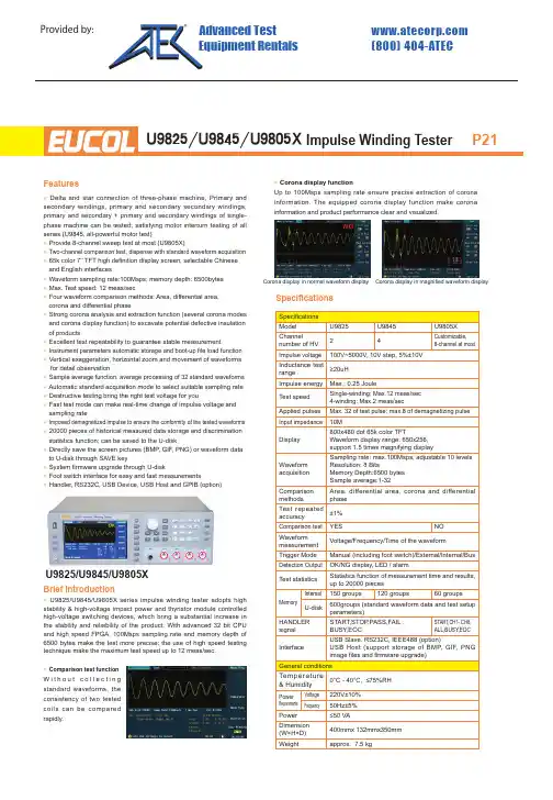
U9825/U9845/U9805X Impulse Winding Tester P21Features● Delta and star connection of three-phase machine, Primary and secondary windings, primary and secondary secondary windings, primary and secondary + primary and secondary windings of single-phase machine can be tested; satisfying motor interturn testing of all series (U9845, all-powerful motor test)● Provide 8-channel sweep test at most (U9805X)● Two-channel comparison test, dispense with standard waveform acquisition ● 65k color 7’’ TFT high definition display screen, selectable Chinese and English interfaces● Waveform sampling rate:100Msps; memory depth: 6500bytes ● Max. Test speed: 12 meas/sec● Four waveform comparison methods: Area, differential area, corona and differential phase● Strong corona analysis and extraction function (several corona modes and corona display function) to excavate potential defective insulation of products● Excellent test repeatability to guarantee stable measurement● Instrument parameters automatic storage and boot-up file load function ● Vertical exaggeration, horizontal zoom and movement of waveforms for detail observation● Sample average function, average processing of 32 standard waveforms ● Automatic standard acquisition mode to select suitable sampling rate ● Destructive testing bring the right test voltage for you● Fast test mode can make real-time change of impulse voltage and sampling rate● Imposed demagnetized impulse to ensure the conformity of the tested waveforms ● 20000 pieces of historical measured data storage and discrimination statistics function; can be saved to the U-disk● Directly save the screen pictures (BMP , GIF, PNG) or waveform data to U-disk through SAVE key● System firmware upgrade through U-disk● Foot switch interface for easy and fast measurements● Handler, RS232C, USB Device, USB Host and GPIB (option)Brief Introduction● U9825/U9845/U9805X series impulse winding tester adopts high stability & high-voltage impact power and thyristor module controlled high-voltage switching devices, which bring a substantial increase in the stability and reliability of the product.With advanced 32 bit CPU and high speed FPGA, 100Msps sampling rate and memory depth of 6500 bytes make the test more precise; the use of high speed testing technique make the maximum test speed up to 12 meas/sec. ● Comparison test function W i t h o u t c o l l e c t i n g standard waveforms,the consistency of two tested coils can be compared rapidly.● Corona display functionUp to 100Msps sampling rate ensure precise extraction of corona information. The equipped corona display function make corona information and product performance clear and visualized.Corona display in normal waveform display Corona display in magnified waveform displaySpecificationsU9825/U9845/U9805XProvided by: (800) 404-ATECAdvanced Test Equipment Rentals®。

持续性心房颤动“2C3L”策略联合Marshall静脉无水乙醇化学消融疗效随访

DOI：10.3969/j.issn.1007-5062.2021.06.001•临床论著•持续性心房颤动“2C3L”策略联合Marshall静脉无水乙醇化学消融疗效随访左嵩桑才华赖一炜薄小雯蒋晨曦汤日波龙德勇杜昕董建增马长生［摘要］目的：评价持续性心房颤动“2C3L”策略联合Marshall静脉无水乙醇化学消融(EIVOM)术后随访1年的疗效。

方法：纳入2019年5月至2019年12月期间，于北京安贞医院接受持续性心房颤动“2C3L”消融策略联合Marshall静脉无水乙醇化学消融方案的患者48例，观察术后12个月有无心房颤动(AF)/心动过速(AD)发作。

结果：纳入的48例患者平均年龄(61.4±10.4)岁，其中36例男性(75.0%),25例长程持续性心房颤动(52.1%)。

43例(89.6%)成功完成了EIVOM,未完成的5例全部因未发现Marshall静脉。

所有患者均实现肺静脉隔离，二尖瓣峡部线、左心房顶部线及三尖瓣峡部线阻滞。

经过12个月的随访,42例(87.5%)患者在接受单次消融治疗后(无抗心律失常药物)未发作AF/AT,6例复发患者中的4例在随访期间行再次消融。

经过“2C3L”联合EIVOM策略治疗后，单次/多次消融1年无心房颤动/房性心动过速生存率为85.4%及93.5%。

所有病例均无严重并发症发生。

结论：持续性心房颤动“2C3L”联合EIVOM策略安全、有效，并能使持续性心房颤动患者在术后1年保持较高的窦性律维持。

［关键词］持续性心房颤动;Marshall静脉;导管消融;复发［中图分类号］R54［文献标志码］A［文章编号］1007・5062(2021)06・523・06One-year follow-up analysis on"2C3L”approach plus ethanol infusion into the vein of Marshall forpersistent atrial fibrillation ZUO Song,SANG Caihua,LAI Yiwei,BO Xiaowen,JIANG Chenxi,TANG Ribo,LONG Deyong,DU Xin,DONG Jianzeng,MA Changsheng Department of Cardiology,Beijing AnzhenHospital,Capital Medical University,Beijing Institute of Heart,Lung and Blood Vessel Diseases,Beijing100029,China［Abstract］Objective:To summarize the experience on the catheter ablation of persistent atrial fibrillation using the“2C3L”strategy combined with ethanol infusion in the vein of Marshall(EIVOM)after one-year follow-up.Methods:48patients with persistent atrial fibrillation using"2C3L"strategy combined withEIVOM were enrolled in Beijing Anzhen Hospital from May2019to December2019.Observe the occurrence ofatrial fibrillation or atrial tachycardia after a12-month follow-up.Results:The average age of the enrolled48patients was(61.4±10.4)years,the male ratio was75.0,and long-term persistent atrial fibrillation accountedfor about52.1.Among them,43cases(89.6%)completed EIVOM,and the remaining5cases were all due tothe absence of vein of Marshall.All patients achieved pulmonary vein isolation,mitral valve isthmus line,leftatrial roofline,and tricuspid isthmus line block.After12months of follow-up,42patients(87.5%)received asingle ablation treatment(without antiarrhythmic drugs)without AF/AT,and4of the six relapsed patients underwent reoperation during the follow-up period.After"2C3L"combined with EIVOM strategy treatment,the1year survival rate without atrial fibrillation/tachycardia after single/multiple ablation was85.4%and93.5%.Conclusions:Persistent atrial fibrillation"2C3L"strategy combined with EIVOM strategy is effective and feasible.It can maintain a high sinus maintenance rate in patients with persistent atrial fibrillation after a12-monthfollow-up.No serious complications occurred in all cases.［Keywords］Persistent atrial fibrillation；Catheter ablation；Vein of Marshall；Recurrence基金项目：国家重点研发计划课题(2016YFC1301002,2016YFC0900901,2020YFC2004803)；国家自然科学基金(82000322)作者单位：100029首都医科大学附属北京安贞医院-北京市心肺血管疾病研究所心血管内科通信作者：马长生，主任医师，教授，博士生导师，研究方向：心脏电生理和心律失常。

Influence of interband interaction on Isotope Effect Exponent of MgB2 Superconductors

Influence of Interband Interaction on Isotope Effect Exponent of MgB2 Superconductors
P.Udomsamuthirun(1),C.Kumvongsa (2) ,A.Burakorn(1), P.Changkanarth(1)
2
1.Introduction The isotope effect exponent, α , is one of the most interesting properties of superconductors. In the conventional BCS theory α = 0 .5 for all element. In high- Tc superconductors , experimenter found that α is smaller than 0.5[1-3]. This unusual small value leads to suggestion that the pairing interaction might be predominantly of electronic origin with a possible small phononnic contribution[4]. To explain the unusual isotope effect in high- Tc superconductors, many models have been proposed such as the van Hove singularity[5-7], anharmonic phonon[8,9], pairing-breaking effect[10], and pseudogap[11,12]. The discovery of [13] of superconductivity in MgB2 with a high critical temperature , Tc ≈ 39 K, has attracted a lot of considerable attention. Various experiments [14-21] suggest the existence of mutiband in MgB2 superconductors.The gap values ∆( k ) cluster into two groups at low temperature, a small value of ≈ 2.5 meV and a large value of of ≈ 7 meV. The calculation of the electron structure [2226] support this conclusion. The Fermi surface consists of four sheets : two threedimensional sheets from the π bonding and antibonding bands ( 2p z ) , and two nearly cylindrical sheets from the two-dimensional σ band ( 2p x , y ) [24,27]. There is a large difference in the electron-phonon coupling on different Fermi surface sheet and this fact leads to multiband description of superconductivity. The average electronphonon coupling strength is found to be small values[14-16].Ummarino et al.[28] proposed that MgB2 is the weak coupling two band phononic system where the Coulomb pseudopotential and the interchannel paring mechanism are key terms to interpret the superconductivity state. Garland[29] has shown that Coulomb potential in the d-orbitals of transition metal reduce the isotope exponent whereas sp-metals generally shown a nearly full isotope effect. So for sp- metal as MgB2 , the Coulomb effect could not be account to explain the reduced of isotope exponent. Budko et al.[30] and Hinks et al.[31] measured the boron isotope exponent and estimated as α B = 0 . 26 ± 0 .03 and nearly zero magnesium isotope effect. The boron isotope exponent is closed to that obtained for the YNi2 B2 C and LuNi2 B2 C borocarbideds [32,33] where theoretical work[34] suggested that the phonons responsible for the superconductivity are high- frequency boron optical modes. This observation is consistent with a phonon- mediated BCS superconducting mechanism that boron phonon modes are playing an important role. The theory of thermodynamic and transport properties of MgB2 was made in the framework of the two band BCS model [35-43]. Zhitomirsky and Dao[44] derive the Ginzburg-Landau functional for two gap superconductors from the microscopic BCS model and then investigate the magnetic properties . The concept of multiband superconductors was first introduced by Suhl[45] and Moskalenke[46] in case of large disparity of the electron-phonon interaction for different Fermi-surface sheets. The purpose of this paper is to derive the exact formula of Tc ‘s equation and the isotope effect exponent of two-band superconductors in weak-coupling limit by considering the influence of interband interaction . The paring interaction in each band consisted of 2 parts : a attractive electron-phonon interaction and a attractive non-electron-phonon interaction are included in our model. 2. Model and calculation The properties of MgB2 suggest the two-band s-wave superconductors(σ-band and π -band). And in each band ,it may have two energy

整体立铣刀圆弧刃前刀面的磨削轨迹算法

机械设计与制造Machinery Design & Manufacture147第6期2021年6月整体立铳刀圆弧刃前刀面的磨削轨迹算法张潇然，罗斌，陈思远，程雪峰（西南交通大学机械工程学院，四川成都610031）摘要:针对圆弧立铳刀磨削中周齿前刀面与端齿前刀面的过渡问题，提出磨削圆弧刃前刀面的砂轮轨迹算法，以此实现周齿与端齿前刀面的光滑连接。

定义了一种切深磨削点轨迹曲线，可以同时约束圆弧前刀面的宽度和前角；定义了圆弧刃在平面中的瞬时前刀面，计算在瞬时前刀面中的砂轮磨削轨迹和姿态,再经过空间坐标变换，得出砂轮实际加工轨迹。

通过C++将算法编写为相应程序，进行仿真和实际加工验证，所得验证结果证明了该方法的正确性和可行性。

关键词:立铳刀;磨削加工;端齿圆弧刃；前刀面中图分类号:TH16;TH161 文献标识码:A 文章编号:1001-3997(2021)06-0147-03The Grinding Algorithm for the Rake Face of the Arc Edge of the Integral End MillZHANG Xiao-ran, LUO Bin, CHEN Si-yuan, CHENG Xue-feng(School of Mechanical Engineering , Southwest Jiaotong University, Sichuan Chengdu 610031, China)Abstract :A iming at the transition problem between the rake f ace of p eripheral f lank and the rake f ace of e nd tooth in the circulararc end mill, proposing a grinding algorithm f or the rake face of the arc edge that can achieve smooth connection between thetwo. Defines a depth-of-depth curve that can simultaneously constrain the width and rake angle of t he arc rake f ace. Defines theinstantaneous rake f ace of the arc edge and calculates the grinding path and attitude of t he grinding wheel in it. After the space coordinate transformation, the actual machining track of t he grinding wheel is obtained. Programming the algorithm into corre sponding p rogram by C++, and p erformming the simulation and p rocessing verification. The obtained results prove the correctnessand f easibility of t he algorithm.Key Words :End Mill ； Grinding ； Arc Edge ； Rake Face1引言圆弧头立铳刀是目前常见的高速切削刀具,具有制造成本低、材料切除率大等特点。

1、下载文档前请自行甄别文档内容的完整性，平台不提供额外的编辑、内容补充、找答案等附加服务。
2、"仅部分预览"的文档,不可在线预览部分如存在完整性等问题,可反馈申请退款(可完整预览的文档不适用该条件!)。
3、如文档侵犯您的权益，请联系客服反馈,我们会尽快为您处理(人工客服工作时间：9:00-18:30)。

–2– 1E1740.7-2942 show power law spectra extending up to hundreds of keV (e.g. Gilfanov et al. 1994; Tanaka & Levin 1995). The characteristic features of reﬂection have been seen in GBHC as well (e.g. Done et al. 1992). AGN and GBHC are believed to be powered by accretion through an accretion disk. In the uniﬁed model for AGN (e.g. Antonucci 1993), it is believed that we are viewing the disks in Seyfert 1 galaxies more or less face on, while for Seyfert 2 galaxies we are viewing the disk more or less edge on through a molecular torus. In GBHC sources we are viewing the binary system along some given (possibly time dependent) direction. The X-ray spectra indicate the existence of both hot X-ray emitting and cold reﬂecting gas components. The exact geometry is not known, but a currently popular model is the two-phase disk-corona model (e.g. Haardt & Maraschi 1991, 1993, hereafter HM93). The black body disk radiation from the cold disk (in the EUV for AGN, and in the soft X-rays for GBHC) enters the hot corona from one side and gets Comptonized into the X-rays. Part of this X-ray radiation is incident on the cold disk and is partly reﬂected but mainly reprocessed into soft black body radiation. The remaining part forms the X-ray spectrum leaving the disk-corona system. Both the black body and the Comptonized spectrum are anisotropic so observers at diﬀerent viewing angles see diﬀerent spectra (HM93). It immediately clear that such models are neither homogeneous nor spherically symmetric. In order to correctly interpret observed X-ray spectra of AGN and GBHC one needs to know the theoretical spectra for mildly relativistic temperature and for diﬀerent viewing angles. Theoretical Comptonized spectra have been computed for two decades now. Almost all work make simplifying assumptions that render them useless for interpreting X-ray spectra from sources were anisotropic eﬀects are important. We brieﬂy discuss standard methods for modeling Comptonized spectra from AGN and GBHC at mildly relativistic temperatures. One approach is to treat the photon and pair producing processes as well as the energy and pair balance in great detail, but to make large simpliﬁcations regarding the radiative transfer using various prescriptions for the spectral shape and using simple escape probabilities to get the photon density (e.g. Zdziarski 1985; Pietrini & Krolik 1995). Such calculations can only give very approximate relations between the typical spectral shape and other parameters. Other approaches are to do detailed radiative transfer using Monte Carlo methods for geometries such as slabs or spheres (e.g. Hua & Titarchuk 1995) or to improve the analytical theory of Comptonization (e.g. Titarchuk 1994). Normally the following simpliﬁcations are made: 1) processes other than Comptonization are neglected, 2) pair balance is not imposed, 3) angle dependence of output spectra is not considered, 4) the soft photon injection is homogeneous throughout the source. There are some exceptions. For example, Skibo et al. (1995) includes bremsstrahlung, pair production, and pair balance, and Zdziarski et al. (1994) assume the soft photons to be injected at one of the slab surfaces. Most work neglect reﬂection by cold matter. The few papers considering polarized radiative transfer (e.g. Sunyaev & Titarchuk 1985; Haardt & Matt 1993) use the Rayleigh matrix, which is not valid for temperatures and photon energies
Juri Poutanen and Roland Svensson Stockholm Observatory, S-133 36 Saltsj¨ obaden, Sweden; juri@astro.su.se, svensson@astro.su.se ABSTRACT We consider two phase accretion disk-corona models for active galactic nuclei and some X-ray binaries. We describe in detail how one can exactly solve the polarized radiative transfer and Comptonization using the iterative scattering method, while simultaneously solving the energy and pair balance equation for both the cold and hot phases. We take into account Compton scattering, photon-photon pair production, pair annihilation, bremsstrahlung, and double Compton scattering, as well as edisk. We consider coronae having slab geometry as well as coronae consisting of one or more well separated active regions of cylinder or hemisphere geometry. The method is useful for determining the spectral intensity and the polarization emerging in diﬀerent directions from disk-corona systems. The code is tested against a Monte-Carlo code. We also compare with earlier, less accurate, work. The method is more than an order of magnitude faster than applying Monte Carlo methods to the same problem and has the potential of being used in spectral ﬁtting software such as XSPEC.