On Finite Size Effects in $d=2$ Quantum Gravity
Quantum spin liquid emerging in 2D correlated Dirac fermions

英语翻译
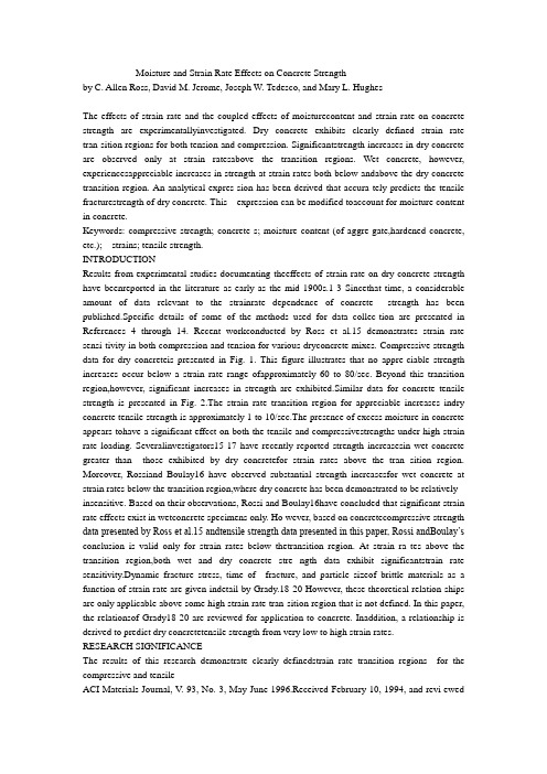
Moisture and Strain Rate Effects on Concrete Strengthby C. Allen Ross, David M. Jerome, Joseph W. Tedesco, and Mary L. HughesThe effects of strain rate and the coupled effects of moisturecontent and strain rate on concrete strength are experimentallyinvestigated. Dry concrete exhibits clearly defined strain rate tran-sition regions for both tension and compression. Significantstrength increases in dry concrete are observed only at strain ratesabove the transition regions. Wet concrete, however, experiencesappreciable increases in strength at strain rates both below andabove the dry concrete transition region. An analytical expres-sion has been derived that accura tely predicts the tensile fracturestrength of dry concrete. This expression can be modified toaccount for moisture content in concrete.Keywords: compressive strength; concrete s; moisture content (of aggre-gate,hardened concrete, etc.); strains; tensile strength.INTRODUCTIONResults from experimental studies documenting theeffects of strain rate on dry concrete strength have beenreported in the literature as early as the mid-1900s.1-3 Sincethat time, a considerable amount of data relevant to the strainrate dependence of concrete strength has been published.Specific details of some of the methods used for data collec-tion are presented in References 4 through 14. Recent workconducted by Ross et al.15 demonstrates strain rate sensi-tivity in both compression and tension for various dryconcrete mixes. Compressive strength data for dry concreteis presented in Fig. 1. This figure illustrates that no appre-ciable strength increases occur below a strain rate range ofapproximately 60 to 80/sec. Beyond this transition region,however, significant increases in strength are exhibited.Similar data for concrete tensile strength is presented in Fig. 2.The strain rate transition region for appreciable increases indry concrete tensile strength is approximately 1 to 10/sec.The presence of excess moisture in concrete appears tohave a significant effect on both the tensile and compressivestrengths under high strain rate loading. Severalinvestigators15-17 have recently reported strength increasesin wet concrete greater than those exhibited by dry concretefor strain rates above the tran sition region. Moreover, Rossiand Boulay16 have observed substantial strength increasesfor wet concrete at strain rates below the transition region,where dry concrete has been demonstrated to be relatively insensitive. Based on their observations, Rossi and Boulay16have concluded that significant strain rate effects exist in wetconcrete specimens only. Ho wever, based on concretecompressive strength data presented by Ross et al.15 andtensile strength data presented in this paper, Rossi andBoulay’s conclusion is valid only for strain rates below thetransition region. At strain ra tes above the transition region,both wet and dry concrete stre ngth data exhibit significantstrain rate sensitivity.Dynamic fracture stress, time of fracture, and particle sizeof brittle materials as a function of strain rate are given indetail by Grady.18-20 However, these theoretical relation-ships are only applicable above some high strain rate tran-sition region that is not defined. In this paper, the relationsof Grady18-20 are reviewed for application to concrete. Inaddition, a relationship is derived to predict dry concretetensile strength from very low to high strain rates.RESEARCH SIGNIFICANCEThe results of this research demonstrate clearly definedstrain rate transition regions for the compressive and tensileACI Materials Journal, V. 93, No. 3, May-June 1996.Received February 10, 1994, and revi ewedunder Institute publication policies.Copyright © 1996, American Concrete Institut e. All rights reserved, including the makingof copies unless permission is obtained fr om the copyright proprietors. Pertinentdiscussion will be published in the March-April 1997 ACI Materials Journal ifreceived by December 1, 1996.ACI member C. Allen Ross is a professor emeritus of aerospace engineering, mechan-ics, and engineering sciences, University of Florida, and a visiting professor at HQAir Force Civil Engineering Support Agen cy, Tyndall AFB, Florida. His researchinterests include the dynamic respon se of materials and structures.David M. Jerome is a senior research engineer in Wright Laboratory’s ArmamentDirectorate at Eglin AFB, Florida. He recently obtained his doctoral degree in engi-neering mechanics at the Univ ersity of Florida. His rese arch interests include thedynamic response of ma terials and structures.ACI member Joseph W. Tedesco is Gottlieb Professor of Civil Engineering, AuburnUniversity. His research interests include structural dynamics and finite element analysis.Mary L. Hughes is a research structural engineer in Wright Laboratory’s A ir BaseSurvivability Section at Tyndall AFB, Florida. She has received BS and MSdegrees in civil engineering.strengths of dry concrete. Below these transition regionsobserved strength increases are negligible; above thesetransition regions significant strength increases are exhib-ited. The moisture content of concrete has been shown tohave an important effect on strain rate sensitivity. Wetconcrete has displayed significant increases in strength atstrain rates below the dry conc rete transition region, and atstrain rates above the transitio n region, the strength increasesobserved in wet concrete are greater than those experiencedby dry concrete. This become s significant for submergedstructures when subjected to dynamic loadings that inducestrain rates above 1.0/sec. Finally, an analytical expression isderived from fracture mechanics theory that accuratelypredicts the tensile fracture strength of dry concrete over awide range of strain rates.Brittle fracture of concreteStudies on brittle fracture of condensed matter conductedby Grady18-20 are based on the assumption that local kineticenergy plus strain energy must exceed or equal the fracturesurface energy (all on a unit mass basis) for fracture to occur.Grady’s general assumption implies that at high st rain rates all of the particles of the same size must be fractured at thesame time. The basic premise is that peak stress σs is attainedin finite time ts at some strain rate and is given by(1)where B is bulk modulus, ε is strain, is strain rate, ρ isdensity, C0 is wave speed , ts is time to fracture, andσs is tensile fracture stress. At high strain rates, the fractureparticle diameter s is assumed to be limited by the wavespeed tos ≤ 2 C0ts(2)where the factor 2 comes from the assumption that a crackone-half length (s/2) = C0ts will be propagated in each directionfrom a fracture site.Details of the derivation of energy terms are presented inReferences 18 through 20 and are reviewed here. All energyterms are reckoned per unit mass andε·σsB ερC02ε·ts==ε·B ρ⁄ ()(3)(4)(5)where KIC is fracture toughness. Using the inequality KE + U ≥Γ(6)and Eq. (1) and (2), brittle fracture or spall strength σs, spallor fracture time ts, and fragment size s are found to beKinetic energy KE1120-------- - ρε·=2s2Strain energy density Uσs22 ρ C02--------------- =Fracture surface energy Γ 3 =KIC2ρC02s-------------- -(7)(8)(9)The strain energy density term of Eq. (6) has been shownto be approximately 15 times that of the kinetic energy term.Therefore, the kinetic energy term was neglected inobtaining Eq. (7) through (9).Eq.(7) through (9) are derived using the equality condition ofEq. (2) where the minimum particle size is limited by thewave speed. It has been shown experimentally15 that thecrack velocity of concrete is a function of strain rate. Thetheoretical limiting crack velocity is shown by Broek21 to be0.38 CL where CL is the longitudinal wave velocity. From Eq.(7) the slope of log10σs versuslog10εbecomes 1/3 . This slopeagrees reasonably well with the slope of regression curvesfitted to experimental data for concrete above a certain tran-sition strain rate.σs3 ρ C0KIC 2ε·() =13⁄ts1C0----- -3KICρCε·⁄()23⁄=s 2 =3KICρC0ε·⁄()23⁄However, Eq. (7) through (9) alone do not permit a contin-uous transition from low to high strain rates. Therefore, alow strain rate brittle fracture expression is introduced, usingcrack velocity as a function of strain rate, to facilitate thetransition from low to high strain rates.Low strain rate brittle fractureCrack velocity in concrete has been shown experimentallyto increase with strain rate15 (Fig. 3). Based on this data, therelation between crack velocity uc and strain rate ε.may bepresented as(10)where k is the intercept of the log10uc axis and m is the slopeof the linear plot of log10uc versus log10. Using Eq. (10),Eq. (2) may be rewritten as(11)tThe fracture toughness KIC that appears in Eq. (7) through(9) is assumed to be the static value and remains constantwith strain rate. Dynamic toughness KID, defined as thedynamic material resistance that is dependent on crackspeed, is given by Anderson22 as(12)where uc is crack velocity, ucl is limiting crack velocity, n isan experimentally determined value of approximately 1/ 3,and KIA is crack arrest toughness, defined in the limit as uc = 0,KID = KIAArrest toughness KIA appears to be approximately 25 to 50percent of KIC. The fracture toughness KIC of concrete isgiven by John and Shah23 as(13)where KIC is expressed in MPa-m1/ and fc′is the compressivestrength in MPa. The limiting velocity ucl has been shown tobe 0.38 CL by Broek21 and is assumed to approach Rayleighwave velocity CR as proposed by Anderson.22 Rayleigh velocity is approximately 0.6 CL for a Poisson’s ratio of ing Eq. (1), (10), (13), (3 ), (4), (5), and (6), anexpression for tensile fracture strength of concrete thatincorporates both crack velocity and fracture toughness asfunctions of strain rate is obtained. This fracture strength isgiven asKID KIA1 ucucl⁄ ()n–[] ⁄ ==ACI Materials Journal/May-June 1996(14)and is a function of strain rate, but most of the other param-eters are constants depending only on the compressive strength.Eq. (14) was evaluated using the following parameters:k = 100 (Reference 15)MPa (4060 and 8270 psi), were examined and the resultingstresses were normalized with respect to the stress at =10–5.7/sec, which yields the ratio of dynamic to static tensilestrength. The resulting curves are plotted versus log10 inFig. 2, along with experimental data. Very good correlationbetween Eq. (14) and the experimental concrete tensile datawas obtained. It is worth noting that very similar results wereobtained by Weerheijm25 using a much more elaborate and complicated derivation.It is important to point out th at a singularity occurs in thedenominator ofEq. (14) with the relationship of(15)–This singularity, which would limit the strain rate rangeover which Eq. (14) would be valid, can be overcome bylimiting the tensile strength to some peak value above thecritical strain rate given by(16)The advantage in using the ratio of dynamic to staticstrength, based on the low strain rate at which the static datawas obtained, is that the tensile strength at any strain rate isdetermined by simply multip lying the ordinate of thenormalized curve by the static tensile strength. This elimi-nates the necessity of having to know the arrest fracturetoughness of the concrete.As illustrated in Fig. 1, the compression data exhibits alow to high strain rate transitio n at a strain rate of approxi-mately 10 times that observed for the tensile data presentedin Fig. 2. This high strain rate compressive data was obtainedfrom experiments conducted on a 51-mm-diameter splitHopkinsonpressure bar (SHPB) using 51-mm-long specimensof the same diameter. (See ne xt section for a descriptionof the SHPB.) On failure these specimens experienced longi-tudinal cracking, thereby su ggesting transverse tensilefailure. Assuming the longitudinal cracking is the result ofstrain due to the Poisson effect, the transverse tensile strainεtt is computed byε·uclk⁄ ()1 m⁄=For a given Poisson’s ratio of 0.2 for concrete, both theaverage transverse tensile strain and strain rate are approxi-mately one-tenth of the compressive values. This results in acompressive transition strain rate that is 10 times the tensiletransition strain rate.Moisture and strain rate effectsIn an effort to experimentally determine the effects ofmoisture coupled with strain rate on concrete strength, aseries of wet/dry tests at low and high strain rates wereconducted. Tests were performed on completely wet, one-half dry, and dry concrete specimens.Concrete blocks of 0.3 x 0.3 x 0.3 m (12 x 12 x 12 in.) werecast, cured in air for 24 hr, placed in tap water for 7 to 10days, and then cored and cut to size underwater. The 51-mm-diameter, 51-mm-long (2.0 x 2.0-in.) specimens were storedin water for a total of 30 days.Previous tests15 have been completed to determine theoven time required for completely dry and one-half-dryspecimens. Oven drying at 230 F (110 C) with successivetimed weighings produced both the dry and one-half-dryspecimens. Wet specimens remained completely submergeduntil testing.Static tests were performed on all three types of specimensusing a closed-loop material test machine. Dynamic testswere accomplished using the Wright Laboratory SHPB atTyndall AFB, Florida. All tests specimens were 51 mm in diameter and 51-mm long. The split Hopkinson pressure baris a high strain rate device c onsisting of a gas gun, striker bar,incident bar, specimen, and transmitter bar, as shown inFig. 4(a). In general, the striker bar, propelled by the gasgun, impacts the incident bar and produces an elastic stresswave that propagates to the specimen, sandwiched betweenthe incident and transmitter bars. The elastic stress waveimpinges on the specimen wher e a portion of the stress waveis reflected back into the incident bar and a portion of thewave is transmitted into the transmitter bar. Strain gagesmounted on the incident and transmitter bar record the inci-dent and transmitted stress pulses. The integrated reflectedpulse is proportional to the strain in the specimen and thetransmitted pulse is proportional to the stress in the spec-imen. Using these pulses, a d ynamic stress-strain curve maybe formed. All specimens were 51 mm (2.0 in.) in diameter and 51-mm(2.0-in.) long. Specimens were cored from a solid blockusing a diamond core bit and cut to length by sawing, andends were ground flat. No capp ing material was used in thecompression tests. A steel metal bar, approximately 6.4-mmsquare and 51-mm long ( 0.25 x 0.25 x 2.0-in.), wasmachined to fit on each end of the splitting tensile specimen,as shown in Fig. 4(c).Standard compression tests were performed by applyingthe load along the longitudinal axis of the member [Fig. 4(b)],and splitting tensile tests were performed by rotating thespecimens 90 deg about a transverse specimen axis andapplying a load along a diametrical plane of the specimen, asshown in Fig. 4(c). The dynamic splitting tensile tests in theSHPB were first performed by Ross12 and numericallyanalyzed by Tedesco et al.26Results of wet/dry tests are presented in Fig. 5 and 6 fortension and compression, respectively. In both tension andcompression, the wet and one-half-dry data exhibit greaterstrength increases at higher strain rates than at lower strainrates. In both of these figures, the data is normalized withrespect to the static strength for each type of specimen. In allthe high strain rate work by the authors,8,12,13,15,26 all data isusually normalized with respect to data obtained at lowstrain rate (static test) using the same kind of specimens. Thisresults in the use of the dyna mic increase factor, defined asthe ratio of dynamic strength to static strength. Hopefully,byusing this one may eliminate problems such as differentmaturities relative to cure time and different mix strengths.Also, it is believed that effects of scale due to both specimensize and aggregate may also be minimized by the use of thedynamic increase factor.In all cases the static strengt h of the wet and one-half-dryspecimens was less than that of the static dry tests. However,in the dynamic test the strength of the wet and one-half-dryspecimens was generally greater than the strength of the dryspecimens. The strengths of all the tensile specimens testedare shown as a function of strain rate in Fig. 7.In observing the failure mechanisms of the various tests,one generally finds that in all tensile tests the appearance ofthe fractured surface is the same. The majority of the aggregatesare not fractured but pulled free from the paste. This holdstrue even when comparing dry, one-half-dry, and wet speci-mens to each other as well as for low and high strain ratetests. For compression tests, as the strain rate increases, thenumber of fractured pieces increases and the size of the frac-tured pieces decreases. Fractured surfaces of low strain rate compression specimens are similar to those of the tensilespecimens, but at the higher ra tes, the aggregates begin toshow multiple fractures.Static strength decreases in wet concrete as compared todry concrete have been attributed to the presence of moistureforcing the gel particles apart and reducing the van der Waalsforces.27 These reduced forces are proportional to thespecific surface energy; the criti cal stress for crack formationis then reduced and the overa ll specimen strength is reduced.This explanation appears plausible at low strain rates wherethe crack has time to seek the pa th of least resistance throughthe gel and gel matrix-aggregate interfaces. However, at highstrain rates the presence of the water appears to enhanceconcrete strength. Weerheijm25 attributes the increase of dryconcrete tensile strength at hi gh strain rates to effects ofinertia. The maximum rate at which concrete can fracture islimited, and any effort to force the crack to form at a higherrate simply results in increa sed deformation and strength.The presence of moisture in concrete has a tendency toamplify the inertia effects of the wet specimens, resulting ina strength greater than the dry strength.In addition, the presence of the moisture may also increasematerial stiffness and thereby afford better coupling forwave propagation. The increased stiffness with moisture present is evidenced by the hi gher modulus obtained for wetspecimens, as reported in Re ference 17. Also, the increasedstiffness of wet concrete at hi gh strain rates should result ina higher fracture toughness. A higher fracture toughnessused in Eq. (13) would predict a higher strength for thwet concrete.CONCLUSIONSDry concrete strength is relatively strain rate insensitivebelow the transition strain rates. These transition strain ratesare between 1 and 10/sec for tension, and between 60 and80/sec for compression. Wet co ncrete, however, exhibitssignificant increases in strength at strain rates below as wellas above the transition strain rates for dry concrete. Ananalytical expression that incorporates both crack velocityand fracture toughness as functions of strain rate has beenderived that accurately predicts the tensile fracture strengthof dry concrete. ACKNOWLEDGMENTSThe experimental work for this study was conducted at Wright Laborato-ry Air Base Survivability Section, Tyndall AFB, Florida.REFERENCES1. Watstein, D., “Effect of Straining Rate on the Compressive Strengthand Elastic Properties of Concrete,” ACI J OURNAL, Proceedings V. 24,No. 4, Apr. 1953, pp. 729-744.2. Goldsmith, W.; Kenner, V. H.; and Ricketts, T. E., “DynamicBehavior of Concrete,” Experimental Mechanics, V. 66, 1966, pp. 65-69.3. Melling er, F. M., and Birkimer, D. L., “Measurements of Stress andStrain on Cylindrical Test Specimens of Rock and Concrete under Impact Loading,” Te ch n i c a l R e p o r t 4-46, Department of Army Ohio River Divi- sion Laboratory, Apr. 1966.4. Green, H., “Impact Strength of Concrete,” Institution of Civil Engi-neers, Proceedings, V. 28, 1968, pp. 731-40.5. Hughes, B. P., and Gregory, R., “Impact Strength of Concrete UsingGreen's Ballistic Pendulum,” Institution of Civil Engineers, Proceedings,V. 81, 1968, pp. 731-40.6. Hughes, B. P., and Gregory, R., “Concrete Subjected to High Rates ofLoading in Compression,” Magazine of Concrete Research, V. 24, 1972,pp. 25-36.7. Hughes, B. P., and Watson, A. J., “Compressive Strength and Ulti-mate Strain of C oncrete under Impact Loading,” Magazine of ConcreteResearch , V. 30, 1978, pp. 189-99.8. Malvern, L. E., and Ross, C. A., “Dynamic Response of Concrete andConcrete Structures,” two annual re ports and a final report for AFOSRContract F49620-83-K007, University of Florida, Gainesville, Feb. 1984,Feb. 1985, and May 1986.9. Kormeling, H. A.; Zielinski, A. J.; and Reinhardt, H. W., “Experi-ments on Concrete under Single and Repeated Uniaxial Impact Tensile Loading,” Stevin Laboratory Report 5-80-3, Delft University of Tech-nology, 2nd Printing, 1981.10. Gran, J. K.; Florence, A. L.; and Colton, J. D., “Dynamic TriaxialTests of High-Strength Concrete,” Journal of Engineering Mechanics ,V. 115, 1989, pp. 891-904.11. Suaris, W., and Shah, S. P., “P roperties of Concrete Subjected toImpact Loading,” Journal of Structural Engineering , American Society ofCivil Engineers, V. 109, No. 7, 1983, pp. 1727-1741.12. Ross, C. Engineering and Services Laboratory, Air Force Engineering and Services Center, Tyndall AFB, Florida, 1989.13. Ross, C. A.; Kuennen, S. T.; and Tedesco, J. W., “Experimental andNumerical Analysis of High Strain Rate Concrete Tensile Tests,” Micro- mechanics of Failure of Quasibrittle Materials , S. P. Shah et al., eds.,Elsevier Applied Science, London, 1990, pp. 353-364.14. Sierakowski, R. L., “Dynamic Effects in Concrete Materials,”Application of Fracture Mechan ics to Cementitious Composites , S. P.Shah, ed., Martinus Nijhoff Publishi ng, Dordrecht, Netherlands, 1985.15. Ross, C. A.; Tedesco, J. W.; and Kuennen, S. T., “Effects of StrainRate on Concrete Strength,” ACI Materials Journal, V. 92, No. 1, Jan.-Feb. 1995, pp. 37-47.16. Rossi, P., and Boulay, C., “Etude experimentale du couplagefissuration-viscoité au se in du béton,” Project No. 9, Rapport GRECO, Rheologie des Géomatériaux,1989.17. Reinhardt, H. W.; Rossi, P.; a nd van Mier, J. G. M., “Joint Inves- tigation of Concrete at High Rates of Loading,” Materials and Structures, 23, 1990, pp. 213-216.18. Grad y, E. E., and Lipkin, J., “Criteria for Impulsive Rock Fracture,”Geophysical Research Letters, V. 7, No. 4, Apr. 1980, pp. 255-258.19. Grady, D. E., “Mechanics of Fracture under High Rate Stress Loading,” Sandia National Laboratories Report SAND 82-1148C, 1983. 20. Grady, D. E., and Lipkin, J ., “Mechanisms of Dynamic Fragmen- tation: Factors Governing Fragment Size,” Sandia National Laboratories Report SAND 84-2304C, 1984.21. Broek, D., Elementary Engineering Fracture Mechanics, M. Nijhoff Publishing, Boston, 1982.22. Anderson, T. L., Fracture Mechanics: Fundamentals and Applica-tions , CRC Press, Boca Raton, Florida, 1991.23. John, R., and Shah, S. P., “Effect of High Strain Rate of Loading on Fracture Parameters of Concrete,” Proceedings of Fra cture of Concreteand Rock , Society for Experimental M echanics-Réunion Internationaledes Laboratoires d'Essais et de Recherches sur les Matérieux et les Constructions International Conference, S. P. Shah and S. E. Swartz, eds., Society of Experimental Mechanics, Bethel, Connecticut, 1987, pp. 35-52. 24. Neville, A. M., Properties of Concrete, J. Wiley & Sons, New York, 1973, pp. 313-320.25. Weerheijm, J., “Concrete under Im pact Tensile Loading and Lateral Compression,” PhD dissertation, Delf t Univers ity of Technology, Delft, Netherlands, 1992.26. Tedesco, J. W.; Ross, C. A.; and Brunair, R. M., “Numerical Anal-ysis of Dynamic Split Cylinder Tests,” Computers and Structures, V.32, No. 3-4, 1989, pp. 609-624.27. Wittmann, F. H., “Interaction of Har dened Cement Paste and Water,” Journal of the American Ceramic Society , V. 56, No. 8, Aug. 1972, pp. 409-415.28. John, R., and Shah, S. P., “Fracture of Concrete Subjected to Impact Loading,” Cement, Concrete and Aggregates , CCAGDP V. 8, No. 1, 1986, pp. 24-32. A., “Split-Hopkinson Pressure Bar Tests,” ESL-TR-88-82,。
effect size公式
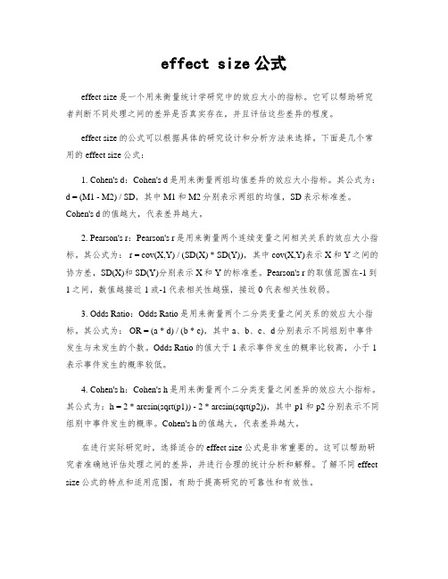
effect size公式effect size是一个用来衡量统计学研究中的效应大小的指标。
它可以帮助研究者判断不同处理之间的差异是否真实存在,并且评估这些差异的程度。
effect size的公式可以根据具体的研究设计和分析方法来选择。
下面是几个常用的effect size公式:1. Cohen's d:Cohen's d是用来衡量两组均值差异的效应大小指标。
其公式为:d = (M1 - M2) / SD,其中M1和M2分别表示两组的均值,SD表示标准差。
Cohen's d的值越大,代表差异越大。
2. Pearson's r:Pearson's r是用来衡量两个连续变量之间相关关系的效应大小指标。
其公式为: r = cov(X,Y) / (SD(X) * SD(Y)),其中cov(X,Y)表示X和Y之间的协方差,SD(X)和SD(Y)分别表示X和Y的标准差。
Pearson's r的取值范围在-1到1之间,数值越接近1或-1代表相关性越强,接近0代表相关性较弱。
3. Odds Ratio:Odds Ratio是用来衡量两个二分类变量之间关系的效应大小指标。
其公式为: OR = (a * d) / (b * c),其中a、b、c、d分别表示不同组别中事件发生与未发生的个数。
Odds Ratio的值大于1表示事件发生的概率比较高,小于1表示事件发生的概率较低。
4. Cohen's h:Cohen's h是用来衡量两个二分类变量之间差异的效应大小指标。
其公式为:h = 2 * arcsin(sqrt(p1)) - 2 * arcsin(sqrt(p2)),其中p1和p2分别表示不同组别中事件发生的概率。
Cohen's h的值越大,代表差异越大。
在进行实际研究时,选择适合的effect size公式是非常重要的。
这可以帮助研究者准确地评估处理之间的差异,并进行合理的统计分析和解释。
Large area single-mode parity–time-symmetric
OPTICS LETTERS / Vol. 37, No. 5 / March 1, 2012
Large area single-mode parity–time-symmetric laser amplifiers
Mohammad-Ali Miri,* Patrik LiKamWa, and Demetrios N. Christodoulides
CREOL, College of Optics and Photonics, University of Central Florida, Orlando, Florida 32816–2700, USA *Corresponding author: miri@ Received October 26, 2011; revised January 9, 2012; accepted January 15, 2012; posted January 17, 2012 (Doc. ID 157003); published February 17, 2012
By exploiting recent developments associated with parity–time (PT) symmetry in optics, we here propose a new avenue in realizing single-mode large area laser amplifiers. This can be accomplisБайду номын сангаасed by utilizing the abrupt symmetry breaking transition that allows the fundamental mode to experience gain while keeping all the higher order modes neutral. Such PT-symmetric structures can be realized by judiciously coupling two multimode waveguides, one exhibiting gain while the other exhibits an equal amount of loss. Pertinent examples are provided for both semiconductor and fiber laser amplifiers. © 2012 Optical Society of America OCIS codes: 140.3570, 140.4480, 130.2790.
SIZE-DEPENDENT EFFECTS IN PROPERTIES OF

© 2009 Advanced Study Center Co. Ltd.Corresponding author: R.A. Andrievski, e-mail: ara@icp.ac.ruSIZE-DEPENDENT EFFECTS IN PROPERTIES OFNANOSTRUCTURED MATERIALSR.A. AndrievskiInstitute of Problems of Chemical Physics, Russian Academy of Sciences, Chernogolovka, Moscow Region,142432, Russia Received: February 17, 2009Abstract. Size-dependent effects in nanostructured (nanocrystalline, nanophase or nanocomposite)materials are of great importance both for fundamental considerations and modern technology.The effect of the nanoparticle/nanocrystallite size on surface energy, melting point, phase transfor-mations, and phase equilibriums is considered as applied to nanostructured materials. The role of size-dependent effects in phonon, electronic, superconducting, magnetic, and partly mechanical properties is also analyzed in detail. Special attention is paid to the contribution of other factors such as the grain boundary segregations, interface structure, residual stresses and pores, non-uniform distribution of grain sizes, and so on. The little explored and unresolved problems are pointed and discussed.1. INTRODUCTIONSize-dependent effects (SDE, i.e. the characteris-tic size influence of grains, particles, phase inclu-sions, pores, etc ., on the properties of materials and substances) have been studied in physics,chemistry, and materials science for a long time. It is quite enough to list the following well-known equations of Laplace, Thomson (Kelvin), Gibbs-Ostwald, Tolman, J. Thomson, Hall-Petch,Nabarro-Herring, and Coble, which connect the capillary pressure (P ), saturated vapor pressure (p ), saturated solubility (C ), surface energy of flat surface (σ0), conductivity (λ), hardness (H ) and creep rate (′ε) correspondingly with the pore/in-clusion radius (r ), thickness film (h ) and grains/crys-tallites size (L ):P r =20σ/, (1)p r p rRT =B =B =002exp /,σΩ (2)C r C rRT =B =B=002exp /,σΩ (3)σσξ0012r r =B =B =+//,(4)λλh f =B =B =+0510./. (5)H L H AL =B =+−005., (6)~/,ε1L m (7)where p o is the equilibrium pressure of saturated vapor on flat surface, C o is the equilibrium solubil-ity of subject with flat surface, Ω is an atomic (mo-lar) volume, R is the gas constant, T is tempera-ture, ξ is the Tolman constant, λo is conductivity of grain-coarse material (thick film), f = h /l o , l o is the mean free pass of carriers (f < 1), H o is the friction stress in the absence of grain boundaries (GB) and A is a constant. The factors m =2 and 3 correspond to the Nabarro-Herring diffusion creep and to theCoble diffusion creep correspondingly.The development of modern advancednanostructured materials (NM) manifests some new problems such as the identification adaptabil-ity of these equations (1-7) and other those in na-108R.A. Andrievskinometer interval; the role of quantum effects as well as an influence of other factors in the NM prop-erties or their stability and reproducibility. All these things are very important and actual to consider the SDE features taking in mind the update high rate in this field and not only fundamental consid-erations, but the strategy optimal development for nanotechnology. These questions have been ana-lyzed early by the present author [1-5] and other investigators (see, e.g., [6-19]). It seems to be nec-essary to tell apart the SDE in the isolated nanosubjects (clusters, nanoparticles, nanowires,and nanotubes) and consolidated ones (nanobulks,nanocomposites, and nanofilms/nanocoatings).Analyses of SDE in consolidated NM can be found in reviews [1-6], but the most publications were devoted to nanoparticles and clusters. Naturally,the SDE topic as a whole seems not to be cov-ered, because there are many new results scat-tered throughout the literature.Taking into account the comprehensive books [9,10,13,15,16], this review is mainly devoted to the SDE recent analysis in consolidated NM (papers mainly from 2001-2002), although some results for isolated nanosubjects will be also considered with the exception of catalytic and biological properties.Moreover, the comprehensive problem on the SDE in mechanical properties will be also discussed in limited scale as applied only to brittle high-melting point compounds (see Section 4 below).It is important to point that there are at least five principal features of size effects in consolidated NM [1-5]:- the crystalline size reduction to the nanometer scale results in a significant increase of the role of the interface defects such as GB, triple junc-tions (TJ), and elastically distorted layers;- interfacial properties on a nanometer scale can be different from those of conventional grain-coarse materials;- the reduced crystallite size can be overlapped by characteristic physical lengths such as the mean free path of carriers or the Frank-Read loop size for dislocations and so on;- size effects in NM can have quantum nature if the crystallite size is commensurable with the De Broyle wavelength l B =D /(2m *E )1/2 where D is the Planck constant, m * is the electron effective mass, E is the electron energy. Based on known values of m * and E, it is possible to predict that the quantum size effects can be exhibited in met-als only when the crystallite size is lower than ~ 1nm. For semiconductors (especially with narrow gap-zone, e.g., InSb) and semimetals (e.g., Bi),the l B value is significantly higher and can be of about 100 nm;- unlike conventional grain-coarse materials, in NM there are many factors for masking SDE such as residual stresses, pores, TJ and the presence of other defects, progressive accumulation of inter-face segregations, non-equilibrium phase ap-pearance, and so on.All these peculiarities may reveal in the pres-ence of certain specific points in the size depen-dencies and in the non-monotonous change of the properties determined by decreasing of the grain size. As a rule, such non-monotonous change is especially characteristic for structure-sensitive properties. For example, such specific features, i.e.twist points, and non-monotonous change of prop-erties have been revealed in the known hardness and magnetic coercivity studies (see, e.g., [1,2,4]).Such changes can be connected with different fac-tors such as other mechanisms of SDE, progres-sive accumulation of segregations on interfaces,and so on.2. THERMODYNAMIC PROPERTIES 2.1. Surface energyThe problem concerning surface energy is impor-tant both for fundamental sense and for many materials science and engineering applications such as the prognosis of phase diagrams, the es-timations of the fracture, milling, dilution, wetting,nucleation, coagulation, recrystallization charac-teristics, and so on. In this connection, the reveal-ing of surface energy change in nanometer inter-val is of special interest.Tolman’s equation (4), i.e. the effect of the drop radius on surface energy, has been widely dis-cussed (see, e.g., [7,8,11,14,20-23]). Omitting the details of these calculations, which are based on different physical and chemical approaches, let us to consider these results as a whole. Being ap-plied to isolated nanocrystals under calculations [11,14], the amendment g (r ) to the conventional σ0value fixed on the capillary pressure (1) is describedby the following expressiong r r r rr rB=B =B =−+−−211422182ln /ln /For many nanocrystals this amendment is very small and comes into particular prominence (about 10%) only at r < 5 nm.The radius effect on surface energy can be also described by equations:109Size-dependent effects in properties of nanostructured materialsσσr Kr at r r at r r =B =<>456,,, (9)where K is a constant, r o is critical radius (of 2-10nm) [21]. There are other theoretical calculations that have revealed about the similar values of criti-cal radius lower of which surface energy is de-creased (see, e.g., [20,22]). The experimental re-sults in this field are very limited, ambiguous, and often mutually contradictory. From one side, elec-trochemical measurements have revealed the σr values about 0.2 J/m 2 and 0.7 J/m 2 for Ag nanoparticles of r ~ 50 nm and r ~ 150 nm accord-ingly to [24]. These values seem to be not so pre-cise but are reasonable (it is appropriate to com-pare them with the value of σo = 1.14 J/m 2 and with the GB energy of ~0.27 J/m 2). From the other side,the experimental study of size-dependent evapo-ration of free-spherical Ag and PbS nanoparticles using relationship (2) results in values of 7.2 J/m 2and 2.45 J/m 2 respectively, these values are sig-nificantly higher as compared to that of the flat bulks [25]. May be, this is an effect of the evaporation conditions (see Section 2.2) or there is a system-atic error in the experimental results [25].As applied to nanocrystalline solids the analy-sis of size- or curvature-dependent interface, free energy results to the following relationshipσσr t r =B =B≈−01/, (10)where t is an interfacial layer (the semi-width of GB in consolidated nanometals) [7,8]. It is easy to see that at the reasonable values of 2t ~ 1nm and r = 5 nm the σ decreasing is of 10% that is in close agreement with estimations under Eq. (8).In Debye approximation, the Tolman constant ξin Eq. (4) can be expressed asξα=′−151.,h =B(11)where h ’ is the height of atomic monolayer, α is the ratio of root-mean-square amplitude of thermal vi-brations of atoms on surface and in volume [23]. If α > 1 and ξ > 0, then σr < σo and in the opposite case α < 1 and ξ < 0 then σr > σo . As it will be seen from here on, these two cases are important as applied to the behavior analysis of nanoparticles in matrices.It is known that distinct feature of nanostructure in NM is that, with the grain size confinement, the part of TJ is increased and, accordingly, the part of GB is decreased (see, e.g., [4]). The computer modeling with account of GB and TJ contributions reveals that Ni grain size reducing is accompaniedby decrease of the total excess enthalpy (i.e. the total GB energy) [26]; this result quantitatively agrees with experimental data for nano Se [27].The calculated interface GB energy in Cu-Ni bilayered nanofilm changes from 0.9 J/m 2 to about 0.7 J/m 2 when bilayer thickness decreases from ~1 nm to ~0.4 nm [28].From the foregoing data it has been evident that in spite of different theoretical approaches in cal-culations, they are evidence of the σ decrease in the confinement of isolated nanosubjects and nanostructures in NM. It seems to be reasonable to introduce the amendments into grain/crystalline boundary energy values at L lower than near 10nm. However, it is also evident that experimental studies in this field are necessary for further de-tailed continuation.The comprehensive description of the SDE role in the other surface phenomena such as wetting,nucleation, adsorption, and capillarity can be found in book [16]. It is worth to note that the observation by high-resolution transmission electron micro-scope (HRTEM) methods is in common practice (see, e.g., [19,29,30]).2.2. Melting pointIt is well known for a long time that small particles and thin films are characterized by the lower melt-ing points (T m ) as compared with their counterparts in bulk form as a result of the atom thermal vibra-tion amplitude increase in the surface layers. There are many relationships contacting T m and r for free-standing (supporting) metal (Au, Ag, Cu, Sn, etc .)clusters/nanoparticles as well as h for thin films (see, e.g., [4,10,13,15,16,19]). Generally, all pro-posed equations have the form of T m ~ 1/r (h ) type.Recent theoretical and experimental works tend to obtain more precise specifications: the size,shape, and stress effects on the T m nanograins on a substrate [31]; the role of fractal structure [32];the comparison of SDE in the case of spherical nanoparticles, nanofilms, and nanowires [9,33]; the effect of transition to amorphous state [34], kinetic study of the Cu film melting-dispergation [35], etc .Thus the consideration of size-dependent cohesive energy results in the T m variation for spherical nanoparticle, nanowire, and nanofilm of a material in the same characteristic size as 3:2:1 that is con-firmed by experimental values for In [33]. The mo-lecular dynamics simulation of the melting behav-ior for “model ” nanocrystalline Ag has exhibited two characteristic regions on the grain size decrease [34]. The first is above about 4 nm where the T m110R.A. Andrievskivalues decrease with grain size decreasing. The second one (r < 4 nm) is a size-independent re-gion where the T m values almost keep a constant.The dominant factor in this situation is supposed to be the nanocrystal T m shifts from grain to GB.The amorphous phase (r < 1.3 nm), as indicated from the radial distribution function and common neighbor analysis, is different from the GB by the sharp enhancement of local fivefold symmetry and is characterized by a much lower solid-to-liquid transformation temperature than that of Ag nanocrystal and GB. Melting and non-melting of solid surfaces including partly behavior of nanosystems are discussed in review [12].When the nanosolids are entirely coated by a high-melting point substance or embedded in such matrix, the nanosolid T m values can not only de-crease but increase too; this interesting phenom-ena is named by superheating or overheating. TheSME detailed analysis at melting and superheat-Fig. 1. Melting point of In nanoparticles embedded in Al matrix for two methods of preparation as a function of particle diameter: ball milling (n ) and spinning (l ). HRTEM images illustrated the different In/Al interface structures, replotted from [19].ing of bulks and nanosolids can be found in review [19]. The crucial role of interface in superheating is clearly demonstrated by the measurement re-sults of the ball-milled and the melt-spun Al-In samples T m values as a function of particle size of In (Fig. 1) [19].Fig. 1 clearly demonstrates that samples pre-pared by the two methods undergo completely dif-ferent melting behaviors which were investigated using differential scanning calorimetry (DSC), in-situ HRTEM, and in-situ X-ray diffraction (XRD). In the case of ball-milling procedure, there are irregu-lar In particles and the incoherent random inter-faces were formed between particles and the ma-trix, then the nanoparticles exhibit the SDE T m de-pression, as described previously. In the case of melt-spun samples, the In particles were found to be distributed both in the Al GB and within the Al grains. The particles within Al grains are truncated by octahedral shapes bounded by {111}/(100) fac-111Size-dependent effects in properties of nanostructured materials Compound Usual bulk phase Observed(metal, alloy)at RT and P =106 Pa nanocrystalline phaseZrO 2 Monoclinic Tetragonal BaTiO 3 Cubic Tetragonal PbTiO 3 Cubic Tetragonal Al 2O 3 α-Al 2O 3 γ-Al 2O 3 TiO 2 RutileAnataseY 2O 3Cubic (α-Y 2O 3) Monoclinic (γ-Y 2O 3)CdSe, CdSWurtzite Rock salt Co hcp * (α-Co) fcc * (β-Co) T hcp (α-Ti) bcc * (β-Ti) Fe-NiMartensiteAustenite (fcc)*hcp is hexagonal-closed-packed structure; fcc is face-centered-cubic structure; bcc is body-centered-cubic structure.Table 1. Structure of unusual phases observed in some NM [37].ets and can be considered as epitaxial coherent interfaces revealing the T m increase with decreas-ing of r . It is interesting to know whether other prop-erties, not only melting point, are also changing under the ball-milled and melt-spun nanoparicles in matrices. The superheating has been also ob-served in the systems of Pb-Al and Ag-Ni both in the Al and Ni matrixes as well as partly in layered Pb/Al films [19].On phenomenological level, superheating is explained by change of root-mean-square ampli-tude of thermal vibrations of atoms on surface and in volume (Eq. (11) [23]) and by modification of in-terfacial energy [19] or the coherent interface pa-rameter between inclusions and matrix [36].2.3. Phase transformationsApart of melting point SDE make an impact on other phase transformations in NM. Table 1 summarizes some data in this field [37].Observed solid-state transformations are con-sidered to be connected with an increased effec-tive internal pressure due to high surface/interfa-cial curvature or with the whole and surface en-ergy difference between allotropic phases [37]. The tetragonal-to-monoclinic (T → M) phase transfor-mation in the zirconia-yttria system is the most ex-plored subject. Fig. 2 shows experimental data on the T → M transformation temperature (T tr ) for dif-ferent YSZ powders and sintered pellets with par-ticles/grains in the nanometer interval [38].In Fig. 2 each line demarcated the tetragonal phase stability region (defined as “T ”) and that toleft of the line (defined as “T+M ”) where the T-phase starts to transform into the M-phase which was fixed in both the DSC and the dilatometer studies. It is evident from these results that the T tr value is de-creased with a reduction of crystallite/grain size.The curve extrapolation provide the opportunity to predict the particle critical size values at room tem-perature of the T-phase stability: 15, 30, 51, and 71 nm for 0YSZ, 0.5YSZ, 1.0YSZ, and 1.5YSZ powders, respectively. In the case of the 0.5YSZ,1.0YSZ, and 1.5YSZ sintered pellets, the grain criti-cal size values are 70, 100, and 155 nm, respec-tively. The observed difference in crystalline/grain size (about 2 times) can be attributed to the strain energy term and difference in the surface and in-terfacial energies.In the thermodynamic approach frame, the fol-lowing relationships between the T tr value and criti-cal crystalline/grain size (D c , L c ) have been pro-posed116///for powders ,D H T T c b tr b =−∆∆σ=B =B =B (12)1166////for pellets ,L H T T U cbtrbd=−+∆∆Σ∆∆Σ=B =B =B (13)where ∆H b and T b are the enthalpy and transfor-mation temperature for bulk (coarse-grained) sol-ids, ∆σ and ∆Σ are the differences in the surface/interfacial energies for T/M phases in powders and pellets, ∆U d is the strain energy involved in the transformation (this additional strain-energy term estimates only for consolidated pellets) [37,38].112R.A. AndrievskiFig. 2. Inverse critical grain/crystalline size versus transformation temperature (T → M) for different yttria-doped zirconia (a) powders and (b) pellets: 0YSZ – pure ZrO2, 0.5YSZ – 0.5 mol.%Y2O3, 1.0YSZ – 1.0mol.%Y2O3, 1.5YSZ – 1.5 mol.%Y2O3, replotted from [38].113Size-dependent effects in properties of nanostructured materials Fig. 3. The phase stability diagram for Nb/Zr multilayers as a function of the Nb volume fraction (f NB ) and the inverse of bilayer thickness (λ-1): # 1 is the stability region of hcp Zr/bcc Nb; # 2 is the stability region of bcc Zr/bcc Nb; # 3 is the stability region of hcp Zr/hcp Nb. The circles indicate experimental results and the line boundary calculated from the thermodynamic model, replotted from [41].The possibility to observe also the high-tem-perature phase at low temperature is the situation when the elementary crystal (germ) size of this phase is lower than crystallite size. Such situation tends to the transformation blocking and the high-temperature phase is fixing. This example is typi-cal for some martensite transformations in the Fe-Ni and Ti-Ni-Co micro- and nanocrystalline alloys [39]. The martensite volume part (M ) depends on the high-temperature initial phase crystallite size under the equationM M K Lm =−−005., (14)where M o and K m are some constants. The rela-tionship (14) coincides with that of Hall-Petch one (6). This agreement could be connected with the analogous nature of elastic strain fields at the crack and germ propagation.The availability of non-equilibrium phases in thin film is observed for a long time. Under film thick-ness lower than some critical value (h c ), non-com-mon phases can be fixed; that is connected with the Gibbs free energy excess effect due to the sur-face effect. One of the first relationships describ-ing this effect was proposed more than 50 years agoh F F c =−−σσ1221=B =B/, (15)where indexes 1 and 2 correspond to equilibrium and non-equilibrium phases, respectively, σi and F i are the total surface energy and the Gibbs free energy of these phases [40]. The h c rough estima-tion by Eq. (15) resulted in the quite reasonable values (h c ~ 10 nm).Basically, the idea [40] based on a classical ther-modynamic approach with some modifications is used in many modern studies especially with the development of nanostructured thin film multilayers such as Ti/Al(Nb, Zr) and TiN/AlN(NbN, ZrN), Fe/Cr, etc ., which can exhibit metastable structures in one or both layers. Fig. 3 shows the phase stability diagram for Nb/Zr multilayers with varying volume fractions and bilayer (λNb + λZr ) thickness [41].The phase stability region boundaries were cal-culated using a classical thermodynamic model taking into account the structural energy assess-114R.A. AndrievskiFig. 4. The Bi-Pb phase diagram. The dashed lines are the equilibrium bulk phase diagram and the solid lines are experimental results for nanoparticles of (a) 10 nm radii and (b) 5 nm radii, replotted from [42].115Size-dependent effects in properties of nanostructured materials Fig. 5. Pseudobinary TiN-TiB 2 phase diagram for equilibrium state (the solid lines) and for nanostructured films (L ~ 10 nm), replotted from [44].ment in the interfacial energy value. The equilib-rium phases (hcp Zr and bcc Nb) were observed only in the region #1; at that, the effect of the Nb volume fraction is not monotonous. The presence of the non-equilibrium bcc Zr and hcp Nb phases in sputtered films (regions #2 and #3, respectively)was confirmed experimentally by XRD and elec-tron diffraction.2.4. Phase equilibriumsBy now there are several examples of theoretical calculations and experimental studies of the phase diagram SDE in nanointerval: ZrO 2-Y 2O 3 [37], Pb-Bi [42], In-Sn [30], Au-Sn [30], carbon phase dia-gram [43], Al-Pb [18], Bi-Cd [18], TiB 2-TiN [44], TiB 2-B 4C [45], hydrogen systems [46,47], etc . Fig. 2 data have been used for the T/T+M line design in the ZrO 2-Y 2O 3 diagram as a function of particle size [37].The most detailed study was undertaken in the Pb-Bi diagram observing in-situ the melting behav-ior of isolated alloyed nanoparticles by hot stage TEM. Fig. 4 compares this diagram for particles of 10 nm radii and 5 nm radii as well as for bulks [42].As shown in Fig. 4, T m is a size-depend decreas-ing from the bulk value. The progressive narrow-ing of two-phase fields and an increase of solubil-ity are also observed. The theoretical calculations developed from thermodynamic first principles were in agreement with experimental results.The significant increase of solubility for nanosized subjects was observed in many cases including the hydrogen-metal (intermetallic) sys-tems [46,47], Pb-Fe and Pb-Sn systems [48,49],and systems-based high-melting point compounds [44,45]. Fig. 5 shows the TiN- TiB 2 phase diagram both in equilibrium state and film one (the grain size about of 10 nm) [44].The significant increase in solubility was fixed by the experimental XRD test [50] and the eutectic temperature decrease that was calculated in the regular solution approximation using the phase equilibrium at the eutectic temperature. The con-116R.A. Andrievskitribution made by the surface energy excess for solid state was written in per mole terms as ∆F S = 6V σgb /L where V is the molar volume and σgb is the interfacial (grain boundary) energy (see also [51]). The same approach was used for the SDE analysis in the case of the TiB 2-B 4C phase diagram [45]. Unfortunately,the σgb value information is very limited. It was supposed in the TiN-TiB 2 phase diagram calculations (Fig.5) that σgb ~ 3 J/m 2; in the case of the TiB 2-B 4C phase diagram the more reasonable σgb interval from 1J/m 2 to 3 J/m 2 was used[45].The solubility features in nanosystems are theoretically discussed in papers [52,53]. In many cases,the great role of the grain boundary segregations is pointed (see, e.g., [48]). However, as a whole, the question on the oversaturated solution formation nature remains insufficiently explored as applied to mechanical alloying, ion plating, severe plastic deformation, electrodeposition, and other preparation methods of NM.Another interesting feature in the SDE on phase equilibriums is that the spinodal decomposition and the triple point coordinates. It was theoretically shown that the grain segregations (thickness of about 1nm) increase the solid solution decomposition degree when the grain size does not exceed 10 nm [54].The spinodal decomposition regularities of supersaturated TiN-AlN system with the thermal stable nanostructure formation are very interesting and important for the development of new advanced NM. Ab initio calculations revealed the contribution role of strain and surface energy on the energetic balance for decomposition process [55].The calculation of SDE on the carbon diagram results in the following data for the triple point coordi-nates defined regions for solid nanodiamond, liquid that and amorphous nanocarbon [43] Particle diameter, (nm) 1 1.2 1.5 2 3 4 6 Singlecrystal Pressure (GPa) 15.2 16.5 16.115.615.214.814.513.5 T, K2210316035503820409041904300 4470These results are in qualitative agreement with some experimental/theoretical information [56]. The movement of triple point, defined equilibrium between solid state, liquid one, and vapor one, to the tem-perature decrease and pressure increase with the particle decrease was also described in book [9].In the most cited works dedicated to the SDE in phase equilibriums, the conditional thermodynamic approaches were used and the interface structure influence was not analyzed. In mean time, as it was shown at the Fig. 1, the impact of external interfaces on T m can be very great and opposite, so that interface contributions to the thermodynamic functions become significant [18,19]. The analysis of two-phase equilibrium in alloy nanoparticles has revealed the possibility of the eutectic point degeneration into intervals of composition where the alloy melts discontinuously and of the phase diagram topology dra-matic changes [57]. These observations tended to conclusion that the concept of equilibrium in nanostructures yet remains to be understood and needs in further detailed study [18,51].3. PHYSICAL PROPERTIES3.1. Phonon and electronic properties. SuperconductivityMeasurements of electronic heat capacity (γe ) of Cu-Nb (Pb) nanocomposites and studies of their phonon spectra revealed the decrease of the electronic state density at the Fermi level N (E F ) and the increase of low-frequency oscillations as compared with their coarse-grained (cg ) counterparts [58,59]. The γe value for Nb inclusions (L ~20 nm) in Cu 90Nb 10 nanocomposite was of 3.0 mJ/mol K 2 that is about three times lower than that in conventional Nb. The Debye temperature (ΘD ) value is also reduced with the inclusion decrease. These changes were connected with the weakening of interatomic interactions at the GB and assisted by the superconducting transition temperature (T C ) decrease.The size dependence of T C , the residual resistance ratio (RRR), the upper critical magnetic field (H C2)and the Ginzburg-Landau coherence length (ξGL ) for the nanocrystalline Nb films are shown in Table 2[60,61].It is clear from Table 2 that while the T C and RRR values decrease with size monotonically, the H C2 and ξGL values increase with size but there is non-monotonous change. The first change is supposed to be connected with the N (E F ) decrease rather than by phonon softening, i.e. the effect of the electron-phonon。
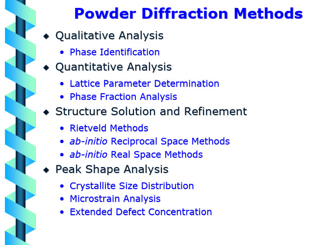
粉末衍射 powder_diffraction
N
Peak Intensities
• • •
N
Peak Shapes & Widths
• • •
Qualitative Analysis
N
The powder diffraction pattern of a known phase should act as a “fingerprint” which can be used to identify the phase. Computer “search-match” algorithms are used to compare experimental pattern with ICDD database of known compounds As of 1994 the International Centre for Diffraction Data (ICDD) database contained over 60,000 entries Can be used for multiphase mixtures Can be used to identify polymorphic mixtures
Rietveld Refinements
N
What is the goal of a Rietveld refinement? • To obtain an accurate crystal structure What is the basic idea of a Rietveld refinement? • To fit the entire diffraction pattern at once, optimizing the agreement between calculated and observed patterns
Using Sonnet in a Cadence Virtuoso Design Flow说明书

Using Sonnet in a Cadence Virtuoso Design FlowPurpose of this document:This document describes the Sonnet plug-in integration for the Cadence Virtuoso design flow,for silicon accurate EM modelling of passive structures.Using Sonnet in a Cadence Virtuoso Design Flow (1)Using Sonnet in a Cadence Virtuoso Design Flow (2)Sonnet Professional Key Benefits (3)Sonnet Professional Key Features (3)When to Use Sonnet EM Analysis (3)When to Use Sonnet EM Analysis (4)Sonnet EM Design Process (5)Example1 (12)Example2 (13)Example3 (14)Document revised:15.August2011Document revision:1.2Using Sonnet in a Cadence Virtuoso Design Flow The plug-in integration of the Sonnet Professional analysis program into the Cadence Virtuoso layout environment allows Cadence users to perform accurate EM modelling on selected Virtuoso cells,for physical verification of critical components and interconnections.This plug-in solution allows designers to extract a Sonnet EM analysis cell view directly from the layout view.Simulation results can be easily back annotated to the Cadence schematic.High precision electromagnetic(EM)analysis with Sonnet complements the traditional RC extraction tools.With Sonnet,simulation results include all physical effects like coupling, skin effect,proximity effect,surface waves and radiation.While traditional RC extraction tools like Cadence Assura are optimised to handle full chip extraction,Sonnet analysis is most suitable to rigorously analyze individual components,interconnects and smaller parts of a layout with very high confidence.With Sonnet,you can replace legacy3D finite element solvers,which are often not integrated into the Cadence design flow and require cumbersome and error prone manual modelling and data transfer.Sonnet Professional Key BenefitsSonnet Professional enables you to:∙Accurately model passive components (inductors,capacitors,resistors)to determine values like RLC and Q factor∙Accurately model multi layer interconnects and via structures∙Generate a technology accurate electrical model for arbitrary layout shapes ∙Quantify parasitic coupling between components,interconnects and vias ∙Include substrate induced effects like substrate loss∙Visualize the current flow in components,interconnects and viasSonnet Professional Key FeaturesThe key features of Sonnet Professional include:∙FFT based Method of Moments analysis for ultimate reliability and accuracy ∙Easy to learn,easy and efficient to use∙Only one high precision analysis engine –no need to switch between solvers ∙Conformal Meshing for very efficient high accuracy meshing of curved structures ∙Finite thickness modelling (including advanced n-sheet model)∙Dielectric bricks for truncated dielectric materials (e.g.MIM capacitor)∙Adaptive Band Synthesis for fast and reliable frequency sweeps with a minimum number of EM samples -more efficient than traditional approaches∙Easy to use data display for analysis results,including R,L,C,Q evaluation ∙Equation capability for pre-defined or customized calculation on simulated data ∙Seamless integration into the Cadence Virtuoso design environment∙All configuration and technology setup is menu /dialog based–no need to edit configuration text files∙Remote simulation capability∙Compatible with the LSF cluster and load balancing system ∙Sonnet Software Inc.is a Cadence Connectionspartner.Technology (Cadence library)Spectre SPICES/Y/Z-parametersBroad band SPICE model w/symbolsWhen to Use Sonnet EM AnalysisThe use of electromagnetic analysis with Sonnet Professional is especially valuable in the following design situations:When parasitic coupling is present.Parasitic coupling is not always easy to predict without using electromagnetic analysis.Even elements which are"sufficiently"far apart can suffer from parasitic coupling:inductive or capacitive coupling,resonance effects due to grounding and surface waves that might propagate at the substrate boundary under certain conditions.Sonnet Professional analysis is based on the physical properties of your technology and will account for such physical effects.When accurate circuit models are not available or circuit model parameters are out of range.Model based circuit simulators are based on models for a specific application, with limited parameter range.For example,only selected geometries,substrate types and substrate parameters are available.It is difficult to estimate the error induced by parameter extrapolation,so using models outside their designed parameter range is not suitable for critical applications.Whenever a layout feature cannot be described by a circuit model,due to its geometry or technology,the physics based analysis with Sonnet Professional will provide the answer. An example for this could be a special inductor,capacitor or transformer which is not included in the design kit.Sonnet can be used to analyze those components"on the fly",or generate a full library of components models with trust worth electrical results.Sonnet EM Design ProcessThe following steps describe a typical process for creating and simulating a design with Sonnet Professional for Cadence Virtuoso.Define the stack-up and material properties.A simulation model for Sonnet Professional contains a number of layered dielectrics,conductor levels at the interface between dielectric layers and vias to connect different conductor levels.To simulate a layout in Sonnet,these material properties and definitions("technology")are required.Typically,the EDA support group will define and qualify a technology file for a Cadence library and release that to the RFIC designers.This is an easy and straightforward process once the material properties are known,because that definition is fully menu and dialog driven.When a designer creates a Sonnet simulation view of a cell,that pre-defined Sonnet technology file will be automatically loaded from the Cadence library.Make Sonnet View.Based on the layout view of a cell,the designer can easily create the Sonnet analysis view for that cell.If the cell layout contains hierarchy,the hierarchy will be resolved to create a flattened Sonnet EM view.Define the analysis box.With Sonnet's FFT based approach to method of Moments,it is necessary to define a finite analysis area("box")and a uniform sampling resolution("cell size").This defines the granularity for the analysis,and usually requires a trade off between analysis time and accuracy.The user defined cell size is very useful to control the meshing density of very complex shapes,to avoid over-meshing the circuit without any need for manual clean-up.Assign port numbers and properties.In Sonnet,circuit ports connect the analysed structure withthe outer circuit.Different port types are available fordifferent purposes.Cadence pins can be converted to Sonnetports fully automatically,based on the defined mapping.Where needed,feed lines will be extended to the boundaryof the analysis area automatically,and de-embedded fromthe analysis results.Define analysis frequencies.Sonnet uses the Method of Moments where the circuit is analysed at different frequencies of interest.With the unique Adaptive Band Synthesis (ABS)in Sonnet,an accurate wide band response can be obtained from a minimum number of EM simulated data points within a given frequency range.Using ABS,the designer only needs to enter the start and stop frequency.Of course, composite frequency sweeps are also possible,as well as a"DC"point.Save state(optional).An optional step after setting up all these parameters is to store the current"state"of the analysis settings for later re-use.This way,all settings can be loaded into a similar project easily.Define desired output format(optional).The desired analysis results can be for example S/Y/Z parameters,a schematic symbol with ADS or Spectre frequency domain data or a schematic symbol for broad band SPICE extracted data.The designer can define the desired output data before starting the Sonnet EM simulation,or generate the data later as a post processing task after EM analysis has finished.View simulation model in Sonnet(optional).If desired,the designer can take the simulation model as a2D or3D view to Sonnet,and review it in the Sonnet model editor. This is especially useful for complex multi layer circuits.The Sonnet interface will keep track of any manual changes,to makes sure that the Virtuoso view and the Sonnet view stay in sync.Simulate the circuit.The simulation can be started from within Cadence Virtuoso.The Sonnet analysis monitor will show analysis progress and an estimate of the memory requirement and total simulation time.View simulation results.When the simulation is done,simulation results can be viewed with the Sonnet plotting tool.It is possible to plot already available results while the analysis engine is still analysing more frequencies.Parameters like inductor L and Q or capacitor C and Q can be plotted immediately by using pre-defined equations.When the current distribution is of interest,the simulation can be configured to store current density data.That data can be visualized in various ways as2D or3D graphs.For a better understanding of the circuit,the current density or charge visualization can also be animated over time or frequency.Current density results can be exported to a spread sheet for post processing.In the current density image shown here,note the smooth display of the current distribution,which shows high edge current(required to calculate the conductor losses properly)and current crowding.This is one indication of the high resolution and high precision of the Sonnet analysis result.Back annotate results to the Cadence schematic.When the Sonnet analysis is finished, results are available in different formats.This includes both S/Y/Z-parameters for frequency domain simulation,as well as a broad band SPICE extraction for time domain (SPICE)simulation.Cadence schematic symbols to hold those Sonnet results are created fully automatically, with all the required mapping files.A sub-circuit schematic for the analysed cell is also created fully automatically.Example1Octagon inductor in the IHP250nm technology(SGB25V)with thick metal effects modeled. The technology files for Sonnet EM analysis have been developed by Dr.Mühlhaus Consulting&Software GmbH and are available to IHP customers with the design kit. Design and Measurement courtesy of IHP MicroelectronicsMeasured vs.Calculatedpink=measuredblue=Sonnet resultExample2Octagon inductor in the IHP250nm technology(SGB25V)with thick metal effects modeled. The technology files for Sonnet EM analysis have been developed by Dr.Mühlhaus Consulting&Software GmbH and are available to IHP customers with the design kit. Design and Measurement courtesy of IHP MicroelectronicsMeasured vs.Calculatedpink=measuredblue=Sonnet resultExample39.25-turn Circular Spiral Inductor on100um Silicon(step-graded conductivity in substrate). 5insulating layers between1um and3um,thick metal effects modeledData and design courtesy of Motorola SPS/WISDMeasured vs.Calculatedred=measuredblue=Sonnet result。
NUMECA帮助文档(六)
第十二章跨叶片截面模块12.1绪言本章针对透平机械讲述快速三维跨叶片截面模块的分析过程。
这个模块是全自动完成的并且利用一些NUMECA工具。
此外,附加模块FINE™/Design2D这些工具联系起来,可以进行叶片重新设计,改善叶片表面压力分布,关于这些详见第13章。
这个模块假设流动是轴对称的,并且流面形状和厚度也由用户提供或由参数自动生成(利用根部和顶部边界)。
几何输入数据必须由用户提供:1、流面及叶片这个流面上的截面或2、完整的叶片轮廓及端壁本模块由网格自动生成与NS湍流方程组成。
在下一节讲述这个跨叶片截面模块的界面及对用户的建议。
12-4节讲述自动生成网格的理论和求解方程。
12-5节讲述几何数据和输出结果。
12-6讲述实例。
12-2跨叶片截面模块的界面在FINE™/Design2D界面之下运行跨叶片截面模块,这些可以高速,简单,交互式求解。
所有参数可以在用户界面中选取,并自动创建输入文件及求解。
监视工具,MonitorTurbo,可以在计算中和计算后检查收敛情况及结果。
它可以实时查看叶片表面压力分布的收敛过程及叶片几何形状。
结果分析利用NUMECA CFViwe™后处理工具进行,自动进入跨叶片截面模式。
几何数据以ASCII输入文件列出,但是求解参数定义及边界条件在这个界面中列出。
这个截面的描述由FINE™/Design2D界面中的菜单创建。
更详细的说明见12-5.12.2.1开始新的或打开现存S1面计算在开始界面下,Project Selection窗口允许创建新工程或打开现存工程。
对于创建新的跨叶片截面工程,按如下操作:1、单击按扭Create a New Project2、选取工程保存路径及输入文件名3、关闭Grid File Selection窗口,Design 2D不需要输入网格文件4、进入S1流面模块,菜单Modules/Design 2D如果要打开现存工程,在Project Selection窗口中单击Open an Existing Project 按扭,并在File chooser窗口中选取一个文件。
- 1、下载文档前请自行甄别文档内容的完整性,平台不提供额外的编辑、内容补充、找答案等附加服务。
- 2、"仅部分预览"的文档,不可在线预览部分如存在完整性等问题,可反馈申请退款(可完整预览的文档不适用该条件!)。
- 3、如文档侵犯您的权益,请联系客服反馈,我们会尽快为您处理(人工客服工作时间:9:00-18:30)。
∂F ∂g
with coefficients depending
on (c, g).
Again
repeated use of eqn() written as a quintic in z results in
∂F ∂g
being expressed
as
another quintic. Now the numerical technique to solve this quintic consists
Z = e−F =
Dφ1 Dφ2
exp
−
T
r[
1 2
(φ21
+
φ22)−cφ1φ2
+
(V
(φ1)+
V
(φ2))]
(6)
This model is also exactly solvable. But the free energy is not known as an explicit function of (c, g). However, a parametric form of the free energy is available in the form
(−12g)n(2n − 1)!
Zn = n!(n + 2)!
(3)
This clearly holds for all n.However, we are interested in the thermodynamic or the large-n limit. To this end we use
Γ(z) →z→∞
e−z√zz−1/2 [1 2π
+
1 12z
+
1 288z2
+
...]
(4)
for the Gamma-functionΓ(z).This gives
Zn
=n→∞
− (−1)n(√48)n 4π
n−7/2 [1
−
25 8n
...]
(5)
The exponential growth in n is non-universal and depends on V (φ). The
The Cosmological Constant Problem
The main difficulty with the abovementioned method is that ai(n) grow very rapidly with n reflecting the (non-universal)exponential growth of Zn.For example,Z10 ≃ 10100.In fact by the time one gets to around 100, various coefficients exceed the typical machine limits. Of course, special purpose
F
=
−
1 2
log
g z
−
1 g
z 0
dt t
g(t)
+
1 2g2
z dt g(t)2 + 1log(1 − c2) + 3
0t
2
4
(7)
2
where
g(z)
=
z (1 − 3z)2
−
c2z
+
ቤተ መጻሕፍቲ ባይዱ3c2z3
=
g
(8)
The numerical generation of Zn is done through the following sequence of
φ2
+
V
(φ)]
(1)
where φ is a N × N Hermitean matrix. When V (φ) = gφ4,the expression for F in the large-N limit is
F = − (−12g)n(2n − 1)!
(2)
n n!(n + 2)!
interpreting the coefficient of gn in this sum as the fixed area partition sum for an ensemble of random surfaces of fixed area n,one finds
finite
size
corrections
are
of
the
form
[1
−
25 n
+
..].
Next we consider the case of the Ising model coupled to random surfaces.
This is described by the two matrix model defined by
power law correction n−7/2 is universal and defines the string susceptiblity γ
to be γ = −b + 3 when the power law correction is n−b.In this example the
where ξi are coefficients depending on c.It should be noted that all a − i(n) vanish for negative n and in fact as z ≃ g for small g is the branch we are interested in, it follows that ai(n) = 0 for n < ia and that ai(i) = a1(1)i. It is also easy to see that a1(1) = (1 − c2)−1.
arXiv:hep-th/9807103v1 15 Jul 1998
On Finite Size Effects in d = 2 Quantum Gravity
N.D. Hari Dass Institute of Mathematical Sciences, Chennai 600 113, INDIA
Abstract
A systematic investigation is given of finite size effects in d = 2 quantum gravity or equivalently the theory of dynamically triangulated random surfaces.For Ising models coupled to random surfaces, finite size effects are studied on the one hand by numerical generation of the partition function to arbitrary accuracy by a deterministic calculus, and on the other hand by an analytic theory based on the singularity analysis of the explicit parametric form of the free energy of the corresponding matrix model. Both these reveal that the form of the finite size corrections, not surprisingly, depend on the string susceptibility.For the general case where the parametric form of the matrix model free energy is not explicitly known, it is shown how to perform the singularity analysis.All these considerations also apply to other observables like susceptibility etc.In the case of the Ising model it is shown that the standard Fisher-scaling laws are reproduced.
Let us begin with the case of so called ”pure gravity” which is mapped
1
to the one-matrix model described by the partition function
Z = e−F =
Dφ
exp
−
T
r[
1 2
n−1
a5(n) =
a1(m) · a4(n − m)
(11)
1
The computational requirements then grow as ≃ n6 if all ai(m); m ≤ n are to be evaluated.This is prohibitive. On the other hand the structure of
A study of finite size effects in statistical systems is of importance for a variety of reasons. It is indispensable for a more reliable interpretation of numerical data. As shown by Cardy in the context of systems with conformal invariance, finite size effects also codify the spectrum of the theory. In most cases finite size effects are estimated or parametrised by extrapolating the results of simulations carried out for various sizes. It is the purpose of this article to show how such finite size effects for two dimensdional quantum gravity systems can be studied systematically.