Decay Rate of Triaxially-Deformed Proton Emitters
Measurement of the form-factor ratios for D+ -- K l nu
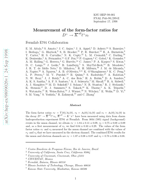
a r X i v :h e p -e x /9809026v 1 24 S e p 1998KSU-HEP-98-001FNAL Pub-98/289-E September 17,1998Measurement of the form-factor ratios forD +→K⋆0ℓ+νℓ,1Centro Brasileiro de Pesquisas F´ısicas,Rio de Janeiro,Brazil 2University of California,Santa Cruz,California 950643University of Cincinnati,Cincinnati,Ohio 452214CINVESTAV,Mexico5Fermilab,Batavia,Illinois 605106Illinois Institute of Technology,Chicago,Illinois 606167Kansas State University,Manhattan,Kansas 665068University of Massachusetts,Amherst,Massachusetts010039University of Mississippi,University,Mississippi3867710Princeton University,Princeton,New Jersey0854411Universidad Autonoma de Puebla,Mexico12University of South Carolina,Columbia,South Carolina2920813Stanford University,Stanford,California9430514Tel Aviv University,Tel Aviv,Israel15Box1290,Enderby,BC,V0E1V0,Canada16Tufts University,Medford,Massachusetts0215517University of Wisconsin,Madison,Wisconsin5370618Yale University,New Haven,Connecticut06511K⋆0ℓ+νℓare an especially clean way to study these effects because the leptonicand hadronic currents completely factorize in the decay amplitude.All informa-tion about the strong interactions can be parametrized by a few form factors.Also, according to Heavy Quark Effective Theory,the values of form factors for somesemileptonic charm decays can be related to those governing certain b-quark de-cays.In particular,the form factors studied here can be related to those for therare B–meson decays B→K⋆e+e−and B→K⋆γ[1,2]which provide windows for physics beyond the Standard Model.With a vector meson in thefinal state,there are four form factors,V(q2),A1(q2),A2(q2)and A3(q2),which are functions of the Lorentz-invariant momentum transfer squared[3].The differential decay rate for D+→K⋆0→K−π+is a quadratic homogeneous function of the four form factors.Unfortunately,the limited size of current data samples precludes precise measurement of the q2-dependence of the form factors;we thus assume the dependence to be given by the nearest-pole dominance model:F(q2)=F(0)/(1−q2/m2pole)where m pole= m V=2.1GeV/c2for the vector form factor V,and m pole=m A=2.5GeV/c2 for the three axial-vector form factors[4].The third form factor A3(q2),which is unobservable in the limit of vanishing lepton mass,probes the spin-0component of the off-shell W.Additional spin-flip amplitudes,suppressed by an overall factor of m2ℓ/q2when compared with spin no-flip amplitudes,contribute to the differential decay rate.Because A1(q2)appears among the coefficients of every term in the differential decay rate,it is customary to factor out A1(0)and to measure the ratios r V=V(0)/A1(0),r2=A2(0)/A1(0)and r3=A3(0)/A1(0).The values of these ratios can be extracted without any assumption about the total decay rate or the weak mixing matrix element V cs.We report new measurements of the form factor ratios for the muon chan-nel and combine them with slightly revised values of our previously publishedmeasurements of r V and r2[5]for the electron channel.This is thefirst set of measurements in both muon and electron channels from a single experiment.We also report thefirst measurement of r3=A3(0)/A1(0),which is unobservable in the limit of vanishing charged lepton mass.E791is afixed-target charm hadroproduction experiment[6].Charm particles were produced in the collisions of a500GeV/cπ−beam withfive thin targets, one platinum and four diamond.About2×1010events were recorded during the 1991-1992Fermilabfixed-target run.The tracking system consisted of23planes of silicon microstrip detectors,45planes of drift and proportional wire chambers, and two large-aperture dipole magnets.Hadron identification is based on the in-formation from two multicellˇCerenkov counters that provided good discrimination between kaons and pions in the momentum range6−36GeV/c.In this momentum range,the probabability of misidentifying a pion as a kaon depends on momentum but does not exceed5%.We identified muon candidates using a single plane of scintillator strips,oriented horizontally,located behind an equivalent of2.4meters of iron(comprising the calorimeters and one meter of bulk steel shielding).The an-gular acceptance of the scintillator plane was≈±62mrad×±48mrad(horizontally and vertically,respectively),which is somewhat smaller than that of the rest of the spectrometer for tracks which go through both magnets(≈±100mrad×±64mrad). The vertical position of a hit was determined from the strip’s vertical position,and the horizontal position of a hit from timing information.The event selection criteria used for this analysis are the same as for the electronic-mode form factor analysis[5],except for those related to lepton identifi-cation.Events are selected if they contain an acceptable decay vertex determined by the intersection point of three tracks that have been identified as a muon,a kaon,and a pion.The longitudinal separation between this candidate decay vertex and the reconstructed production vertex is required to be at least15times the esti-mated error on the separation.The two hadrons must have opposite charge.If the kaon and the muon have opposite charge,the event is assigned to the“right-sign”sample;if they have the same charge,the event is assigned to the“wrong-sign”sample used to model the background.To reduce the contamination from hadron decays inflight,only muon can-didates with momenta larger than8GeV/c are retained.With this momentum restriction,the efficiency of muon tagging was about85%,and the probability for a hadron to be identified as a muon was about3%.To exclude feedthrough from D+→K−π+π+,we exclude events in which the invariant mass of the three charged particles(with the muon candidate interpreted as a pion)is consistent with the D+mass.For ourfinal selection criteria,we use a binary-decision-tree algorithm(CART[7]),whichfinds linear combinations of parameters that have the highest discrimination power between signal and ing this algorithm,we found a linear combination of four discrimination variables[5]:(a)separation significance of the candidate decay vertex from target material;(b)distance of closest approach of the candidate D momentum vector to the primary vertex,taking into account the maximum kinematically-allowedmiss distance due to the unobserved neutrino;(c)product over candidate D decay tracks of the distance of closest approach of the track to the secondary vertex, divided by the distance of closest approach to the primary vertex,where each dis-tance is measured in units of measurement errors;and(d)significance of separation between the production and decay vertices.Thisfinal selection criterion reduced the number of wrong-sign events by50%,and the number of right-sign events by 25%.Although this does not affect our sensitivity substantially,it does reduce systematic uncertainties associated with the background subtraction.The minimum parent mass M min is defined as the invariant mass of Kπµνwhen the neutrino momentum component along the D+direction offlight is ignored.The distribution of M min should have a Jacobian peak at the D+mass,and we observe such a peak in our data(Fig.1).We retain events with M min in the range1.6 to2.0GeV/c2as indicated by the arrows in thefigure.The distribution of Kπinvariant mass for the retained events is shown in the top right of Fig.1for both right-sign and wrong-sign samples.Candidates with0.85<M Kπ<0.94GeV/c2 were retained,yieldingfinal data samples of3629right-sign and595wrong-sign events.The hadroproduction of charm,the differential decay rate,and the detector response were simulated with a Monte Carlo event generator.A sample of events was generated according to the differential decay rate(Eq.22in Ref.[3]),with the form factor ratios r V=2.00,r2=0.82,and r3=0.00.The same selection criteria were applied to the Monte Carlo events as to real data.Out of25million generated events,95579decays passed all cuts.Figure1(bottom)shows the distribution of M Kπfrom real data after background subtraction(“right-sign”minus“wrong-sign”)overlaid with the corresponding Monte Carlo distribution after all cuts are applied.The agreement between the two distributions suggests that wrong-sign events correctly account for the size of the background.The differential decay rate[3]is expressed in terms of four independent kine-matic variables:the square of the momentum transfer(q2),the polar angleθV in theK⋆0and W+decay planes.The definition we use for the polar angle θℓis related to the definition used in Ref.[3]byθℓ→π−θℓ.Semileptonic decays cannot be fully reconstructed due to the undetected neu-trino.With the available information about the D+direction offlight and the charged daughter particle momenta,the neutrino momentum(and all the decay’s kinematic variables)can be determined up to a two-fold ambiguity if the parent mass is constrained.Monte Carlo studies show that the differential decay rate is more accurately determined if it is calculated with the solution corresponding to the lower laboratory-frame neutrino momentum.To extract the form factor ratios the distribution of the data points in the four-dimensional kinematic variable space isfit to the full expression for the differential decay rate.We use the same unbinned maximum-likelihoodfitting technique as inour D+→K⋆0µ+νµcandidates as the previous method, but uses additional neutrino-momentum solutions.This is true for both the data and for the Monte Carlo sample used in the likelihood function calculation,so the results of thisfit could differ from those of the previousfit.The values of the form factor ratios obtained with the two methods agree well, providing further assurance that selecting the lower neutrino momentum solution in the primary method and correcting for the systematic bias gives the correct result.However,the systematic uncertainties for the primary method(see below) were found to be significantly smaller,mainly because the unbinned maximum-likelihood method is more stable against changes in the size of the phase spacevolume.Therefore,the primary method was chosen for quotingfinal results.We classify systematic uncertainties into three categories:(a)Monte Carlo simulation of detector effects and production mechanism;(b)fitting technique;(c) background subtraction.The estimated contributions of each are given in Table I. The main contributions to category(a)are due to muon identification and data selection criteria.The contributions to category(b)are related to the limited size of the Monte Carlo sample and to corrections for systematic bias.The measurements of the form factor ratios for D+→K⋆0e+νe[5]follow the same analysis procedure except for the charged lepton identification.Both results are listed in Table II.The consistency within errors of the results measured in the electron and muon channels supports the assumption that strong interaction effects,incor-porated in the values of form factor ratios,do not depend on the particular W+ leptonic decay.Based on this assumption,we combine the results measured for the electronic and muonic decay modes.The averaged values of the form factor ratios are r V=1.87±0.08±0.07and r2=0.73±0.06±0.08.The statistical and systematic uncertainties of the average results were determined using the general procedure described in Ref.[9](Eqns.3.40and3.40′).Some of the systematic errors for the two samples have positive correlation coefficients,and some nega-tive.The combination of all systematic errors is ultimately close to that which one would obtain assuming all the errors are uncorrelated.The third form factor ratio r3was not measured in the electronic mode.Table II compares the values of the form factor ratios r V and r2measured by E791in the electron,muon and combined modes with previous experimental results.The size of the data sample and the decay channel are listed for each case. All experimental results are consistent within errors.The comparison between the E791combined values of the form factor ratios r V and r2and previous experimental results is also shown in Fig.3(top).Table III and Fig.3(bottom)compare thefinal E791result with published theoretical predictions.The spread in the theoretical results is significantly larger than the E791experimental errors.To summarize,we have measured the values of the form factor ratios in the decay channel D+→K⋆0e+νe gives r V=1.87±0.08±0.07and r2=0.73±0.06±0.08.We gratefully acknowledge the assistance from Fermilab and other participat-ing institutions.This work was supported by the Brazilian Conselho Nacional de Desenvolvimento Cient´ıfico e Technol´o gico,CONACyT(Mexico),the Israeli Academy of Sciences and Humanities,the U.S.Departament of Energy,the U.S.-Israel Binational Science Foundation,and the U.S.National Science Foundation.REFERENCES[1]N.Isgur and M.B.Wise,Phys.Rev.D42(1990)2388.[2]Z.Ligeti,I.W.Stewart and M.B.Wise,Phys.Lett.B420(1998)359.[3]J.G.K¨o rner and G.A.Schuler,Phys.Lett.B226(1989)185.[4]Particle Data Group,Review of Particle Physics,Phys.Rev.D50(1994)1568.[5]Fermilab E791Collaboration,E.M.Aitala et al.,Phys.Rev.Lett.80(1998)1393.The E791electron result for r V quoted in this paper is0.06higher than the value reported in this reference because we have corrected for inaccuracies in the earlier modeling of the D+transverse momentum.[6]J.A.Appel,Ann.Rev.Nucl.Part.Sci.42(1992)367;D.J.Summers et al.,XXVII Rencontre de Moriond,Les Arcs,France(15-22March1992)417. [7]L.Brieman et al.,Classification and Regression Trees(Chapman and Hall,New York,1984).[8]D.M.Schmidt,R.J.Morrison,and M.S.Witherell,Nucl.Instrum.Methods A328(1993)547.[9]L.Lyons,Statistics for Nuclear and Particle Physicists(Cambridge UniversityPress,Cambridge,1986).[10]Fermilab E687Collaboration,P.L.Frabetti et al.,Phys.Lett.B307(1993)262.[11]Fermilab E653Collaboration,K.Kodama et al.,Phys.Lett.B274(1992)246.[12]Fermilab E691Collaboration,J.C.Anjos et al.,Phys.Rev.Lett.65(1990)2630.[13]D.Scora and N.Isgur,Phys.Rev.D52(1995)2783.We have used the q2-dependence assumed in thefits to our data to extrapolate the theoretical form factors from q2=q2max to q2=0.[14]M.Wirbel,B.Stech,and M.Bauer,Z.Phys.C29(1985)637.[15]T.Altomari and L.Wolfenstein,Phys.Rev.D37(1988)681.[16]F.J.Gilman and R.L.Singleton,Jr.,Phys.Rev.D41(1990)142.[17]B.Stech,Z.Phys.C75(1997)245.[18]C.W.Bernard,Z.X.El-Khadra,and A.Soni,Phys.Rev.D45(1992)869,Phys.Rev.D47(1993)998.[19]V.Lubicz,G.Martinelli,M.S.McCarthy,and C.T.Sachrajda,Phys.Lett.B274(1992)415.[20]A.Abada et al.,Nucl.Phys.B416(1994)675.[21]C.R.Alton et al.,Phys.Lett.B345(1995)513.[22]K.C.Bowler et al.,Phys.Rev.D51(1995)4905.[23]P.Ball,V.M.Braun,and H.G.Dosch,Phys.Rev.D44(1991)3567.[24]T.Bhattacharya and R.Gupta,Nucl.Phys.B(Proc.Suppl.)47(1996)481.TABLESTABLE I.The main contributions to uncertainties on the form factor ratios.Sourceσr2σrVσr3Hadron identification0.010.010.02 Muon identification0.040.060.10 Production mechanism0.010.010.02 Acceptance0.030.020.08 Cut selection0.030.040.09MC volume size0.020.020.12 Number of MC points0.010.010.18 Bias0.010.020.06No.of background events0.040.020.06 Background shape0.040.040.06 E7916000(e+µ)1.87±0.08±0.070.73±0.06±0.08 E7913000(µ)1.84±0.11±0.090.75±0.08±0.09 E7913000(e)1.90±0.11±0.090.71±0.08±0.09 E687[10]900(µ)1.74±0.27±0.280.78±0.18±0.10E653[11]300(µ)2.00+0.34−0.32±0.160.82+0.22−0.23±0.11E691[12]200(e)2.0±0.6±0.30.0±0.5±0.2TABLE parison of E791results with theoretical predictions for the form factor ratios r V and r2.Group r V r2ISGW2[13]2.01.3WSB[14]1.41.3KS[3]1.01.0AW/GS[15,16]2.00.8Stech[17]1.551.06BKS[18]1.99±0.22±0.330.70±0.16±0.17 LMMS[19]1.6±0.20.4±0.4ELC[20]1.3±0.20.6±0.3APE[21]1.6±0.30.7±0.4UKQCD[22]1.4+0.5−0.20.9±0.2BBD[23]2.2±0.21.2±0.2 LANL[24]1.78±0.070.68±0.11FIGURES01002003004005006001.251.51.7522.25M min (GeV/ c 2)E v e n t s / 40 M e V / c21002003004005006007000.70.80.91 1.1K π invariant mass (GeV/ c 2)E v e n t s / 10 M e V / c 2050100150200250300K π invariant mass (GeV/ c 2)E v e n t s / 5 M e V / c2FIG.1.Distributions of minimum parent mass M min and Kπinvariant mass for D +→050100150200cos θl (q 2/q 2max < 0.5)E v e n t s / 0.2050100150200cos θl (q 2/q 2max ≥ 0.5)E v e n t s / 0.250100150200cos θV (q 2/q 2max < 0.5)E v e n t s / 0.2050100150200cos θV (q 2/q 2max ≥ 0.5)E v e n t s / 0.250100150200χ (cos θV < 0)E v e n t s / 0.2π050100150200χ (cos θV ≥ 0)E v e n t s / 0.2πparison of single-variable distributions of background-subtracted data (crosses)with Monte Carlo predictions (dashed histograms)using best-fit values for the form factor ratios.1111.21.41.61.822.22.4rr V11.21.41.61.822.22.4r 2r VFIG.3.Top:Comparison of experimental measurements of form factor ratios r V and r 2for D +→。
委托代理模型的连续时间版本(Sannikov)
A Continuous-Time Version of the Principal-AgentProblem.Yuliy Sannikov∗March14,2007AbstractThis paper describes a new continuous-time principal-agent model,in which the output is a diffusion process with drift determined by the agent’s unobserved effort.The risk-averse agent receives consumption continuously.The optimal contract,basedon the agent’s continuation value as a state variable,is computed by a new methodusing a differential equation.During employment the output path stochasticallydrives the agent’s continuation value until it reaches a point that triggers retirement,quitting,replacement or promotion.The paper explores how the dynamics of theagent’s wages and effort,as well as the optimal mix of short-term and long-termincentives,depend on the contractual environment.1Keywords:Principal-agent model,continuous time,optimal contract,career path,retirement,promotionJEL Numbers:C63,D82,E2∗Correspondence should be sent to Yuliy Sannikov,University of California at Berkeley,Department of Economics,593Evans Hall,Berkeley,CA94720-3880;e-mail:sannikov@;cellphone (650)-303-7419.1I am most thankful to Michael Harrison for his guidance and encouragement to develop a rigorous continuous time model from my early idea and for helping me get valuable feedback,and to Andy Skrzypacz for a detailed review of the paper and for many helpful suggestions.I am also grateful to Darrell Duffie, Yossi Feinberg,Bengt Holmstrom,Chad Jones,Gustavo Manso,Paul Milgrom,John Roberts,Thomas Sargent,Sergio Turner and Robert Wilson for valuable feedback,and to Susan Athey for comments on an earlier version.1Introduction.The understanding of dynamic incentives is central in economics.How do companies moti-vate their workers through piecerates,bonuses,and promotions?How is income inequality connected with productivity,investment and economic growth?How dofinancial contracts and capital structure give incentives to the managers of a corporation?The methods and results of this paper provide important insights to many such questions.This paper introduces a continuous-time principal-agent model that focuses on the dynamic properties of optimal incentive provision.We identify factors that make the agent’s wages increase or decrease over time.We examine the degree to which current and future outcomes motivate the agent.We provide conditions under which the agent eventually reaches retirement in the optimal contract.We also investigate how the costs of creating incentives and the dynamic properties of the optimal contract depend on the contractual environment:the agent’s outside options,the difficulty of replacing the agent, and the opportunities for promotion.Our new dynamic insights are possible due to technical advantages of the continuous-time methods over the traditional discrete-time ones.Continuous time leads to a much simpler computational procedure tofind the optimal contract by solving an ordinary differ-ential equation.This equation highlights the factors that determine optimal consumption and effort.The dynamics of the agent’s career path is naturally described by the drift and volatility of the agent’s payoffs.The geometry of solutions to the differential equation allows for easy comparisons to see how the agent’s wages,effort and incentives depend on the contractual environment.Finally,continuous time highlights many essential features of the optimal contract,including the agent’s eventual retirement.In our benchmark model a risk-averse agent is tied to a risk-neutral principal forever after employment starts.The agent influences output by his continuous unobservable effort input.The principal sees only the output:a Brownian motion with a drift that depends on the agent’s effort.The agent dislikes effort and enjoys consumption.We assume that the agent’s utility function has the income effect,that is,as the agent’s income increases it becomes costlier to compensate him for effort.Also,we assume that the agent’s utility of consumption is bounded from below.At time0the principal can commit to any history-dependent contract.Such a contract specifies the agent’s consumption at every moment of time contingent on the entire past output path.The agent demands an initial reservation utility from the entire contract inorder to begin,and the principal offers a contract only if he can derive a positive profit from it.After we solve our benchmark model,we examine how the optimal contract changes if the agent may quit,be replaced or promoted.As in related discrete-time models,the optimal contract can be described in terms of the agent’s continuation value as a single state variable,which completely determines the agent’s effort and consumption.After any history of output the agent’s continuation value is the total future expected utility.The agent’s value depends on his future wages and effort.While in discrete time the optimal contract is described by cumbersome functions that map current continuation values and output realizations into future continuation values and consumption,continuous time offers more natural descriptors of employment dynamics: the drift and volatility of the agent’s continuation value.The volatility of the agent’s continuation value is related to effort.The agent has incentives to put higher effort when his value depends more strongly on output.Thus, higher effort requires a higher volatility of the agent’s value.The agent’s optimal effort varies with his continuation value.To determine optimal effort,the principal maximizes expected output minus the costs of compensating the agent for effort and the risk required by incentives.If the agent is very patient,so that incentive provision is costless,the optimal effort decreases with the agent’s continuation value due to the income effect.Apart from this extreme case,the agent’s effort is typically nonmonotonic because of the costs of exposing the agent to risk.The drift of the agent’s value is related to the allocation of payments over time.The agent’s value has an upward drift when his wages are backloaded,i.e.his current consump-tion is small relative to his expected future payoff.A downward drift of the agent’s value corresponds to frontloaded payments.The agent’s intertemporal consumption is distorted to facilitate the provision of incentives.The drift of the agent’s value always points in the direction where it is cheaper to provide the agent with incentives.Unsurprisingly,when the agent gets patient,so that incentive provision is costless,his continuation value does not have any drift.Over short time intervals,our optimal contract resembles that of Holmstrom and Mil-grom(1987)(hereafter HM),who study a simple continuous-time model in which the agent gets paid at the end of afinite time interval.HM show that optimal contracts are linear in aggregate output when the agent has exponential utility with a monetary cost of effort.2 2Many other continuous-time papers have extended the linearity results of HM.Schattler and Sung (1993)develop a more general mathematical framework for such results,and Sung(1995)allows the agentThese preferences have no income effect.According to Holmstrom and Milgrom(1991), the model of HM is“especially well suited for representing compensation paid over short period.”Therefore,it is not surprising that the optimal contract in our model is also approximately linear in incremental output over short time periods.In the long-run,the optimal contract involves complex nonlinear patterns of the agent’s wages and effort.In our benchmark setting,where the contract binds the agent to the principal forever,the agent eventually reaches retirement.After retirement,which occurs when the agent’s continuation value reaches a low endpoint or a high endpoint,the agent receives a constant stream of consumption and stops putting effort.Why must the agent retire when his continuation value reaches either endpoint?For the low retirement point,our assumption that the agent’s consumption utility is bounded from below implies that payments to the agent must stop when his value reaches the lower bound. On the other hand,when the agent’s continuation value becomes very high,although it is possible to keep the agent actively employed,retirement becomes optimal due to the income effect.When the agent’s consumption is high,it costs too much to compensate him for positive effort.Spear and Wang(2005)provide similar intuition in a two-period model.This intuition alone does not imply eventual retirement.There are many contracts,in which the agent suspends effort only temporarily and never retires.However,our results imply that those contracts are suboptimal.In the optimal contract,the agent’s continuation value has a strictly positive volatility,which eventually drives the agent to retirement with probability1.3Of course,retirement and other dynamic properties of the optimal contract depend on the contractual environment.The agent cannot be forced to stop consuming at the low retirement point if he has acceptable outside opportunities.Then,the agent quits instead of retiring at the low endpoint.If the agent is replaceable,the principal hires a new agent when the old agent reaches retirement.The high retirement point may also be replaced with promotion,an event that allows the agent to gain greater human capital,and manage larger and more important projects with higher expected output.4The contractual envirnoment matters for the dynamics of the agent’s wages.We already to control volatility as well.Hellwig and Schmidt(2002)look at the conditions for a discrete-time principal-agent model to converge to the HM solution.See also Bolton and Harris(2001),Ou-yang(2003)and Detemple,Govindaraj and Loewenstein(2001)for further generalization and analysis of the HM setting.3Eventual retirement in the optimal contract depends on the assumption that the agent is equally patient as the principal.See DeMarzo and Sannikov(2006),Farhi and Werning(2006a)and Sleet and Yeltekin(2006)for examples where the agent is less patient than the principal.4I thank the editor Juuso Valimaki for encouraging me to investigate this possibility.mentioned that the drift of the agent’s continuation value always points in the direction where it is cheaper to create incentives.Since better outside options make it more difficult to motivate and retain the agent,it is not surprising that wages become more backloaded with better outside options.Lower payments up front cause the agent’s continuation value to drift up,away from the point where he is forced to quit.When the employer can offer better promotion opportunities,the agent’s wages also become backloaded in the optimal contract.The agent is willing to work for lower wages up front when he is motivated by future promotions.Thesefindings highlight the factors that may affect the agent’s wage structure in internal labor markets.What matters more for the agent’s incentives:immediate outcomes or those in distant future?Contracts in practice use both short-term incentives,as piecework and bonuses, and long-term ones,as promotions and permanent wage increases.In our model,the ratio of the volatilities of the agent’s consumption and his continuation value measures the mix of short-term and long-term incentives.Wefind that the optimal contract uses stronger short-term incentives when the agent has better outside options,which interfere with the agent’s incentives in the long run.In contrast,when the principal has greaterflexibility to replace or promote the agent,the optimal contract uses stronger long-term incentives and keeps the agent’s wages more constant in the short run.Wefind that the agent puts higher effort and the principal gets greater profit when the optimal contract relies on stronger long-term incentives.It is difficult to study these dynamic properties of the optimal contract using discrete-time models.Without theflexibility of the differential equation that describes the dynamics of the optimal contract in continous time,traditional discrete-time models produce a more limited set of results.Spear and Srivastava(1987)show that how to analyze dynamic principal-agent problems in discrete time using recursive methods,with the agent’s contin-uation value as a state variable.5Assuming that the agent’s consumption is nonnegative and that his utility is separable in consumption and effort,that paper shows that inverse of the agent’s marginal utility of consumption is a martingale.An earlier paper of Rogerson (1985)demonstrates this result on a two-period model.6However,this restriction is not very informative about the optimal path of the agent’s wages,since a great diversity of 5Abreu,Pearce and Stacchetti(1986)and(1990)study the recursive structure of general repeated games.6This condition,called the inverse Euler equation,has received a lot of attention in recent macroeco-nomics literature.For example,see Golosov,Kocherlakota and Tsyvinski(2003)and Farhi and Werning (2006b).consumption profiles in different contractual environments we study satisfy this restriction.In its early stage,this paper was inspired by Phelan and Townsend(1991)who develop a method for computing optimal long-term contracts in discrete time.There are strong similarities between our continuous-time solutions and their discrete-time example,imply-ing that ultimately the two approaches are different ways of looking at the same thing. Their computational method relies on linear programming and multiple iterations to con-verge to the principal’s value function.While their method is quiteflexible and applicable to a wide range of settings,it is far more computationally intensive than our method of solving a differential equation.Because general discrete-time models are difficult to deal with,one may be tempted to restrict attention to the special tractable case when the agent is patient.As the agent’s discount rate converges to0,efficiency becomes attainable,as shown in Radner(1985)and Fudenberg,Holmstrom and Milgrom(1990).7However,wefind that optimal contracts when the agent is patient do not deliver many important dynamic insights:the agent’s continuation value becomes driftless,and the agent’s effort,determined without taking the cost of incentives into account,is decreasing in the agent’s value.Concurrently with this paper,Williams(2003)also develops a continuous-time principal-agent model.The aim of that paper is to present a general characterization of the optimal contract using a partial differential equation and forward and backward stochastic differ-ential equations.The resulting contract is written recursively using several state variables, but due to greater generality,the optimal contract is not explored in as much detail.More recently,a number of other papers started using continuous-time methodology. DeMarzo and Sannikov(2006)study the optimal contract in a cash-flow deversion model using the methods from this paper.Biais et al.(2006)show that the contract of DeMarzo and Sannikov(2006)arises in the limit of discrete-time models as the agent’s actions become more frequent.Cvitanic,Wan and Zhang(2006)study optimal contracts when the agent gets paid once,and Westerfield(2006)develops an approach that uses the agent’s wealth, as opposed to his continuation value,as a state variable.The paper is organized as follows.Section2presents the benchmark setting and for-mulates the principal’s problem.Section3presents an optimal contract and discusses its properties:the agent’s effort and consumption,the drift and volatility of his continuation value and retirement points.The formal derivation of the optimal contract is deferred to the Appendix.Section4explores how the agent’s outside options and the possibilities for 7Also,Fudenberg,Levine and Maskin(1994)prove a Folk Theorem for general repeated games.replacement and promotion affect the dynamics of the agent’s wages,effort and incentives. Section5studies optimal contracts for small discount rates.Section6concludes the paper.2The Benchmark Setting.Consider the following dynamic principal-agent model in continuous time.A standard Brownian motion Z={Z t,F t;0≤t<∞}on(Ω,F,Q)drives the output process.The total output X t produced up to time t evolves according todX t=A t dt+σdZ t,where A t is the agent’s choice of effort level andσis a constant.The agent’s effort is a stochastic process A={A t∈A,0≤t<∞}progressively measurable with respect to F t, where the set of feasible effort levels A is compact with the smallest element0.The agent experiences cost of effort v(A t),measured in the same units as the utility of consumption, where v:A→ is continuous,increasing and convex.We normalize v(0)=0and assume that there isγ0>0such that v(a)≥γ0a for all a∈A.The output process X is publicly observable by both the principal and the agent.The principal does not observe the agent’s effort A,and uses the observations of X to give the agent incentives to make costly effort.Before the agent starts working for the principal,the principal offers him a contract that specifies a nonnegativeflow of consumption C t(X s;0≤s≤t)∈[0,∞)based on the principal’s observation of output.The principal can commit to any such contract.We assume that the agent’s utility is bounded from below and normalize u(0)=0.Also,we assume that u:[0,∞)→[0,∞)is an increasing,concave and C2function that satisfies u (c)→0as c→∞.For simplicity,assume that both the principal and the agent discount theflow of profit and utility at a common rate r.If the agent chooses effort level A t,0≤t<∞,his average expected utility is given byE r ∞0e−rt(u(C t)−v(A t))dt ,and the principal gets average profitE r ∞0e−rt dX t−r ∞0e−rt C t dt =E r ∞0e−rt(A t−C t)dt .Factor r in front of the integrals normalizes total payoffs to the same scale asflow payoffs.We say that an effort process{A t,0≤t<∞}is incentive compatible with respect to {C t,0≤t<∞}if it maximizes the agent’s total expected utility.2.1The Formulation of The Principal’s Problem.The principal’s problem is to offer a contract to the agent:a stream of consumption {C t,0≤t<∞}contingent on the realized output and an incentive-compatible advice of effort{A t,0≤t<∞}that maximizes the principal’s profitE r ∞0e−rt(A t−C t)dt (1) subject to delivering to the agent a required initial value of at leastˆWE r ∞0e−rt(u(C t)−v(A t))dt ≥ˆW.(2) We assume that the principal can choose not to employ the agent,so we are only interested in contracts that generate nonnegative profit for the principal.3The Optimal Contract.This section describes the optimal contract for the benchmark model and discusses its basic properties.Appendix A provides the formal derivation of the optimal contract.It turns out that under the optimal contract the principal retires the agent after some paths of output by giving the agent a constant stream of payments in return for zero effort. The principal’s retirement profit as a function of the agent’s value F0:[0,u(∞))→(−∞,0] is given byF0(u(c))=−c,where u(∞)=lim c→∞u(c)can be infinity or afinite number.Even though retiring the agent may appear wasteful,wefind that under the optimal contract the agent ends up in retirement infinite time with probability1.88While in our model the agent keeps producing output with zero drift after retirement,it may be more natural to think that instead the principal shuts down thefirm.Analytically,the two possibilities are equivalent.Defineγ(a)=min{y∈[0,∞):a∈arg maxa∈Aya−v(a)}(3) The optimal contract is characterized by the unique concave solution F≥F0of the HJB equationF (W)=mina>0,c F(W)−a+c−F (W)(W−u(c)+v(a))rσ2γ(a)2/2(4)that satisfies the boundary conditionsF(0)=0,F(W gp)=F0(W gp)and F (W gp)=F 0(W gp)(5) for some W gp≥0,where F (W gp)=F 0(W gp)is called the smooth-pasting condition.9Let functions c:(0,W gp)→0and a:(0,W gp)→0be the minimizers in equation(4)on (0,W gp).A typical form of the value function F(0)together with a(W),c(W)and the drift of the agent’s continuation value(see below)are shown in Figure1.Theorem1,which is proved in Appendix A,characterizes optimal contracts.Theorem1.The unique concave function F≥F0that satisfies(4)and(5)character-izes any optimal contract with positive profit to the principal.For the agent’s starting value of W0>W gp,F(W0)<0is an upper bound on the principal’s profit.If W0∈[0,W gp], then the optimal contract attains profit F(W0).Such contract is based on the agent’s continuation value as a state variable,which starts at W0and evolves according todW t=r(W t−u(C t)+v(A t))dt+rγ(A t)(dX t−A t dt)(6) under payments C t=c(W t)and effort A t=a(W t),until the retirement timeτ.Retirement occurs when W t hits0or W gp for thefirst time.After retirement the agent gets constant consumption of−F0(Wτ)and puts effort0.The agent’s continuation value is his future expected payoffafter a given history of output.The intuition why the agent’s continuation value W t completely summarizes the past history in the optimal contract is the same as in discrete time.The agent’s incentives are unchanged if we replace the continuation contract that follows a given history with a9If r is sufficiently large,then the solution of(4)with boundary conditions F(0)=0and F (0)=F(0) satisfies F(W)>F0(W)for all W>0.In this case W gp=0and contracts with positive profit do not exist.-0.2-0.4-0.6-0.8√c,v(a)=0.5a2+0.4a,r=0.1andσ=1.Point W∗is Figure1:Function F for u(c)=the maximum of F.different contract that has the same continuation value W t.10Therefore,to maximize the principal’s profit after any history,the continuation contract must be optimal given W t. It follows that the agent’s continuation value W t completely determines the continuation contract.Equation(6)that describes the evolution of W t satisfies three objectives:incentives, promise keeping and profit maximization.The agent’s incentives arise from the sensitivity rγ(a)of his promised value towards output.Intuitively,it is optimal for the agent to choose the effort level a that maximizes the expected change of his promised value due to effort 10This logic would fail if the agent had hidden savings.With hidden savings,the agent’s past incentives to save depend not only on his current promised value,but also on how his value would change with savings level.Therefore,the problem with hidden savings has a different recursive structure,as discussed in the conclusions.minus the cost of effortr(γ(a)a−v(a)),where a is the drift of output when the agent chooses effort a.Functionγ(a)defined by (3)motivates the agent to put effort a with minimal volatility of continuation values.Due to the concavity of the principal’s profit,it is optimal to expose agent to the least amount of risk for a given effort level.Functionγ(a)is increasing in a.For the binary action case A={0,a},γ(a)=v(a)/a.When A is an interval and v is a differentiable function,γ(a)=v (a)for a>0.When the agent takes the recommended effort A t,then the drift r(W t−u(C t)+v(A t)) of the agent’s continuation value accounts for promise keeping.In order for W t to correctly describe the principal’s debt to the agent,in expectation W t grows at the interest rate r and fall due to theflow of repayments r(u(C t)−v(A t)).The HJB equation,which is the continuous-time version of the Bellman equation,deliv-ers the optimal choice of payments C t=c(W t)and recommendations of effort A t=a(W t). Equation(4),which is suitable for computation because it isolates F (W)on the left hand side,follows from the standard formrF(W)=maxa,c r(a−c)+r(W−u(c)+v(a))F (W)+r2σ2γ(a)2F (W)2(7)This equation determines a(W)and c(W)by maximizing the sum of the principal’s current expected profitflow r(a−c)and the expected change of his future profit due to the drift and volatility of the agent’s continuation value.Together,they add up to the annuity value of total profit rF(W).The optimal effort maximizesra+rv(a)F (W)+r2σ2γ(a)2F (W)2,(8)where ra is the expectedflow of output,−rv(a)F (W)is the cost of compensating the agent for his effort,and−r2σ2γ(a)2F (W)is the cost of exposing the agent to income uncertainty to provide incentives.These two costs typically work in opposite directions,creating a complex effort profile(see Figure1).While F (W)decreases in W because F is concave, F (W)tends increases over some ranges of W.11However,as r→0,the cost of exposing11F (W)increases at least on the interval[0,W∗],where c=0and sign F (W)=sign(rW−u(c)+ v(a))>0(see Theorem2).When W is smaller,the principal faces a greater risk of triggering retirementthe agent to risk goes away and the effort profile becomes decreasing in W,except possibly near endpoints0and W gp(see Section5).The optimal choice of consumption maximizes−c−F (W)u(c).(9)Thus,the agent’s consumption is0when F (W)≥−1/u (0),in the probationary interval [0,W∗∗],and it is increasing in W according to F (W)=−1/u (c)above W∗∗.Intuitively, 1/u (c)and−F (W)are the marginal costs of giving the agent value through current con-sumption and through his continuation payoff,respectively.Those marginal costs must be equal under the optimal contract,except in the probationary interval.There,consumption zero is optimal because it maximizes the drift of W t away from the inefficient low retirement point.The drift of W t is connected with the allocation of the agent’s wages over time.Section 5shows that the drift of W t becomes zero when the agent become patient,to minimize intertemporal distortions of the agent’s consumption.In general,the drift of W t is nonzero in the optimal contract.Theorem2shows that the drift of W t always points in the direction where it is cheaper to provide incentives.Theorem2.Until retirement,the drift of the agent’s continuation value points in the direction in which F (W)is increasing.Proof.From(7)and the Envelope Theorem,we haver(W−u(c)+v(a))F (W)+r2σ2γ(a)2F (W)2=0(10)Since F (W)is always negative,W−u(c)+v(a)has the same sign as F (W).QEDBy Ito’s lemma,(10)is the drift of−1/u (C t)=F (W t)on[W∗∗,W gp].Thus,in our model the inverse of the agent’s marginal utility is a martingale when the agent’s consump-tion is positive.The analogous result in discrete time wasfirst discovered by Rogerson (1985).Under the optimal contract the agent keeps putting effort at all times until he is even-tually retired when W t reaches0or W gp.The principal must retire the agent when W t hits 0because the only way to deliver to the agent value0is to pay him0forever.Indeed,if the future payments were not always0,the agent can guarantee himself a strictly positive value by providing stronger incentives.by putting effort0.Why is it optimal for the principal to retire agent if his continuation payoffbecomes sufficiently large?This happens due to the income effect:when theflow of payments to the agent is large enough,it costs the principal too much to compensate the agent for his effort,so it is optimal to allow effort0.When the agent gets richer, the monetary cost of delivering utility to the agent rises indefinitely(since u (c)→0as c→∞)while the utility cost of output stays bounded above0since v(a)≥γ0a for all a. High retirement occurs even before the cost of compensating the agent for effort exceeds the expected output from effort,since the principal must compensate the agent not only for effort,but also for risk(see(8)).While it is necessary to retire the agent when W t hits 0and it is optimal to do so if W t reaches W gp,there are contracts that prevent W t from reaching0or W gp by allowing the agent to suspend effort temporarily.Those contracts are suboptimal:in the optimal contract the agent puts positive effort until he is retired forever.12In the next subsection we discuss the paths of the agent’s continuation value and income, and the connections between the agent’s incentives,productivity and income distribution in the example in Figure1.Before that,we make three remarks about possible extensions of our model.Remark1:Retirement.If the agent’s utility was unbounded from below(e.g.expo-nential utility),our differential equation would still characterize the optimal contract,but the agent may never reach retirement at the low endpoint.To take care of this possibility, the boundary condition F(0)=0would need to be replaced with a regularity condition on the asymptotic behavior of F.Of course,the low retirement point does not disappear if the agent has an outside option at all times(see Section4).Similarly,if the agent’s utility had no income effect,the high retirement point may disappear as well.This would be the case if we assumed exponential utility with a monetary cost of effort,as in Holmstrom and Milgrom(1987).13Remark2:Savings.We assume in this model that the agent cannot save or borrow, and is restricted to consume what the principal pays him at every moment of time.What 12This conclusion depends on the assumption that the agent’s discount rate is the same as that of the principal.If the agent’s discount rate was higher,the optimal contract may allow the agent to suspend effort temporarily.13DeMarzo and Sannikov(2006)study a dynamic agency problem without the income effect.In their setting the moral hazard problem is that the agent may secretly divert cash from thefirm,so his benefit from the hidden action is measured in monetary terms.The optimal contract has a low absorbing state, since the agent’s utility is bounded from below,but no upper absorbing state.。
decay of correlation 数学名词

decay of correlation 数学名词Decay of correlation(相关性的衰减)refers to the decrease in correlation between two variables as the distance between them increases. It is a mathematical concept used to quantify the relationship between two variables across different spatial or temporal distances.1. The decay of correlation between rainfall and crop yield was observed as the distance between the two fields increased.雨量与农作物产量之间的相关性随着两个田地之间的距离增加而减弱。
2. The study analyzed the decay of correlation between interest rates and stock market performance over a one-year timespan.该研究分析了利率和股市表现之间的相关性在一年的时间内是如何衰减的。
3. As the distance between two cities increased, thedecay of correlation between their population sizes became more noticeable.随着两个城市之间的距离增加,它们的人口规模之间的相关性衰减变得更加明显。
4. The researchers used statistical methods to determine the decay of correlation between air pollution andrespiratory diseases in different neighborhoods.研究人员使用统计方法来确定不同社区之间空气污染和呼吸道疾病之间的相关性衰减。
yantubbs-The hardening soil model, Formulation and verification

The hardening soil model: Formulation and verificationT. SchanzLaboratory of Soil Mechanics, Bauhaus-University Weimar, GermanyP.A. VermeerInstitute of Geotechnical Engineering, University Stuttgart, GermanyP.G. BonnierP LAXIS B.V., NetherlandsKeywords: constitutive modeling, HS-model, calibration, verificationABSTRACT: A new constitutive model is introduced which is formulated in the framework of classical theory of plasticity. In the model the total strains are calculated using a stress-dependent stiffness, different for both virgin loading and un-/reloading. The plastic strains are calculated by introducing a multi-surface yield criterion. Hardening is assumed to be isotropic depending on both the plastic shear and volumetric strain. For the frictional hardening a non-associated and for the cap hardening an associated flow rule is assumed.First the model is written in its rate form. Therefor the essential equations for the stiffness mod-ules, the yield-, failure- and plastic potential surfaces are given.In the next part some remarks are given on the models incremental implementation in the P LAXIS computer code. The parameters used in the model are summarized, their physical interpre-tation and determination are explained in detail.The model is calibrated for a loose sand for which a lot of experimental data is available. With the so calibrated model undrained shear tests and pressuremeter tests are back-calculated.The paper ends with some remarks on the limitations of the model and an outlook on further de-velopments.1INTRODUCTIONDue to the considerable expense of soil testing, good quality input data for stress-strain relation-ships tend to be very limited. In many cases of daily geotechnical engineering one has good data on strength parameters but little or no data on stiffness parameters. In such a situation, it is no help to employ complex stress-strain models for calculating geotechnical boundary value problems. In-stead of using Hooke's single-stiffness model with linear elasticity in combination with an ideal plasticity according to Mohr-Coulomb a new constitutive formulation using a double-stiffness model for elasticity in combination with isotropic strain hardening is presented.Summarizing the existing double-stiffness models the most dominant type of model is the Cam-Clay model (Hashiguchi 1985, Hashiguchi 1993). To describe the non-linear stress-strain behav-iour of soils, beside the Cam-Clay model the pseudo-elastic (hypo-elastic) type of model has been developed. There an Hookean relationship is assumed between increments of stress and strain and non-linearity is achieved by means of varying Young's modulus. By far the best known model of this category ist the Duncan-Chang model, also known as the hyperbolic model (Duncan & Chang 1970). This model captures soil behaviour in a very tractable manner on the basis of only two stiff-ness parameters and is very much appreciated among consulting geotechnical engineers. The major inconsistency of this type of model which is the reason why it is not accepted by scientists is that, in contrast to the elasto-plastic type of model, a purely hypo-elastic model cannot consistently dis-tinguish between loading and unloading. In addition, the model is not suitable for collapse load computations in the fully plastic range.12These restrictions will be overcome by formulating a model in an elasto-plastic framework in this paper. Doing so the Hardening-Soil model, however, supersedes the Duncan-Chang model by far. Firstly by using the theory of plasticity rather than the theory of elasticity. Secondly by includ-ing soil dilatancy and thirdly by introducing a yield cap.In contrast to an elastic perfectly-plastic model, the yield surface of the Hardening Soil model is not fixed in principal stress space, but it can expand due to plastic straining. Distinction is made between two main types of hardening, namely shear hardening and compression hardening. Shear hardening is used to model irreversible strains due to primary deviatoric loading. Compression hardening is used to model irreversible plastic strains due to primary compression in oedometer loading and isotropic loading.For the sake of convenience, restriction is made in the following sections to triaxial loading conditions with 2σ′ = 3σ′ and 1σ′ being the effective major compressive stress.2 CONSTITUTIVE EQUATIONS FOR STANDARD DRAINED TRIAXIAL TESTA basic idea for the formulation of the Hardening-Soil model is the hyperbolic relationship be-tween the vertical strain ε1, and the deviatoric stress, q , in primary triaxial loading. When subjected to primary deviatoric loading, soil shows a decreasing stiffness and simultaneously irreversible plastic strains develop. In the special case of a drained triaxial test, the observed relationship be-tween the axial strain and the deviatoric stress can be well approximated by a hyperbola (Kondner& Zelasko 1963). Standard drained triaxial tests tend to yield curves that can be described by:The ultimate deviatoric stress, q f , and the quantity q a in Eq. 1 are defined as:The above relationship for q f is derived from the Mohr-Coulomb failure criterion, which involves the strength parameters c and ϕp . As soon as q = q f , the failure criterion is satisfied and perfectly plastic yielding occurs. The ratio between q f and q a is given by the failure ratio R f , which should obviously be smaller than 1. R f = 0.9 often is a suitable default setting. This hyperbolic relationship is plotted in Fig. 1.2.1 Stiffness for primary loadingThe stress strain behaviour for primary loading is highly nonlinear. The parameter E 50 is the con-fining stress dependent stiffness modulus for primary loading. E 50is used instead of the initial modulus E i for small strain which, as a tangent modulus, is more difficult to determine experimen-tally. It is given by the equation:ref E 50is a reference stiffness modulus corresponding to the reference stress ref p . The actual stiff-ness depends on the minor principal stress, 3σ′, which is the effective confining pressure in a tri-axial test. The amount of stress dependency is given by the power m . In order to simulate a loga-rithmic stress dependency, as observed for soft clays, the power should be taken equal to 1.0. As a3Figure 1. Hyperbolic stress-strain relation in primary loading for a standard drained triaxial test.secant modulus ref E 50 is determined from a triaxial stress-strain-curve for a mobilization of 50% ofthe maximum shear strength q f .2.2 Stiffness for un-/reloadingFor unloading and reloading stress paths, another stress-dependent stiffness modulus is used:where ref urE is the reference Young's modulus for unloading and reloading, corresponding to the reference pressure σ ref . Doing so the un-/reloading path is modeled as purely (non-linear) elastic.The elastic components of strain εe are calculated according to a Hookean type of elastic relation using Eqs. 4 + 5 and a constant value for the un-/reloading Poisson's ratio υur .For drained triaxial test stress paths with σ2 = σ3 = constant, the elastic Young's modulus E ur re-mains constant and the elastic strains are given by the equations:Here it should be realised that restriction is made to strains that develop during deviatoric loading,whilst the strains that develop during the very first stage of the test are not considered. For the first stage of isotropic compression (with consolidation), the Hardening-Soil model predicts fully elastic volume changes according to Hooke's law, but these strains are not included in Eq. 6.2.3 Yield surface, failure condition, hardening lawFor the triaxial case the two yield functions f 12 and f 13 are defined according to Eqs. 7 and 8. Here4Figure 2. Successive yield loci for various values of the hardening parameter γ p and failure surface.the measure of the plastic shear strain γ p according to Eq. 9 is used as the relevant parameter forthe frictional hardening:with the definitionIn reality, plastic volumetric strains p υε will never be precisely equal to zero, but for hard soils plastic volume changes tend to be small when compared with the axial strain, so that the approxi-mation in Eq. 9 will generally be accurate.For a given constant value of the hardening parameter, γ p , the yield condition f 12 = f 13 = 0 can be visualised in p'-q-plane by means of a yield locus. When plotting such yield loci, one has to use Eqs. 7 and 8 as well as Eqs. 3 and 4 for E 50 and E ur respectively. Because of the latter expressions,the shape of the yield loci depends on the exponent m . For m = 1.0 straight lines are obtained, but slightly curved yield loci correspond to lower values of the exponent. Fig. 2 shows the shape of successive yield loci for m = 0.5, being typical for hard soils. For increasing loading the failure sur-faces approach the linear failure condition according to Eq. 2.2.4 Flow rule, plastic potential functionsHaving presented a relationship for the plastic shear strain, γ p , attention is now focused on the plastic volumetric strain p υε. As for all plasticity models, the Hardening-Soil model involves a re-lationship between rates of plastic strain, i.e. a relationship between p υε and p γ . This flow rule hasthe linear form:5Clearly, further detail is needed by specifying the mobilized dilatancy angle m ψ. For the presentmodel, the expression:is adopted, where cv ϕ is the critical state friction angle, being a material constant independent ofdensity (Schanz & Vermeer 1996), and m ϕ is the mobilized friction angle:The above equations correspond to the well-known stress-dilatancy theory (Rowe 1962, Rowe 1971), as explained by (Schanz & Vermeer 1996). The essential property of the stress-dilatancy theory is that the material contracts for small stress ratios m ϕ < cv ϕ, whilst dilatancy occurs for high stress ratios m ϕ < cv ϕ. At failure, when the mobilized friction angle equals the failure angle,p ϕ, it is found from Eq. 11 that:Hence, the critical state angle can be computed from the failure angles p ϕand p ψ. The above defi-nition of the flow rule is equivalent to the definition of definition of the plastic potential functionsg 12 and g 13 according to:Using theKoiter-rule (Koiter 1960) for yielding depending on two yield surfaces (Multi-surface plasticity ) one finds:Calculating the different plastic strain rates by this equation, Eq. 10 directly follows.3 TIME INTEGRATIONThe model as described above has been implemented in the finite element code P LAXIS (Vermeer& Brinkgreve 1998). To do so, the model equations have to be written in incremental form. Due to this incremental formulation several assumptions and modifications have to be made, which will be explained in this section.During the global iteration process, the displacement increment follows from subsequent solu-tion of the global system of equations:where K is the global stiffness matrix in which we use the elastic Hooke's matrix D , f ext is a global load vector following from the external loads and f int is the global reaction vector following from the stresses. The stress at the end of an increment σ 1 can be calculated (for a given strain increment ∆ε) as:6whereσ0 , stress at the start of the increment,∆σ , resulting stress increment,4D , Hooke's elasticity matrix, based on the unloading-reloading stiffness,∆ε , strain increment (= B ∆u ),γ p , measure of the plastic shear strain, used as hardening parameter,∆Λ , increment of the non-negative multiplier,g , plastic potential function.The multiplier Λ has to be determined from the condition that the function f (σ1, γ p ) = 0 has to be zero for the new stress and deformation state.As during the increment of strain the stresses change, the stress dependant variables, like the elasticity matrix and the plastic potential function g , also change. The change in the stiffness during the increment is not very important as in many cases the deformations are dominated by plasticity.This is also the reason why a Hooke's matrix is used. We use the stiffness matrix 4D based on the stresses at the beginning of the step (Euler explicit ). In cases where the stress increment follows from elasticity alone, such as in unloading or reloading, we iterate on the average stiffness during the increment.The plastic potential function g also depends on the stresses and the mobilized dilation angle m ψ. The dilation angle for these derivatives is taken at the beginning of the step. The implementa-tion uses an implicit scheme for the derivatives of the plastic potential function g . The derivatives are taken at a predictor stress σtr , following from elasticity and the plastic deformation in the previ-ous iteration:The calculation of the stress increment can be performed in principal stress space. Therefore ini-tially the principal stresses and principal directions have to be calculated from the Cartesian stresses, based on the elastic prediction. To indicate this we use the subscripts 1, 2 and 3 and have 321σσσ≥≥ where compression is assumed to be positive.Principal plastic strain increments are now calculated and finally the Cartesian stresses have to be back-calculated from the resulting principal constitutive stresses. The calculation of the consti-tutive stresses can be written as:From this the deviatoric stress q (σ1 – σ3) and the asymptotic deviatoric stress q a can be expressed in the elastic prediction stresses and the multiplier ∆Λ:7whereFor these stresses the functionshould be zero. As the increment of the plastic shear strain ∆γ p also depends linearly on the multi-plier ∆Λ, the above formulae result in a (complicated) quadratic equation for the multiplier ∆Λwhich can be solved easily. Using the resulting value of ∆Λ, one can calculate (incremental)stresses and the (increment of the) plastic shear strain.In the above formulation it is assumed that there is a single yield function. In case of triaxial compression or triaxial extension states of stress there are two yield functions and two plastic po-tential functions. Following (Koiter 1960) one can write:where the subscripts indicate the principal stresses used for the yield and potential functions. At most two of the multipliers are positive. In case of triaxial compression we have σ2 = σ3, Λ23 = 0and we use two consistency conditions instead of one as above. The increment of the plastic shear strain has to be expressed in the multipliers. This again results in a quadratic equation in one of the multipliers.When the stresses are calculated one still has to check if the stress state violates the yield crite-rion q ≤ q f . When this happens the stresses have to be returned to the Mohr-Coulomb yield surface.4 ON THE CAP YIELD SURFACEShear yield surfaces as indicated in Fig. 2 do not explain the plastic volume strain that is measured in isotropic compression. A second type of yield surface must therefore be introduced to close the elastic region in the direction of the p-axis. Without such a cap type yield surface it would not be possible to formulate a model with independent input of both E 50 and E oed . The triaxial modulus largely controls the shear yield surface and the oedometer modulus controls the cap yield surface.In fact, ref E 50largely controls the magnitude of the plastic strains that are associated with the shear yield surface. Similarly, ref oedE is used to control the magnitude of plastic strains that originate from the yield cap. In this section the yield cap will be described in full detail. To this end we consider the definition of the cap yield surface (a = c cot ϕ):8where M is an auxiliary model parameter that relates to NC K 0 as will be discussed later. Further more we have p = (σ1 + σ2+ σ3) andwithq is a special stress measure for deviatoric stresses. In the special case of triaxial compression it yields q = (σ1 – σ3) and for triaxial extension reduces to q = α (σ1 –σ3). For yielding on the cap surface we use an associated flow rule with the definition of the plastic potential g c :The magnitude of the yield cap is determined by the isotropic pre-consolidation stress p c . For the case of isotropic compression the evolution ofp c can be related to the plastic volumetric strain rate p v ε:Here H is the hardening modulus according to Eq. 32, which expresses the relation between theelastic swelling modulus K s and the elasto-plastic compression modulus K c for isotropic compres-sion:From this definition follows a stress dependency of H . For the case of isotropic compression we haveq = 0 and therefor c p p=. For this reason we find Eq. 33 directly from Eq. 31:The plastic multiplier c Λ referring to the cap is determined according to Eq. 35 using the addi-tional consistency condition:Using Eqs. 33 and 35 we find the hardening law relating p c to the volumetric cap strain c v ε:9Figure 3. Representation of total yield contour of the Hardening-Soil model in principal stress space for co-hesionless soil.The volumetric cap strain is the plastic volumetric strain in isotropic compression. In addition to the well known constants m and σref there is another model constant H . Both H and M are cap pa-rameters, but they are not used as direct input parameters. Instead, we have relationships of theform NC K 0=NC K 0(..., M, H ) and ref oed E = ref oed E (..., M, H ), such that NC K 0and ref oed E can be used as in-put parameters that determine the magnitude of M and H respectively. The shape of the yield cap is an ellipse in p – q ~-plane. This ellipse has length p c + a on the p -axis and M (p c+ a ) on the q ~-axis.Hence, p c determines its magnitude and M its aspect ratio. High values of M lead to steep caps un-derneath the Mohr-Coulomb line, whereas small M -values define caps that are much more pointed around the p -axis.For understanding the yield surfaces in full detail, one should consider Fig. 3 which depicts yield surfaces in principal stress space. Both the shear locus and the yield cap have the hexagonal shape of the classical Mohr-Coulomb failure criterion. In fact, the shear yield locus can expand up to the ultimate Mohr-Coulomb failure surface. The cap yield surface expands as a function of the pre-consolidation stress p c .5 PARAMETERS OF THE HARDENING-SOIL MODELSome parameters of the present hardening model coincide with those of the classical non-hardening Mohr-Coulomb model. These are the failure parameters ϕp ,, c and ψp . Additionally we use the ba-sic parameters for the soil stiffness:ref E 50, secant stiffness in standard drained triaxial test,ref oedE , tangent stiffness for primary oedometer loading and m , power for stress-level dependency of stiffness.This set of parameters is completed by the following advanced parameters:ref urE , unloading/ reloading stiffness,10v ur , Poisson's ratio for unloading-reloading,p ref , reference stress for stiffnesses,NC K 0, K 0-value for normal consolidation andR f , failure ratio q f / q a .Experimental data on m , E 50 and E oed for granular soils is given in (Schanz & Vermeer 1998).5.1 Basic parameters for stiffnessThe advantage of the Hardening-Soil model over the Mohr-Coulomb model is not only the use of a hyperbolic stress-strain curve instead of a bi-linear curve, but also the control of stress level de-pendency. For real soils the different modules of stiffness depends on the stress level. With theHardening-Soil model a stiffness modulus ref E 50is defined for a reference minor principal stress of σ3 = σref . As some readers are familiar with the input of shear modules rather than the above stiff-ness modules, shear modules will now be discussed. Within Hooke's theory of elasticity conversion between E and G goes by the equation E = 2 (1 + v ) G . As E ur is a real elastic stiffness, one may thus write E ur = 2 (1 + v ur ) G ur , where G ur is an elastic shear modulus. In contrast to E ur , the secant modulus E 50 is not used within a concept of elasticity. As a consequence, there is no simple conver-sion from E 50 to G 50. In contrast to elasticity based models, the elasto-plastic Hardening-Soil model does not involve a fixed relationship between the (drained) triaxial stiffness E 50 and the oedometer stiffness E oed . Instead, these stiffnesses must be given independently. To define the oedometer stiff-ness we usewhere E oed is a tangent stiffness modulus for primary loading. Hence, ref oed E is a tangent stiffness ata vertical stress of σ1 = σref .5.2 Advanced parametersRealistic values of v ur are about 0.2. In contrast to the Mohr-Coulomb model, NC K 0 is not simply a function of Poisson's ratio, but a proper input parameter. As a default setting one can use the highly realistic correlation NC K 0= 1 – sin ϕp . However, one has the possibility to select different values.All possible different input values for NC K 0 cannot be accommodated for. Depending on other pa-rameters, such as E 50, E oed , E ur and v ur , there happens to be a lower bound on NC K 0. The reason for this situation will be explained in the next section.5.3 Dilatancy cut-offAfter extensive shearing, dilating materials arrive in a state of critical density where dilatancy has come to an end. This phenomenon of soil behaviour is included in the Hardening-Soil model by means of a dilatancy cut-off . In order to specify this behaviour, the initial void ratio, e 0, and the maximum void ratio, e cv , of the material are entered. As soon as the volume change results in a state of maximum void, the mobilized dilatancy angle, ψm , is automatically set back to zero, as in-dicated in Eq. 38 and Fig. 4:11Figure 4. Resulting strain curve for a standard drained triaxial test including dilatancy cut-off.The void ratio is related to the volumetric strain, εv by the relationship:where an increment of εv is negative for dilatancy. The initial void ratio, e 0, is the in-situ void ratio of the soil body. The maximum void ratio, e cv , is the void ratio of the material in a state of critical void (critical state).6 CALIBRATION OF THE MODELIn a first step the Hardening-Soil model was calibrated for a sand by back-calculating both triaxial compression and oedometer tests. Parameters for the loosely packed Hostun-sand (e 0 = 0.89), a well known granular soil in geotechnical research, are given in Tab. 1. Figs. 5 and 6 show the satis-fying comparison between the experimental (three different tests) and the numerical result. For the oedometer tests the numerical results consider the unloading loop at the maximum vertical load only.7 VERIFICATION OF THE MODEL7.1 Undrained behaviour of loose Hostun-sandIn order to verify the model in a first step two different triaxial compression tests on loose Hostun-sand under undrained conditions (Djedid 1986) were simulated using the identical parameter from the former calibration. The results of this comparison are displayed in Figs. 7 and 8.In Fig. 7 we can see that for two different confining pressures of σc = 300 and 600 kPa the stress paths in p-q-space coincide very well. For deviatoric loads of q ≈ 300 kPa excess porewater pres-sures tend to be overestimated by the calculations.Additionally in Fig. 8 the stress-strain-behaviour is compared in more detail. This diagram con-tains two different sets of curves. The first set (•, ♠) relates to the axial strain ε1 at the horizontal12Figure 5. Comparison between the numerical (•) and experimental results for the oedometer tests.Figure 6. Comparison between the numerical (•) and experimental results for the drained triaxial tests (σ3 = 300 kPa) on loose Hostun-sand.and the effective stress ratio 31/σσ′′ on the vertical (left) axis. The second set (o , a ) refers to the normalised excess pore water pressure ∆u /σc on the right vertical axis. Experimental results forboth confining stresses are marked by symbols, numerical results by straight and dotted lines.Analysing the amount of effective shear strength it can be seen that the maximum calculated stress ratio falls inside the range of values from the experiments. The variation of effective friction from both tests is from 33.8 to 35.4 degrees compared to an input value of 34 degrees. Axial stiff-ness for a range of vertical strain of ε1 < 0.05 seems to be slightly over-predicted by the model. Dif-ferences become more pronounced for the comparison of excess pore water pressure generation.Here the calculated maximum amount of ∆u is higher then the measured values. The rate of de-crease in ∆u for larger vertical strain falls in the range of the experimental data.Table 1. Parameters of loose Hostun-sand.v urm ϕp ψp ref ref s E E 50/ref ref ur E E 50/ref E 500.200.6534° 0° 0.8 3.0 20 MPa13Figure 7. Undrained behaviour of loose Hostun-sand: p-q-plane.Figure 8. Undrained behaviour of loose Hostun-sand: stress-strain relations.7.2 Pressuremeter test GrenobleThe second example to verify the Hardening-Soil model is a back-calculation of a pressuremeter test on loose Hostun-sand. This test is part of an experimental study using the calibration chamber at the IMG in Grenoble (Branque 1997). This experimental testing facility is shown in Fig. 9.The cylindrical calibration chamber has a height of 150 cm and a diameter of 120 cm. In the test considered in the following a vertical surcharge of 500 kPa is applied at the top of the soil mass by a membrane. Because of the radial deformation constraint the state of stress can be interpreted in this phase as under oedometer conditions. Inside the chamber a pressuremeter sonde of a radius r 0 of 2.75 cm and a length of 16 cm is placed. For the test considered in the following example there was loose Hostun-sand (D r ≈ 0.5) of a density according to the material parameters as shown in Tab. 1 placed around the pressuremeter by pluviation. After the installation of the device and the filling of the chamber the pressure is increased and the resulting volume change is registered.14Figure 9. Pressuremeter Grenoble .This experimental setup was modeled within a FE-simulation as shown in Fig. 10. On the left hand side the axis-symmetric mesh and its boundary conditions is displayed. The dimensions are those of the complete calibration chamber. In the left bottom corner of the geometry the mesh is finer because there the pressuremeter is modeled.In the first calculation phase the vertical surcharge load A is applied. At the same time the hori-zontal load B is increased the way practically no deformations occur at the free deformation bound-ary in the left bottom corner. In the second phase the load group A is kept constant and the load group B is increased according to the loading history in the experiment. The (horizontal) deforma-tions are analysed over the total height of the free boundary. In order to (partly) get rid of the de-formation constrains at the top of this boundary, marked point A in the detail on the right hand side of Fig. 10 two interfaces were placed crossing each other in point A . Fig. 11 shows the comparison of the experimental and numerical results for the test with a vertical surcharge of 500 kPa.On the vertical axis the pressure (relating to load group B ) is given and on the horizontal axis the volumetric deformation of the pressuremeter. Because the calculation was run taking into ac-count large deformations (updated mesh analysis ) the pressure p in the pressuremeter has to be cal-culated from load multiplier ΣLoad B according to Eq. 40, taking into account the mean radial de-formation ∆r of the free boundary:The agreement between the experimental and the numerical data is very good, both for the initial part of phase 2 and for larger deformations of up to 30%.。
充填裂隙——精选推荐

充填裂隙摘要:岩体中存在的大量裂隙结构(如断层,节理),这些裂隙的存在对岩体的渗流性质和力学特性会产生重要影响。
一般岩块本身的渗透系数很小,但是具有裂隙的岩体渗透系数却很大,这是连通的裂隙构成了良好的透水通道的结果,可以认为是裂隙系统构成了岩体的透水系统。
考虑到有无充填物条件下岩体裂隙渗流规律的巨大差异,近年来更多学者开展了在含充填物裂隙渗流方面的试验研究。
围绕该问题,本文在详细总结了国内外对裂隙岩石及充填裂隙岩石渗流研究的基础上,对充填石膏砂浆和水泥砂浆两种不同水理性质材料岩样的裂隙渗透规律进行了综合和深入的试验测试并提出一种损伤软化模型。
主要研究内容如下:1)依托中南大学测试中心MTS815.02型试验仪器,针对完整岩样与2种不同充填材料的预置裂隙岩样进行了较为系统的渗流试验研究。
设计并制作含充填物的不同贯通率的裂隙岩石试样(Φ50×100),研究其在不同裂隙贯通率及不同围压时的渗透性、强度特性等的变化规律。
2)相同类型裂隙岩样随着围压的增加,均引起轴向应力的显著增加。
同时,在相同围压情况下,裂隙岩样随结构面贯通率的加大,其各自的应力峰值强度变化表现出逐渐降低的趋势,但这种由于结构面差异造成变化的幅度远远小于围压变化引起的影响。
在充填裂隙岩石的渗透性试验中,虽然裂隙岩样较完整岩样的峰值强度均有明显下降,但比较两种围压时,可发现高围压情况下的下降幅值普遍较小。
由此可见,在充填裂隙岩样中,围压因素的作用远远高于结构面贯通率对强度的影响效果。
3)根据结果计算渗透系数得到:充填裂隙岩样的渗透系数较完整砂岩有显著的提高;由于所选两类充填材料的硬化机理不同,在压力作用下,石膏砂浆充填物质更易发生转移,从而造成渗流通道的堵塞,使得渗透率下降,在相同条件时,石膏砂浆充填的裂隙岩样的渗透系数表现为小于水泥砂浆类充填的裂隙岩样;围压加载过程中的试样内部结构受到压缩变形,使裂隙及渗流通道变小,导致渗透性的降低,因此随着围压的升高,试件的渗透率降低,说明侧围压大小是影响试件渗透性变化幅度的决定性因素之一;在其它条件不变的情况下,随着裂隙贯通率的增加,岩样的渗透系数也随之增大,但裂隙通道受充填物的作用使得渗透系数并未出现明显的倍数规律。
Free Decay of Turbulence and Breakdown of Self-Similarity
2
lowest wavenumber spectrum ∼ kn is independent of time. This leads in the Burgers decay to a new length-scale ℓ∗ (t) ≫ ℓ(t), with the k2 backtransfer spectrum dominating throughout the intermediate range kℓ∗ (t) ≫ 1 and kℓ(t) ≪ 1. An analogous “Gurbatov phenomenon” was found to occur in the Kraichnan passive scalar model4 . It is our purpose to present a similar theory of the breakdown of self-similarity for the 3D incompressible Navier-Stokes equations. Let us consider first the case in which the energy spectrum is dominated by the k4 backtransfer term at the lowest wavenumbers (as it will be if the initial spectrum has n ≥ 4). In this case, one may suppose that
where v (t) is the rms velocity fluctuation, ℓ(t) is the integral length-scale, and F (κ) is a dimensionless scaling function (see section 10.2 of Lesieur1 ). However, recent studies of two exactly soluble models—the Burgers equation3 and the Kraichnan white-noise passive scalar equation4 —have shown that such self-similarity does not always hold. In particular, Gurbatov et al.3 observed that decaying Burgers turbulence develops two distinct length-scales when the low wave number spectral exponent n lies in the range 1 < n < 2. The energy spectrum can then no longer be divided into just a low-wavenumber range kℓ(t) ≪ 1 with E (k, t) ∼ Akn and an inertial range kℓ(t) ≫ 1 with E (k, t) ∼ k−2 . Instead a new spectral range develops intermediate to these two with E (k, t) ∼ C (t)k2 , C (t) ∝ (t − t0 )1/2 ln−5/4 (t − t0 ). Since it was the first author of reference 3 who observed this state of affairs in Burgers decay5 , we call it the “Gurbatov phenomenon”. The explanation of this new range lies in the phenomenon of a k2 backtransfer for Burgers dynamics, the analogue of the k4 backtransfer discovered by Proudman and Reid6 in 1954 for the 3D Navier-Stokes equations. According to traditional beliefs, the backtransfer term in Burgers should be overwhelmed at low-wavenumbers by the original Akn spectrum, which, for 1 < n < 2, is asymptotically much the larger. This statement, however, ignores the fact that the coefficient C (t) of the backtransfer term is growing in time, while the coefficient A of the
14eigentime identity for onedemensional diffusion processes

e−λn t f (n) (y )f (n) (x) and f (0) = 1.
(1)
This representation enables us to establish the eigentime identity for one-dimensional ergodic diffusion processes. Theorem 2.2. If σess (L) = ∅, then o(n−1 ). It is well known that T can be associated with strong ergodicity (c.f. [1, Chapter 4]). Recall that a Markov process Xt is said to be strongly ergodic if there is an ε > 0 such that sup P (t, x, ·) − π
1
Introduction
In this paper, we study the eigentime identity for one-dimensional diffusion processes on half
line R+:= [0, +∞). The work is a continuation of [9, 11]. Let a(x) be positive everywhere and continuous on (0, ∞), and b(x) be locally integrable on [0, +∞). Define c(x) = cient a and drift b L := a(x)
Abstract This paper is a continuation of studying eigentime identity for Markov processes, which focus on one-dimensional diffusion processes. For the ergodic diffusion process, if the trace of deviation kernel is finite, then the expectation of the average hitting time is bounded. For the transient one, if the trace of Green function is finite, the expectation of the life time is uniformly bounded. Explicit equivalent statements are also presented in terms of uniform decay for one-dimensional diffusion process. Keywords: Hitting time, eigentime identity, strong ergodicity, uniform decay, eigenvalue MSC(2010): 60J60, 47A75
The Decay Properties of the Finite Temperature Density Matrix in Metals

arXiv:cond-mat/9804013v1 2 Apr 1998
(2)
′
PACS: 71.90.+q
71.55.Ak
The decay behavior of the density matrix is a fundamental property of quantum mechanical systems since it determines the degree of locality1 of all relevant quantities. Experimentally it is well known, that most quantities such as bonding properties and energies or magnetic moments depend only on an environment comprising a few nearest neighbor shells. Locality is certainly much stronger in insulators, but is also applies in metals. Recently there has also been renewed interest in these decay properties, since they determine whether and for what system size so called O(N) methods2 are faster than traditional electronic structure algorithms. The decay behavior of the density matrix in insulators has been the subject of several studies. It was shown that the decay constant is related to the location of branch points of the band structure in the complex energy plane3,4 . Since this is a quantity which is not accessible in ordinary electronic structure calculations, it would of course be highly desirable to relate the decay to features of the real part of the band structure. For the case of periodic solids arguments can therefore be found proposing a relation between the size of the gap and the decay behavior5–7 . Based on an analysis of the expansion of the density matrix in terms of Chebychev polynomials, this was recently confirmed8 for arbitrary systems. In this paper the decay properties of the finite temperature density matrix in metals will be studied. Contrary to a √widespread belief that the decay constant is given by kB T where kB is Boltzmann’s constant and T the electronic temperature. we find that the decay is as well determined by the Fermi level. In the finite temperature formalism of Mermin9 the finite temperature density matrix F is given by F (r, r′ ) =
- 1、下载文档前请自行甄别文档内容的完整性,平台不提供额外的编辑、内容补充、找答案等附加服务。
- 2、"仅部分预览"的文档,不可在线预览部分如存在完整性等问题,可反馈申请退款(可完整预览的文档不适用该条件!)。
- 3、如文档侵犯您的权益,请联系客服反馈,我们会尽快为您处理(人工客服工作时间:9:00-18:30)。
consists of the relative kinetic energy T , the nuclear plus Coulomb interaction V (r, ω ), which depends on the position r of the proton and the orientation ω of the rotor in the space-fixed system, the deformed spin-orbit potential Vls (r, ω ), and the Hamiltonian HR of the rotor. The detailed parametrization of the nuclear and Coulomb interactions are given in Appendix A, and the deformed spin-orbit term is discussed in Appendix B. To proceed, we first expand the potential V (r, ω ) in the D-functions, which are related to the spherical harmonics V (r , ω ) =
141g
Ho.
II.
COUPLED EQUATIONS IN THE R REPRESENTATION
We generalize the treatment of Esbensen and Davids [11], extending it to include the case of nuclei without axial symmetry. Using Eq. 5A-2 of ref. [13], we write the wave function of an odd-A even-N nucleus consisting of a proton coupled to an even-even triaxially-deformed rotor, in the laboratory (space-fixed) system as ΨIM (r, ω ) =
Decay Rate of Triaxially-Deformed Proton Emitters
Cary N. Davids and Henning Esbensen Physics Division, Argonne National Laboratory, Argonne, IL 60439
(Dated: February 8, 2008)
λµ λ ′ ′ Vλµ (r )Dµ 0 (θ , φ ),
(4)
2π λ∗ ′ ′ ′ ′ dφ′ Dµ 0 (θ , φ )V (r, θ , φ ),
Vλµ (r ) =
′ ′
2λ + 1 4π
1 −1
d(cosθ′)
0
(5)
where θ , φ refer to the angles of the particle with respect to the 3-axis of the rotor. Because of reflection symmetry, λ and µ are restricted to even values (see Appendix A). Projecting with |ljRτ IM on the Schr¨ odinger equation H ΨIM = E ΨIM we obtain a set of coupled equations in the radial wave functions (hlj + ERτ − E )φI ljRτ (r ) = − − where hlj =
Abstract
arXiv:nucl-th/0311034v1 10 Nov 2003
The decay rate of a triaxially-deformed proton emitter is calculated in a particle-rotor model, which is based on a deformed Woods-Saxon potential and includes a deformed spin-orbit interaction. The wave function of the I = 7/2− ground state of the deformed proton emitter
141 Ho
is
obtained in the adiabatic limit, and a Green’s function technique is used to calculate the decay rate and branching ratio to the first excited 2+ state of the daughter nucleus. Only for values of the triaxial angle γ < 5◦ is good agreement obtained for both the total decay rate and the 2+ branching ratio.
λ ′ ′ ′ ′ ′ ′ I ljRτ IM |Dµ 0 (θ , φ )|l j R τ IM Vλµ (r )φl′ j ′ R′ τ ′ (r )
l′ j ′ R′ τ ′ λ>0,µ
l′ j ′ R′ τ ′
ljRτ IM |Vls (r, ω )|l′j ′ R′ τ ′ IM φI l′ j ′ R′ τ ′ (r ),
nucleus (I = j + R). The ket |ljRτ IM describes the dependence on spin and angular coordinates of the particle and the orientation angle of the rotor, and is given by |ljRτ IM = jmRMR |IM |Rτ MR |ljm . (2)
mMR
This is the laboratory frame or R-representation as described in Eq. (2) of ref. [11]. The total Hamiltonian of the proton-core system, H = T + V (r, ω ) + Vls (r, ω ) + HR , (3)
141
Ho by
means of in-beam γ -ray spectroscopy [12]. Particle-rotor calculations of the energy levels in the rotational band lying above the I = 7/2− ground state suggest that better agreement with experiment would be obtained if the nuclear shape possessed a small amount of static triaxial deformation [12]. From the standpoint of proton radioactivity it is therefore of interest to investigate the effect of a static triaxial deformation on the decay rate of a deformed proton emitter. In this work we present such an analysis, and obtain numerical results for the decay rate of the deformed proton emitter
ljRτ
φI ljRτ (r ) |ljRτ IM , r
(1)
where l and j are the orbital and total angular momentum of the particle, R and τ are the rotational quantum numbers of the rotor, and I is the total angular momentum of the 2
PACS numbers: 21.10.Tg, 23.50.+z, 27.60.+j
1
I.
INTRODUCTION
The fundamental simplicity of the proton decay process in nuclides whose ground states are unstable to proton emission has enabled a good deal of nuclear structure information to be obtained on nuclei beyond the proton drip line [1]. The observable quantities are the proton energies and half-lives. In the rare-earth region, the proton emitters are predicted to have large static quadrupole deformations [2]. For these cases, analysis of the measurements has been carried out using a particle-rotor model, with the unbound proton interacting with an axially-symmetric deformed core [3, 4, 5, 6, 7, 8, 9, 10, 11]. The results of such analyses over the past several years has been to obtain a good description of the groundstate properties of deformed rare-earth proton emitters, including deformations, occupation factors, Nilsson orbitals for the decaying protons, and wave function decompositions. Adding to the information provided by the observation of decay protons, recent measurements have been made of the level structure of the deformed proton emitter