9992014_Theatrical_Shackle_LOW Res

合集下载

Relationships between the trace element composition of sedimentary rocks and upper continental crust

Relationships between the trace elementcomposition of sedimentary rocks and upper continental crustScott M.McLennanDepartment of Geosciences,State University of New York at Stony Brook,Stony Brook,New York 11794-2100(Scott.McLennan@)[1]Abstract:Estimates of the average composition of various Precambrian shields and a variety of estimates of the average composition of upper continental crust show considerable disagreement for a number of trace elements,including Ti,Nb,Ta,Cs,Cr,Ni,V ,and Co.For these elements and others that are carried predominantly in terrigenous sediment,rather than in solution (and ultimately into chemical sediment),during the erosion of continents the La/element ratio is relatively uniform in clastic sediments.Since the average rare earth element (REE)pattern of terrigenous sediment is widely accepted to reflect the upper continental crust,such correlations provide robust estimates of upper crustal abundances for these trace elements directly from the sedimentary data.Suggested revisions to the upper crustal abundances of Taylor and McLennan [1985]are as follows (all in parts per million):Sc =13.6,Ti =4100,V =107,Cr =83,Co =17,Ni =44,Nb =12,Cs =4.6,Ta =1.0,and Pb =17.The upper crustal abundances of Rb,Zr,Ba,Hf,and Th were also directly reevaluated and K,U,and Rb indirectly evaluated (by assuming Th/U,K/U,and K/Rb ratios),and no revisions are warranted for these elements.In the models of crustal composition proposed by Taylor and McLennan [1985]the lower continental crust (75%of the entire crust)is determined by subtraction of the upper crust (25%)from a model composition for the bulk crust,and accordingly,these changes also necessitate revisions to lower crustal abundances for these elements.Keywords:Geochemistry;composition of the crust;trace elements.Index terms:Crustal evolution;composition of the crust;trace elements.Received September 8,2000;Revised December 3,2000;Accepted December 11,2000;Published Apri l 20,2001.McLennan,S.M.,2001.Relationships between the trace element composition of sedimentary rocks and upper continental crust,Geochem.Geophys.Geosyst.,vol.2,Paper number 2000GC000109[8994words,10figures,5tables].Published Apr il 20,2001.Theme:Geochemical Earth Reference Model (GERM)Guest Editor:Hubert Staudigel1.Introduction[2]The chemical composition of the upper continental crust is an important constraint onunderstanding the composition and chemical differentiation of the continental crust as a whole and the Earth in general [e.g.,TaylorG3Published by AGU and the Geochemical SocietyAN ELECTRONIC JOURNAL OF THE EARTH SCIENCESGeochemistry Geophysics GeosystemsCharacterizationV olume 2Ap ril 20,2001Paper number 2000GC000109ISSN:1525-2027Copyright 2001by the American Geophysical Unionand McLennan ,1985,1995;Rudnick and Fountain ,1995].There have been a variety of estimates of upper crustal composition mostly based on large-scale sampling programs,largely in Precambrian shield areas,geochemical com-pilations of upper crustal lithologies,and sedi-mentary rock compositions (mainly shales).If the average chemical composition of the upper crust can be estimated from sedimentary rocks,then an especially powerful insight may be gained into the chemical evolution of the crust (and Earth)over geological time because of the relatively continuous record of sedimentary rocks,dating from $4Ga to the present.[3]For the most part,estimates of upper crustal abundances from sedimentary data have been restricted intentionally to trace elements that are least fractionated by various sedimentary pro-cesses,such as chemical and physical weath-ering,mineral sorting during transport,and diagenesis [McLennan et al.,1980].Included are the rare earth elements (REE),Th,and Sc as well as other elements (K,U,and Rb)that can be estimated indirectly using various so-called canonical ratios (Th/U,K/U,and K/Rb).Recently,however,this general approach has been applied to other trace elements,notably Nb,Ta,and Cs that at least potentially,may be more affected by various sedimentary processes [e.g.,McDonough et al.,1992;Plank and Langmuir ,1998;Barth et al.,2000].In this paper the relationships between the trace ele-ment composition of the sedimentary mass and the upper continental crust are evaluated for a variety of trace elements and new estimates of upper crustal trace element abundances,based on the sedimentary rock record,are presented.parison of Upper Crustal Estimates[4]The most commonly cited estimates of upper crustal abundances are those of Taylor and McLennan [1985](hereinafter referred toas TM85),which are based on a variety of approaches for different elements,including large-scale sampling programs (e.g.,major ele-ments,Sr,and Nb),average igneous composi-tions (e.g.,Pb),compilations from Wedepohl [1969±1978](e.g.,Ba and Zr),sedimentary compositions (e.g.,REE,Th,and Sc),and various canonical or assumed ratios,such as Zr/Hf,Th/U,K/U,K/Rb,Rb/Cs,and Nb/Ta (e.g.,Hf,U,Rb,Cs,and Ta).Although there is widespread agreement that the upper crust approximates to a composition equivalent to the igneous rock type granodiorite,there is in fact considerable disagreement regarding the precise values of a variety of trace elements.In Table 1,estimates of selected trace elements are tabulated for various shield surfaces.Some of these compositions are compared to the upper crustal estimate of TM85in Figure 1,where it can be seen that discrepancies by nearly a factor 2or more are common and that in some cases,estimates differ by more than a factor of 3(Nb,Cr,and Co).These differences are likely due to some combination of inad-equate sampling,analytical difficulties,and real regional variations in upper crustal abundances.In Table 2,various other recent estimates of the upper crust (see Table 2for methods of esti-mates)are also compared to TM85,and again,some significant differences can be seen.3.Sedimentary Rocks and Upper Crustal Compositions[5]The notion that sediments could be used to estimate average igneous compositions at the Earth's surface was first suggested by V .M.Goldschmidt (see discussion by Goldschmidt [1954,pp.53±56]),and using sedimentary data to derive upper crustal REE abundances was pioneered by S.R.Taylor [e.g.,Taylor ,1964,1977;Jakes and Taylor ,1974;Nance and Taylor ,1976,1977;McLennan et al.,1980;Taylor and McLennan ,1981,1985].Gold-schmidt used glacial sediments to estimate theGeochemistry Geophysics GeosystemsG3mclennan:trace element composition and upper continental crust2000GC000109major element composition of average igneous rocks because such sediment is dominated by mechanical rather than chemical processes.However,modern studies have used shale compositions to estimate upper crustal trace element abundances (TM85).This is because shales completely dominate the sedimentary record [Garrels and Mackenzie ,1971],consti-tuting up to 70%of the stratigraphic record (depending on the method of estimating),and because most trace elements are enriched in shales compared to most other sediment types.The result is that shales dominate the sedimen-tary mass balance for all but a few trace elements.[6]Most studies also have been restricted to a few trace elements that are least affected by sedimentary processes and are transferred dom-inantly into the clastic sedimentary record dur-ing continental erosion,notably REE,Y ,Sc,and Th.However,there are numerous other trace elements that are transferred from upper crust primarily into the clastic sedimentary mass,including Zr,Hf,Nb,Ta,Rb,Cs,Pb,Cr,V ,Ni,and Co.Until recently,these ele-ments have been largely neglected (see discus-sion by TM85)because of perceived problems of fractionation during mineral sorting,such that shales may not dominate the sedimentary mass balance (e.g.,Zr,Hf,Nb,Ta,and Pb),and possible redistribution during weathering and/or diagenesis (e.g.,Rb,Cs,Pb,Cr,V ,Ni,and Co).Given the large variability among the various upper crustal and shield estimates for these elements (Tables 1and 2),such processes may well add relatively minor uncertainty to upper crustal estimates derived from the clastic sedimentary record.3.1.Cs in the Upper Crust[7]The Cs content of the upper crust is given as 3.7ppm by TM85based on a Rb content of 112ppm and a Rb/Cs ratio of 30.McDonough et al.[1992]argued that there was no fractio-nation of Rb from Cs during sedimentary processes and determined the average Rb/Cs of $140sediments and sedimentary rocks to be 19(standard deviation of 11),which he took to be equivalent to the upper crust and leading to an upper crustal Cs content of $6ppm (using the Shaw et al.[1986]Canadian Shield average of Rb =110ppm).Rudnick and Fountain101001000S h i e l d E s t i m a t e101001000S h i e l d E s t i m a t e101001000Taylor & McLennan Upper CrustFigure parison plots for selected trace elements in two independent estimates of the Canadian Shield surface and various other shields with the estimate of the average upper continental crust from Taylor and McLennan [1985].Thick solid line represents equal compositions,and dashed lines represent difference by a factor of 2.Data are from Table 1.Geochemistry Geophysics GeosystemsG3mclennan:trace element composition and upper continental crust2000GC000109[1995]adopted an upper crustal Rb/Cs ratio of 20and reported a Cs content of5.6ppm(using the TM85upper crustal value of Rb=112 ppm).Recently,the TM85estimate has also been questioned by Plank and Langmuir [1998]on the basis of young marine sedimen-tary data.They noted a correlation between Cs and Rb in modern deep-sea sediments from a variety of tectonic and sedimentological ing this correlation and accepting a Rb upper crustal abundance of112ppm,they derived a new Cs estimate of7.3ppm(imply-ing an upper crustal Rb/Cs of15.3).[8]The behavior of Cs in the sedimentary environment,in fact,is not well documented. On the basis of the data available at the time, McDonough et al.[1992]argued that the Rb/Cs ratio does not change during sedimentary pro-cesses.However,this conclusion does not seem to be consistent with the observations that sea-water Rb/Cs is$400,typical river water Rb/Cs is$50[e.g.,TM85;Lisitzin,1996],and some tropical river waters have ratios in excess of 1000[DupreÂet al.,1996],whereas all workers seem to agree that the upper crustal Rb/Cs is <40[TM85;McDonough et al.,1992;Gao et al.,1998;Wedepohl,1995;Rudnick and Foun-tain,1995;Plank and Langmuir,1998].[9]Rb/Cs ratios of weathering profiles appear to change systematically as a function of Rb content in both basaltic and granitic terranes (Figure2),suggesting at least the potential for fractionation between these elements during surficial processes.DupreÂet al.[1996]found Congo River suspended sediment,bed loadsands,and dissolved load(including colloids) to have the following Rb/Cs ratios(average 95%confidence interval):17 4(n=8),47 8(n=15),and481 454(n=8),respectively, and Gaillardet et al.[1997]found Rb/Cs ratios as low as4in suspended sediment from the Amazon River.Thus interaction of natural waters with typical upper crust appears to lower the Rb/Cs ratio in the resulting fine-grained clastic sediments,likely due to the preferential exchange of the larger Cs ion onto clay minerals.[10]There are few reliable data for Cs in carbonates,evaporites,and siliceous sediments;51015202530Rb/Cs010203040Rb (ppm)15202530Rb/Cs7090110130150Figure2.Plots of Rb/Cs versus Rb for weathering profilesdeveloped on granodiorite[Nesbitt and Markovics,1997]and basalt([Price et al.,1991]Cs data from S.R.Taylor(personal communication, 1997))in Australia,suggesting Rb/Cs ratios may be strongly fractionated within weathering profiles.In spite of any fractionation within soil profiles both of these elements are carried from weathering sites predominantly in the particulate load.however,from simple crystal chemical argu-ments the larger Cs ion would be expected to be preferentially excluded compared to Rb in most carbonate and evaporite minerals,leading to relatively high Rb/Cs ratios compared to the upper crust(see discussion regarding carbo-nates by Okumura and Kitano[1986]).Thus, although Rb and Cs are carried dominantly in clastic sediments,it is not obvious that the Rb/ Cs ratio of marine sediment studied by Plank and Langmuir[1998],where the terrigenous fraction is dominated by very fine grained clays,is fully representative of the upper crust.3.2.Nb-Ta-Ti in the Upper Crust[11]The Ti and Nb contents of the upper continental crust are given as3000and25 ppm,respectively,by TM85on the basis of the large-scale sampling program in the Cana-dian Shield by D.M.Shaw[Shaw et al.,1967, 1976,1986],and the Ta estimate of2.2ppm is based on a crustal Nb/Ta ratio of11.6(taken from Wedepohl[1977]).Recently,these esti-mates also have been questioned by Plank and Langmuir[1998]on the basis of sedimentary data.Plank and Langmuir[1998]noted corre-lations between Nb and Al2O3,between Ti and Al2O3,and between Nb and Ta in modern deep-sea sediments from a variety of tectonic and sedimentological regimes.From these rela-tionships and by accepting the Al2O3upper crustal estimate of TM85they estimated TiO2 at0.76%,Nb at13.7ppm,and Ta at0.96ppm. Barth et al.[2000]suggested estimates of Nb= 11.5ppm and Ta=0.92ppm on the basis of the abundances of these elements in Australian post-Archean shales(PAAS)and loess.[12]It has long been known that elements concentrated in heavy mineral suites(notably, Zr and Hf but also Sn,Th,LREE,etc.)may be strongly fractionated during mineral sorting of clastic sediments[McLennan et al.,1993]. Although the geochemistry of Ti,Nb,and Ta is likely to be less affected by such processes,these elements may be concentrated in heavy mineral suites(e.g.,rutile,ilmenite,anatase, etc.),and like zircon,rutile and anatase are ``ultrastable''heavy minerals[Pettijohn et al., 1972].Accordingly,some care must be taken in interpreting the Ti,Nb,and Ta content of shales.On the other hand,the discrepancy between estimates of Plank and Langmuir [1998;Barth et al.,2000]and for the Canadian Shield[Shaw et al.,1986]is nearly a factor of 2,much greater than might be expected from any of these sedimentological considerations.3.3.Cr-Ni-V-Co in the Upper Crust[13]Upper crustal ferromagnesian trace element abundances reported by TM85,based largely on the Canadian Shield estimates of Shaw et al. [1967,1976]and Eade and Fahrig[1971, 1973;Fahrig and Eade,1968],are relatively low(e.g.,Cr=35ppm and Ni=20ppm) compared to a number of other shield estimates (Table1and Figure1)and various other upper crustal estimates(Table2).In contrast,the abundances of ferromagnesian trace elements in shales are typically a factor of$2greater than these values(TM85).This discrepancy has rarely been discussed in any detail,although Condie[1993]has proposed significantly higher upper crustal abundances of ferromag-nesian trace element abundances(see Table2).[14]Relatively low upper crustal abundances of these elements were effectively a requirement of the once popular``andesite model''for crustal growth because average andesite has very low abundances for these elements[e.g.,Taylor, 1967,1977;Gill,1981;Gill et al.,1994].For example,Taylor[1977]estimated average ande-site to have Cr=55ppm and Ni=30ppm. During intracrustal partial melting and differ-entiation,enrichments of such elements in the residual lower crust would be expected,but for the andesite model,high ferromagnesian trace element abundances in the upper crust(e.g.,Cr >55ppm)would have predicted theoppositeand thus created mass balance difficulties. Accordingly,the low levels of ferromagnesian trace elements found in the Canadian Shield by Shaw et al.[1967,1976]seemed consistent.[15]However,it is now understood that low abundances of these elements in typical oro-genic andesites are a reflection of the fractio-nated nature of most andesites and that unfractionated mantle-derived arc magmas typically have much higher levels of ferro-magnesian trace elements[e.g.,Gill,1981].In addition,it is now widely accepted that much of the continental crust formed during the Archean and higher ferromagnesian trace ele-ment levels are characteristic of Archean oro-genic igneous rocks[e.g.,Condie,1993]. Most models of bulk crustal abundances now reflect these higher levels[Taylor and McLen-nan,1985,1995;Rudnick and Fountain, 1995],but upper crustal abundances of the ferromagnesian trace elements have received little comment.4.Methods4.1.Database[16]The database consists of a variety of com-pilations based on large-scale averages or com-posites of several sedimentary rock types of different grain sizes and from a variety of tectonic and sedimentological settings.Where possible,old sedimentary rocks,especially of Archean through early Proterozoic age,were neglected in order to avoid any issues of secular change in upper crustal composition.In fact, even with this sampling strategy,it is impos-sible to entirely avoid issues of secular varia-tions in composition because most sedimentary rocks are recycled over long periods of geo-logical time[Veizer and Jansen,1979,1985].[17]The Russian Shale average is based on a remarkable number of samples(n$40,000).Apart from this,>1200samples have gone into the various other averages and composites. Table3lists the trace element analyses and data sources used in Figures3±10.There is a small amount of redundancy in some of these averages in that the same samples may be included in more than one of the averages. For example,modern turbidites analyzed by McLennan et al.[1990]are subdivided by lithology and tectonic setting in Table3.How-ever,these samples(n=63)represent$10%of the analyses considered by Plank and Lang-muir[1998]in estimating global subducting sediment(GLOSS).Loess is considered to be a sediment type that perhaps best reflects the upper crustal provenance for many elements because of the relatively minor effects of weathering[Taylor et al.,1983].Accordingly, several regional loess averages are given in Table4,and these are also plotted individually on Figures4±10.[18]It is not possible to fully evaluate formal statistical uncertainties for some of these aver-ages because the primary sources do not provide sufficient information on variance.However, the large number of samples used to estimate many of the averages coupled with the fact that confidence in an average improves as a function of the square root of the number of samples results in relatively small uncertainties in the averages(at95%confidence level).For exam-ple,Plank and Langmuir[1998]reported standard deviations for the GLOSS data that were typically10±20%of the average for most trace elements.Because of the very large num-ber of samples used to formulate the average (>500),this results in95%confidence levels on the means of$1±2%.At the other extreme,the average river suspended sediment data have relatively large standard deviations(25±50% of the average values),probably a result of the fact that these rivers sample upper crust of widely varying tectonic settings and climatic regimes.This coupled with the relativelysmallnumber of analyses(n=7±19,depending on element)results in95%confidence limits on the means of10±30%.In the case of North American shale composite(NASC),the data represent a single analysis of a composite sample,and analytical error likely dominates the uncertainty.4.1.1.Shales,muds,and loess(fine grain)[19]Fine-grained sediment averages and com-posites that are used are described below(see Table3).In estimating the average fine-grained sediment,equal weight was given to each of the various sediment composites and averages.[20]1.For the river suspended value,average suspended sediment is from near the terminus of19major rivers of the world that together drain$13%of the exposed land surface[Mar-tin and Meybeck,1979;Gaillardet et al.,1999]. Not all elements are reported for all rivers with the most extreme case being Sc(n=7).[21]2.Average loess is determined from the mean of eight regional loess averages from New Zealand,central North America,Kaiser-stuhl region,Spitsbergen,Argentina,United Kingdom,France,and China(see Table4for sources;n=52).[22]3.NASC is a composite of40sediments (mainly shales),mostly from North America [Gromet et al.,1984].[23]4.Post-Archean average Australian shale is an average of23Australian shales of post-Archean age[Nance and Taylor,1976; McLennan,1981,1989;Barth et al.,2000]. The original PAAS[Nance and Taylor,1976] reported REE data only;however,the remain-ing elements were compiled by McLennan [1981],and REE data were updated by McLen-nan[1989].Ta values used here were recently reported by Barth et al.[2000].[24]5.Average Russian shale is an average of 1.6±0.55Ga shales(4883samples and4 composites from1257samples)and0.55±0.0Ga shales(6552samples and1674com-posites from28,288samples).Samples are mainly from Russia and the former Soviet Union but also include representative samples from North America,Australia,South Africa, Brazil,India,and Antarctica[Ronov et al., 1988].[25]6.Average Phanerozoic cratonic shale is from Condie[1993](n>100).[26]7.GLOSS is an estimate of the average composition of marine sediment reaching sub-duction zones,based on$577marine sedi-ments[Plank and Langmuir,1998].This average differs from the other fine-grained averages in that it includes a significant com-ponent of nonterrigenous material,including chemical sediment,pelagic sediment,and coarser-grained turbidites.This leads to some anomalies that are discussed below.[27]8.Average passive margin turbidite mud is an average of modern turbidite muds from trailing edges and the Ganges cone[McLennan et al.,1990](n=9)and Paleozoic passive margin mudstones from Australia[Bhatia, 1981,1985a,1985b](n=10).[28]9.Average active margin turbidite mud is an average of modern turbidite muds from active margins[McLennan et al.,1990](n= 18)and average Australian Paleozoic turbidite mudstones from oceanic island arcs(n=9), continental arcs(n=12),and Andean-type margins(n=2)[Bhatia,1981,1985a,1985b].4.1.2.Sand and sandstones(coarse grain)[29]Coarser-grained sediment averages that were used are described below(see Table3). In estimating the average coarse-grainedsedi-ment,equal weight was given to each of the various sediment composites and averages.[30]1.Average tillite is derived from the average of Pleistocene till from Saskatchewan[Yan et al., 2000](n=33)and late Proterozoic tillite matrix (texturally a sandstone)from Scotland[Panahi and Young,1997](n=21).A coarse-grained glacial sediment average was included to be comparable to the fine-grained loess deposits.[31]2.Average Phanerozoic cratonic sandstone is from Condie[1993](n>100).[32]3.Average Phanerozoic greywacke is from the mean of Paleozoic(n>100)and Mesozoic-Cenozoic(n>100)averages[Condie,1993].[33] 4.Average passive margin sand is an average of modern turbidite sands from trailing edges and the Ganges cone[McLennan et al., 1990](n=11)and Paleozoic passive margin sandstones from Australia[Bhatia,1981, 1985b;Bhatia and Crook,1986](n=15).[34]5.Average active margin sand is an aver-age of modern turbidite sands from active continental margins[McLennan et al.,1990] (n=25,with aberrantly high Cr and Ni from one sample excluded)and average Australian Paleozoic turbidite sandstones from oceanic island arcs(n=11),continental arcs(n=32), and Andean-type(n=10)margins[Bhatia, 1981,1985b;Bhatia and Crook,1986].4.2.Approach[35]The approach adopted in this paper for estimating upper continental crustal abundan-ces of certain trace elements makes two basic assumptions:(1)REE content of clastic sedi-mentary rocks best reflects upper crustal abun-dances and the upper crustal REE estimates of TM85are adopted(e.g.,La=30ppm),and(2) the sedimentary mass balance of the elements under consideration are dominated entirely by clastic sedimentary rocks such that they have low or negligible abundances in other sedi-ments,such as pure carbonates,evaporites,or siliceous sediments.In practice,this assump-tion is more robust for some elements than others(see section6).Accordingly,by examin-ing the relationship between a variety of trace elements and REE(using the most incompat-ible REE,La)in clastic sediments and sedi-mentary rocks it is possible to evaluate upper crustal La/element ratios.This approach is similar to that used by McLennan et al. [1980]to estimate upper crustal Th abundances from the sedimentary record[also see McLen-nan and Xiao,1998].[36]Clastic sedimentary data are divided into ``fine-grained''lithologies,including shales, muds,and silts(e.g.,loess),and``coarse-grained''lithologies,including sands,sand-stones,and tillites,as described above.The average composition of each lithology was determined by giving equal weight to each of the individual averages tabulated in Table3. The upper crustal La/element ratios were cal-culated from the overall weighted average composition,using the relative proportions of shales(fine grained)to sandstones(coarse grained)found in the geological record(shale/ sandstone ratio of6),and thus taken to be representative of average terrigenous sediment. Finally,the upper crustal abundances were determined from these La/element ratios, assuming an upper crustal La content of30 ppm(TM85).[37]The uncertainties in this approach are likely to be dominated by issues such as weighting factors and representativeness of samples rather than the statistical uncertainty in the various sediment averages.As noted above,the95%confidence intervals for the various sediment averages listed in Table3are generally fairly small(mostly less than10%).On the other hand,some of these averages are based on only a few sedimentary sequences.For example,the till average is from samples taken from only two sedimentary sequences,and the active margin sand and mud averages are largely based on relatively few sedimentary sequences in Australia.Whether or not these averages are representative of the various sedi-mentary settings cannot be evaluated and is the subject of further work.[38]An additional potential source of uncer-tainty is in the weighting factors used to determine the fine-grained and coarse-grained averages and overall averages.In calculating the fine-grained and coarse-grained averages an arbitrary weighting factor of 1was given to each analysis listed in Table 3.In calculating the overall average,the fine-grained and coarse-grained averages were weighted to the ratio of shale to sandstone in the geological record.Although there is some uncertainty in this ratio (e.g.,see recent discussion by Lisitzin [1996]),here I adopt the shale to sandstone mass ratio of 6:1,which is approximately midway between the average value measured by a variety of workers (4.3:1;see Garrels and Mackenzie [1971]for summary)and the theo-retical value (7.1:1)calculated by Garrels and Mackenzie [1971].Because trace element abundances in sandstones on average are sig-nificantly less than those in shales and the La/element ratios are generally similar (the great-est difference,for La/Cs,is $50%),changing the proportion of coarse-grained sediment by as much as a factor of 2has only a slight effect (<5%)on the final upper crustal concentra-tions.5.Results5.1.REE,Th,andSc[39]On Figure 3,the REE patterns of the various averages and composites are plottedand compared with TM85estimate of the upper continental crust.The long-standing observa-tion that post-Archean sedimentary REE pat-terns are remarkably uniform is apparent.Although there is considerable variability in1.010.0100.0p p m / p p m C h o n d r i t e s1.010.0100.0p p m / p p m C h o n d r i t e sFigure 3.(a)Chondrite-normalized REE patterns for various fine-grained and coarse-grained sedi-ment averages and composites listed in Table 3compared to upper crustal REE pattern from Taylor and McLennan [1985].(b)Comparison of weighted average clastic sediment and upper crustal REE patterns.。

Midnight Visitor

3. 尽管对于本次间谍活动他倍感失望和受挫，但是他低声地鼓励自己。（an adverbial clause by as）
WB T L E
Midnight Visitor Comprehensive Reading
Translation
4. 这部喜剧如此神秘和浪漫，看完几天后还能够感受到当时的那种兴奋。（ so…that）
WB T L E
Unit 4 Midnight Visitor
Midnight Visitor Lead-in Activity
some famous secret service/intelligence agencies
MI6 (Military Intelligence 6) 英国陆军情报六局简称军情六局 1909 Oxford & Cambridge
WB T L E
Midnight Visitor Lead-in Activity
You're expected to answer the following qustions after watching the video.
What is the most likely job for this man?
Setting: a French hotel room Protagonists: Ausable, Fowler, Max and a waiter
WB T L E
Midnight Visitor Comprehensive Reading
Structure of the text
Part 1
CIA (Central Intelligence Administration) 美国中央情报局 1947 president Truman

06D PTC混合电机保护系统说明书

INSTRUCTIONSPage 1 of 16Replacement Components Division 6/0599TA516180A.docxcarlyleinstr.dot*99TA516180A* Instruction Sheet Number: 99TA516180A*99TA516180A* (for RCD use only)Description: 06D PTC Hybrid Motor Protection SystemAuthor: Steve Von BorstelDate: May 19, 2016Part Number: 06DA6606DBN*****WARNINGHAZARDS: ELECTRIC SHOCK / PRESSURE / EXPLOSIONREFRIGERANT AND OIL UNDER PRESSURE∙ Bodily injury may result from explosion and/or fire if power is supplied to compressor with terminal box cover removed or unsecured. Terminal pins may blow-out causing injuries, death or fire.∙ Do not touch terminals, or wiring at terminals, or remove terminal cover or any part of compressor until power is disconnected and pressure is relieved. See safety instructions A through E below.ELECTRIC SHOCK∙ Bodily injury or death may result from electrocution if terminal cover is removed while power is supplied to compressor. ∙ Do not supply power to compressor unless terminal cover is secured in place and all service valves are open.Safety Instructions:Service or maintenance must be performed only by trained certified technicians and according to service instructions.A. Follow recognized safety practices and wear protective goggles.B. Disconnect and lockout all electrical power. Electrical measurements during operation must be taken outside of the compressorterminal box.C. Do not disassemble bolts, plugs, fittings, etc. unless all pressure has been relieved from the compressor.D. These modules ARE NOT considered to be user accessible. The Extra-Low Voltage (ELV) circuits of these devices, inconnection with motor-winding-PTCs, ARE NOT Safety Extra Low Voltage (SELV) circuits. Proper measures against electric shock MUST BE provided in the end use application. The correct Carlyle Terminal box for the compressor application does provide this protection.E. The 24VDC module, part number 06DAND0000, DOES NOT have galvanic isolation between the ELV circuit and theconnection for the module’s power supply. For this reason, proper measures against electric shock MUST ALSO BEPROVIDED for the module’s power supply and all other components, which are electrically (directly or indirectly), connected to the device’s power supply, if they will be considered user accessible. The 115/240 VAC and 24 VAC modules, part numbers 06DANB0000 and 06DANC0000 respectively, DO HAVE galvanic isolation between the ELV circuit and the connection for the module’s power supply.Caution: Before starting this service, read through the followings items to ensure you have the correct service kit for your application. In many situations, wiring of this module will be different from the existing motor protection it is replacing.1) This kit is intended to service compressors which use the Kirwan Hybrid Motor Protection system that uses internal PositiveTemperature Coefficient Thermistors (PTCs) embedded in the compressor motor.a) These compressors can be identified by a number (“0”, “1”, “2” or “3”) in the 10th digit of the Carlyle Model No. b) These compressors are equipped with the 6-pin terminal plate.2) This kit can be used to add the Hybrid motor protection to Carlyle compressors w/PTCs which did not originally come with theKriwan module. However, additional components, like a new terminal box and labels, may be required.3) For compressors and/or systems which do not have internal PTCs and use the internal thermostats, refer to Service InstructionSheet No. 99TA516184. These would be Carlyle compressors with “A”, “C” or “G” in the 10th digit of the Carlyle Model No. 4) Part Winding Start compressors with a “B” or “D” in the 10th digit of the model No. cannot use a hybrid motor protection system.!5)Single Phase compressors refer to instructions 99TA516185.6)There are three different control voltages that are available for these protection modules. The control voltage is coded into the KitNo. and the Module No.Control Voltage 10th Digit Comp’r Model No. Kit No. (12th digit) Module No. (6th digit)110 -220 VAC 06DF3132A13650 06DA6606DBN B****06DBN B****24 VAC 06DF3132A2365006DA6606DBN C****06DBN C****24 VDC 06DF3132A3365006DA6606DBN D****06DBN D****7)Each kit has been preprogrammed to trip at the required Maximum Continuous Current (MCC) value. The MCC value is codedinto the last 4 digits of the service kit number and the part number of the module. The number shown in the last four digits represents the MCC value in tenths of an Amp:Example: Required MCC Kit No. (13th – 16th digit) Module No. (7th – 10th digit)13.5 Amps 06DA6606DBNB013506DBNB013544.0 Amps 06DA6606DBNC044006DBNC044020.9 Amps 06DA6606DBNC020906DBNC0209Appendix II is a list of the Carlyle Compressor Models that are supported by these kits. Verify that the MCC of the module corresponds to the compressor being serviced. If any of this information is not correct for the unit being serviced, do not use this kit. Contact RC or Carlyle Compressor for assistance.1 This kitcontains:No. QTY. Part No. Kit No. Description1 1 06DA509598 ALL BRACKET2 106DANB0000 06DA6606DBNB**** 110-120 VAC MODULE06DANC0000 06DA6606DBNC**** 24 VAC MODULE06DAND0000 06DA6606DBND**** 24 VDC MODULE3 1 06DA509599 ALL CURRENTTRANSFORMER4 2 AL56JA126 ALL #6 SCREW FOR CT (NOT SHOWN)5 2 AK87JY078 ALL #6 SCREW FOR MODULE (NOT SHOWN)6 2 99WZ0830QA201214 ALL WIREASSY7 1 06DA509601 ALL MCC PROGRAMMING LABEL8 1 06DA409610 ALL HARDWARE KIT (NOT SHOWN)9 1 06DA509602 ALL WIRING LABEL (NOT SHOWN)123672Verify that kit received is suitable for the compressor and system being serviced. First, make sure the module is intended for Carlyle 06D compressor which is fitted with internal PTCs.3Verify required control voltage of the module is correct for the system/unit supply. If thecompressor was originally shipped with the hybrid motor protection arrangement, it will be reflected in the 10th digit of the Carlyle Model No. with a “1”, “2” or “3”. If the 10th digitcontains a “0” (zero), the compressor was originally shipped without a motor protectionsystem or may have been a service compressor.Control Voltage 10th Digit Comp’r Model No. Kit No. (12th digit) Module No. (6th digit)110 -220 VAC 06DF3132A13650 06DA6606DBS B****06DBN B****24 VAC 06DF3132A2365006DA6606DBS C****06DBN C****24 VDC 06DF3132A3365006DA6606DBS D****06DBN D****TBD 06DF3132A03650∙Verify that the system being service is intended touse the hybrid motor protection system.∙Verify control voltage requirements of the kit matchsystem being serviced or retrofitted.∙Review Steps 14-17 for additional considerations Module – Front Label6 Pin Terminal Plate 06D Comp’rs 10th Digit Contains “0”, “1”, “2” or “3”06C Comp’rs 5th Digit Contains a LetterModule – Back Label4Verify that the MCC value of the new kit and module matches the required value shown in Appendix I and the label on the module being replaced.5Make sure the system and compressor has been properly locked-out and tagged (LOTO) before proceeding with any work.6Remove the terminal box cover. If the compressor was originally fitted with hybrid motor protection system, the terminal box and wiring should resemble the Figure below:MODULECTCOMPRESSOR TERMINAL PLATE7 There are four sets of electrical connections that must be removed and then reconnected on the new module.A)Control Power to the module (Terminals “L” & “N” on the module)B)Module connections for the control circuit (Terminal “11” & “14” on the module)C)Power Lead that is monitored by the CT (Current Transformer) @ the terminal plateD)PTC connections @ the terminal plate (Terminals “7” & “9” on the compressor)8 Disconnect these connections at the locations shown above. If required, mark the wires for the module power and the control circuit connections so they are not mixed or switched during assembly.ABCDPOWER LEADTHROUGH CT9 Remove the screws which hold the entire control module assembly to the terminal box. Two on the side and one inside the box.10 Double check that the labels on the control module being replaced and the new control module are the same.11 Re-install the new module assembly and affix to the terminal box. The screws on the side of the terminal box (#10-16 Thread Forming) are torque to 12-24 in-lbs and the screw in the bottom (#10-32 UNC) is torque to 36-60 in-lbs.12Re-connect the electrical connections removed in Step 8.Below are the associated torque limits with thoseconnections. Refer to the picture in Step 7. Make surethe power connection to the compressor goes throughthe CT and that the components for the compressorterminal pin connection are arranged correctly as shown.The Dished Retainer must be oriented so it extendsthrough the Phase Barrier and the terminal sits on top.CONNECTION TORQUEIN-LBS A) CONTROL POWER TO MODULE9-11 IN-LBSB) CONTROL CIRCUIT TO MODULEC) POWER CONNECTION TO TERMINAL PIN18-30 IN-LBSD) PTC WIRES FROM MODULE TO TERMINAL PINS13 Make sure correct label(s) are installed on the terminal box cover. The labels should be the same as the ones shipped with the kit. If not, install the new labels on the terminal box cover. Torque the terminal box cover screws to 12-24 in-lbs.Retrofitting the PTC Hybrid Motor Protection System to a Carlyle PTC compressor thatcurrently does not use the system.14 If this hybrid motor protection is beingretrofitted to a 6-pin Carlyle compressorwith PTC for the first time, make sure thecompressor has a “Large Folded” terminalbox (06DA407764 for gray)Note:The large folded box required to fit thismotor protection system is not rated foroutdoor use.DISHED RETAINERUP15 Two and four cylinder compressors will require a spacer (06DA509606) under the terminal box to accommodate the large folded box. This spacer is included in the service kit parts bag sent out with each service module. Note: The longer #10-32 screws (1/2” lg) must be used when the spacer is used under the terminal box. 3/8” long screws are used w/o the spacer.SPACER16 Ensure one of the power leads is long enough to be routed through the CT. For this module, it does not matter which power lead goes through the CT. The power lead for either #1, #2 or #3 can be used. Note: only one lead should go through the CT and only once as shown.17 Control voltage will have to be supplied in accordance with the module selected. Power consumption is 3 VA.End.POWER LEADTHROUGH CTAPPENDIX I: TOOLS FOR 06D HYBRID MOTOR PROTECTION SERVICEREVISION RECORDDATEREV.DESCRIPTIONCARLYLE REF. FILE NAME11/10/15 --- INITIAL RELEASE99TA516180_PTC_Hybrid_Mtr_Protech.docx 5/19/16 AADDED 24 VDC MODELS & ASSOCIATED WARNINGS99TA516180A_PTC_Hybrid_Mtr_Protech.docxTOOLTOOL NUMBER SUPPLIER OPERATION S T E P (s)NOTES5/16” NUT DRIVER00941972000P CRAFTSMAN REMOVING & INSTALLING: ∙ TERMINAL BOX COVER ∙ MTR PROTECTION ASSY 6 9 1113#2 PHILLIPS OR FLAT BLADE SCREW DRIVERAWP2X125 FACOM REMOVING/INSTALLING WIRE CONNECTIONS ON MODULE 8 12FLAT BLADE SCREW DRIVER AW10X200 FACOM REMOVING/INSTALLING TERMINAL BARREL NUTS8 12TO FIT .064/.075”SLOTAppendix II – Compressor Model Cross Reference to Module Kit No.Appendix II – Compressor Model Cross Reference to Module Kit No. Cont.Appendix II – Compressor Model Cross Reference to Module Kit No. Cont.Appendix II – Compressor Model Cross Reference to Module Kit No. Cont.Appendix II – Compressor Model Cross Reference to Module Kit No. Cont.。

NETGEAR GS305v3和GS308v3无管理5 8口巨量以太网开关安装指南说明书

Guida all'installazione Switch Gigabit Ethernet Unmanaged da 5 e 8 porte Modello GS305v3 e GS308v3Contenuto della confezione• Switch• Alimentatore (varia in base all'area geografica)• Guida all'installazionei cavi Ethernet non sono inclusi.1. Registrazione tramite l'app NETGEAR InsightUtilizzare l'app NETGEAR Insight per registrare lo switch, attivare la garanzia eaccedere al supporto tecnico.1. Sul dispositivo mobile iOS o Android in uso, accedere all'App Store, cercareNETGEAR Insight e scaricare l'app più recente.2. Aprire l'app NETGEAR Insight.3. Se non è stato ancora configurato un account NETGEAR, toccare CreateNETGEAR Account (Crea account NETGEAR) e seguire le istruzionivisualizzate sullo schermo.4. Toccare il menu nell'angolo in alto a sinistra per aprirlo.5. Toccare REGISTER ANY NETGEAR DEVICE (REGISTRA QUALSIASIDISPOSITIVO NETGEAR).6. Immettere il numero di serie riportato sulla parte inferiore dello switchoppure utilizzare la fotocamera del proprio dispositivo mobile o tablet peracquisire il codice a barre del numero di serie.7. Quindi toccare Go (Vai).8. Per aggiungere lo switch alla rete, toccare View Device (Visualizzadispositivo).A questo punto, lo switch risulta registrato e aggiunto all'account. È orapossibile visualizzare lo switch nell'app NETGEAR Insight.Nota: poiché si tratta di uno switch unmanaged, non è possibile configurarlo ogestirlo in NETGEAR Insight.2. Collegamento dello switchNel diagramma delle connessioni di esempio, l'intera rete viene distribuita inambienti interni.Se si desidera collegare un dispositivo esterno allo switch, collegare lo switcha un dispositivo di protezione da sovratensione Ethernet che supporta lestesse velocità dello switch, quindi collegare il dispositivo di protezione dasovratensione al dispositivo esterno.Non utilizzare lo switch in ambienti esterni. Prima di collegare questo interruttorea cavi o dispositivi esterni, consultare https:///000057103 perinformazioni sulla sicurezza e sulla garanzia.3. Accensione dello switch• Nel caso si utilizzi uno switch modello GS308v3, spostare l'interruttore Off/On (Spento/Acceso) sulla posizione On (Acceso).•Collegare l'adattatore di alimentazione allo switch e a una presa di corrente.Access PointRouterGS305v3Collegamenti di esempioNETGEAR, Inc.piazza della Repubblica 32 20124 Milano NETGEAR INTL LTDFloor 1, Building 3, University Technology Centre Curraheen Road, Cork,T12EF21, Irlanda© NETGEAR, Inc. NETGEAR e il logo NETGEAR sono marchi di NETGEAR, Inc. Qualsiasi marchio non‑NETGEAR è utilizzato solo come riferimento.Supporto e CommunityVisita /support per trovare le risposte alle tue domande e accedere agli ultimi download.Puoi cercare anche utili consigli nella nostra Community NETGEAR, visitando la pagina .Conformità normativa e note legaliPer la conformità alle normative vigenti, compresa la Dichiarazione di conformità UE, visitare il sito Web https:///about/regulatory/.Prima di collegare l'alimentazione, consultare il documento relativo alla conformità normativa.I LED indicano lo stato.LED DescrizionePower (Alimentazione)• Acceso. Lo switch è collegato all'alimentazione.• Spento. Lo switch non è collegato all'alimentazione.Porta• Verde senza intermittenza. Lo switch ha rilevato uncollegamento con un dispositivo acceso su questa porta.• Lampeggia in verde. La porta invia o riceve traffico.• Spento. Lo switch non rileva nessun collegamento suquesta porta.Aprile 2020。

T.W. ANDERSON (1971). The Statistical Analysis of Time Series. Series in Probability and Ma

425 BibliographyH.A KAIKE(1974).Markovian representation of stochastic processes and its application to the analysis of autoregressive moving average processes.Annals Institute Statistical Mathematics,vol.26,pp.363-387. B.D.O.A NDERSON and J.B.M OORE(1979).Optimal rmation and System Sciences Series, Prentice Hall,Englewood Cliffs,NJ.T.W.A NDERSON(1971).The Statistical Analysis of Time Series.Series in Probability and Mathematical Statistics,Wiley,New York.R.A NDRE-O BRECHT(1988).A new statistical approach for the automatic segmentation of continuous speech signals.IEEE Trans.Acoustics,Speech,Signal Processing,vol.ASSP-36,no1,pp.29-40.R.A NDRE-O BRECHT(1990).Reconnaissance automatique de parole`a partir de segments acoustiques et de mod`e les de Markov cach´e s.Proc.Journ´e es Etude de la Parole,Montr´e al,May1990(in French).R.A NDRE-O BRECHT and H.Y.S U(1988).Three acoustic labellings for phoneme based continuous speech recognition.Proc.Speech’88,Edinburgh,UK,pp.943-950.U.A PPEL and A.VON B RANDT(1983).Adaptive sequential segmentation of piecewise stationary time rmation Sciences,vol.29,no1,pp.27-56.L.A.A ROIAN and H.L EVENE(1950).The effectiveness of quality control procedures.Jal American Statis-tical Association,vol.45,pp.520-529.K.J.A STR¨OM and B.W ITTENMARK(1984).Computer Controlled Systems:Theory and rma-tion and System Sciences Series,Prentice Hall,Englewood Cliffs,NJ.M.B AGSHAW and R.A.J OHNSON(1975a).The effect of serial correlation on the performance of CUSUM tests-Part II.Technometrics,vol.17,no1,pp.73-80.M.B AGSHAW and R.A.J OHNSON(1975b).The inﬂuence of reference values and estimated variance on the ARL of CUSUM tests.Jal Royal Statistical Society,vol.37(B),no3,pp.413-420.M.B AGSHAW and R.A.J OHNSON(1977).Sequential procedures for detecting parameter changes in a time-series model.Jal American Statistical Association,vol.72,no359,pp.593-597.R.K.B ANSAL and P.P APANTONI-K AZAKOS(1986).An algorithm for detecting a change in a stochastic process.IEEE rmation Theory,vol.IT-32,no2,pp.227-235.G.A.B ARNARD(1959).Control charts and stochastic processes.Jal Royal Statistical Society,vol.B.21, pp.239-271.A.E.B ASHARINOV andB.S.F LEISHMAN(1962).Methods of the statistical sequential analysis and their radiotechnical applications.Sovetskoe Radio,Moscow(in Russian).M.B ASSEVILLE(1978).D´e viations par rapport au maximum:formules d’arrˆe t et martingales associ´e es. Compte-rendus du S´e minaire de Probabilit´e s,Universit´e de Rennes I.M.B ASSEVILLE(1981).Edge detection using sequential methods for change in level-Part II:Sequential detection of change in mean.IEEE Trans.Acoustics,Speech,Signal Processing,vol.ASSP-29,no1,pp.32-50.426B IBLIOGRAPHY M.B ASSEVILLE(1982).A survey of statistical failure detection techniques.In Contribution`a la D´e tectionS´e quentielle de Ruptures de Mod`e les Statistiques,Th`e se d’Etat,Universit´e de Rennes I,France(in English). M.B ASSEVILLE(1986).The two-models approach for the on-line detection of changes in AR processes. In Detection of Abrupt Changes in Signals and Dynamical Systems(M.Basseville,A.Benveniste,eds.). Lecture Notes in Control and Information Sciences,LNCIS77,Springer,New York,pp.169-215.M.B ASSEVILLE(1988).Detecting changes in signals and systems-A survey.Automatica,vol.24,pp.309-326.M.B ASSEVILLE(1989).Distance measures for signal processing and pattern recognition.Signal Process-ing,vol.18,pp.349-369.M.B ASSEVILLE and A.B ENVENISTE(1983a).Design and comparative study of some sequential jump detection algorithms for digital signals.IEEE Trans.Acoustics,Speech,Signal Processing,vol.ASSP-31, no3,pp.521-535.M.B ASSEVILLE and A.B ENVENISTE(1983b).Sequential detection of abrupt changes in spectral charac-teristics of digital signals.IEEE rmation Theory,vol.IT-29,no5,pp.709-724.M.B ASSEVILLE and A.B ENVENISTE,eds.(1986).Detection of Abrupt Changes in Signals and Dynamical Systems.Lecture Notes in Control and Information Sciences,LNCIS77,Springer,New York.M.B ASSEVILLE and I.N IKIFOROV(1991).A uniﬁed framework for statistical change detection.Proc.30th IEEE Conference on Decision and Control,Brighton,UK.M.B ASSEVILLE,B.E SPIAU and J.G ASNIER(1981).Edge detection using sequential methods for change in level-Part I:A sequential edge detection algorithm.IEEE Trans.Acoustics,Speech,Signal Processing, vol.ASSP-29,no1,pp.24-31.M.B ASSEVILLE, A.B ENVENISTE and G.M OUSTAKIDES(1986).Detection and diagnosis of abrupt changes in modal characteristics of nonstationary digital signals.IEEE rmation Theory,vol.IT-32,no3,pp.412-417.M.B ASSEVILLE,A.B ENVENISTE,G.M OUSTAKIDES and A.R OUG´E E(1987a).Detection and diagnosis of changes in the eigenstructure of nonstationary multivariable systems.Automatica,vol.23,no3,pp.479-489. M.B ASSEVILLE,A.B ENVENISTE,G.M OUSTAKIDES and A.R OUG´E E(1987b).Optimal sensor location for detecting changes in dynamical behavior.IEEE Trans.Automatic Control,vol.AC-32,no12,pp.1067-1075.M.B ASSEVILLE,A.B ENVENISTE,B.G ACH-D EVAUCHELLE,M.G OURSAT,D.B ONNECASE,P.D OREY, M.P REVOSTO and M.O LAGNON(1993).Damage monitoring in vibration mechanics:issues in diagnos-tics and predictive maintenance.Mechanical Systems and Signal Processing,vol.7,no5,pp.401-423.R.V.B EARD(1971).Failure Accommodation in Linear Systems through Self-reorganization.Ph.D.Thesis, Dept.Aeronautics and Astronautics,MIT,Cambridge,MA.A.B ENVENISTE and J.J.F UCHS(1985).Single sample modal identiﬁcation of a nonstationary stochastic process.IEEE Trans.Automatic Control,vol.AC-30,no1,pp.66-74.A.B ENVENISTE,M.B ASSEVILLE and G.M OUSTAKIDES(1987).The asymptotic local approach to change detection and model validation.IEEE Trans.Automatic Control,vol.AC-32,no7,pp.583-592.A.B ENVENISTE,M.M ETIVIER and P.P RIOURET(1990).Adaptive Algorithms and Stochastic Approxima-tions.Series on Applications of Mathematics,(A.V.Balakrishnan,I.Karatzas,M.Yor,eds.).Springer,New York.A.B ENVENISTE,M.B ASSEVILLE,L.E L G HAOUI,R.N IKOUKHAH and A.S.W ILLSKY(1992).An optimum robust approach to statistical failure detection and identiﬁcation.IFAC World Conference,Sydney, July1993.B IBLIOGRAPHY427 R.H.B ERK(1973).Some asymptotic aspects of sequential analysis.Annals Statistics,vol.1,no6,pp.1126-1138.R.H.B ERK(1975).Locally most powerful sequential test.Annals Statistics,vol.3,no2,pp.373-381.P.B ILLINGSLEY(1968).Convergence of Probability Measures.Wiley,New York.A.F.B ISSELL(1969).Cusum techniques for quality control.Applied Statistics,vol.18,pp.1-30.M.E.B IVAIKOV(1991).Control of the sample size for recursive estimation of parameters subject to abrupt changes.Automation and Remote Control,no9,pp.96-103.R.E.B LAHUT(1987).Principles and Practice of Information Theory.Addison-Wesley,Reading,MA.I.F.B LAKE and W.C.L INDSEY(1973).Level-crossing problems for random processes.IEEE r-mation Theory,vol.IT-19,no3,pp.295-315.G.B ODENSTEIN and H.M.P RAETORIUS(1977).Feature extraction from the encephalogram by adaptive segmentation.Proc.IEEE,vol.65,pp.642-652.T.B OHLIN(1977).Analysis of EEG signals with changing spectra using a short word Kalman estimator. Mathematical Biosciences,vol.35,pp.221-259.W.B¨OHM and P.H ACKL(1990).Improved bounds for the average run length of control charts based on ﬁnite weighted sums.Annals Statistics,vol.18,no4,pp.1895-1899.T.B OJDECKI and J.H OSZA(1984).On a generalized disorder problem.Stochastic Processes and their Applications,vol.18,pp.349-359.L.I.B ORODKIN and V.V.M OTTL’(1976).Algorithm forﬁnding the jump times of random process equation parameters.Automation and Remote Control,vol.37,no6,Part1,pp.23-32.A.A.B OROVKOV(1984).Theory of Mathematical Statistics-Estimation and Hypotheses Testing,Naouka, Moscow(in Russian).Translated in French under the title Statistique Math´e matique-Estimation et Tests d’Hypoth`e ses,Mir,Paris,1987.G.E.P.B OX and G.M.J ENKINS(1970).Time Series Analysis,Forecasting and Control.Series in Time Series Analysis,Holden-Day,San Francisco.A.VON B RANDT(1983).Detecting and estimating parameters jumps using ladder algorithms and likelihood ratio test.Proc.ICASSP,Boston,MA,pp.1017-1020.A.VON B RANDT(1984).Modellierung von Signalen mit Sprunghaft Ver¨a nderlichem Leistungsspektrum durch Adaptive Segmentierung.Doctor-Engineer Dissertation,M¨u nchen,RFA(in German).S.B RAUN,ed.(1986).Mechanical Signature Analysis-Theory and Applications.Academic Press,London. L.B REIMAN(1968).Probability.Series in Statistics,Addison-Wesley,Reading,MA.G.S.B RITOV and L.A.M IRONOVSKI(1972).Diagnostics of linear systems of automatic regulation.Tekh. Kibernetics,vol.1,pp.76-83.B.E.B RODSKIY and B.S.D ARKHOVSKIY(1992).Nonparametric Methods in Change-point Problems. Kluwer Academic,Boston.L.D.B ROEMELING(1982).Jal Econometrics,vol.19,Special issue on structural change in Econometrics. L.D.B ROEMELING and H.T SURUMI(1987).Econometrics and Structural Change.Dekker,New York. D.B ROOK and D.A.E VANS(1972).An approach to the probability distribution of Cusum run length. Biometrika,vol.59,pp.539-550.J.B RUNET,D.J AUME,M.L ABARR`E RE,A.R AULT and M.V ERG´E(1990).D´e tection et Diagnostic de Pannes.Trait´e des Nouvelles Technologies,S´e rie Diagnostic et Maintenance,Herm`e s,Paris(in French).428B IBLIOGRAPHY S.P.B RUZZONE and M.K AVEH(1984).Information tradeoffs in using the sample autocorrelation function in ARMA parameter estimation.IEEE Trans.Acoustics,Speech,Signal Processing,vol.ASSP-32,no4, pp.701-715.A.K.C AGLAYAN(1980).Necessary and sufﬁcient conditions for detectability of jumps in linear systems. IEEE Trans.Automatic Control,vol.AC-25,no4,pp.833-834.A.K.C AGLAYAN and R.E.L ANCRAFT(1983).Reinitialization issues in fault tolerant systems.Proc.Amer-ican Control Conf.,pp.952-955.A.K.C AGLAYAN,S.M.A LLEN and K.W EHMULLER(1988).Evaluation of a second generation reconﬁgu-ration strategy for aircraftﬂight control systems subjected to actuator failure/surface damage.Proc.National Aerospace and Electronic Conference,Dayton,OH.P.E.C AINES(1988).Linear Stochastic Systems.Series in Probability and Mathematical Statistics,Wiley, New York.M.J.C HEN and J.P.N ORTON(1987).Estimation techniques for tracking rapid parameter changes.Intern. Jal Control,vol.45,no4,pp.1387-1398.W.K.C HIU(1974).The economic design of cusum charts for controlling normal mean.Applied Statistics, vol.23,no3,pp.420-433.E.Y.C HOW(1980).A Failure Detection System Design Methodology.Ph.D.Thesis,M.I.T.,L.I.D.S.,Cam-bridge,MA.E.Y.C HOW and A.S.W ILLSKY(1984).Analytical redundancy and the design of robust failure detection systems.IEEE Trans.Automatic Control,vol.AC-29,no3,pp.689-691.Y.S.C HOW,H.R OBBINS and D.S IEGMUND(1971).Great Expectations:The Theory of Optimal Stop-ping.Houghton-Mifﬂin,Boston.R.N.C LARK,D.C.F OSTH and V.M.W ALTON(1975).Detection of instrument malfunctions in control systems.IEEE Trans.Aerospace Electronic Systems,vol.AES-11,pp.465-473.A.C OHEN(1987).Biomedical Signal Processing-vol.1:Time and Frequency Domain Analysis;vol.2: Compression and Automatic Recognition.CRC Press,Boca Raton,FL.J.C ORGE and F.P UECH(1986).Analyse du rythme cardiaque foetal par des m´e thodes de d´e tection de ruptures.Proc.7th INRIA Int.Conf.Analysis and optimization of Systems.Antibes,FR(in French).D.R.C OX and D.V.H INKLEY(1986).Theoretical Statistics.Chapman and Hall,New York.D.R.C OX and H.D.M ILLER(1965).The Theory of Stochastic Processes.Wiley,New York.S.V.C ROWDER(1987).A simple method for studying run-length distributions of exponentially weighted moving average charts.Technometrics,vol.29,no4,pp.401-407.H.C S¨ORG¨O and L.H ORV´ATH(1988).Nonparametric methods for change point problems.In Handbook of Statistics(P.R.Krishnaiah,C.R.Rao,eds.),vol.7,Elsevier,New York,pp.403-425.R.B.D AVIES(1973).Asymptotic inference in stationary gaussian time series.Advances Applied Probability, vol.5,no3,pp.469-497.J.C.D ECKERT,M.N.D ESAI,J.J.D EYST and A.S.W ILLSKY(1977).F-8DFBW sensor failure identiﬁcation using analytical redundancy.IEEE Trans.Automatic Control,vol.AC-22,no5,pp.795-803.M.H.D E G ROOT(1970).Optimal Statistical Decisions.Series in Probability and Statistics,McGraw-Hill, New York.J.D ESHAYES and D.P ICARD(1979).Tests de ruptures dans un mod`e pte-Rendus de l’Acad´e mie des Sciences,vol.288,Ser.A,pp.563-566(in French).B IBLIOGRAPHY429 J.D ESHAYES and D.P ICARD(1983).Ruptures de Mod`e les en Statistique.Th`e ses d’Etat,Universit´e deParis-Sud,Orsay,France(in French).J.D ESHAYES and D.P ICARD(1986).Off-line statistical analysis of change-point models using non para-metric and likelihood methods.In Detection of Abrupt Changes in Signals and Dynamical Systems(M. Basseville,A.Benveniste,eds.).Lecture Notes in Control and Information Sciences,LNCIS77,Springer, New York,pp.103-168.B.D EVAUCHELLE-G ACH(1991).Diagnostic M´e canique des Fatigues sur les Structures Soumises`a des Vibrations en Ambiance de Travail.Th`e se de l’Universit´e Paris IX Dauphine(in French).B.D EVAUCHELLE-G ACH,M.B ASSEVILLE and A.B ENVENISTE(1991).Diagnosing mechanical changes in vibrating systems.Proc.SAFEPROCESS’91,Baden-Baden,FRG,pp.85-89.R.D I F RANCESCO(1990).Real-time speech segmentation using pitch and convexity jump models:applica-tion to variable rate speech coding.IEEE Trans.Acoustics,Speech,Signal Processing,vol.ASSP-38,no5, pp.741-748.X.D ING and P.M.F RANK(1990).Fault detection via factorization approach.Systems and Control Letters, vol.14,pp.431-436.J.L.D OOB(1953).Stochastic Processes.Wiley,New York.V.D RAGALIN(1988).Asymptotic solutions in detecting a change in distribution under an unknown param-eter.Statistical Problems of Control,Issue83,Vilnius,pp.45-52.B.D UBUISSON(1990).Diagnostic et Reconnaissance des Formes.Trait´e des Nouvelles Technologies,S´e rie Diagnostic et Maintenance,Herm`e s,Paris(in French).A.J.D UNCAN(1986).Quality Control and Industrial Statistics,5th edition.Richard D.Irwin,Inc.,Home-wood,IL.J.D URBIN(1971).Boundary-crossing probabilities for the Brownian motion and Poisson processes and techniques for computing the power of the Kolmogorov-Smirnov test.Jal Applied Probability,vol.8,pp.431-453.J.D URBIN(1985).Theﬁrst passage density of the crossing of a continuous Gaussian process to a general boundary.Jal Applied Probability,vol.22,no1,pp.99-122.A.E MAMI-N AEINI,M.M.A KHTER and S.M.R OCK(1988).Effect of model uncertainty on failure detec-tion:the threshold selector.IEEE Trans.Automatic Control,vol.AC-33,no12,pp.1106-1115.J.D.E SARY,F.P ROSCHAN and D.W.W ALKUP(1967).Association of random variables with applications. Annals Mathematical Statistics,vol.38,pp.1466-1474.W.D.E WAN and K.W.K EMP(1960).Sampling inspection of continuous processes with no autocorrelation between successive results.Biometrika,vol.47,pp.263-280.G.F AVIER and A.S MOLDERS(1984).Adaptive smoother-predictors for tracking maneuvering targets.Proc. 23rd Conf.Decision and Control,Las Vegas,NV,pp.831-836.W.F ELLER(1966).An Introduction to Probability Theory and Its Applications,vol.2.Series in Probability and Mathematical Statistics,Wiley,New York.R.A.F ISHER(1925).Theory of statistical estimation.Proc.Cambridge Philosophical Society,vol.22, pp.700-725.M.F ISHMAN(1988).Optimization of the algorithm for the detection of a disorder,based on the statistic of exponential smoothing.In Statistical Problems of Control,Issue83,Vilnius,pp.146-151.R.F LETCHER(1980).Practical Methods of Optimization,2volumes.Wiley,New York.P.M.F RANK(1990).Fault diagnosis in dynamic systems using analytical and knowledge based redundancy -A survey and new results.Automatica,vol.26,pp.459-474.430B IBLIOGRAPHY P.M.F RANK(1991).Enhancement of robustness in observer-based fault detection.Proc.SAFEPRO-CESS’91,Baden-Baden,FRG,pp.275-287.P.M.F RANK and J.W¨UNNENBERG(1989).Robust fault diagnosis using unknown input observer schemes. In Fault Diagnosis in Dynamic Systems-Theory and Application(R.Patton,P.Frank,R.Clark,eds.). International Series in Systems and Control Engineering,Prentice Hall International,London,UK,pp.47-98.K.F UKUNAGA(1990).Introduction to Statistical Pattern Recognition,2d ed.Academic Press,New York. S.I.G ASS(1958).Linear Programming:Methods and Applications.McGraw Hill,New York.W.G E and C.Z.F ANG(1989).Extended robust observation approach for failure isolation.Int.Jal Control, vol.49,no5,pp.1537-1553.W.G ERSCH(1986).Two applications of parametric time series modeling methods.In Mechanical Signature Analysis-Theory and Applications(S.Braun,ed.),chap.10.Academic Press,London.J.J.G ERTLER(1988).Survey of model-based failure detection and isolation in complex plants.IEEE Control Systems Magazine,vol.8,no6,pp.3-11.J.J.G ERTLER(1991).Analytical redundancy methods in fault detection and isolation.Proc.SAFEPRO-CESS’91,Baden-Baden,FRG,pp.9-22.B.K.G HOSH(1970).Sequential Tests of Statistical Hypotheses.Addison-Wesley,Cambridge,MA.I.N.G IBRA(1975).Recent developments in control charts techniques.Jal Quality Technology,vol.7, pp.183-192.J.P.G ILMORE and R.A.M C K ERN(1972).A redundant strapdown inertial reference unit(SIRU).Jal Space-craft,vol.9,pp.39-47.M.A.G IRSHICK and H.R UBIN(1952).A Bayes approach to a quality control model.Annals Mathematical Statistics,vol.23,pp.114-125.A.L.G OEL and S.M.W U(1971).Determination of the ARL and a contour nomogram for CUSUM charts to control normal mean.Technometrics,vol.13,no2,pp.221-230.P.L.G OLDSMITH and H.W HITFIELD(1961).Average run lengths in cumulative chart quality control schemes.Technometrics,vol.3,pp.11-20.G.C.G OODWIN and K.S.S IN(1984).Adaptive Filtering,Prediction and rmation and System Sciences Series,Prentice Hall,Englewood Cliffs,NJ.R.M.G RAY and L.D.D AVISSON(1986).Random Processes:a Mathematical Approach for Engineers. Information and System Sciences Series,Prentice Hall,Englewood Cliffs,NJ.C.G UEGUEN and L.L.S CHARF(1980).Exact maximum likelihood identiﬁcation for ARMA models:a signal processing perspective.Proc.1st EUSIPCO,Lausanne.D.E.G USTAFSON, A.S.W ILLSKY,J.Y.W ANG,M.C.L ANCASTER and J.H.T RIEBWASSER(1978). ECG/VCG rhythm diagnosis using statistical signal analysis.Part I:Identiﬁcation of persistent rhythms. Part II:Identiﬁcation of transient rhythms.IEEE Trans.Biomedical Engineering,vol.BME-25,pp.344-353 and353-361.F.G USTAFSSON(1991).Optimal segmentation of linear regression parameters.Proc.IFAC/IFORS Symp. Identiﬁcation and System Parameter Estimation,Budapest,pp.225-229.T.H¨AGGLUND(1983).New Estimation Techniques for Adaptive Control.Ph.D.Thesis,Lund Institute of Technology,Lund,Sweden.T.H¨AGGLUND(1984).Adaptive control of systems subject to large parameter changes.Proc.IFAC9th World Congress,Budapest.B IBLIOGRAPHY431 P.H ALL and C.C.H EYDE(1980).Martingale Limit Theory and its Application.Probability and Mathemat-ical Statistics,a Series of Monographs and Textbooks,Academic Press,New York.W.J.H ALL,R.A.W IJSMAN and J.K.G HOSH(1965).The relationship between sufﬁciency and invariance with applications in sequential analysis.Ann.Math.Statist.,vol.36,pp.576-614.E.J.H ANNAN and M.D EISTLER(1988).The Statistical Theory of Linear Systems.Series in Probability and Mathematical Statistics,Wiley,New York.J.D.H EALY(1987).A note on multivariate CuSum procedures.Technometrics,vol.29,pp.402-412.D.M.H IMMELBLAU(1970).Process Analysis by Statistical Methods.Wiley,New York.D.M.H IMMELBLAU(1978).Fault Detection and Diagnosis in Chemical and Petrochemical Processes. Chemical Engineering Monographs,vol.8,Elsevier,Amsterdam.W.G.S.H INES(1976a).A simple monitor of a system with sudden parameter changes.IEEE r-mation Theory,vol.IT-22,no2,pp.210-216.W.G.S.H INES(1976b).Improving a simple monitor of a system with sudden parameter changes.IEEE rmation Theory,vol.IT-22,no4,pp.496-499.D.V.H INKLEY(1969).Inference about the intersection in two-phase regression.Biometrika,vol.56,no3, pp.495-504.D.V.H INKLEY(1970).Inference about the change point in a sequence of random variables.Biometrika, vol.57,no1,pp.1-17.D.V.H INKLEY(1971).Inference about the change point from cumulative sum-tests.Biometrika,vol.58, no3,pp.509-523.D.V.H INKLEY(1971).Inference in two-phase regression.Jal American Statistical Association,vol.66, no336,pp.736-743.J.R.H UDDLE(1983).Inertial navigation system error-model considerations in Kalmanﬁltering applica-tions.In Control and Dynamic Systems(C.T.Leondes,ed.),Academic Press,New York,pp.293-339.J.S.H UNTER(1986).The exponentially weighted moving average.Jal Quality Technology,vol.18,pp.203-210.I.A.I BRAGIMOV and R.Z.K HASMINSKII(1981).Statistical Estimation-Asymptotic Theory.Applications of Mathematics Series,vol.16.Springer,New York.R.I SERMANN(1984).Process fault detection based on modeling and estimation methods-A survey.Auto-matica,vol.20,pp.387-404.N.I SHII,A.I WATA and N.S UZUMURA(1979).Segmentation of nonstationary time series.Int.Jal Systems Sciences,vol.10,pp.883-894.J.E.J ACKSON and R.A.B RADLEY(1961).Sequential and tests.Annals Mathematical Statistics, vol.32,pp.1063-1077.B.J AMES,K.L.J AMES and D.S IEGMUND(1988).Conditional boundary crossing probabilities with appli-cations to change-point problems.Annals Probability,vol.16,pp.825-839.M.K.J EERAGE(1990).Reliability analysis of fault-tolerant IMU architectures with redundant inertial sen-sors.IEEE Trans.Aerospace and Electronic Systems,vol.AES-5,no.7,pp.23-27.N.L.J OHNSON(1961).A simple theoretical approach to cumulative sum control charts.Jal American Sta-tistical Association,vol.56,pp.835-840.N.L.J OHNSON and F.C.L EONE(1962).Cumulative sum control charts:mathematical principles applied to their construction and use.Parts I,II,III.Industrial Quality Control,vol.18,pp.15-21;vol.19,pp.29-36; vol.20,pp.22-28.432B IBLIOGRAPHY R.A.J OHNSON and M.B AGSHAW(1974).The effect of serial correlation on the performance of CUSUM tests-Part I.Technometrics,vol.16,no.1,pp.103-112.H.L.J ONES(1973).Failure Detection in Linear Systems.Ph.D.Thesis,Dept.Aeronautics and Astronautics, MIT,Cambridge,MA.R.H.J ONES,D.H.C ROWELL and L.E.K APUNIAI(1970).Change detection model for serially correlated multivariate data.Biometrics,vol.26,no2,pp.269-280.M.J URGUTIS(1984).Comparison of the statistical properties of the estimates of the change times in an autoregressive process.In Statistical Problems of Control,Issue65,Vilnius,pp.234-243(in Russian).T.K AILATH(1980).Linear rmation and System Sciences Series,Prentice Hall,Englewood Cliffs,NJ.L.V.K ANTOROVICH and V.I.K RILOV(1958).Approximate Methods of Higher Analysis.Interscience,New York.S.K ARLIN and H.M.T AYLOR(1975).A First Course in Stochastic Processes,2d ed.Academic Press,New York.S.K ARLIN and H.M.T AYLOR(1981).A Second Course in Stochastic Processes.Academic Press,New York.D.K AZAKOS and P.P APANTONI-K AZAKOS(1980).Spectral distance measures between gaussian pro-cesses.IEEE Trans.Automatic Control,vol.AC-25,no5,pp.950-959.K.W.K EMP(1958).Formula for calculating the operating characteristic and average sample number of some sequential tests.Jal Royal Statistical Society,vol.B-20,no2,pp.379-386.K.W.K EMP(1961).The average run length of the cumulative sum chart when a V-mask is used.Jal Royal Statistical Society,vol.B-23,pp.149-153.K.W.K EMP(1967a).Formal expressions which can be used for the determination of operating character-istics and average sample number of a simple sequential test.Jal Royal Statistical Society,vol.B-29,no2, pp.248-262.K.W.K EMP(1967b).A simple procedure for determining upper and lower limits for the average sample run length of a cumulative sum scheme.Jal Royal Statistical Society,vol.B-29,no2,pp.263-265.D.P.K ENNEDY(1976).Some martingales related to cumulative sum tests and single server queues.Stochas-tic Processes and Appl.,vol.4,pp.261-269.T.H.K ERR(1980).Statistical analysis of two-ellipsoid overlap test for real time failure detection.IEEE Trans.Automatic Control,vol.AC-25,no4,pp.762-772.T.H.K ERR(1982).False alarm and correct detection probabilities over a time interval for restricted classes of failure detection algorithms.IEEE rmation Theory,vol.IT-24,pp.619-631.T.H.K ERR(1987).Decentralizedﬁltering and redundancy management for multisensor navigation.IEEE Trans.Aerospace and Electronic systems,vol.AES-23,pp.83-119.Minor corrections on p.412and p.599 (May and July issues,respectively).R.A.K HAN(1978).Wald’s approximations to the average run length in cusum procedures.Jal Statistical Planning and Inference,vol.2,no1,pp.63-77.R.A.K HAN(1979).Someﬁrst passage problems related to cusum procedures.Stochastic Processes and Applications,vol.9,no2,pp.207-215.R.A.K HAN(1981).A note on Page’s two-sided cumulative sum procedures.Biometrika,vol.68,no3, pp.717-719.B IBLIOGRAPHY433 V.K IREICHIKOV,V.M ANGUSHEV and I.N IKIFOROV(1990).Investigation and application of CUSUM algorithms to monitoring of sensors.In Statistical Problems of Control,Issue89,Vilnius,pp.124-130(in Russian).G.K ITAGAWA and W.G ERSCH(1985).A smoothness prior time-varying AR coefﬁcient modeling of non-stationary covariance time series.IEEE Trans.Automatic Control,vol.AC-30,no1,pp.48-56.N.K LIGIENE(1980).Probabilities of deviations of the change point estimate in statistical models.In Sta-tistical Problems of Control,Issue83,Vilnius,pp.80-86(in Russian).N.K LIGIENE and L.T ELKSNYS(1983).Methods of detecting instants of change of random process prop-erties.Automation and Remote Control,vol.44,no10,Part II,pp.1241-1283.J.K ORN,S.W.G ULLY and A.S.W ILLSKY(1982).Application of the generalized likelihood ratio algorithm to maneuver detection and estimation.Proc.American Control Conf.,Arlington,V A,pp.792-798.P.R.K RISHNAIAH and B.Q.M IAO(1988).Review about estimation of change points.In Handbook of Statistics(P.R.Krishnaiah,C.R.Rao,eds.),vol.7,Elsevier,New York,pp.375-402.P.K UDVA,N.V ISWANADHAM and A.R AMAKRISHNAN(1980).Observers for linear systems with unknown inputs.IEEE Trans.Automatic Control,vol.AC-25,no1,pp.113-115.S.K ULLBACK(1959).Information Theory and Statistics.Wiley,New York(also Dover,New York,1968). K.K UMAMARU,S.S AGARA and T.S¨ODERSTR¨OM(1989).Some statistical methods for fault diagnosis for dynamical systems.In Fault Diagnosis in Dynamic Systems-Theory and Application(R.Patton,P.Frank,R. Clark,eds.).International Series in Systems and Control Engineering,Prentice Hall International,London, UK,pp.439-476.A.K USHNIR,I.N IKIFOROV and I.S AVIN(1983).Statistical adaptive algorithms for automatic detection of seismic signals-Part I:One-dimensional case.In Earthquake Prediction and the Study of the Earth Structure,Naouka,Moscow(Computational Seismology,vol.15),pp.154-159(in Russian).L.L ADELLI(1990).Diffusion approximation for a pseudo-likelihood test process with application to de-tection of change in stochastic system.Stochastics and Stochastics Reports,vol.32,pp.1-25.T.L.L A¨I(1974).Control charts based on weighted sums.Annals Statistics,vol.2,no1,pp.134-147.T.L.L A¨I(1981).Asymptotic optimality of invariant sequential probability ratio tests.Annals Statistics, vol.9,no2,pp.318-333.D.G.L AINIOTIS(1971).Joint detection,estimation,and system identiﬁrmation and Control, vol.19,pp.75-92.M.R.L EADBETTER,G.L INDGREN and H.R OOTZEN(1983).Extremes and Related Properties of Random Sequences and Processes.Series in Statistics,Springer,New York.L.L E C AM(1960).Locally asymptotically normal families of distributions.Univ.California Publications in Statistics,vol.3,pp.37-98.L.L E C AM(1986).Asymptotic Methods in Statistical Decision Theory.Series in Statistics,Springer,New York.E.L.L EHMANN(1986).Testing Statistical Hypotheses,2d ed.Wiley,New York.J.P.L EHOCZKY(1977).Formulas for stopped diffusion processes with stopping times based on the maxi-mum.Annals Probability,vol.5,no4,pp.601-607.H.R.L ERCHE(1980).Boundary Crossing of Brownian Motion.Lecture Notes in Statistics,vol.40,Springer, New York.L.L JUNG(1987).System Identiﬁcation-Theory for the rmation and System Sciences Series, Prentice Hall,Englewood Cliffs,NJ.。

srm软件包用户指南说明书

Package‘srm’November3,2022Type PackageTitle Structural Equation Modeling for the Social Relations ModelVersion0.4-26Date2022-11-0310:20:31Author Steffen Nestler[aut],Alexander Robitzsch[aut,cre],Oliver Luedtke[aut]Maintainer Alexander Robitzsch<**********************.de>Description Provides functionality for structural equation modeling forthe social relations model(Kenny&La V oie,1984;<doi:10.1016/S0065-2601(08)60144-6>;Warner,Kenny,&Soto,1979,<doi:10.1037/0022-3514.37.10.1742>).Maximum likelihoodestimation(Gill&Swartz,2001,<doi:10.2307/3316080>;Nestler,2018,<doi:10.3102/1076998617741106>)andleast squares estimation is supported(Bond&Malloy,2018,<doi:10.1016/B978-0-12-811967-9.00014-X>).Depends R(>=3.1)Imports Rcpp,stats,utilsEnhances amen,TripleRLinkingTo Rcpp,RcppArmadilloLicense GPL(>=2)URL https:///alexanderrobitzsch/srm,https:///site/alexanderrobitzsch2/softwareNeedsCompilation yesRepository CRANDate/Publication2022-11-0310:00:02UTCR topics documented:srm-package (2)data.back (3)12srm-package data.bm (3)data.srm (4)HallmarkKenny (5)Kenzer (6)Malzer (6)srm (7)srm_arbsrm (11)Warner (12)Zero (13)Index15 srm-package Structural Equation Modeling for the Social Relations ModelDescriptionProvides functionality for structural equation modeling for the social relations model(Kenny&La V oie,1984;<doi:10.1016/S0065-2601(08)60144-6>;Warner,Kenny,&Soto,1979,<doi:10.1037/0022-3514.37.10.1742>).Maximum likelihood estimation(Gill&Swartz,2001,<doi:10.2307/3316080>;Nestler,2018,<doi:10.3102/1076998617741106>)and least squares estimation is supported(Bond &Malloy,2018,<doi:10.1016/B978-0-12-811967-9.00014-X>).Author(s)Steffen Nestler[aut],Alexander Robitzsch[aut,cre],Oliver Luedtke[aut]Maintainer:Alexander Robitzsch<**********************.de>ReferencesBond,C.F.,&Malloy,T.E.(2018a).Social relations analysis of dyadic data structure:The gen-eral case.In T.E.Malloy.Social relations modeling of behavior in dyads and groups(Ch.14).Academic Press.doi:10.1016/B9780128119679.00014XGill,P.S.,&Swartz,T.B.(2001).Statistical analyses for round robin interaction data.Canadian Journal of Statistics,29(2),321-331.doi:10.2307/3316080Kenny,D.A.,&La V oie,L.J.(1984).The social relations model.In L.Berkowitz(Ed.),Advances in experimental social psychology(V ol.18,pp.142-182).Orlando,FL:Academic.doi:10.1016/ S0*******(08)601446Nestler,S.(2018).Likelihood estimation of the multivariate social relations model.Journal of Educational and Behavioral Statistics,43(4),387-406.doi:10.3102/1076998617741106Warner,R.M.,Kenny,D.A.,&Soto,M.(1979).A new round robin analysis of variance for social interaction data.Journal of Personality and Social Psychology,37(10),1742-1757.doi:10.1037/ 00223514.37.10.1742See AlsoSee also the R packages amen and TripleR for estimating the social relations model.data.back3 data.back Dataset Back et al.(2011)DescriptionDataset used in Back,Schmukle and Egloff(2011).Usagedata(data.back)Format•The dataset data.back is a round-robin desiogn with54units and has the following structure data.frame :2862obs.of8variables:$Group:num1111111111...$Actor:int1111111111...$Partner:int234567891011...$Dyad:int12345678910...$y:int3322433233...$sex:int1111111111...$age:int22222222222222222222...$n:num-1.17-1.17-1.17-1.17-1.17-1.17-1.17-1.17-1.17-1.17...Sourcehttps://osf.io/zd67x/ReferencesBack,M.D.,Schmukle,S.C.,&Egloff,B.(2011).A closer look atﬁrst sight:Social relations lens model analysis of personality and interpersonal attraction at zero acquaintance.European Journal of Personality,25(3),225-238.doi:10.1002/per.790data.bm Dataset Bond and Malloy(2018)DescriptionThis is the illustration dataset of Bond and Malloy(2018)for a bivariate social relations model.The round robin design contains16persons and some missing values for one person.Usagedata(data.bm1)data(data.bm2)4data.srmFormat•The dataset data.bm1contains all ratings in a wide format.The two outcomes are arranged one below the other.data.frame :32obs.of16variables:$a:int NA121314151514141313...$b:int10NA10187151481212...$c:int1312NA14131413131112...[...]$p:int111314149817131112...•The dataset data.bm2is a subdataset of data.bm1which contains observations9to16. Source/arbsrm-the-general-social-relations-model/ ReferencesBond,C.F.,&Malloy,T.E.(2018a).Social relations analysis of dyadic data structure:The gen-eral case.In T.E.Malloy.Social relations modeling of behavior in dyads and groups(Ch.14).Academic Press.doi:10.1016/B9780128119679.00014Xdata.srm Example Datasets for the srm PackageDescriptionSome simulated example datasets for the srm package.Usagedata(data.srm01)Format•The dataset data.srm01contains three variables,10round robin groups with10members each.data.frame :900obs.of7variables:$Group:num1111111111...$dyad:num12345678910...$Actor:num1111111112...$Partner:num23456789103...$Wert1:num-0.15-0.950.821.15-1.791.171.79-0.57-0.461.19...$Wert2:num-0.770.170.420.16-0.440.891.67-1.9-0.742.67...$Wert3:num-0.490.08-0.121.16-2.78-0.742.66-1.28-0.451.93...HallmarkKenny5 HallmarkKenny Hallmark and Kenny Round Robin DataDescriptionData from Kenny et al.(1994)Usagedata(HallmarkKenny)FormatA data frame with802measurements of30round-robin groups on the following7round-robinvariables(taken on unnumbered7-point rating scales with higher numbers indicating a higher value of the trait):calm:rating of dimension calm-anxioussociable rating of dimension sociable-withdrawnliking rating of dimension like-do not likecareful rating of dimension careful-carelessrelaxed rating of dimension relaxed-tensetalkative rating of dimension talkative-quietresponsible rating of dimension responsible-undependableThe data frame also contains participants gender(actor.sex;1=F,2=M)and their age in years (actor.age).Note that the data was assessed in two conditions:odd round robin group numbers indicate groups in which participants rated all traits for a person at a time whereas even numbers refer to groups in which participants rated all the people for each trait.Source/srm/srmdata.htmReferencesKenny,D.A.,Albright,L.,Malloy,T.E.,&Kashy,D.A.(1994).Consensus in interpersonal perception:Acquaintance and the bigﬁve.Psychological Bulletin,116(2),245-258.doi:10.1037/ 00332909.116.2.2456Malzer Kenzer Zero Acquaintance Round Robin Data from KennyDescriptionData from Albright et al.(1988)Study2Usagedata(Kenzer)FormatA data frame with124measurements from7round-robin groups on the following5round-robinvariables(taken on unnumbered7-point rating scales with higher numbers indicating a higher value of the trait):sociable:rating of dimension sociableirritable:rating of dimension good-naturedresponsible:rating of dimension responsibleanxious:rating of dimension calmintellectual:rating of dimension intellectualThe data frame also contains the gender(actor.sex;1=F,2=M)of the participants and their self-ratings on theﬁve assessed traits(actor.sociable and so on).Source/srm/srmdata.htmReferencesAlbright,L.,Kenny,D.A.,&Malloy,T.E.(1988).Consensus in personality judgments at zero acquaintance.Journal of Personality and Social Psychology,55(3),387-395.doi:10.1037/0022-3514.55.3.387Malzer Zero Acquaintance Round Robin Data from MalloyDescriptionData from Albright et al.(1988)Study1Usagedata(Malzer)srm7FormatA data frame with216measurements from12round-robin groups on the following5round-robinvariables(assessed on numbered7-point rating scales with higher numbers indicating a higher value of the trait with the exception for good and calm):sociable:rating of dimension sociableirritable:rating of dimension good-naturedresponsible:rating of dimension responsibleanxious:rating of dimension calmintellectual:rating of dimension intellectualThe data frame also contains the gender(actor.sex;1=F,2=M)of the participants and their self-ratings on theﬁve assessed traits(actor.sociable and so on).Source/srm/srmdata.htmReferencesAlbright,L.,Kenny,D.A.,&Malloy,T.E.(1988).Consensus in personality judgments at zero acquaintance.Journal of Personality and Social Psychology,55(3),387-395.doi:10.1037/0022-3514.55.3.387srm Structural Equation Model for the Social Relations ModelDescriptionProvides an estimation routine for a multiple group structural equation model for the social relations model(SRM;Kenny&La V oie,1984;Warner,Kenny,&Soto,1979).The model is estimated by maximum likelihood(Gill&Swartz,2001;Nestler,2018).Usagesrm(model.syntax=NULL,data=NULL,group.var=NULL,rrgroup_name=NULL,person_names=c("Actor","Partner"),fixed.groups=FALSE,var_positive=-1, optimizer="srm",maxiter=300,conv_dev=1e-08,conv_par=1e-06,do_line_search=TRUE,line_search_iter_max=6,verbose=TRUE,use_rcpp=TRUE, shortcut=TRUE,use_woodbury=TRUE)##S3method for class srmcoef(object,...)##S3method for class srmvcov(object,...)##S3method for class srm8srm summary(object,digits=3,file=NULL,layout=1,...)##S3method for class srmlogLik(object,...)Argumentsmodel.syntax Syntax similar to lavaan language,see Examples.data Data frame containing round robin identiﬁer variables and variables in the round robin designgroup.var Name of grouping variablerrgroup_name Name of variable indicating round robin groupperson_names Names for identiﬁer variables for actors and partnersfixed.groups Logical indicating whether groups should be handled withﬁxed effectsvar_positive Nonnegative value if variances are constrained to be positiveoptimizer Optimizer to be used:"srm"for internal optimization using Fisher scoring and "nlminb"for L-FBGS optimization.maxiter Maximum number of iterationsconv_dev Convergence criterion for change relative devianceconv_par Convergence criterion for change in parametersdo_line_search Logical indicating whether line search should be performedline_search_iter_maxNumber of iterations during line search algorithmverbose Logical indicating whether convergence progress should be displayeduse_rcpp Logical indicating whether Rcpp package should be usedshortcut Logical indicating whether shortcuts for round robin groups with same structure should be useduse_woodbury Logical indicating whether matrix inversion should be simpliﬁed by Woodbury identityobject Object of class srmfile Optionalﬁle name for summary outputdigits Number of digits after decimal in summary outputlayout Different layouts(1or2)for layout of summary...Further arguments to be passedValueList with following entries(selection)parm.table Parameter table with estimated valuescoef Vector of parameter estimatesvcov Covariance matrix of parameter estimatesparm_list List of model matricessigma Model implied covariance matrices...Further valuessrm9ReferencesGill,P.S.,&Swartz,T.B.(2001).Statistical analyses for round robin interaction data.Canadian Journal of Statistics,29(2),321-331.doi:10.2307/3316080Kenny,D.A.,&La V oie,L.J.(1984).The social relations model.In L.Berkowitz(Ed.),Advances in experimental social psychology(V ol.18,pp.142-182).Orlando,FL:Academic.doi:10.1016/ S0*******(08)601446Nestler,S.(2018).Likelihood estimation of the multivariate social relations model.Journal of Educational and Behavioral Statistics,43(4),387-406.doi:10.3102/1076998617741106Warner,R.M.,Kenny,D.A.,&Soto,M.(1979).A new round robin analysis of variance for social interaction data.Journal of Personality and Social Psychology,37(10),1742-1757.doi:10.1037/ 00223514.37.10.1742See AlsoSee also TripleR and amen packages for alternative estimation routines for the SRM.Examples##############################################################################EXAMPLE1:Univariate SRM#############################################################################data(data.srm01,package="srm")dat<-data.srm01#--define modelmf<-%PersonF1@A=~1*Wert1@AF1@P=~1*Wert1@PWert1@A~~0*Wert1@A+0*Wert1@PWert1@P~~0*Wert1@P%DyadF1@AP=~1*Wert1@APF1@PA=~1*Wert1@PAWert1@AP~~0*Wert1@AP+0*Wert1@PAWert1@PA~~0*Wert1@PA#--estimate modelmod1<-srm::srm(mf,data=dat,rrgroup_name="Group",conv_par=1e-4,maxiter=20)summary(mod1)round(coef(mod1),3)##############################################################################EXAMPLE2:Bivariate SRM#############################################################################10srm data(data.srm01,package="srm")dat<-data.srm01#--define modelmf<-%PersonF1@A=~1*Wert1@AF1@P=~1*Wert1@PF2@A=~1*Wert2@AF2@P=~1*Wert2@PWert1@A~~0*Wert1@A+0*Wert1@PWert1@P~~0*Wert1@PWert2@A~~0*Wert2@A+0*Wert2@PWert2@P~~0*Wert2@P%DyadF1@AP=~1*Wert1@APF1@PA=~1*Wert1@PAF2@AP=~1*Wert2@APF2@PA=~1*Wert2@PAWert1@AP~~0*Wert1@AP+0*Wert1@PAWert1@PA~~0*Wert1@PAWert2@AP~~0*Wert2@AP+0*Wert2@PAWert2@PA~~0*Wert2@PA#--estimate modelmod1<-srm::srm(mf,data=dat,rrgroup_name="Group",conv_par=1e-4,maxiter=20)summary(mod1)##############################################################################EXAMPLE3:One-factor model#############################################################################data(data.srm01,package="srm")dat<-data.srm01#--define modelmf<-#definition of factor for persons and dyad%Personf1@A=~Wert1@A+Wert2@A+Wert3@Af1@P=~Wert1@P+Wert2@P+Wert3@P%Dyadf1@AP=~Wert1@AP+Wert2@AP+Wert3@AP#define some constraintsWert1@AP~~0*Wert1@PAWert3@AP~~0*Wert3@PA#--estimate modelmod1<-srm::srm(mf,data=dat,rrgroup_name="Group",conv_par=1e-4)srm_arbsrm11 summary(mod1)coef(mod1)#-use stats::nlminb()optimizermod1<-srm::srm(mf,data=dat,rrgroup_name="Group",optimizer="nlminb",conv_par=1e-4) summary(mod1)srm_arbsrm Least Squares Estimation of the Social Relations Model(Bond&Mal-loy,2018)DescriptionProvides least squares estimation of the bivariate social relations model with missing completely at random data(Bond&Malloy,2018a).The code is basically taken from Bond and Malloy(2018b) and rewritten for reasons of computation time reduction.Usagesrm_arbsrm(data,serror=TRUE,use_srm=TRUE)##S3method for class srm_arbsrmcoef(object,...)##S3method for class srm_arbsrmsummary(object,digits=3,file=NULL,...)Argumentsdata Rectangular dataset currently containing only one round robin group.Bivariate observations are stacked one below the other(see example dataset data.bm1).serror Logical indicating whether standard errors should be calculated.use_srm Logical indicating whether the rewritten code(TRUE)or the original code of Bond and Malloy(2018b)should be used.object Object of class srm_arbsrmfile Optionalﬁle name for summary outputdigits Number of digits after decimal in summary output...Further arguments to be passedValueList containing entriespar_summary Parameter summary tableest Estimated parameters(as in Bond&Malloy,2018b)se Estimated standard errors(as in Bond&Malloy,2018b)12WarnerNoteIf you use this function,please also cite Bond and Malloy(2018a).Author(s)Rewritten code of Bond and Malloy(2018b).See /arbsrm-the-general-social-relations and /wp-content/uploads/2017/09/arbcodeR.pdf.ReferencesBond,C.F.,&Malloy,T.E.(2018a).Social relations analysis of dyadic data structure:The gen-eral case.In T.E.Malloy.Social relations modeling of behavior in dyads and groups(Ch.14).Academic Press.doi:10.1016/B9780128119679.00014XBond,C.F.,&Malloy,T.E.(2018b).ARBSRM-The general social relations model.http:///arbsrm-the-general-social-relations-model/.See AlsoWithout missing data,ANOV A estimation can be conducted with the TripleR package.Examples##############################################################################EXAMPLE1:Bond and Malloy(2018)illustration dataset#############################################################################data(data.bm2,package="srm")dat<-data.bm2#-estimationmod1<-srm::srm_arbsrm(dat)mod1$par_summarycoef(mod1)summary(mod1)#--estimation with original Bond and Malloy codemod1a<-srm::srm_arbsrm(dat,use_srm=FALSE)summary(mod1a)Warner Round Robin Data Reported in Warner et al.DescriptionData from Warner et al.(1979)Zero13Usagedata(Warner)FormatA data frame with56measurements of a single round-robin group on a single round-robin variablethat was measured at three consecutive time points.The variable reﬂects the proportion of time an actor spent when speaking to a partner.prop.T1:proportion of time spent in theﬁrst interactionprop.T2:proportion of time spent in the second interactionprop.T3:proportion of time spent in the third interactionSourceSee Table7(p.1752)of the Warner et al.(1979).ReferencesWarner,R.M.,Kenny,D.A.,&Soto,M.(1979).A new round robin analysis of variance for social interaction data.Journal of Personality and Social Psychology,37(10),1742-1757.doi:10.1037/ 00223514.37.10.1742Zero Zero Acquaintance Round Robin Data From Albirght,Kenny,and Mal-loyDescriptionData from Study3of Albright et al.(1988)Usagedata(Zero)FormatA data frame with636measurements of36round robin groups on the following15round-robinvariables(taken on7-point rating scales with higher values indicating more of the trait):sociable:rating of dimension sociable-reclusivegood:rating of dimension good-natured-irritableresponsible:rating of dimension responsible-undependablecalm:rating of dimension calm-anxiousintellectual:rating of dimension intellectual-unintellectualimaginative:rating of dimension imaginative-unimaginative14Zerotalkative:rating of dimension talkative-silentfussy:rating of dimension fussy-carelesscomposed:rating of dimension composed-excitablecooperative:rating of dimension cooperative-negativisticphysically_attractive:rating of dimension physically attractive-unattractiveformal_dress:rating of dimension formal dress-casual dressneatly_dressed:rating of dimension neatly dressed-sloppy dressathletic:rating of dimension athletic-not athleticyoung:rating of dimension young-oldThe data frame also contains the gender(actor.sex;1=F,2=M)of the participants and their self-ratings on theﬁve assessed traits(actor.sociable and so on).Source/srm/srmdata.htmReferencesAlbright,L.,Kenny,D.A.,&Malloy,T.E.(1988).Consensus in personality judgments at zero acquaintance.Journal of Personality and Social Psychology,55(3),387-395.doi:10.1037/0022-3514.55.3.387Indexpackagesrm-package,2coef.srm(srm),7coef.srm_arbsrm(srm_arbsrm),11data.back,3data.bm,3data.bm1(data.bm),3data.bm2(data.bm),3data.srm,4data.srm01(data.srm),4 HallmarkKenny,5Kenzer,6logLik.srm(srm),7Malzer,6srm,7srm-package,2srm_arbsrm,11summary.srm(srm),7summary.srm_arbsrm(srm_arbsrm),11vcov.srm(srm),7Warner,12Zero,1315。

Octet RED384 CMI Getting Started Guide to Biolaye

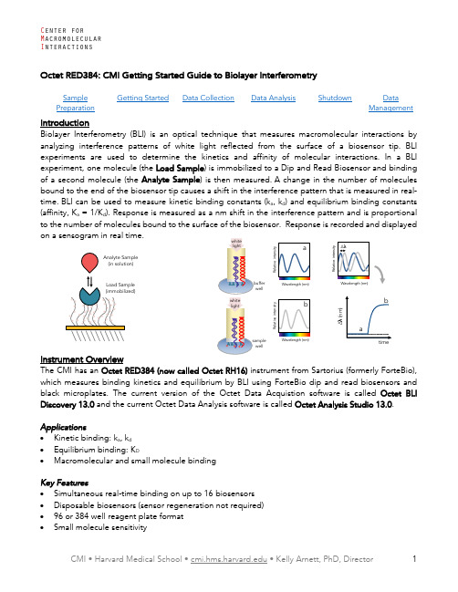
Data CollectionData AnalysisShutdownData Managementoptical technique that measures macromolecular interactions by white light reflected from the surface of a biosensor tip. BLI the kinetics and affinity of molecular interactions. In a BLI ) is immobilized to a Dip and Read Biosensor and binding ) is then measured. A change in the number of molecules a , k d ) and equilibrium binding constantsof the Octet Data Acquistion software is called Octet BLI Octet Analysis Studio 13.0.welllight welllight• ForteBio Biosensors.o See table below for popular sensor types and part numbers. Go to the Sartorius/ForteBiowebsite: https:///en/products/protein-analysis/octet-bli-detection/biosensors-chips-kits , for additional sensor types, including Anti-Mouse IgG Fc, Anti-Human Fab, Anti-GST, and biosensors recommended for quantitation.• At least two black microplates per experiment (one for soaking sensors and at least one forsamples and reagents).o Only Greiner Bio-One brand, black microplates or ForteBio plates are recommended (seetable below).• An empty biosensor tray to use as a working tray. • Pipettes (recommended). OCTET Black MicroplatesPart NumberGreiner Bio-One 96-well black flat-bottom PP, 200 µL 655209 (VWR 82050-784) Greiner Bio-One 384-well black flat-bottom PP, 80-120 µL 781209 (VWR 82051-318) ForteBio 384-well black tilted-bottom PP, 60 µL18-5080Sample PreparationAssay Buffers• Many buffers are compatible with BLI. It’s usually a good idea to start with a buffer system in whichyour proteins are well behaved.• Addition of 0.05% Tween 20 (or other surfactant) is usually required to prevent non-specificbinding, which is a frequent problem in BLI experiments.o Try detergent concentrations above the CMC, typically in the range of 0.02-0.1%.• The sample used for the association phase should be in a buffer identically matched to that usedfor the baseline and dissociation phase.o Buffer match is especially important when a buffer component has a high refractive index,such as DMSO. Immobilized load sample should also be in the same buffer, if possible.• 0.1% BSA can also be used to minimize non-specific binding.o ForteBio sells a detergent-based Kinetic Buffer (PBS + 0.02 % Tween20, 0.1 % BSA, 0.05 %sodium azide) that you might consider.o NOTE: BSA is not universally beneficial and can sometimes increase non-specific binding.Popular ForteBio Dip and Read Biosensors for Kinetics Part Number Streptavidin (SA) biosensors 18-5019 (96/tray) High Precision Streptavidin (SAX) biosensors 18-5117 High Precision Streptavidin (SAX2) biosensors 18-5136 Super-Streptavidin (SSA) biosensors (for small molecules) 18-5057 anti-His (HIS1K) biosensors 18-5120 Ni-NTA (NTA) biosensors 18-5101 Anti-Human IgG Fc biosensors 18-5010•All BLI experiments are setup with one molecule fixed to the biosensor surface (the Load Sample) and a second molecule in solution (the Analyte Sample).•Concentration should be accurately measuredo Errors in Load concentration can affect signal intensityo Errors in the Analyte concentration will directly translate to errors in the K D•Protein aggregates will interfere with BLI.o Filter or centrifuge samples before use.o Assess protein heterogeneity via light scattering.o Purify protein samples with soluble aggregates by size-exclusion chromatography. •Recommended concentration ranges:o Load Sample (immobilized) 10-50 µg/ml (~µM range)o Analyte 0.01 – 100 X K D (0.1 – 10 X K D)•Sample and Reagent plate well volumeo96-well 200 µlo384-well 80 – 120 µlo384-well tilted bottom 60 µlGetting StartedAn Octet experiment involves multiple steps in which ForteBio Dip and Read Biosensor are moved between wells in microplates containing buffers, reagents and samples. The instrument can hold up to 96 sensors (one tray) for use in experiments with multiple assays, each using up to 16 sensors. Reagents and samples are placed in 96- or 384-well black microplates. Plate 1 is used in all experiments and can hold any/all sample or reagent types. Plate 2 is an optional reagent plate that cannot hold analytes use in the association phase.timeReagent sequenceResourcesAdditional resources are available at the instrument, including Data Collection and Data Analysis software manuals.Experimental Design Tips•Do not overload the immobilized molecule.•The same well containing buffer should be used for the baseline and dissociation phase, assuming inter-step correction is performed.•For small molecule work, use Super-Streptavidin sensors and quench with biocytin (biotinyl-lysine at 10 µg/mL).•Use reference subtraction (there are several types).o Reference sample well has immobilized load sample and no analyte during association.o Reference sensor is a sensor to which no load sample is immobilized and is matched for analyte concentration.o Double Reference uses both reference well and reference sensor.•Experiments should be less than 3 hr (10 % volume loss ~ 3.5 hours at 30 ˚C).Data CollectionStartup1.Book time on the PPMS calendar before you start.2.Login to the computer using your PPMS credentials (eCommons ID and password).3.The instrument should generally be left powered on at all times.a.If it is not powered on, the power supply is on the shelf above the instrument.4.Design you experiment in the Data Acquisition software before setting up your sample and reagentplates.5.Open the instrument door with the Present Stage button in the software (green eject button). DoNOT pull on the thing that looks like a handle.Experimental Data Collection1.Start the Octet BLI Discovery Software (formerly Data Acquisition Software). The current version willbe on the Desktop (older versions are also usable and found in “older versions” folder).a.Wait for initialization.b.Select New Kinetics Experiment in the Experiment Wizard, or open a method file.c.The Experiment Wizard has 5 sections tabs to guide you through experimental setup.2.Plate Definition:a.Select data acquisition mode. Read Head: 16 channel or 8 channel.i)16 channel mode uses up to 16 sensors and moves in 2 column increments.ii)8 channel mode uses up to 8 sensors and can move in 1 column increments.b.To modify plate format, select Modify Plate:i)Choose either 96-well or 384-well format for Plate 1 and Plate 2CMI Getting Started Guide C enter forM acromolecular I nteractionsSelect a well or wells to define (shift-click to select all wells in column on 96-well or alternating wells on 384-well plate).c. Right-click to pull up Sample Type Menu and choose type for the selected wells.i) Select "Set Well Data" from the Sample Type Menu to add information or fill in the PlateData tables.ii) A molar concentration for the samples is required for fitting. iii) Required Reagent Types(1) Buffer (baseline before load) (2) Load Sample (load)(3) Mock Load Buffer (for reference sensor load step) (4) Buffer (baseline before association and dissociation)(5) Sample (association phase), use a range of concentrations, include 0 for reference sample iv) Optional Reagent Types(1) Quench (e.g. biocytin for blocking)(2) Regeneration solutions (for sensor reuse or serial data collection)v) Include a zero concentration of analyte (a reference sample well) to correct for a drift in thebaseline(1) Several sensor types have significant drift. (2) A reference sample well is required for NTA. vi) Test non-specific binding with Reference Sensors d. Fill your reagent plate(s) according to the plate map. 3. Assay Definition:a. Plate 1 and Plate 2 show plate layouts (step back to Plate Definition to modify).b. Create a list of steps in the Step Data List.i) Sample steps (s):(1) Baseline 120 (60 – 300) (2) Loading 120 (120 – 600) (3) (Quench) 60 (30 – 120) optional quench (eg. Biocytin on SA or SSA) (4) Association 300 (60 – 600) (5) Dissociation 600 (60 – 600+) ii) Shake speed 1,000 RPM.c. Create an assay (a group of ordered steps with plate information).i) Select a column from a plate and select a step in Step Data List. ii) Double-click or click Add… to add a step to Assay Step List. iii) Select the sensor type for the assay. iv) Typical assay order:(1) Baseline (2) Loading (3) Baseline (4) Association (5) Dissocation d. To create a new Assays, click New Assay or select all steps in Assay 1 and click replicate. Modifythe sample column as needed.A group of “Baseline – Assocation – Dissocation” steps are required for recognition as a binding assay and can be overlayedfor kinetic analysis. Don’t forget the baseline before association.CMI Getting Started GuideC enter forM acromolecular I nteractions 4. Sensor Assignment:a. This step tells you where to put sensors in the Sensor Tray.i) You should always check the box marked Replace sensors in tray after use . This will returnsensors to the tray after your experiment (and prevent them from clogging the instrument, as there is a design flaw in the sensor discard shoot).ii) Plate 1 (and 2) indicate wells that each sensor group will enter in an assay. iii) Sensor type should match those from the Assay Definition.b. Fill a sensor tray with sensors in the marked positions and place a 96-well plate underneath withsoaking buffer (usually running buffer) in the wells with sensors.5. Review Experiment:a. Click the arrow to review each assay step in your experiment. 6. Run Experiment:a. Assign a location for your data (choose your folder inside your lab folder).b. Enter the experiment run name (avoid using the default name Experiment_1).c. Set the Run Settings:i) Check all boxes except for “Present Stage at end of experiment” which should be uncheckedunless you will be present at the end of your experiment.ii) Set experiment delay for soaking and equilibration time (10 min). iii) Set temperature (30 ˚C minimum). d. Advanced Settings:i) Set Sensor Offset: 4 mm for standard well volumes (see table below for other offsets). ii) Set Acquisition Rate: Standard Kinetics (5Hz, avg by 20). e. Save method file if using later. f. Start Run by pressing Go button. 7. During Run:a. Watch data collection in real-time.b. Avoid skipping or extending steps, especially if performing an experiment with a second assay(such as a reference assay). Only assays with identical number of steps and duration of steps can be merged for subtractions or comparison.c. When data collection is complete, close the Data Acquisition software and go to Data Analysis.Table of Recommended sensor offsets by well volume (from Octet User Manual)CMI Getting Started GuideC enter forM acromolecular I nteractionsData AnalysisOverviewThe current version of Octet Data Analysis software is called Octet Analysis Studio 13.0. The legacy software, Data Analysis and Data Analysis HT, is still available for use in the “older versions” folder.Data Analysis Studio features:• Data from multiple plates and/or experiments can be combined into one analysis. • More flexible reference subtraction options are available for kinetic analysis. • Customizable report format.• Export Results as a single file (this was not available older Data Analysis HT versions).Data Analysis Protocols1. Open the Octet Analysis Studio Software.2. Select Data:a. Click Explore in the Icon Bar to view data folders.b. Drag an Octet data folder to the Experiment Builder.i) More than one data file can be combined into one analysis by dragging additional files intothe Overlay section (must have the same number of steps and step lengths). ii) Octet data can also be Appended to the beginning or end of a data set.(1) To combine data with different step sizes.(2) For experiments with steps performed in different files (such as immobilization andassociation performed as different experiments).3. Process Data:a. Click Preprocess from the Operations Section of the Icon Bar.b. Assign Reference Sensors (sensors to which no ligand is immobilized).i) Go to the Reference Sensor Tab.ii) Click on column number or drag to select the reference sensors. iii) Right click on selection.iv) Set Sensor Type to Reference Sensor (sensor icon will change to diamond). v) Right click on plate.vi) Go to Subtract Reference and choose subtraction method.(1) In Rows (selects a reference from the same row as the sample).vii) Scroll down to see multiple plates and repeat the subtraction for each plate.viii) Check the table at the bottom to see the sensor subtraction formula used for each sensor. c. Assign Reference Samples (samples with zero concentration of analyte).i) Go to Reference Sample Tab.ii) Click (or CTRL-click) to select well(s) for reference samples (zero concentration). iii) Right click on selection.iv) Set Reference to Reference Sample Wells. v) Right click on plate.vi) Go to Subtract Reference and choose subtraction method.vii) In columns (selects a reference well from the same column as the samples).CMI Getting Started GuideC enter forM acromolecular I nteractionsviii) Scroll down to see multiple plates and repeat for each plate. ix) Check the table to see the well subtraction formula for each sensor. d. Data Corrections:i) Go to Data Correction Tab.ii) Align the Y axis to the average of baseline step (default is the last 5 seconds of the baseline). iii) Inter-step correction.(1) This step corrects for system artifacts (optical artifacts from buffer mismatch, etc.). (2) Choose a step to align (try dissociation first).(3) The baseline before association and dissociation steps must be performed from the samewell of a sample plate.(4) Should not be performed with very fast on-rates as kinetic data may be lost.iv) Noise Filtering (Savitsky-Golay Filtering, smoothing function) is recommended but optional. e. Export Processed data by clicking on Processed Data in Export Section of the Icon Bar to exportdata in a csv format for graphing in other programs.4. Kinetic Analysis:a. Fitting Parameters:i) Click on Kinetics in the Operations section of the Icon Bar. ii) Choose Steps to Analyze: Association and Dissociation. iii) Choose Model: 1:1.iv) Select Global Fitting (full).v) Group by Sample ID (or other grouping scheme) when performing a parallel experiment. vi) Group by Sensor if all concentrations are measured on the same sensor (a serial experiment). b. Examine Fitted curves.c. Steady-State Analysis (Equilibrium Fit).i) Check to include or uncheck to exclude data from the table.ii) In Steady-state dialog, choose Response as the mode of analysis (when kinetic data reachessteady-state at each concentration).iii) Choose Region of Analysis by defining Average from X to X (time interval).(1) This should be a region of the association curve that has reached equilibrium (or steady-state).(2) Default is a five sec window, five seconds from the end of the association phase.(3) For viewing, go to the graph window in the bottom right corner and select the steady-state tab.d. Save the Excel Report (for a summary of the analysis) or create a custom reporte. Export Results as a single file or multiple files for re-graphing and/or analysis in 3rd party software.f. Processing parameters are autosaved in the HTSettings.efrdi) To restart with default/no settings, you may delete the HTSettings file and reopen. ii) Save As to save processing parameters in Extended ForteBio File format (*.efrd). iii) Click on Open Workspace from the Icon Bar to reopen saved processed data.CMI Getting Started GuideC enter forM acromolecular I nteractionsShutdown 1. Remove sensor tray and reagent plates from the instrument. 2. Close the Octet door.3. Discard used biosensors with tips.4. Return borrowed empty sensor trays to the drawer under the instrument.5. Clean up in and around the instrument.6. Close the control and analysis software.7. Logoff from PPMS!Data ManagementTechnology Biolayer Interferometry InstrumentOctet RH16 (Octet Red 384) Recommended Repository Generalist RepositoryData Collection SoftwareCurrent Version Octet BLI Discovery, Version 13.0 Data Files (Type, ~size) experiment folder (contents below) 5 MB/experiment data file .frd 80 KB/measurement method file .fmf 35-45 KB/experiment plate definitions .jpg 30-90 KB/plate assay image .jpg 30-90 KB/experiment preprocessed data.xslx 200 KB/experimentData Analysis SoftwareCurrent Version Octet Analysis Studio, Version 13.0Data Files (Type, ~size) HT SettingsReadable Exports results table .xslx 5-10 KBexport report.xslxBook time and Report Problems through the PPMS system: https:///hms-cmi• rates are based on booked and real time usageContact ***************.edu with questions.last edited: 2023-05-12。

Survey of clustering data mining techniques

A Survey of Clustering Data Mining TechniquesPavel BerkhinYahoo!,Inc.pberkhin@Summary.Clustering is the division of data into groups of similar objects.It dis-regards some details in exchange for data simpliﬁrmally,clustering can be viewed as data modeling concisely summarizing the data,and,therefore,it re-lates to many disciplines from statistics to numerical analysis.Clustering plays an important role in a broad range of applications,from information retrieval to CRM. Such applications usually deal with large datasets and many attributes.Exploration of such data is a subject of data mining.This survey concentrates on clustering algorithms from a data mining perspective.1IntroductionThe goal of this survey is to provide a comprehensive review of diﬀerent clus-tering techniques in data mining.Clustering is a division of data into groups of similar objects.Each group,called a cluster,consists of objects that are similar to one another and dissimilar to objects of other groups.When repre-senting data with fewer clusters necessarily loses certainﬁne details(akin to lossy data compression),but achieves simpliﬁcation.It represents many data objects by few clusters,and hence,it models data by its clusters.Data mod-eling puts clustering in a historical perspective rooted in mathematics,sta-tistics,and numerical analysis.From a machine learning perspective clusters correspond to hidden patterns,the search for clusters is unsupervised learn-ing,and the resulting system represents a data concept.Therefore,clustering is unsupervised learning of a hidden data concept.Data mining applications add to a general picture three complications:(a)large databases,(b)many attributes,(c)attributes of diﬀerent types.This imposes on a data analysis se-vere computational requirements.Data mining applications include scientiﬁc data exploration,information retrieval,text mining,spatial databases,Web analysis,CRM,marketing,medical diagnostics,computational biology,and many others.They present real challenges to classic clustering algorithms. These challenges led to the emergence of powerful broadly applicable data2Pavel Berkhinmining clustering methods developed on the foundation of classic techniques.They are subject of this survey.1.1NotationsTo ﬁx the context and clarify terminology,consider a dataset X consisting of data points (i.e.,objects ,instances ,cases ,patterns ,tuples ,transactions )x i =(x i 1,···,x id ),i =1:N ,in attribute space A ,where each component x il ∈A l ,l =1:d ,is a numerical or nominal categorical attribute (i.e.,feature ,variable ,dimension ,component ,ﬁeld ).For a discussion of attribute data types see [106].Such point-by-attribute data format conceptually corresponds to a N ×d matrix and is used by a majority of algorithms reviewed below.However,data of other formats,such as variable length sequences and heterogeneous data,are not uncommon.The simplest subset in an attribute space is a direct Cartesian product of sub-ranges C = C l ⊂A ,C l ⊂A l ,called a segment (i.e.,cube ,cell ,region ).A unit is an elementary segment whose sub-ranges consist of a single category value,or of a small numerical bin.Describing the numbers of data points per every unit represents an extreme case of clustering,a histogram .This is a very expensive representation,and not a very revealing er driven segmentation is another commonly used practice in data exploration that utilizes expert knowledge regarding the importance of certain sub-domains.Unlike segmentation,clustering is assumed to be automatic,and so it is a machine learning technique.The ultimate goal of clustering is to assign points to a ﬁnite system of k subsets (clusters).Usually (but not always)subsets do not intersect,and their union is equal to a full dataset with the possible exception of outliersX =C 1 ··· C k C outliers ,C i C j =0,i =j.1.2Clustering Bibliography at GlanceGeneral references regarding clustering include [110],[205],[116],[131],[63],[72],[165],[119],[75],[141],[107],[91].A very good introduction to contem-porary data mining clustering techniques can be found in the textbook [106].There is a close relationship between clustering and many other ﬁelds.Clustering has always been used in statistics [10]and science [158].The clas-sic introduction into pattern recognition framework is given in [64].Typical applications include speech and character recognition.Machine learning clus-tering algorithms were applied to image segmentation and computer vision[117].For statistical approaches to pattern recognition see [56]and [85].Clus-tering can be viewed as a density estimation problem.This is the subject of traditional multivariate statistical estimation [197].Clustering is also widelyA Survey of Clustering Data Mining Techniques3 used for data compression in image processing,which is also known as vec-tor quantization[89].Dataﬁtting in numerical analysis provides still another venue in data modeling[53].This survey’s emphasis is on clustering in data mining.Such clustering is characterized by large datasets with many attributes of diﬀerent types. Though we do not even try to review particular applications,many important ideas are related to the speciﬁcﬁelds.Clustering in data mining was brought to life by intense developments in information retrieval and text mining[52], [206],[58],spatial database applications,for example,GIS or astronomical data,[223],[189],[68],sequence and heterogeneous data analysis[43],Web applications[48],[111],[81],DNA analysis in computational biology[23],and many others.They resulted in a large amount of application-speciﬁc devel-opments,but also in some general techniques.These techniques and classic clustering algorithms that relate to them are surveyed below.1.3Plan of Further PresentationClassiﬁcation of clustering algorithms is neither straightforward,nor canoni-cal.In reality,diﬀerent classes of algorithms overlap.Traditionally clustering techniques are broadly divided in hierarchical and partitioning.Hierarchical clustering is further subdivided into agglomerative and divisive.The basics of hierarchical clustering include Lance-Williams formula,idea of conceptual clustering,now classic algorithms SLINK,COBWEB,as well as newer algo-rithms CURE and CHAMELEON.We survey these algorithms in the section Hierarchical Clustering.While hierarchical algorithms gradually(dis)assemble points into clusters (as crystals grow),partitioning algorithms learn clusters directly.In doing so they try to discover clusters either by iteratively relocating points between subsets,or by identifying areas heavily populated with data.Algorithms of theﬁrst kind are called Partitioning Relocation Clustering. They are further classiﬁed into probabilistic clustering(EM framework,al-gorithms SNOB,AUTOCLASS,MCLUST),k-medoids methods(algorithms PAM,CLARA,CLARANS,and its extension),and k-means methods(diﬀer-ent schemes,initialization,optimization,harmonic means,extensions).Such methods concentrate on how well pointsﬁt into their clusters and tend to build clusters of proper convex shapes.Partitioning algorithms of the second type are surveyed in the section Density-Based Partitioning.They attempt to discover dense connected com-ponents of data,which areﬂexible in terms of their shape.Density-based connectivity is used in the algorithms DBSCAN,OPTICS,DBCLASD,while the algorithm DENCLUE exploits space density functions.These algorithms are less sensitive to outliers and can discover clusters of irregular shape.They usually work with low-dimensional numerical data,known as spatial data. Spatial objects could include not only points,but also geometrically extended objects(algorithm GDBSCAN).4Pavel BerkhinSome algorithms work with data indirectly by constructing summaries of data over the attribute space subsets.They perform space segmentation and then aggregate appropriate segments.We discuss them in the section Grid-Based Methods.They frequently use hierarchical agglomeration as one phase of processing.Algorithms BANG,STING,WaveCluster,and FC are discussed in this section.Grid-based methods are fast and handle outliers well.Grid-based methodology is also used as an intermediate step in many other algorithms (for example,CLIQUE,MAFIA).Categorical data is intimately connected with transactional databases.The concept of a similarity alone is not suﬃcient for clustering such data.The idea of categorical data co-occurrence comes to the rescue.The algorithms ROCK,SNN,and CACTUS are surveyed in the section Co-Occurrence of Categorical Data.The situation gets even more aggravated with the growth of the number of items involved.To help with this problem the eﬀort is shifted from data clustering to pre-clustering of items or categorical attribute values. Development based on hyper-graph partitioning and the algorithm STIRR exemplify this approach.Many other clustering techniques are developed,primarily in machine learning,that either have theoretical signiﬁcance,are used traditionally out-side the data mining community,or do notﬁt in previously outlined categories. The boundary is blurred.In the section Other Developments we discuss the emerging direction of constraint-based clustering,the important researchﬁeld of graph partitioning,and the relationship of clustering to supervised learning, gradient descent,artiﬁcial neural networks,and evolutionary methods.Data Mining primarily works with large databases.Clustering large datasets presents scalability problems reviewed in the section Scalability and VLDB Extensions.Here we talk about algorithms like DIGNET,about BIRCH and other data squashing techniques,and about Hoﬀding or Chernoﬀbounds.Another trait of real-life data is high dimensionality.Corresponding de-velopments are surveyed in the section Clustering High Dimensional Data. The trouble comes from a decrease in metric separation when the dimension grows.One approach to dimensionality reduction uses attributes transforma-tions(DFT,PCA,wavelets).Another way to address the problem is through subspace clustering(algorithms CLIQUE,MAFIA,ENCLUS,OPTIGRID, PROCLUS,ORCLUS).Still another approach clusters attributes in groups and uses their derived proxies to cluster objects.This double clustering is known as co-clustering.Issues common to diﬀerent clustering methods are overviewed in the sec-tion General Algorithmic Issues.We talk about assessment of results,de-termination of appropriate number of clusters to build,data preprocessing, proximity measures,and handling of outliers.For reader’s convenience we provide a classiﬁcation of clustering algorithms closely followed by this survey:•Hierarchical MethodsA Survey of Clustering Data Mining Techniques5Agglomerative AlgorithmsDivisive Algorithms•Partitioning Relocation MethodsProbabilistic ClusteringK-medoids MethodsK-means Methods•Density-Based Partitioning MethodsDensity-Based Connectivity ClusteringDensity Functions Clustering•Grid-Based Methods•Methods Based on Co-Occurrence of Categorical Data•Other Clustering TechniquesConstraint-Based ClusteringGraph PartitioningClustering Algorithms and Supervised LearningClustering Algorithms in Machine Learning•Scalable Clustering Algorithms•Algorithms For High Dimensional DataSubspace ClusteringCo-Clustering Techniques1.4Important IssuesThe properties of clustering algorithms we are primarily concerned with in data mining include:•Type of attributes algorithm can handle•Scalability to large datasets•Ability to work with high dimensional data•Ability toﬁnd clusters of irregular shape•Handling outliers•Time complexity(we frequently simply use the term complexity)•Data order dependency•Labeling or assignment(hard or strict vs.soft or fuzzy)•Reliance on a priori knowledge and user deﬁned parameters •Interpretability of resultsRealistically,with every algorithm we discuss only some of these properties. The list is in no way exhaustive.For example,as appropriate,we also discuss algorithms ability to work in pre-deﬁned memory buﬀer,to restart,and to provide an intermediate solution.6Pavel Berkhin2Hierarchical ClusteringHierarchical clustering builds a cluster hierarchy or a tree of clusters,also known as a dendrogram.Every cluster node contains child clusters;sibling clusters partition the points covered by their common parent.Such an ap-proach allows exploring data on diﬀerent levels of granularity.Hierarchical clustering methods are categorized into agglomerative(bottom-up)and divi-sive(top-down)[116],[131].An agglomerative clustering starts with one-point (singleton)clusters and recursively merges two or more of the most similar clusters.A divisive clustering starts with a single cluster containing all data points and recursively splits the most appropriate cluster.The process contin-ues until a stopping criterion(frequently,the requested number k of clusters) is achieved.Advantages of hierarchical clustering include:•Flexibility regarding the level of granularity•Ease of handling any form of similarity or distance•Applicability to any attribute typesDisadvantages of hierarchical clustering are related to:•Vagueness of termination criteria•Most hierarchical algorithms do not revisit(intermediate)clusters once constructed.The classic approaches to hierarchical clustering are presented in the sub-section Linkage Metrics.Hierarchical clustering based on linkage metrics re-sults in clusters of proper(convex)shapes.Active contemporary eﬀorts to build cluster systems that incorporate our intuitive concept of clusters as con-nected components of arbitrary shape,including the algorithms CURE and CHAMELEON,are surveyed in the subsection Hierarchical Clusters of Arbi-trary Shapes.Divisive techniques based on binary taxonomies are presented in the subsection Binary Divisive Partitioning.The subsection Other Devel-opments contains information related to incremental learning,model-based clustering,and cluster reﬁnement.In hierarchical clustering our regular point-by-attribute data representa-tion frequently is of secondary importance.Instead,hierarchical clustering frequently deals with the N×N matrix of distances(dissimilarities)or sim-ilarities between training points sometimes called a connectivity matrix.So-called linkage metrics are constructed from elements of this matrix.The re-quirement of keeping a connectivity matrix in memory is unrealistic.To relax this limitation diﬀerent techniques are used to sparsify(introduce zeros into) the connectivity matrix.This can be done by omitting entries smaller than a certain threshold,by using only a certain subset of data representatives,or by keeping with each point only a certain number of its nearest neighbors(for nearest neighbor chains see[177]).Notice that the way we process the original (dis)similarity matrix and construct a linkage metric reﬂects our a priori ideas about the data model.A Survey of Clustering Data Mining Techniques7With the(sparsiﬁed)connectivity matrix we can associate the weighted connectivity graph G(X,E)whose vertices X are data points,and edges E and their weights are deﬁned by the connectivity matrix.This establishes a connection between hierarchical clustering and graph partitioning.One of the most striking developments in hierarchical clustering is the algorithm BIRCH.It is discussed in the section Scalable VLDB Extensions.Hierarchical clustering initializes a cluster system as a set of singleton clusters(agglomerative case)or a single cluster of all points(divisive case) and proceeds iteratively merging or splitting the most appropriate cluster(s) until the stopping criterion is achieved.The appropriateness of a cluster(s) for merging or splitting depends on the(dis)similarity of cluster(s)elements. This reﬂects a general presumption that clusters consist of similar points.An important example of dissimilarity between two points is the distance between them.To merge or split subsets of points rather than individual points,the dis-tance between individual points has to be generalized to the distance between subsets.Such a derived proximity measure is called a linkage metric.The type of a linkage metric signiﬁcantly aﬀects hierarchical algorithms,because it re-ﬂects a particular concept of closeness and connectivity.Major inter-cluster linkage metrics[171],[177]include single link,average link,and complete link. The underlying dissimilarity measure(usually,distance)is computed for every pair of nodes with one node in theﬁrst set and another node in the second set.A speciﬁc operation such as minimum(single link),average(average link),or maximum(complete link)is applied to pair-wise dissimilarity measures:d(C1,C2)=Op{d(x,y),x∈C1,y∈C2}Early examples include the algorithm SLINK[199],which implements single link(Op=min),Voorhees’method[215],which implements average link (Op=Avr),and the algorithm CLINK[55],which implements complete link (Op=max).It is related to the problem ofﬁnding the Euclidean minimal spanning tree[224]and has O(N2)complexity.The methods using inter-cluster distances deﬁned in terms of pairs of nodes(one in each respective cluster)are called graph methods.They do not use any cluster representation other than a set of points.This name naturally relates to the connectivity graph G(X,E)introduced above,because every data partition corresponds to a graph partition.Such methods can be augmented by so-called geometric methods in which a cluster is represented by its central point.Under the assumption of numerical attributes,the center point is deﬁned as a centroid or an average of two cluster centroids subject to agglomeration.It results in centroid,median,and minimum variance linkage metrics.All of the above linkage metrics can be derived from the Lance-Williams updating formula[145],d(C iC j,C k)=a(i)d(C i,C k)+a(j)d(C j,C k)+b·d(C i,C j)+c|d(C i,C k)−d(C j,C k)|.8Pavel BerkhinHere a,b,c are coeﬃcients corresponding to a particular linkage.This formula expresses a linkage metric between a union of the two clusters and the third cluster in terms of underlying nodes.The Lance-Williams formula is crucial to making the dis(similarity)computations feasible.Surveys of linkage metrics can be found in [170][54].When distance is used as a base measure,linkage metrics capture inter-cluster proximity.However,a similarity-based view that results in intra-cluster connectivity considerations is also used,for example,in the original average link agglomeration (Group-Average Method)[116].Under reasonable assumptions,such as reducibility condition (graph meth-ods satisfy this condition),linkage metrics methods suﬀer from O N 2 time complexity [177].Despite the unfavorable time complexity,these algorithms are widely used.As an example,the algorithm AGNES (AGlomerative NESt-ing)[131]is used in S-Plus.When the connectivity N ×N matrix is sparsiﬁed,graph methods directly dealing with the connectivity graph G can be used.In particular,hierarchical divisive MST (Minimum Spanning Tree)algorithm is based on graph parti-tioning [116].2.1Hierarchical Clusters of Arbitrary ShapesFor spatial data,linkage metrics based on Euclidean distance naturally gener-ate clusters of convex shapes.Meanwhile,visual inspection of spatial images frequently discovers clusters with curvy appearance.Guha et al.[99]introduced the hierarchical agglomerative clustering algo-rithm CURE (Clustering Using REpresentatives).This algorithm has a num-ber of novel features of general importance.It takes special steps to handle outliers and to provide labeling in assignment stage.It also uses two techniques to achieve scalability:data sampling (section 8),and data partitioning.CURE creates p partitions,so that ﬁne granularity clusters are constructed in parti-tions ﬁrst.A major feature of CURE is that it represents a cluster by a ﬁxed number,c ,of points scattered around it.The distance between two clusters used in the agglomerative process is the minimum of distances between two scattered representatives.Therefore,CURE takes a middle approach between the graph (all-points)methods and the geometric (one centroid)methods.Single and average link closeness are replaced by representatives’aggregate closeness.Selecting representatives scattered around a cluster makes it pos-sible to cover non-spherical shapes.As before,agglomeration continues until the requested number k of clusters is achieved.CURE employs one additional trick:originally selected scattered points are shrunk to the geometric centroid of the cluster by a user-speciﬁed factor α.Shrinkage suppresses the aﬀect of outliers;outliers happen to be located further from the cluster centroid than the other scattered representatives.CURE is capable of ﬁnding clusters of diﬀerent shapes and sizes,and it is insensitive to outliers.Because CURE uses sampling,estimation of its complexity is not straightforward.For low-dimensional data authors provide a complexity estimate of O (N 2sample )deﬁnedA Survey of Clustering Data Mining Techniques9 in terms of a sample size.More exact bounds depend on input parameters: shrink factorα,number of representative points c,number of partitions p,and a sample size.Figure1(a)illustrates agglomeration in CURE.Three clusters, each with three representatives,are shown before and after the merge and shrinkage.Two closest representatives are connected.While the algorithm CURE works with numerical attributes(particularly low dimensional spatial data),the algorithm ROCK developed by the same researchers[100]targets hierarchical agglomerative clustering for categorical attributes.It is reviewed in the section Co-Occurrence of Categorical Data.The hierarchical agglomerative algorithm CHAMELEON[127]uses the connectivity graph G corresponding to the K-nearest neighbor model spar-siﬁcation of the connectivity matrix:the edges of K most similar points to any given point are preserved,the rest are pruned.CHAMELEON has two stages.In theﬁrst stage small tight clusters are built to ignite the second stage.This involves a graph partitioning[129].In the second stage agglomer-ative process is performed.It utilizes measures of relative inter-connectivity RI(C i,C j)and relative closeness RC(C i,C j);both are locally normalized by internal interconnectivity and closeness of clusters C i and C j.In this sense the modeling is dynamic:it depends on data locally.Normalization involves certain non-obvious graph operations[129].CHAMELEON relies heavily on graph partitioning implemented in the library HMETIS(see the section6). Agglomerative process depends on user provided thresholds.A decision to merge is made based on the combinationRI(C i,C j)·RC(C i,C j)αof local measures.The algorithm does not depend on assumptions about the data model.It has been proven toﬁnd clusters of diﬀerent shapes,densities, and sizes in2D(two-dimensional)space.It has a complexity of O(Nm+ Nlog(N)+m2log(m),where m is the number of sub-clusters built during the ﬁrst initialization phase.Figure1(b)(analogous to the one in[127])clariﬁes the diﬀerence with CURE.It presents a choice of four clusters(a)-(d)for a merge.While CURE would merge clusters(a)and(b),CHAMELEON makes intuitively better choice of merging(c)and(d).2.2Binary Divisive PartitioningIn linguistics,information retrieval,and document clustering applications bi-nary taxonomies are very useful.Linear algebra methods,based on singular value decomposition(SVD)are used for this purpose in collaborativeﬁlter-ing and information retrieval[26].Application of SVD to hierarchical divisive clustering of document collections resulted in the PDDP(Principal Direction Divisive Partitioning)algorithm[31].In our notations,object x is a docu-ment,l th attribute corresponds to a word(index term),and a matrix X entry x il is a measure(e.g.TF-IDF)of l-term frequency in a document x.PDDP constructs SVD decomposition of the matrix10Pavel Berkhin(a)Algorithm CURE (b)Algorithm CHAMELEONFig.1.Agglomeration in Clusters of Arbitrary Shapes(X −e ¯x ),¯x =1Ni =1:N x i ,e =(1,...,1)T .This algorithm bisects data in Euclidean space by a hyperplane that passes through data centroid orthogonal to the eigenvector with the largest singular value.A k -way split is also possible if the k largest singular values are consid-ered.Bisecting is a good way to categorize documents and it yields a binary tree.When k -means (2-means)is used for bisecting,the dividing hyperplane is orthogonal to the line connecting the two centroids.The comparative study of SVD vs.k -means approaches [191]can be used for further references.Hier-archical divisive bisecting k -means was proven [206]to be preferable to PDDP for document clustering.While PDDP or 2-means are concerned with how to split a cluster,the problem of which cluster to split is also important.Simple strategies are:(1)split each node at a given level,(2)split the cluster with highest cardinality,and,(3)split the cluster with the largest intra-cluster variance.All three strategies have problems.For a more detailed analysis of this subject and better strategies,see [192].2.3Other DevelopmentsOne of early agglomerative clustering algorithms,Ward’s method [222],is based not on linkage metric,but on an objective function used in k -means.The merger decision is viewed in terms of its eﬀect on the objective function.The popular hierarchical clustering algorithm for categorical data COB-WEB [77]has two very important qualities.First,it utilizes incremental learn-ing.Instead of following divisive or agglomerative approaches,it dynamically builds a dendrogram by processing one data point at a time.Second,COB-WEB is an example of conceptual or model-based learning.This means that each cluster is considered as a model that can be described intrinsically,rather than as a collection of points assigned to it.COBWEB’s dendrogram is calleda classiﬁcation tree.Each tree node(cluster)C is associated with the condi-tional probabilities for categorical attribute-values pairs,P r(x l=νlp|C),l=1:d,p=1:|A l|.This easily can be recognized as a C-speciﬁc Na¨ıve Bayes classiﬁer.During the classiﬁcation tree construction,every new point is descended along the tree and the tree is potentially updated(by an insert/split/merge/create op-eration).Decisions are based on the category utility[49]CU{C1,...,C k}=1j=1:kCU(C j)CU(C j)=l,p(P r(x l=νlp|C j)2−(P r(x l=νlp)2.Category utility is similar to the GINI index.It rewards clusters C j for in-creases in predictability of the categorical attribute valuesνlp.Being incre-mental,COBWEB is fast with a complexity of O(tN),though it depends non-linearly on tree characteristics packed into a constant t.There is a similar incremental hierarchical algorithm for all numerical attributes called CLAS-SIT[88].CLASSIT associates normal distributions with cluster nodes.Both algorithms can result in highly unbalanced trees.Chiu et al.[47]proposed another conceptual or model-based approach to hierarchical clustering.This development contains several diﬀerent use-ful features,such as the extension of scalability preprocessing to categori-cal attributes,outliers handling,and a two-step strategy for monitoring the number of clusters including BIC(deﬁned below).A model associated with a cluster covers both numerical and categorical attributes and constitutes a blend of Gaussian and multinomial models.Denote corresponding multivari-ate parameters byθ.With every cluster C we associate a logarithm of its (classiﬁcation)likelihoodl C=x i∈Clog(p(x i|θ))The algorithm uses maximum likelihood estimates for parameterθ.The dis-tance between two clusters is deﬁned(instead of linkage metric)as a decrease in log-likelihoodd(C1,C2)=l C1+l C2−l C1∪C2caused by merging of the two clusters under consideration.The agglomerative process continues until the stopping criterion is satisﬁed.As such,determina-tion of the best k is automatic.This algorithm has the commercial implemen-tation(in SPSS Clementine).The complexity of the algorithm is linear in N for the summarization phase.Traditional hierarchical clustering does not change points membership in once assigned clusters due to its greedy approach:after a merge or a split is selected it is not reﬁned.Though COBWEB does reconsider its decisions,its。

1、下载文档前请自行甄别文档内容的完整性，平台不提供额外的编辑、内容补充、找答案等附加服务。
2、"仅部分预览"的文档,不可在线预览部分如存在完整性等问题,可反馈申请退款(可完整预览的文档不适用该条件!)。
3、如文档侵犯您的权益，请联系客服反馈,我们会尽快为您处理(人工客服工作时间：9:00-18:30)。

Working Load Stock Weight Limit No. Each (t)* S-209T (kg) 1 2 1018706 1018742 .14 .17 .33 .62 1.07 1-1/2 1018724 3-1/4 1018760 4-3/4 1018778
Dimensions (mm) A B C D E F G H L M P
3-1/4 1018760 1.37 4-3/4 1018778 2.35
1.06 .75 2.38 .63 1.69 1.50 2.94 4.19 .44 3.34 .69 1.25 .88 2.81 .75 2.00 1.81 3.50 4.97 .50 3.97 .81
Байду номын сангаас
Nominal Size (in.) 3/8 7/16 1/2 5/8 3/4
• •
CROSBY PRODUCTS DISTRIBUTED BY:
Imperial / Metric
New S-209T Theatrical Shackle
Working Nominal Load Stock Weight Size Limit No. Each (in.) (t)* S-209T (lbs.) 3/8 7/16 1/2 5/8 3/4 1 2 1018706 1018742 .31 .38 .72 1-1/2 1018724
*NOTE: Maximum Proof Load is 2.0 times the Working Load Limit. Minimum Ultimate Strength is 6 times the Working Load Limit. For Working Load Limit reduction due to side loading applications, see the Crosby General Catalog. Crosby U.S.A. P.O. Box 3128 Tulsa, OK 74101 U.S.A. Sales Office: (918) 834-4611 FAX: (918) 832-0940 crosbygroup@
9992014
Crosby Canada 145 Heart Lake Road Brampton, Ontario, L6W 3K3 Canada Sales Office: (905) 451-9261 FAX (877) 260-5106 sales@crosby.ca
Crosby Europe Industriepark Zone B nr 26 B-2220 Heist-op-den-Berg Belgium Sales Office: 32-15-757125 FAX : 32-15-753764 sales@
Dimensions (in.) A .66 .75 .81 B C D E F G H L M P
Tolerance +/C .13 .13 .13 .13 .25 A .06 .06 .06 .06 .06
.44 1.44 .38 1.03 .91 1.78 2.49 .25 2.02 .38 .50 1.69 .44 1.16 1.06 2.03 2.91 .31 2.37 .44 .63 1.88 .50 1.31 1.19 2.31 3.28 .38 2.69 .50
New S-209T Theatrical Shackle
Same Dependability and Durability with a new finish . . .
• • • • • • • • Sizes: 3/8” through 3/4”. Capacities: 1 through 4-3/4 metric tonnes. Forged - Quenched and Tempered, with alloy pins. Working Load Limit permanently shown on every shackle. Flat black baked on powder coat finish. Fatigue Rated. Industry leading 6 to 1 design factor. Screw pin anchor shackles meet the performance requirement of Federal Specification RR-C-271D Type IV A, Grade a, Class 2, except for those provisions required of the contractor. Meets the performance requirements of EN13889:2003. Crosby products meet or exceed all requirements of ASME B30.26 including identification, ductility, design factor, proof load and temperature requirements. Importantly, Crosby products meet other critical performance requirements including fatigue life, impact properties and material traceability, not addressed by ASME B30.26.
Tolerance +/C A
16.8 11.2 36.6 9.65 26.2 23.1 45.2 63.0 6.35 51.5 9.65 3.30 1.50 19.1 12.7 42.9 11.2 29.5 26.9 51.5 74.0 7.85 60.5 11.2 3.30 1.50 20.6 16.0 47.8 12.7 33.3 30.2 58.5 83.5 9.65 68.5 12.7 3.30 1.50 26.9 19.1 60.5 16.0 42.9 38.1 74.5 106 11.2 85.0 17.5 6.35 1.50 31.8 22.4 71.5 19.1 51.0 46.0 89.0 126 12.7 101 20.6 6.35 1.50