discrete-time (3)
英语跨文化交际案例分析

Encounter (1)
U1 The Taxi (P.1)
1. Maybe the taxi driver is trying to cheat Lee. 2. Perhaps there are extra charges for luggage that Lee doesn’t know about. 3. It may be that the driver has included a tip for himself, perhaps because he knows Lee is a foreigner and thinks she doesn’t know that she should tip. 4. One possibility is that there are extra charges for tolls (过路费) that Lee doesn’t know about. 5. It is possible that there is something wrong with the meter, or fares (车费) have recently gone up and the meter hasn’t been adjusted yet.
4. Ms. Kelsen may feel that she only did her duty, so she has done nothing to deserve such a special gift. 5. Ms. Kelsen may feel uncomfortable because she assumes Frank cannot afford to give expensive gifts. 6. Ms. Kelsen may feel that accepting the gift would put her under obligation to Frank. (Most Westerners feel that accepting a valuable gift entails a degree of reciprocity(酬答) .
奥本海姆版信号与系统ppt
+
Energy : t1 t t2
2
1
shift
f (t )
2 1
1 t
2
2
0
Scaling
Scaling
2
reversal
t
f (t )
2 1
shift
2 1
f (1 t )
f (1 3t )
1
t
0 1
1 0
1
2
2
1
0 1
t
1
2
1 3
0 2
t
3
f (3t )
f (1 3t )
Scaling
1
1 3
2
shift
1.2 Transformation of the Independent Variable
1.2.1 Examples of Transformations 1. Time Shift x(t-t0), x[n-n0]
t0<0
Advance
Time Shift
n0>0
Delay
x(t) and x(t-t0), or x[n] and x[n-n0]:
2. Time Reversal x(-t), x[-n]
——Reflection of x(t) or x[n]
2. Time Reversal x(-t), x[-n]
discrete-time (2)

8
Solution I of the difference equation —— Iteration method
Solution
e( k 2) 6e( k 1) 8e( k ) 1( k ) (k 0) e( k ) 0 e( k 2) 6e( k 1) 8e( k ) 1( k )
c(t ) r (0) g (t ) r (T ) g[t T ] r (nT ) g[t nT ]
c(kT ) r (0) g (kT ) r (T ) g[(k 1)T ] r (nT ) g[(k n)T ]
r (nT ) g[(k n)T ]
Tips:
Inverse Z-transform can only provide discrete-time signal x*(t), instead of continuous signal x(t)。
E(z) z
Long Division(长除法) Partial-Fraction expansion Expansion of Residue(留数法)
(3) To solve difference equations:
Iteration method Z-transform method
7
Example 1 The differential equation of a continuous system is:
( t ) 4e ( t ) 3e( t ) r ( t ) 1( t ) e (t 0)
n 1 k Lead Z e( t nT ) z E ( z ) e( kT ) z k 0 n
momentic类型 -回复

momentic类型-回复什么是momentic类型?momentic(即片刻)类型是一种注重记录和分享瞬间美好时刻的编程技术。
它通过使用中括号内的内容作为主题来编写文章,逐步展开讨论和回答相关问题。
这种类型的文章旨在帮助读者更好地理解和掌握这一主题,并为读者提供实用和丰富的信息。
篇幅:1500-2000字1. 引言(100-200字)momentic类型旨在捕捉和分享人们生活中的美好片刻。
在这个快节奏的世界中,我们经常忽略了那些逝去的瞬间。
本文将深入探讨momentic 类型,以中括号内的内容为主题,为读者提供全面的回答。
2. 什么是momentic类型(200-300字)momentic是一种注重记录和分享瞬间美好时刻的编程技术。
它能帮助我们在代码中捕捉和保存一段时刻,并在需要时回放这些时刻,以便更好地理解和分析程序的运行。
通过使用中括号内的内容作为主题,momentic 类型的文章可以一步一步回答问题,并提供详实而有趣的解释。
3. 为什么momentic类型重要(200-300字)momentic类型对于开发人员来说非常重要。
它使我们能够更好地理解程序的执行流程,帮助我们在复杂的代码中找出问题并进行调试。
此外,momentic类型还能帮助我们记录和分享瞬间美好时刻,增强开发人员之间的互动和交流。
4. 如何在momentic类型中记录瞬间时刻(300-400字)在momentic类型中,我们可以使用特定的函数或方法来记录瞬间时刻。
例如,我们可以使用`recordMoment()`函数来记录程序的某个关键时刻。
这个函数会将当前执行状态保存起来,包括变量的值和程序的执行位置。
我们还可以使用`playbackMoment()`函数来回放记录的时刻,以便重新执行代码和分析。
5. momentic类型的实际应用场景(400-500字)momentic类型在许多实际应用场景中有着重要的作用。
举例来说,当我们在开发一个复杂的机器学习模型时,我们可以使用momentic类型来记录模型在训练过程中的变化,以便更好地分析模型的性能和调整参数。
Chapter 3 Discrete-Time Fourier Transform
18
Note: X(ej) = | X(ej) |ej(+2k) = | X(ej) |ej()
7
3.1.1 The Definition
The definition of CTFT is:
X a ( j)
xa
(t
)e
jt
dt
The CTFT often is referred to as the Fourier spectrum.
The I-CTFT(inverse CTFT) is:
4
FS-continuous in time,discrete in frequency
1
X ( jk0 ) T0
T0 / 2 x(t )e jk0t dt
T0 / 2
x(t)
X ( jk 0 )e jk0t
k
Where:
x(t)
0
2F
2
T0
X ( jk0 )
T0
0
2
T0
5
Result:
to the following range of values: - ()
called the principal value.
19
20
The DTFTs of some sequences exhibit discontinuities of 2 in their phase responses. An alternate type of phase function that is a continuous function of is often used. It is derived from the original phase function by removing the discontinuities of 2.
simulink模块的分类及用途解析

simulink模块的分类及用途Commsim 2001 Education模块化通信仿真软件产品编号:808-110(单),112(10),115(25)Commsim 2001是一个理想的通信系统的教学软件。
它很适用于如‘信号与系统’、‘通信’、‘网络’等课程,难度适合从一般介绍到高级。
使学生学的更快并且掌握的更多。
Commsim2001含有200多个通用通信和数学模块,包含工业中的大部分编码器,调制器,滤波器,信号源,信道等,Commsim 2001中的模块和通常通信技术中的很一致,这可以确保你的学生学会当今所有最重要的通信技术。
要观察仿真的结果,你可以有多种选择:时域,频域,XY图,对数坐标,比特误码率,眼图和功率谱。
Scalable FunctionalityLike all other Electronics Workbench products Commsim 2001 is available in three tiers for the education community:Single: For use by professors/teachers in the creation of lectures, lessons, assignments etc Lab:For use by students in on-campus computer labsStudent: A special version for use by students on home PCs onlyHow Commsim is UsedCommsim 2001 is a powerful yet easy to use simulation tool that provides fast, accurate viewing of signals at any point in your system, via a natural sequence of steps. This power is presented to the user through an intuitive GUI(graphical User Interface) enabling drag and drop simplicity, just like all of the other products in the Electronics Workbench Family.Features at a Glance:∙Industry's Largest Library∙200+ Blocks∙Communication & Math Blocks∙Build your own Blocks/Models∙Drag and Drop Diagram Construction∙Analog, Digital & Mixed Systems∙Automatic Wiring∙Analog and Digital Modulators/Demodulators∙Wide variety of Encoders/Decoders∙Adaptive Equalizers∙Vector and Matrix Operations∙All popular Channel Models∙Filter Design Wizard and Response Viewer∙PLLs∙RF Elements and Accurate Distortion∙Complex Math∙Complex Envelope Representation∙Continuous, Discrete and Hybrid Simulation∙Autorestart and Single Step Algorithms∙Euler, Trapezoidal and Runge Kutta Integration Methods ∙Look-up Table Wizard∙Signal Probes∙Large variety of Plot Options∙Mathcad, Matlab OLE IntegrationPlacing and Connecting BlocksPlace desired blocks from the library by dragging and dropping(from either the menus or the toolbar) any of the over 200 functional blocks available. Once placed, connecting blocks is extremely straightforward-just click on one block's output then on other blocks input and Commsim takes care of the rest. Its that simple!You can also make use of hierarchical blocks to break up more complex systems, each of which can be assigned its own symbol.Blocks LibrariesThe science of understanding and teaching communication systems lies in being aware of a wide variety of "functional blocks" of technology available to "construct" the optimal transmitter or receiver, given a particular type of signal and channel.Commsim 2001 helps you to ensure your students learn all of today's most important communication technologies by delivering blocks to match all of the commonly used techniques in communications. The commsim library contains the industry's largest selection of coders, modulators, filters, sources, channels etc. You can even create your own blocks using equations or lower level functional blocks. Library BlocksBecause the right library is so essential to a good communications simulator, we have explained each family of blocks in detail. Simply click on the family to view more information.ChannelsEncoding/DecodingModulators/DemodulatorsOther Communication BlocksBasic BlocksChannelsModeling the medium through which a transmitted signal must pass is essential to accurately capture delay and distortion effects. Channels include copper wire, fiber, free space, etc.Channel Blocks Modeled in Commsim 2001∙Add.White Gaussian Noise (Complex & Real)∙Binary Symmetric Channel∙Jakes Mobile∙Multipath∙Propagation Loss∙Rice/Rayleigh Fading∙Rummler Multipath∙TWTAEncoding/DecodingSingle encoding is performed to increase the reliability of information transfer and can include companding and quantization (analog signals) or forward error correction (using convolutional or trellis cooling on digital signals).Commsim 2001 includes the following Encoders/Decoders∙Block Interleaver∙Convolutional Encoder∙Convolutional Interleaver∙Gray Decoder∙Gray Encoder∙Trellis Decoder∙Viterbi Decoder (Hard & Soft)Modulators/DemodulatorsCommsim provides the following analog and digital modulators/demodulation blocks, a subset of which use coherent methods(require phase synchronization in demodulation):Commsim 2001 includes the following Modulators/Demodulators∙AM∙DQPSK∙pi/4-DQPSK∙FM∙FSK∙I/Q∙MSK∙PM∙PAM (4,8)∙PPM∙PSK (2,4,8,16)∙QAM (16,32,64,256)∙SQPSK∙DQPSK∙pi/4-DQPSK Detector∙FM Demodulator∙PPM Demodulator∙PSK Detector (2,4,8,16)∙PAM Detector (2,4,8,16)∙QAM Detector (16,32,64,256)Other BlocksCommsim 2001 also provides many other communication blocks (filters, PLLs, digital etc.) and general mathematical functions (complex math, estimatio, etc.)Basic BlocksCommsim 2001 offers over 90 blocks for linear, non linear, continous, discrete-time, time varying, and hybrid system design.Basic Blocks Modeled in Commsim 2001∙Animation∙Annotation∙Arithmetic∙Boolean∙DDE∙Integration∙Linear Systems∙Matlab Interface∙Matrix Operations∙Nonlinear∙Optimization∙Random Generator∙Signal Consumer∙Signal Producer∙Time Delay∙TranscendentalCDMA通信系统的MATLAB仿真张广森,王虎(中国民航学院通信工程系,天津 300300)摘要:在简要介绍MATLAB语言的基础上,对使用MATLAB语言仿真的CDMA 通信系统进行描述。
1-Discrete-time+MPC+for+Beginners+
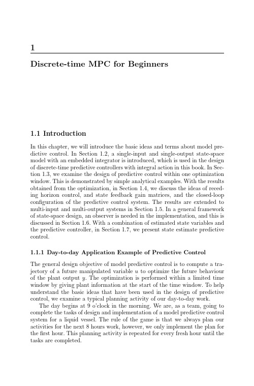
1Discrete-time MPC for Beginners1.1IntroductionIn this chapter,we will introduce the basic ideas and terms about model pre-dictive control.In Section1.2,a single-input and single-output state-space model with an embedded integrator is introduced,which is used in the design of discrete-time predictive controllers with integral action in this book.In Sec-tion1.3,we examine the design of predictive control within one optimization window.This is demonstrated by simple analytical examples.With the results obtained from the optimization,in Section1.4,we discuss the ideas of reced-ing horizon control,and state feedback gain matrices,and the closed-loop configuration of the predictive control system.The results are extended to multi-input and multi-output systems in Section1.5.In a general framework of state-space design,an observer is needed in the implementation,and this is discussed in Section1.6.With a combination of estimated state variables and the predictive controller,in Section1.7,we present state estimate predictive control.1.1.1Day-to-day Application Example of Predictive ControlThe general design objective of model predictive control is to compute a tra-jectory of a future manipulated variable u to optimize the future behaviour of the plant output y.The optimization is performed within a limited time window by giving plant information at the start of the time window.To help understand the basic ideas that have been used in the design of predictive control,we examine a typical planning activity of our day-to-day work.The day begins at9o’clock in the morning.We are,as a team,going to complete the tasks of design and implementation of a model predictive control system for a liquid vessel.The rule of the game is that we always plan our activities for the next8hours work,however,we only implement the plan for thefirst hour.This planning activity is repeated for every fresh hour until the tasks are completed.21Discrete-time MPC for BeginnersGiven the amount of background work that we have completed for9o’clock,we plan ahead for the next8hours.Assume that the work tasks are divided into modelling,design,simulation and pleting these tasks will be a function of various factors,such as how much effort we will put in,how well we will work as a team and whether we will get some additional help from others.These are the manipulated variables in the planning problem.Also,we have our limitations,such as our ability to understand the design problem,and whether we have good skills of computer hardware and software engineering. These are the hard and soft constraints in the planning.The background information we have already acquired is paramount for this planning work.After everything is considered,we determine the design tasks for the next 8hours as functions of the manipulated variables.Then we calculate hour-by-hour what we need to do in order to complete the tasks.In this calculation, based on the background information,we will take our limitations into con-sideration as the constraints,andfind the best way to achieve the goal.The end result of this planning gives us our projected activities from9o’clock to 5o’clock.Then we start working by implementing the activities for thefirst hour of our plan.At10o’clock,we check how much we have actually done for thefirst hour.This information is used for the planning of our next phase of activities. Maybe we have done less than we planned because we could not get the correct model or because one of the key members went for an emergency meeting.Nevertheless,at10o’clock,we make an assessment on what we have achieved,and use this updated information for planning our activities for the next8hours.Our objective may remain the same or may change.The length of time for the planning remains the same(8hours).We repeat the same planning process as it was at9o’clock,which then gives us the new projected activities for the next8hours.We implement thefirst hour of activities at 10o’clock.Again at11o’clock,we assess what we have achieved again and use the updated information for the plan of work for the next8hours.The planning and implementation process is repeated every hour until the original objective is achieved.There are three key elements required in the planning.Thefirst is the way of predicting what might happen(model);the second is the instrument of assessing our current activities(measurement);and the third is the instrument of implementing the planned activities(realization of control).The key issues in the planning exercise are:1.the time window for the planning isfixed at8hours;2.we need to know our current status before the planning;3.we take the best approach for the8hours work by taking the constraintsinto consideration,and the optimization is performed in real-time with a moving horizon time window and with the latest information available. The planning activity described here involves the principle of MPC.In this example,it is described by the terms that are to be used frequently in the1.1Introduction3 following:the moving horizon window,prediction horizon,receding horizon control,and control objective.They are introduced as below.1.Moving horizon window:the time-dependent window from an arbitrarytime t i to t i+T p.The length of the window T p remains constant.In this example,the planning activity is performed within an8-hour window, thus T p=8,with the measurement taken every hour.However,t i,which defines the beginning of the optimization window,increases on an hourly basis,starting with t i=9.2.Prediction horizon:dictates how‘far’we wish the future to be predictedfor.This parameter equals the length of the moving horizon window,T p.3.Receding horizon control:although the optimal trajectory of future controlsignal is completely described within the moving horizon window,the actual control input to the plant only takes thefirst sample of the control signal,while neglecting the rest of the trajectory.4.In the planning process,we need the information at time t i in order topredict the future.This information is denoted as x(t i)which is a vec-tor containing many relevant factors,and is either directly measured or estimated.5.A given model that will describe the dynamics of the system is paramountin predictive control.A good dynamic model will give a consistent and accurate prediction of the future.6.In order to make the best decision,a criterion is needed to reflect the ob-jective.The objective is related to an error function based on the difference between the desired and the actual responses.This objective function is often called the cost function J,and the optimal control action is found by minimizing this cost function within the optimization window.1.1.2Models Used in the DesignThere are three general approaches to predictive control design.Each ap-proach uses a unique model structure.In the earlier formulation of model predictive control,finite impulse response(FIR)models and step response models were favoured.FIR model/step response model based design algo-rithms include dynamic matrix control(DMC)(Cutler and Ramaker,1979) and the quadratic DMC formulation of Garcia and Morshedi(1986).The FIR type of models are appealing to process engineers because the model structure gives a transparent description of process time delay,response time and gain.However,they are limited to stable plants and often require large model orders.This model structure typically requires30to60impulse re-sponse coefficients depending on the process dynamics and choice of sampling intervals.Transfer function models give a more parsimonious description of process dynamics and are applicable to both stable and unstable plants.Rep-resentatives of transfer function model-based predictive control include the predictive control algorithm of Peterka(Peterka,1984)and the generalized41Discrete-time MPC for Beginnerspredictive control(GPC)algorithm of Clarke and colleagues(Clarke et al., 1987).The transfer function model-based predictive control is often considered to be less effective in handling multivariable plants.A state-space formulation of GPC has been presented in Ordys and Clarke(1993).Recent years have seen the growing popularity of predictive control de-sign using state-space design methods(Ricker,1991,Rawlings and Muske, 1993,Rawlings,2000,Maciejowski,2002).In this book,we will use state-space models,both in continuous time and discrete time for simplicity of the design framework and the direct link to the classical linear quadratic regulators. 1.2State-space Models with Embedded IntegratorModel predictive control systems are designed based on a mathematical model of the plant.The model to be used in the control system design is taken to be a state-space model.By using a state-space model,the current information required for predicting ahead is represented by the state variable at the current time.1.2.1Single-input and Single-output SystemFor simplicity,we begin our study by assuming that the underlying plant is a single-input and single-output system,described by:x m(k+1)=A m x m(k)+B m u(k),(1.1) y(k)=C m x m(k),(1.2)where u is the manipulated variable or input variable;y is the process output; and x m is the state variable vector with assumed dimension n1.Note that this plant model has u(k)as its input.Thus,we need to change the model to suit our design purpose in which an integrator is embedded.Note that a general formulation of a state-space model has a direct term from the input signal u(k)to the output y(k)asy(k)=C m x m(k)+D m u(k).However,due to the principle of receding horizon control,where a current information of the plant is required for prediction and control,we have im-plicitly assumed that the input u(k)cannot affect the output y(k)at the same time.Thus,D m=0in the plant model.Taking a difference operation on both sides of(1.1),we obtain thatx m(k+1)−x m(k)=A m(x m(k)−x m(k−1))+B m(u(k)−u(k−1)).1.2State-space Models with Embedded Integrator 5Let us denote the difference of the state variable byΔx m (k +1)=x m (k +1)−x m (k );Δx m (k )=x m (k )−x m (k −1),and the difference of the control variable byΔu (k )=u (k )−u (k −1).These are the increments of the variables x m (k )and u (k ).With this transfor-mation,the difference of the state-space equation is:Δx m (k +1)=A m Δx m (k )+B m Δu (k ).(1.3)Note that the input to the state-space model is Δu (k ).The next step is to connect Δx m (k )to the output y (k ).To do so,a new state variable vector is chosen to be x (k )= Δx m (k )T y (k ) T ,where superscript T indicates matrix transpose.Note thaty (k +1)−y (k )=C m (x m (k +1)−x m (k ))=C m Δx m (k +1)=C m A m Δx m (k )+C m B m Δu (k ).(1.4)Putting together (1.3)with (1.4)leads to the following state-space model:x (k +1) Δx m (k +1)y (k +1) =A A m o T m C m A m 1 x (k ) Δx m (k )y (k ) +B B m C m B mΔu (k )y (k )=C o m 1 Δx m (k )y (k ),(1.5)where o m =n 1 00...0 .The triplet (A,B,C )is called the augmented model,which will be used in the design of predictive control.Example 1.1.Consider a discrete-time model in the following form:x m (k +1)=A m x m (k )+B m u (k )y (k )=C m x m (k )(1.6)where the system matrices areA m = 1101 ;B m = 0.51;C m = 10 .Find the triplet matrices (A,B,C )in the augmented model (1.5)and calcu-late the eigenvalues of the system matrix,A ,of the augmented model.61Discrete-time MPC for BeginnersSolution.From (1.5),n 1=2and o m =[00].The augmented model for this plant is given byx (k +1)=Ax (k )+BΔu (k )y (k )=Cx (k ),(1.7)where the augmented system matrices are A = A m o T m C m A m 1 =⎡⎣110010111⎤⎦;B = B m C m B m =⎡⎣0.510.5⎤⎦;C = o m 1 = 001 .The characteristic equation of matrix A is given by ρ(λ)=det(λI −A )=det λI −A m o T m −C m A m (λ−1)=(λ−1)det(λI −A m )=(λ−1)3.(1.8)Therefore,the augmented state-space model has three eigenvalues at λ=1.Among them,two are from the original integrator plant,and one is from the augmentation of the plant model.1.2.2MATLAB Tutorial:Augmented Design ModelTutorial 1.1.The objective of this tutorial is to demonstrate how to obtain a discrete-time state-space model from a continuous-time state-space model,and form the augmented discrete-time state-space model.Consider a continuous-time system has the state-space model:˙x m (t )=⎡⎣010301010⎤⎦x m (t )+⎡⎣113⎤⎦u (t )y (t )= 010 x m (t ).(1.9)Step by Step1.Create a new file called extmodel.m.We form a continuous-time state vari-able model;then this continuous-time model is discretized using MATLAB function ‘c2dm’with specified sampling interval Δt .2.Enter the following program into the file:Ac =[010;301;010];Bc=[1;1;3];Cc=[010];Dc=zeros(1,1);Delta_t=1;[Ad,Bd,Cd,Dd]=c2dm(Ac,Bc,Cc,Dc,Delta_t);1.3Predictive Control within One Optimization Window7 3.The dimensions of the system matrices are determined to discover thenumbers of states,inputs and outputs.The augmented state-space model is produced.Continue entering the following program into thefile: [m1,n1]=size(Cd);[n1,n_in]=size(Bd);A_e=eye(n1+m1,n1+m1);A_e(1:n1,1:n1)=Ad;A_e(n1+1:n1+m1,1:n1)=Cd*Ad;B_e=zeros(n1+m1,n_in);B_e(1:n1,:)=Bd;B_e(n1+1:n1+m1,:)=Cd*Bd;C_e=zeros(m1,n1+m1);C_e(:,n1+1:n1+m1)=eye(m1,m1);4.Run this program to produce the augmented state variable model for thedesign of predictive control.1.3Predictive Control within One Optimization Window Upon formulation of the mathematical model,the next step in the design of a predictive control system is to calculate the predicted plant output with the future control signal as the adjustable variables.This prediction is described within an optimization window.This section will examine in detail the opti-mization carried out within this window.Here,we assume that the current time is k i and the length of the optimization window is N p as the number of samples.For simplicity,the case of single-input and single-output systems is consideredfirst,then the results are extended to multi-input and multi-output systems.1.3.1Prediction of State and Output VariablesAssuming that at the sampling instant k i,k i>0,the state variable vector x(k i)is available through measurement,the state x(k i)provides the current plant information.The more general situation where the state is not directly measured will be discussed later.The future control trajectory is denoted by Δu(k i),Δu(k i+1),...,Δu(k i+N c−1),where N c is called the control horizon dictating the number of parameters used to capture the future control trajectory.With given information x(k i), the future state variables are predicted for N p number of samples,where N p is called the prediction horizon.N p is also the length of the optimization window.We denote the future state variables asx(k i+1|k i),x(k i+2|k i),...,x(k i+m|k i),...,x(k i+N p|k i),81Discrete-time MPC for Beginnerswhere x (k i +m |k i )is the predicted state variable at k i +m with given current plant information x (k i ).The control horizon N c is chosen to be less than (or equal to)the prediction horizon N p .Based on the state-space model (A,B,C ),the future state variables are calculated sequentially using the set of future control parameters:x (k i +1|k i )=Ax (k i )+BΔu (k i )x (k i +2|k i )=Ax (k i +1|k i )+BΔu (k i +1)=A 2x (k i )+ABΔu (k i )+BΔu (k i +1)...x (k i +N p |k i )=A N p x (k i )+A N p −1BΔu (k i )+A N p −2BΔu (k i +1)+...+A N p −N c BΔu (k i +N c −1).From the predicted state variables,the predicted output variables are,by substitutiony (k i +1|k i )=CAx (k i )+CBΔu (k i )(1.10)y (k i +2|k i )=CA 2x (k i )+CABΔu (k i )+CBΔu (k i +1)y (k i +3|k i )=CA 3x (k i )+CA 2BΔu (k i )+CABΔu (k i +1)+CBΔu (k i +2)...y (k i +N p |k i )=CA N p x (k i )+CA N p −1BΔu (k i )+CA N p −2BΔu (k i +1)+...+CA N p −N c BΔu (k i +N c −1).(1.11)Note that all predicted variables are formulated in terms of current state variable information x (k i )and the future control movement Δu (k i +j ),where j =0,1,...N c −1.Define vectors Y = y (k i +1|k i )y (k i +2|k i )y (k i +3|k i )...y (k i +N p |k i )T ΔU = Δu (k i )Δu (k i +1)Δu (k i +2)...Δu (k i +N c −1) T ,where in the single-input and single-output case,the dimension of Y is N p and the dimension of ΔU is N c .We collect (1.10)and (1.11)together in a compact matrix form asY =F x (k i )+ΦΔU,(1.12)where F =⎡⎢⎢⎢⎢⎢⎣CACA 2CA 3...CA N p ⎤⎥⎥⎥⎥⎥⎦;Φ=⎡⎢⎢⎢⎢⎢⎣CB 00...0CAB CB 0...0CA 2B CAB CB ...0...CA N p −1B CA N p −2B CA N p −3B ...CA N p −N c B⎤⎥⎥⎥⎥⎥⎦.1.3Predictive Control within One Optimization Window9 1.3.2OptimizationFor a given set-point signal r(k i)at sample time k i,within a prediction horizon the objective of the predictive control system is to bring the predicted output as close as possible to the set-point signal,where we assume that the set-point signal remains constant in the optimization window.This objective is then translated into a design tofind the‘best’control parameter vectorΔU such that an error function between the set-point and the predicted output is minimized.Assuming that the data vector that contains the set-point information isR T s=N p11 (1)r(k i),we define the cost function J that reflects the control objective asJ=(R s−Y)T(R s−Y)+ΔU T¯RΔU,(1.13) where thefirst term is linked to the objective of minimizing the errors between the predicted output and the set-point signal while the second term reflects the consideration given to the size ofΔU when the objective function J is made to be as small as possible.¯R is a diagonal matrix in the form that¯R=rw I N c×N c(r w≥0)where r w is used as a tuning parameter for the desired closed-loop performance.For the case that r w=0,the cost function (1.13)is interpreted as the situation where we would not want to pay any attention to how large theΔU might be and our goal would be solely to make the error(R s−Y)T(R s−Y)as small as possible.For the case of large r w,the cost function(1.13)is interpreted as the situation where we would carefully consider how large theΔU might be and cautiously reduce the error (R s−Y)T(R s−Y).Tofind the optimalΔU that will minimize J,by using(1.12),J is ex-pressed asJ=(R s−F x(k i))T(R s−F x(k i))−2ΔU TΦT(R s−F x(k i))+ΔU T(ΦTΦ+¯R)ΔU.(1.14) From thefirst derivative of the cost function J:∂J∂ΔU=−2ΦT(R s−F x(k i))+2(ΦTΦ+¯R)ΔU,(1.15) the necessary condition of the minimum J is obtained as∂J∂ΔU=0,from which wefind the optimal solution for the control signal asΔU=(ΦTΦ+¯R)−1ΦT(R s−F x(k i)),(1.16)101Discrete-time MPC for Beginnerswith the assumption that (ΦT Φ+¯R)−1exists.The matrix (ΦT Φ+¯R )−1is called the Hessian matrix in the optimization literature.Note that R s is a data vector that contains the set-point information expressed asR s =N p [111...1]T r (k i )=¯Rs r (k i ),where¯Rs =N p [111...1]T .The optimal solution of the control signal is linked to the set-point signal r (k i )and the state variable x (k i )via the following equation:ΔU =(ΦT Φ+¯R )−1ΦT (¯R s r (k i )−F x (k i )).(1.17)Example 1.2.Suppose that a first-order system is described by the state equa-tion:x m (k +1)=ax m (k )+bu (k )y (k )=x m (k ),(1.18)where a =0.8and b =0.1are scalars.Find the augmented state-space model.Assuming a prediction horizon N p =10and control horizon N c =4,calcu-late the components that form the prediction of future output Y ,and the quantities ΦT Φ,ΦT F and ΦT ¯Rs .Assuming that at a time k i (k i =10for this example),r (k i )=1and the state vector x (k i )=[0.10.2]T ,find the optimal solution ΔU with respect to the cases where r w =0and r w =10,and compare the results.Solution.The augmented state-space equation is Δx m (k +1)y (k +1) = a 0a 1 Δx m (k )y (k ) + b b Δu (k )y (k )= 01 Δx m (k )y (k ).(1.19)Based on (1.12),the F and Φmatrices take the following forms:F =⎡⎢⎢⎢⎢⎢⎢⎢⎢⎢⎢⎢⎢⎢⎢⎣CA CA 2CA 3CA 4CA 5CA 6CA 7CA 8CA 9CA 10⎤⎥⎥⎥⎥⎥⎥⎥⎥⎥⎥⎥⎥⎥⎥⎦;Φ=⎡⎢⎢⎢⎢⎢⎢⎢⎢⎢⎢⎢⎢⎢⎢⎣CB 000CAB CB 00CA 2B CAB CB 0CA 3B CA 2B CAB CB CA 4B CA 3B CA 2B CAB CA 5B CA 4B CA 3B CA 2B CA 6B CA 5B CA 4B CA 3B CA 7B CA 6B CA 5B CA 4B CA 8B CA 7B CA 6B CA 5B CA 9B CA 8B CA 7B CA 6B ⎤⎥⎥⎥⎥⎥⎥⎥⎥⎥⎥⎥⎥⎥⎥⎦.1.3Predictive Control within One Optimization Window11 The coefficients in the F andΦmatrices are calculated as follows:CA=s11CA2=s21CA3=s31... CA k=s k1,(1.20)where s1=a,s2=a2+s1,...,s k=a k+s k−1,andCB=g0=bCAB=g1=ab+g0CA2B=g2=a2b+g1...CA k−1B=g k−1=a k−1b+g k−2CA k B=g k=a k b+g k−1.(1.21) With the plant parameters a=0.8and b=0.1,N p=10and N c=4,we calculate the quantitiesΦTΦ=⎡⎢⎢⎣1.15411.04070.91160.7726 1.04070.95490.84750.7259 0.91160.84750.76750.6674 0.77260.72590.66740.5943⎤⎥⎥⎦ΦT F=⎡⎢⎢⎣9.23253.21478.32592.76847.29272.33556.18111.9194⎤⎥⎥⎦;ΦT¯R s=⎡⎢⎢⎣3.21472.76842.33551.9194⎤⎥⎥⎦.Note that the vectorΦT¯R s is identical to the last column in the matrixΦT F. This is because the last column of F matrix is identical to¯R s.At time k i=10,the state vector x(k i)=[0.10.2]T.In thefirst case,the error between predicted Y and R s is reduced without any consideration to the magnitude of control ly,r w=0.Then,the optimalΔU is found through the calculationΔU=(ΦTΦ)−1(ΦT R s−ΦT F x(k i))=7.2−6.400T.We note that without weighting on the incremental control,the last two ele-mentsΔu(k i+2)=0andΔu(k i+3)=0,while thefirst two elements have a rather large magnitude.Figure1.1a shows the changes of the state variables where we can see that the predicted output y has reached the desired set-point121Discrete-time MPC for Beginners(a)State variables with no weight onΔu(b)State variables with weight on Δuparison of optimal solutions.Key:line (1)Δx m ;line (2)y 1while the Δx m decays to zero.To examine the effect of the weight r w on the optimal solution of the control,we let r w =10.The optimal solution of ΔU is given below,where I is a 4×4identity matrix,ΔU =(ΦT Φ+10×I )−1(ΦT R s −ΦT F x (k i ))(1.22)= 0.12690.10340.08290.065 T .With this choice,the magnitude of the first two control increments is signifi-cantly reduced,also the last two components are no longer zero.Figure 1.1b shows the optimal state variables.It is seen that the output y did not reach the set-point value of 1,however,the Δx m approaches zero.An observation follows from the comparison study.It seems that if we want the control to move cautiously,then it takes longer for the control signal to reach its steady state (i.e.,the values in ΔU decrease more slowly),because the optimal control energy is distributed over the longer period of future time.We can verify this by increasing N c to 9,while maintaining r w =10.The result shows that the magnitude of the elements in ΔU is reducing,but they are significant for the first 8elements:ΔU T = 0.12270.09930.07900.06140.04630.03340.02270.01390.0072 .In comparison with the case where N c =4,we note that when N c =9,the first four parameters in ΔU are slightly different from the previous case.Example 1.3.There is an alternative way to find the minimum of the cost function via completing the squares.This is an intuitive approach,also the minimum of the cost function becomes a by-product of the approach.Find the optimal solution for ΔU by completing the squares of the cost func-tion J (1.14).1.3Predictive Control within One Optimization Window 13Solution.From (1.14),by adding and subtracting the term(R s −F x (k i ))T Φ(ΦT Φ+¯R)−1ΦT (R s −F x (k i ))to the original cost function J ,its value remains unchanged.This leads toJ =(R s −F x (k i ))T (R s −F x (k i )) −2ΔU T ΦT (R s −F x (k i ))+ΔU T (ΦT Φ+¯R )ΔU + (R s −F x (k i ))T Φ(ΦT Φ+¯R)−1ΦT (R s −F x (k i ))−(R s −F x (k i ))T Φ(ΦT Φ+¯R)−1ΦT (R s −F x (k i )),(1.23)where the quantities under the .are the completed ‘squares’:J 0= ΔU −(ΦT Φ+¯R )−1ΦT (R s −F x (k i )) T ×(ΦT Φ+¯R ) ΔU −(ΦT Φ+¯R )−1ΦT (R s −F x (k i )) .(1.24)This can be easily verified by opening the squares.Since the first and last terms in (1.23)are independent of the variable ΔU (sometimes,we call this a decision variable),and (ΦT Φ+¯R)is assumed to be positive definite,then the minimum of the cost function J is achieved if the quantity J 0equals zero,i.e.,ΔU =(ΦT Φ+¯R)−1ΦT (R s −F x (k i )).(1.25)This is the optimal control solution.By substituting this optimal solution into the cost function (1.23),we obtain the minimum of the cost asJ min =(R s −F x (k i ))T (R s −F x (k i ))−(R s −F x (k i ))T Φ(ΦT Φ+¯R)−1ΦT (R s −F x (k i )).1.3.3MATLAB Tutorial:Computation of MPC GainsTutorial 1.2.The objective of this tutorial is to produce a MATLAB function for calculating ΦT Φ,ΦT F ,ΦT ¯Rs .The key here is to create F and Φmatrices.Φmatrix is a Toeplitz matrix,which is created by defining its first column,and the next column is obtained through shifting the previous column.Step by Step1.Create a new file called mpcgain.m.2.The first step is to create the augmented model for MPC design.The input parameters to the function are the state-space model (A p ,B p ,C p ),prediction horizon N p and control horizon N c .Enter the following program into the file:141Discrete-time MPC for Beginnersfunction[Phi_Phi,Phi_F,Phi_R,A_e,B_e,C_e]=mpcgain(Ap,Bp,Cp,Nc,Np);[m1,n1]=size(Cp);[n1,n_in]=size(Bp);A_e=eye(n1+m1,n1+m1);A_e(1:n1,1:n1)=Ap;A_e(n1+1:n1+m1,1:n1)=Cp*Ap;B_e=zeros(n1+m1,n_in);B_e(1:n1,:)=Bp;B_e(n1+1:n1+m1,:)=Cp*Bp;C_e=zeros(m1,n1+m1);C_e(:,n1+1:n1+m1)=eye(m1,m1);3.Note that the F and P hi matrices have special forms.By taking advantageof the special structure,we obtain the matrices.4.Continue entering the program into thefile:n=n1+m1;h(1,:)=C_e;F(1,:)=C_e*A_e;for kk=2:Nph(kk,:)=h(kk-1,:)*A_e;F(kk,:)=F(kk-1,:)*A_e;endv=h*B_e;Phi=zeros(Np,Nc);%declare the dimension of PhiPhi(:,1)=v;%first column of Phifor i=2:NcPhi(:,i)=[zeros(i-1,1);v(1:Np-i+1,1)];%Toeplitz matrixendBarRs=ones(Np,1);Phi_Phi=Phi’*Phi;Phi_F=Phi’*F;Phi_R=Phi’*BarRs;5.Type into the MATLAB Work Space with Ap=0.8,Bp=0.1,Cp=1,Nc=4and Np=10.Run this MATLAB function by typing[Phi_Phi,Phi_F,Phi_R,A_e,B_e,C_e]=mpcgain(Ap,Bp,Cp,Nc,Np);paring the results with the answers from Example1.2.If it is identicalto what was presented there,then your program is correct.7.Varying the prediction horizon and control horizon,observe the changesin these matrices.8.CalculateΔU by assuming the information of initial condition on x andr.The inverse of matrix M is calculated in MATLAB as inv(M).9.Validate the results in Example1.2.1.4Receding Horizon Control 151.4Receding Horizon ControlAlthough the optimal parameter vector ΔU contains the controls Δu (k i ),Δu (k i +1),Δu (k i +2),...,Δu (k i +N c −1),with the receding horizon control principle,we only implement the first sample of this sequence,i.e.,Δu (k i ),while ignoring the rest of the sequence.When the next sample period arrives,the more recent measurement is taken to form the state vector x (k i +1)for calculation of the new sequence of control signal.This procedure is repeated in real time to give the receding horizon control law.Example 1.4.We illustrate this procedure by continuing Example 1.2,where a first-order system with the state-space descriptionx m (k +1)=0.8x m (k )+0.1u (k )is used in the computation.We will consider the case r w =0.The initial conditions are x (10)=[0.10.2]T and u (9)=0.Solution.At sample time k i =10,the optimal control was previously com-puted as Δu (10)=7.2.Assuming that u (9)=0,then the control signal to the plant is u (10)=u (9)+Δu (10)=7.2and with x m (10)=y (10)=0.2,we calculate the next simulated plant state variablex m (11)=0.8x m (10)+0.1u (10)=0.88.(1.26)At k i =11,the new plant information is Δx m (11)=0.88−0.2=0.68and y (11)=0.88,which forms x (11)= 0.680.88 T .Then we obtainΔU =(ΦT Φ)−1(ΦT R s −ΦT F x (11))= −4.24−0.960.00000.0000 T .This leads to the optimal control u (11)=u (10)+Δu (11)=2.96.This new control is implemented to obtainx m (12)=0.8x m (11)+0.1u (11)=1.(1.27)At k i =12,the new plant information is Δx m (12)=1−0.88=0.12and y (12)=1,which forms x (12)= 0.121 .We obtainΔU =(ΦT Φ)−1(ΦT R s −ΦT F x (11))= −0.960.0000.00000.0000 T .This leads to the control at k i =12as u (12)=u (11)−0.96=2.By imple-menting this control,we obtain the next plant output asx m (13)=ax m (12)+bu (12)=1.(1.28)The new plant information is Δx m (13)=1−1=0and y (13)=1.From this information,we obtain。
Discrete-Time Integrator

Discrete-Time Integrator/p/1903691379执行离散时间信号的整合或累积即离散时间积分离散的离散时间积分器模块的功能您可以使用Discrete-Time Integrator模块,以取代Integrator块来创建一个纯粹的离散系统。
随着Discrete-Time Integrator块,您可以:•定义块对话框或输入到块的初始条件。
•定义输入增益(K)值。
•输出块的状态。
•定义的积分的上限和下限。
•复位状态,取决于一个额外的复位输入。
整合和积累方法该块可以整合或累积使用向前欧拉,向后欧拉,梯形方法。
假设u为输入,y是输出,x是的状态。
对于一个给定的步骤n,Simulink的更新y(n)和x(n+1)。
在积分模式中,T是块采样时间(ΔT的情况下,触发采样时间)。
在积累模式下,T = 1;块的采样时间确定时,计算输出,但不输出值。
K为增益值。
超出所值根据上限或下限剪辑。
•向前欧拉方法(默认),也被称为正向矩形,或左手逼近。
对于这种方法,1/s近似为T/(z-1).块的n步输出是由此产生的的表达式为:y(n) = y(n-1) + K*T*u(n-1)让x(n+1) = x(n) + K*T*u(n). 块使用以下步骤来计算其输出:步骤 0: y(0) = x(0) = IC (剪辑如果必要的)x(1) = y(0) + K*T*u(0)步骤 1: y(1) = x(1)x(2) = x(1) + K*T*u(1)步骤 n: y(n) = x(n)x(n+1) = x(n) + K*T*u(n) (剪辑如果必要的) 使用这种方法,输入端口1不具有直接馈通。
•向后Euler方法,也被称为向后矩形或近似右手。
对于这种方法,1/s近似为T*z/(z-1)块n步的输出是由此产生的的表达式为y(n) = y(n-1) + K*T*u(n)让x(n) = y(n-1). 块使用以下步骤来计算其输出步骤 0: y(0) = x(0) = IC (剪辑如果必要的)x(1) = y(0)或者,根据Use initial condition as initial and reset value for参数:步骤 0: x(0) = IC (剪辑如果必要的)x(1) = y(0) = x(0) + K*T*u(0)步骤 1: y(1) = x(1) + K*T*u(1)x(2) = y(1)步骤 n: y(n) = x(n) + K*T*u(n)x(n+1) = y(n)使用这种方法,输入端口1具有直接馈通。
- 1、下载文档前请自行甄别文档内容的完整性,平台不提供额外的编辑、内容补充、找答案等附加服务。
- 2、"仅部分预览"的文档,不可在线预览部分如存在完整性等问题,可反馈申请退款(可完整预览的文档不适用该条件!)。
- 3、如文档侵犯您的权益,请联系客服反馈,我们会尽快为您处理(人工客服工作时间:9:00-18:30)。
z ( w 1) ( w 1)
w 1 3 w 1 2 w 1 ) 119( ) 39 0 45( ) 117 ( w 1 w 1 w 1
(w 1)(w 1)2 39(w 1)3 0 D( w) 45( w 1)3 117( w 1)2 ( w 1) 119
Its characteristic function is:
1 G z 0
6
Necessary and Sufficient Condition for Stability of Linear Discrete-Time Systems ——All poles of (z) lie in the unit circle of z plane.
Prove:
M (z) Φ( z ) D( z )
(z ) (z
j 1 i 1 n i j
m
)
j 1
n
C jz zj
K (z)
c( k ) C j
j 1
n
k j
k
0
j 1
— Necessity — Sufficiency
n k c (t ) C j j ( t kT ) k 0 j 1
1 (1 z ) K Z 2 s ( s 1 )
1
( z 1) K 1 1 1 ( z 1) K Z 2 z s s s 1 z
14
Example 3 Consider the system shown in the figure (T=1). Determine the stable range of K. Routh criterion in w domain
1 e Ts K G( z) Z s s ( s 1 )
9
w-transformation and Routh criterion in w-domain
We find a transformation that maps the unit circle back onto the LHP while maintaining the algebraic structure of rational functions. A particular transformation that will accomplish this would be the bilinear transformation: Suppose
x2 y2 1 u ( x 1) 2 y 2
10
z 1 x 1 jy x2 1 y2 j2 y w u jv 2 2 z 1 x 1 jy ( x 1) y
2 2 x y 1 [w] imaginary axis u 0 0 2 2 ( x 1) y
7.5 Mathematical Models of Discrete-Time Systems
7.5.1 Linear Time-Invariant Difference Equations (1) Definition of difference (2) The difference equation and its solving method 7.5.2 Impulse-Transfer Function (1) Definition (2) Properties (3) Limitation (1) Switch between factors (2) No switch between factors (3) With ZOH (1) General Method (2) Mason’s formula
1
① Forward ① Iteration
② Backward ② Z-transformation
7.5.3 Impulse Transfer Function of Open-Loop Systems 7.5.4 Impulse Transfer Function of Closed-Loop Systems
e e
T
jT
Im [S] 1 Im [Z]
1
T
e z 1 z e T 1
1
0
Re -1
Re
For a C.L.discrete-time system with unit feedback, the impulse transfer function is:
G z z 1 G z
Chapter 7 Analysis and Design of Linear Discrete-Time System (Sampled-data System)
7.1 Introduction 7.2 The Sampling Process and Sampling Theorem 7.3 Signal Recovery and Zero-Order Hold 7.4 Z-Transform and Inverse Z Transform 7.5 Mathematical Models of Discrete-Time Systems 7.6 Performance Analysis of Discrete-Time Systems 7.7 Digital Control Design for Discrete-Time Systems
4
First, we much understand the relationship between sdomain and z-domain. 2. s-Domain to z-Domain Mapping Because ,let s j z esT then
T e z
1 G( z) 0
w 1 z w 1
z 3 1.001 z 2 0.3356 z 0.0535 0
2.33 w 3 3.68 w 2 1.65 w 0.34 0
w3 w2 w w0 2.33 1.65 3.68 0.34 1.43 0 0.34
The elements in the first column are all positive, the system is stable.
• For continuous-time systems,we can use Routh criterion to determine the stability of the system, where the stable area is on LHP (left-hand-plane) of [s]-domain. • Unfortunately, for discrete-time systems, the stable area is unit circle, not LHP of [z]-domain, we cannot directly apply the Routh criterion as we have to test on something else than LHP.
Solution:
G( z )
2 z1 Z 2 z s (0.1 s 1)(0.05 s 1)
z 1 0.3 z 0.4 z 0.4 z 0.1 z 2 10 T 20 T z z 1 ( z 1 ) z e z e
*
7
Example The discrete-time system is shown as the following figure,suppose T=1,is the system stable?
Solution:
10 6.32 z ] G( z) Z[ s ( s 1) ( z 1)( z 0.368)
D( w) w 3 2w 2 2w 40 0
Routh
1 w3 2 w2 w 1 18 w 0 40
2 40
Unstable!
13
Example 2 Consider the discrete-time system as shown in the figure,if T=0.1, determine the stability of the system.
1 G ( z ) 0 z 2 4.952 z 0.368 0
z1 0.076 z 2 4.876
z2 1
So the system is unstable.
8
3. The Stability Criterion of Discrete-Time Systems
2
7.6 Performance Analysis of Discrete‐Time Systems
Stability Dynamic Performance Steady-state Errors
3
7.6.1 Stability of Discrete systems
1. Preliminaries Stability is the most important performance of a system. When we sampled a continuous systems, we still have a “continuous” system → the same properties hold as before: A necessary and sufficient condition for a feedback system to be stable is that all the poles of the system transfer function have negative real parts. Now, we introduced the variable z=eTs, how does stability look in the new variable?