Estimating and improving protein interaction error rates
蛋白质二级结构预测软件
通过EMAIL进行序列检索 当网络不是很畅通时或并不急于得到较多数量的蛋白质序列时, 可采用EMAIL方式进行序列检索。 蛋白质基本性质分析 蛋白质序列的基本性质分析是蛋白质序列分析的基本方面,一 般包括蛋白质的氨基酸组成,分子质量,等电点,亲水性,和 疏水性、信号肽,跨膜区及结构功能域的分析等到。蛋白质的 很多功能特征可直接由分析其序列而获得。例如,疏水性图谱 可通知来预测跨膜螺旋。同时,也有很多短片段被细胞用来将 目的蛋白质向特定细胞器进行转移的靶标(其中最典型的例子 是在羧基端含有KDEL序列特征的蛋白质将被引向内质网。 WEB中有很多此类资源用于帮助预测蛋白质的功能。
特殊结构或结构预测 COILS http://ulrec3.unil.ch/software/COILS_ form.html MacStripe /matsudaira/m acstripe.html
与核酸序列一样,蛋白质序列的检索往往是进行相 关分析的第一步,由于数据库和网络技校术的发展, 蛋白序列的检索是十分方便,将蛋白质序列数据库 下载到本地检索和通过国际互联网进行检索均是可 行的。 由NCBI检索蛋白质序列 可联网到: “:80/entrz/qu ery.fcgi?db=protein”进行检索。 利用SRS系统从EMBL检索蛋白质序列 联网到:/”,可利用EMBL 的SRS系统进行蛋白质序列的检索。
跨膜区域 TMpred: /software/TMPRED_form.ht ml 预测蛋白质的跨膜区段和在膜上的取向,它根据来自SWISSPROT的跨膜蛋白数据库Tmbase,利用跨膜结构区段的数量、 位置以及侧翼信息,通过加权打分进行预测。Tmpred的Web 界面十分简明。用户将单字符序列输入查询序列文本框,并可 以指定预测时采用的跨膜螺旋疏水区的最小长度和最大长度。 输出结果包含四个部分:可能的跨膜螺旋区、相关性列表、建 议的跨膜拓扑模型以及代表相同结果的图。
模糊聚类的多雷达航迹关联算法

模糊聚类的多雷达航迹关联算法张良;陶海军;杨钒;王惊晓【摘要】为了解决传统滤波跟踪算法对多雷达航迹预测定位误差较大的实际问题,通过对基于关联矩阵的聚类算法进行分析,提出了基于模糊聚类多雷达、多目标航迹定位跟踪仿真模型提出改进的矩阵聚类算法,并且与传统滤波跟踪算法做对比分析.实验结果表明,所提算法的性能在时间和空间上有所提高.较之传统算法精度较高,运算效率亦有所提升.%To solve the large error problem of multiradar tracking used for traditional Fourier filtering algorithm,cluster algorithm based on the method of multiradar and multitarget path tracking was analyzed and a new improved algorithm was pared with the traditional Fourier filtering algorithm,experiment pointed out that the improved algorithm saved the time and space with higher pared with the arithmetic mean method,the algorithm can get a better result and high calculation efficiency.【期刊名称】《现代防御技术》【年(卷),期】2017(045)006【总页数】5页(P113-117)【关键词】目标航迹跟踪;模糊聚类关联;蒙特卡罗算法;检测门限;链路预算;归一化【作者】张良;陶海军;杨钒;王惊晓【作者单位】陆军军官学院军用光电工程教研室,安徽合肥230051;陆军军官学院研究生管理大队,安徽合肥230051;陆军军官学院研究生管理大队,安徽合肥230051;陆军军官学院高等教育研究室,安徽合肥230051【正文语种】中文【中图分类】TN953;TP391.90 引言随着科技高速发展,现代作战越来越依赖高精度的雷达系统进行有效的对敌军目标进行定位,这就要求在战争中需要依靠多雷达对设定目标进行全方位、全天时以及全天候的定位探测,多雷达系统分布独立定位设定目标,这就需要设置多个传感器对目标航迹进行测量,对被测目标航迹进行关联及融合处理,得到设定目标航迹的状态估计,形成系统航迹[1]。
J. Comput. Chem.
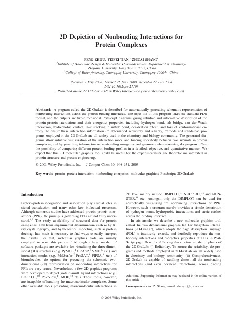
2D Depiction of Nonbonding Interactions forProtein ComplexesPENG ZHOU,1FEIFEI TIAN,2ZHICAI SHANG11Institute of Molecular Design&Molecular Thermodynamics,Department of Chemistry,Zhejiang University,Hangzhou310027,China2College of Bioengineering,Chongqing University,Chongqing400044,ChinaReceived7May2008;Revised25June2008;Accepted22July2008DOI10.1002/jcc.21109Published online22October2008in Wiley InterScience().Abstract:A program called the2D-GraLab is described for automatically generating schematic representation of nonbonding interactions across the protein binding interfaces.The inputfile of this program takes the standard PDB format,and the outputs are two-dimensional PostScript diagrams giving intuitive and informative description of the protein–protein interactions and their energetics properties,including hydrogen bond,salt bridge,van der Waals interaction,hydrophobic contact,p–p stacking,disulfide bond,desolvation effect,and loss of conformational en-tropy.To ensure these interaction information are determined accurately and reliably,methods and standalone pro-grams employed in the2D-GraLab are all widely used in the chemistry and biology community.The generated dia-grams allow intuitive visualization of the interaction mode and binding specificity between two subunits in protein complexes,and by providing information on nonbonding energetics and geometric characteristics,the program offers the possibility of comparing different protein binding profiles in a detailed,objective,and quantitative manner.We expect that this2D molecular graphics tool could be useful for the experimentalists and theoreticians interested in protein structure and protein engineering.q2008Wiley Periodicals,Inc.J Comput Chem30:940–951,2009Key words:protein–protein interaction;nonbonding energetics;molecular graphics;PostScript;2D-GraLabIntroductionProtein–protein recognition and association play crucial roles in signal transduction and many other key biological processes. Although numerous studies have addressed protein–protein inter-actions(PPIs),the principles governing PPIs are not fully under-stood.1,2The ready availability of structural data for protein complexes,both from experimental determination,such as by X-ray crystallography,and by theoretical modeling,such as protein docking,has made it necessary tofind ways to easily interpret the results.For that,molecular graphics tools are usually employed to serve this purpose.3Although a large number of software packages are available for visualizing the three-dimen-sional(3D)structures(e.g.PyMOL,4GRASP,5VMD,6etc.)and interaction modes(e.g.MolSurfer,7ProSAT,8PIPSA,9etc.)of biomolecules,the options for producing the schematic two-dimensional(2D)representation of nonbonding interactions for PPIs are very scarce.Nevertheless,a few2D graphics programs were developed to depict protein-small ligand interactions(e.g., LIGPLOT,10PoseView,11MOE,12etc.).These tools,however, are incapable of handling the macromolecular complexes.Some other available tools presenting macromolecular interactions in 2D level mainly include DIMPLOT,10NUCPLOT,13and MON-STER,14etc.Amongst,only the DIMPLOT can be used for aesthetically visualizing the nonbinding interactions of PPIs. However,such a program merely provides a simple description of hydrogen bonds,hydrophobic interactions,and steric clashes across the binding interfaces.In this article,we describe a new molecular graphics tool, called the two-dimensional graphics lab for biosystem interac-tions(2D-GraLab),which adopts the page description language (PDL)to intuitively,exactly,and detailedly reproduce the non-bonding interactions and energetics properties of PPIs in Post-Script page.Here,the following three points are the emphasis of the2D-GraLab:(i)Reliability.To ensure the reliability,the pro-grams and methods employed in2D-GraLab are all widely used in chemistry and biology community;(ii)Comprehensiveness. 2D-GraLab is capable of handling almost all the nonbonding interactions(and even covalent interactions)across binding Additional Supporting Information may be found in the online version of this article.Correspondence to:Z.Shang;e-mail:shangzc@interface of protein complexes,such as hydrogen bond,salt bridge,van der Waals(vdW)interaction,hydrophobic contact, p–p stacking,disulfide bond,desolvation effect,and loss of con-formational entropy.The outputted diagrams are diversiform, including individual schematic diagram and summarized sche-matic diagram;(iii)Artistry.We elaborately scheme the layout, color match,and page style for different diagrams,with the goal of producing aesthetically pleasing2D images of PPIs.In addi-tion,2D-GraLab provides a graphical user interface(GUI), which allows users to interact with this program and displays the spatial structure and interfacial feature of protein complexes (see .Fig.S1).Identifying Protein Binding InterfacesAn essential step in understanding the molecular basis of PPIs is the accurate identification of interprotein contacts,and based upon that,subsequent works are performed for analysis and lay-out of nonbonding mon methods identifyingprotein–protein binding interfaces include a Voronoi polyhedra-based approach,changes in solvent accessible surface area(D SASA),and various radial cutoffs(e.g.,closest atom,C b,andcentroid,etc.).152D-GraLab allows for the identification of pro-tein–protein binding interfaces at residue and atom levels.Identifying Binding Interfaces at Residue LevelAll the identifying interface methods at residue level belong toradial cutoff approach.In the radial cutoff approach,referencepoint is defined in advance for each residue,and the residues areconsidered in contact if their reference points fell within thedefined cutoff ually,the C a,C b,or centroid are usedas reference point.16–18In2D-GraLab,cutoff distance is moreflexible:cutoff distance5r A1r B1d,where r A and r B are residue radii and d is set by users(as the default d54A˚,which was suggested by Cootes et al.19).Identifying Binding Interfaces at Atom LevelAt atom level,binding interfaces are identified using closestatom-based radial cutoff approach20and D SASA-basedapproach.21For the closest atom-based radial cutoff approach,ifthe distance between any two atoms of two residues from differ-ent chains is less than a cutoff value,the residues are consideredin contact;In the D SASA-based approach,the SASA is calcu-lated twice to identify residues involved in a binding interface,once for the monomers and once for the complex,if there is achange in the SASA(D SASA)of a residue when going from themonomers to the dimer form,then it is considered involved inthe binding interface.In2D-GraLab,three manners are provided for visualizing thebinding interfaces,including spatial structure exhibition,residuedistance plot,and residue-pair contact map(see .Figs.S2–S4).Analysis and2D Layout of NonbondingInteractionsThe inputfile of2D-GraLab is standard PDB format,and the outputs are two-dimensional PostScriptfile giving intuitive and informative representation of the PPIs and their strengths, including hydrogen bond,salt bridge,vdW interaction,desolva-tion effect,ion-pair,side-chain conformational entropy(SCE), etc.The outputs are in two forms as individual schematic dia-gram and summarized schematic diagram.The individual sche-matic diagram is a detailed depiction of each nonbonding profile,whereas the summarized schematic diagram covers all nonbonding interactions and disulfide bonds across the binding interface.To produce the aesthetically high quality layouts,which pos-sess reliable and accurate parameters,several widely used pro-grams listed in Table1are employed in2D-GraLab to perform the core calculations and analysis of different nonbonding inter-actions.2D-GraLab carries out prechecking procedure for pro-tein structures and warns the structural errors,but not providing revision and refinement functions.Therefore,prior to2D-GraLab analysis,protein structures are strongly suggested to be prepro-cessed by programs such as PROCHECK(structure valida-tion),27Scwrl3(side-chain repair),28and X-PLOR(structure refinement).29Individual Schematic DiagramHydrogen BondThe program we use for analyzing hydrogen bonds across bind-ing interfaces is HBplus,23which calculates all possible posi-tions for hydrogen atoms attached to donor atoms which satisfy specified geometrical criteria with acceptor atoms in the vicinity. In2D-GraLab,users can freely select desired hydrogen bonds involving N,O,and/or S atoms.Besides,the water-mediated hydrogen bond is also given consideration.Bond strength of conventional hydrogen bonds(except those of water-mediated Table1.Standalone Programs Employed in2D-GraLab.Program FunctionReduce v3.0322Adding hydrogen atoms for proteinsHBplus v3.1523Identifying hydrogen bonds and calculatingtheir geometric parametersProbe v2.1224Identifying steric contacts and clashes at atomlevelMSMS v2.6125Calculating SASA values of protein atoms andresiduesDelphi v4.026Calculating Coulombic energy and reactionfield energy,determining electrostatic energyof ion-pairsDIMPLOT v4.110Providing application programming interface,users can directly set and executeDIMPLOT in the2D-GraLab GUI9412D Depiction of Nonbonding Interactions for Protein ComplexesFigure1.(a)Schematic representation of a conventional hydrogen bond and a water-mediated hydro-gen bond across the binding interface of IGFBP/IGF complex(PDB entry:2dsr).This diagram was produced using2D-Gralab.The conventional hydrogen bond is formed between the atom N(at the backbone of residue Leu69in chain B)and the atom OE1(at the side-chain of residue Glu3in chain I);The water-mediated hydrogen bond is formed between the atom ND1(at the side-chain of residue His5in chain B)and the atom O(at the backbone of residue Asp20in chain I),and because hydrogen positions of water are almost never known in the PDBfile,the water molecule,when serving as hydrogen bond donor,is not yet determined for its H...A length and D—H...A angle,denoted as mark ‘‘????.’’In this diagram,chains,residues,and atoms are labeled according to the PDB format.(b)Spa-tial conformation of the conventional hydrogen bond.(c)Spatial conformation of the water-mediated hydrogen bond.hydrogen bonds)is calculated using Lennard-Jones 8-6potential with angle weighting.30D U HB¼E m 3d m 8À4d m6"#cos 4h ðh >90 Þ(1)where d is the separation between the heavy acceptor atom andthe donor hydrogen atom in angstroms;E m ,the optimum hydro-gen-bond energy for the particular hydrogen-bonding atoms con-sidered;d m ,the optimum hydrogen-bond length for the particu-lar hydrogen-bonding atoms considered.E m and d m vary accord-ing to the chemical type of the hydrogen-bonding atoms.The hydrogen bond potential is set to zero when angle h 908.31Hydrogen bond parameters are taken from CHARMM force field (for N and O atoms)and Autodock (for S atom).32,33Figure 1a is the schematic representation of a conventional hydrogen bond and a water-mediated hydrogen bond across the binding interface of insulin-like growth factor-binding protein (IGFBP)/insulin-like growth factor (IGF)complex.In this dia-gram,abundant information about the hydrogen bond geometry and energetics properties is presented in a readily acceptant manner.Figures 1b and 1c are spatial conformations of the cor-responding conventional hydrogen bond and water-mediated hydrogen bond.Van der Waals InteractionThe small-probe approach developed in Richardson’s laboratory enables us to detect the all atom contact profile in protein pack-ing.2D-GraLab uses program Probe 24to realize this method to identity steric contacts and clashes on the binding interfaces.Word et al.pointed out that explicit hydrogen atoms can effec-tively improve Probe’s performance.24However,considering calculations with explicit hydrogen atoms are time-consuming,and implicit hydrogen mode is also possibly used in some cases;therefore,in 2D-GraLab,both explicit and implicit hydrogen modes are provided for users.In addition,2D-GraLab uses the Reduce 22to add hydrogen atoms for proteins,and this programis also developed in Richardson’s laboratory and can be wellcompatible with Probe.According to previous definition,vdW interaction between two adjacent atoms is classified into wide contact,close contact,small overlap,and bad overlap.24Typically,vdW potential function has two terms,a repulsive term and an attractive term.In 2D-GraLab,vdW interaction is expressed as Lennard-Jones 12-6potential.34D U SI ¼E m d m d 12À2d md6"#(2)where E m is the Lennard-Jones well depth;d m is the distance at the Lennard-Jones minimum,and d is the distance between two atoms.The Lennard-Jones parameters between pairs of different atom types are obtained from the Lorentz–Berthelodt combina-tion rules.35Atomic Lennard-Jones parameters are taken from Probe and AMBER force field.24,36Figure 2a was produced using 2D-GraLab and gives a sche-matic representation of steric contacts and clashes (overlaps)between the heavy chain residue Tyr131and two light chain res-idues Ser121and Gln124of cross-reaction complex FAB (the antibody fragment of hen egg lysozyme).By this diagram,we can obtain the detail about the local vdW interactions around the residue Tyr131.In contrast,such information is inaccessible in the 3D structural figure (Fig.2b).Desolvation EffectIn 2D-GraLab,program MSMS 25is used to calculate the SASA values of interfacial residues at atom level,and four atomic radii sets are provided for calculating the SASA,including Bondi64,Chothia75,Li98,and CHARMM83.32,37–39Bondi64is based on contact distances in crystals of small molecules;Chothia75is based on contact distances in crystals of amino acids;Li98is derived from 1169high-resolution protein crystal structures;CHARMM83is the atomic radii set of CHARMM force field.Desolvation free energy of interfacial residues is calculated using empirical additive model proposed by Eisenberg andFigure 2.(a)Schematic representation of steric contacts and overlaps between the residue Tyr131in heavy chain (chain H)and the surrounding residues Ser121and Gln124in light chain (chain L)of cross-reaction complex FAB (PDB entry:1fbi).This diagram was produced using 2D-Gralab in explicit hydrogen mode.In this diagram,interface is denoted by the broken line;Wide contact,close contact,small overlap,and bad overlap are marked by blue circle,green triangle,yellow square,and pink rhombus,respectively;Moreover,vdW potential of each atom-pair is given in the histogram,with the value measured by energy scale,and the red and blue indicate favorable (D U \0)and unfav-orable (D U [0)contributions to the binding,respectively;Interaction potential 20.324kcal/mol in the center circle denotes the total vdW contribution by residue Tyr131;Chains,residues,and heavy atoms are labeled according to the PDB format,and hydrogen atoms are labeled in Reduce format.(b)Spatial conformation of chain H residue Tyr131and its local environment.Green or yellow stands forgood contacts (green for close contact and yellow for slight overlaps \0.2A˚),blue for wide contacts [0.25A˚,hot pink spikes for bad overlaps !0.4A ˚.It is revealed that Tyr131is in an intensive clash with chain L Gln124,while in slight contact with chain L Ser121,which is well consistent with the 2D schematic diagram.9432D Depiction of Nonbonding Interactions for Protein Complexes944Zhou,Tian,and Shang•Vol.30,No.6•Journal of Computational ChemistryFigure2.(Legend on page943.)Maclachlam,40and the conformation of interfacial residues is assumed to be invariant during the binding process.D G dslv¼Xic i D A i(3)where the sum is over all the atoms;c i and D A i are the atomic solvation parameter(ASP)and the changes in solvent accessible surface area(D SASA)of atom i,respectively.Juffer et al.41 found that although desolvation free energies calculated from different ASP sets are linear correlation to each other,the abso-lute values are greatly different.In view of that,2D-GraLab pro-vides four ASP sets published in different periods:Eisenberg86, Kim90,Schiffer93,and Zhou02.40,42–44As shown in Figure3,the D SASA and desolvation free energy of interfacial residues in chain A of HLA-A*0201pro-tein complex during the binding process are reproduced in a rotiform diagram form using2D-GraLab.In this diagram,the desolvation free energy contributed by chain A is28.056kcal/ mol,and moreover,the D SASA value of each interfacial residue is also presented clearly.Ion-PairThere are six types of residue-pairs in the ion-pairs:Lys-Asp, Lys-Glu,Arg-Asp,Arg-Glu,His-Asp,and ually,ion-pairs include three kinds:salt bridge,NÀÀO bridge,and longer-range ion-pair,and found that most of the salt bridges are stabi-lizing toward proteins;the majority of NÀÀO bridges are stabi-lizing;the majority of the longer-range ion-pairs are destabiliz-ing toward the proteins.45The salt bridge can be further distin-guished as hydrogen-bonded salt bridge(HB-salt bridge)and nonhydrogen-bonded salt bridge(NHB-salt bridge or salt bridge).46In2D-GraLab,the longer-range ion-pair is neglected, and for short-range ion-pair,four kinds are defined:HB-salt bridge,NHB-salt bridge or salt bridge,hydrogen-bonded NÀÀO bridge(HB-NÀÀO bridge),and nonhydrogen-bonded N-O bridge (NHB-NÀÀO bridge or NÀÀO bridge).Although both the N-terminal and C-terminal residues of a given protein are also charged,the large degree offlexibility usually experienced by the ends of a chain and the poor structural resolution resulting from it.47Therefore,we preclude these terminal residues in the 2D-GraLab.A modified Hendsch–Tidor’s method is used for calculating association energy of ion-pairs across binding interfaces.48D G assoc¼D G dslvþD G brd(4)where D G dslv represents the sum of the unfavorable desolvation penalties incurred by the individual ion-pairing residues due to the change in their environment from a high dielectric solvent (water)in the unassociated state;D G brd represents the favorable bridge energy due to the electrostatic interaction of the side-chain charged groups.We usedfinite difference solutions to the linearized Poisson–Boltzmann equations in Delphi26to calculate the D G dslv and D G brd.Centroid of the ion-pair system is used as grid center,with temperature of298.15K(in this way,1kT50.593kcal/mol),and the Debye-Huckel boundary conditions are applied.49Considering atomic parameter sets have a great influ-ence on the continuum electrostatic calculations of ion-pair asso-ciation energy,502D-GraLab provides three classical atomic parameter sets for users,including PARSE,AMBER,and CHARMM.51–53Figure4is the schematic representation of four ion-pairs formed across the binding interface of penicillin acylase enzyme complex.This diagram clearly illustrates the information about the geometries and energetics properties of ion-pairs,such as bond length,centroid distance,association energy,and angle. The ion-pair angle is defined as the angle between two unit vec-tors,and each unit vector joins a C a atom and a side-chain charged group centroid in an ion-pairing residue.54In this dia-gram,the four ion-pairs,two HB-salt bridges,and two HB-NÀÀO bridges formed across the binding interface are given out. Association energies of the HB-salt bridges are both\21.5 kcal/mol,whereas that of the HB-NÀÀO bridges are all[20.5 kcal/mol.Therefore,it is believed that HB-salt bridge is more stable than HB-NÀÀO bridge,which is well consistent with the conclusion of Kumar and Nussinov.45,46Side-Chain Conformational EntropyIn general,SCE can be divided into the vibrational and the con-formational.55Comparison of several sets of results using differ-ent techniques shows that during protein folding process,the mean conformational free energy change(T D S)is1kcal/mol per side-chain or0.5kcal/mol per bond.Changes in vibrational entropy appear to be negligible compared with the entropy change resulted from the loss of accessible rotamers.56SCE(S) can be calculated quite simply using Boltzmann’s formulation.57S¼ÀRXip i ln p i(5)where R is the universal gas constant;The sum is taken over all conformational states of the system and p i is the probability of being in state i.Typical methods used for SCE calculations, include self-consistent meanfield theory,58molecular dynam-ics,59Monte Carlo simulation,60etc.,that are all time-consum-ing,thus not suitable for2D-GraLab.For that,the case is sim-plified,when we calculate the SCE of an interfacial residue,its local surrounding isfixed(adopting crystal conformation).In this way,SCE of each interfacial residue is calculated in turn.For the20coded amino acids,Gly,Ala,Pro,and Cys in disulfide bonds are excluded.57For other cases,each residue’s side-chain conformation is modeled as a rotamer withfinite number of discrete states.61The penultimate rotamer library used was developed by Lovell et al.,62as recommended by Dun-brack for the study of SCE.63For an interfacial residue,the potential E i of each rotamer i is calculated in both binding state and unbinding state,and subsequently,rotamer’s probability dis-tribution(p)of this residue is resulted by Boltzmann’s distribu-tion law,then the SCE in different states are solved out using eq.(5).The situation of rotamer i is defined as serious clash or nonclash:serious clash is the clash score of rotamer i more than a given threshold value,and then E i511;whereas for the9452D Depiction of Nonbonding Interactions for Protein Complexes946Zhou,Tian,and Shang•Vol.30,No.6•Journal of Computational ChemistryFigure3.Schematic representation of desolvation effect for interfacial residues in chain A of HLA-A*0201complex(PDB entry:1duz).This diagram was produced using2D-GraLab.In this diagram,the pie chart is equally divided,with each section indicates an interfacial residue in chain A;In a sec-tor,red1blue is the SASA of corresponding residue in unbinding state,the blue is in binding state,and the red is thus of D SASA;The green polygonal line is made by linking desolvation free energy ofeach interfacial residue,and at the purple circle,desolvation free energy is0(D U50),beyond thiscircle indicates unfavorable contributions to binding(D U[0),otherwise is favorable(D U\0);Inthe periphery,residue symbols are colored in red,blue,and black in terms of favorable,unfavorable,and neutral contributions to the binding,respectively;The SASA and desolvation free energy for eachinterfacial residue can be measured qualitatively by the horizontally black and green scales.[Colorfigure can be viewed in the online issue,which is available at .]Figure4.Four ion-pairs formed across the binding interface of penicillin acylase enzyme complex (PDB entry:1gkf).In thisfigure,left is2D schematic diagram produced using2D-GraLab,and posi-tively and negatively charged residues are colored in blue and red,respectively;Bridge-bonds formed between the charged atoms of ion-pairs are colored in green,blue,and yellow dashed lines for the hydrogen-bonded bridge,nonhydrogen-bonded bridge,and long-range interactions,respectively;The three parameters in bracket are ion-pair type,angle,and association energy.The right in thisfigure is the spatial conformations of corresponding ion-pairs.[Colorfigure can be viewed in the online issue, which is available at .]Figure5.(a)Loss of side-chain conformational entropy of chain B interfacial residues in HIV-1 reverse transcriptase complex(PDB entry:1rt1).This diagram was produced using2D-GraLab.In this diagram,the pie chart is equally divided,with each section indicates an interfacial residue in chain B; In a sector,side-chain conformational entropies in unbinding and binding state are colored in yellow and blue,respectively;The green polygonal line is made by linking conformational free energy of each interfacial residue;The conformational entropy and conformational free energy for each interfa-cial residue can be measured qualitatively by the horizontally black and green scales,respectively;In the periphery,residue symbols are colored in yellow,blue,and black in terms of favorable,unfavora-ble,and neutral contributions to binding,respectively.(b)The rotamers of chain B interfacial residues Lys20,Lys22,Tyr56,Asn136,Ile393,and Trp401in HIV-1reverse transcriptase complex.These rotamers were generated using2D-GraLab.[Colorfigure can be viewed in the online issue,which is available at .]9472D Depiction of Nonbonding Interactions for Protein Complexes948Zhou,Tian,and Shang•Vol.30,No.6•Journal of Computational ChemistryFigure5.(Legend on page947.)Figure6.The summarized schematic diagram of nonbonding interactions and disulfide bond across the interface of AIV hemagglutinin H5complex(PDB entry:1jsm).Length of chain A and chain B are321and160,represented as two bold horizontal lines.Interface parts in the bold lines are colored in orange,and residue-pairs in interactions are linearly linked;Conventional hydrogen bond,water-mediated hydrogen bond,ionpair,hydrophobic force,steric clash,p–p stacking,and disulfide bond are colored in aqua,bottle green,red,blue,purple,yellow,and brown,respectively;In the‘‘dumbbell shape’’symbols,residue-pair types and distances are also presented.[Colorfigure can be viewed in the online issue,which is available at .]9492D Depiction of Nonbonding Interactions for Protein Complexescase of nonclash,four potential functions are used in2D-Gra-Lab:(i)E i5E0,a constant61;(ii)statistical potential,the poten-tial energy E i of rotamer i is calculated from database-derived probability61;(iii)coarse-grained model,E i of rotamer i is esti-mated by atomic contact energies(ACE)64;and(iv)Lennard-Jones potential.58Loss of binding entropy of chain B interfacial residues in HIV-1reverse transcriptase complex is schematically repre-sented in Figure5a.Similar to desolvation effect diagram,loss of binding entropy is also presented in a rotiform diagram form. This diagram reveals that during the process of forming HIV-1 reverse transcriptase complex,the total loss of conformational free energy of chain B is9.14kcal/mol,indicating a strongly unfavorable contribution to binding(D G[0),and the average loss of conformational free energy for each residue is about0.3 kcal/mol,much less than those in protein folding(about1kcal/ mol56).Figure5b shows the rotamers of six interfacial residues in chain B.Summarized Schematic DiagramFigure6illustrates nonbonding interactions and disulfide bond formed across the binding interface of avian influenza virus (AIV)hemagglutinin H5.This protein is a dimer linked by a disulfide bond.In this diagram,conventional hydrogen bond, water-mediated hydrogen bond,ion-pair,hydrophobic force, steric clash,p–p stacking,and disulfide bond are represented in different colors.Hydrogen bonds,colored in aqua,are calculated by program HBplus.23Data in this diagram are the separation between the acceptor atom and the heavy donor atom.Water-mediated hydrogen bonds are colored in bottle green, also calculated by HBplus.23Ion-pairs,colored in red,include salt bridge and NÀÀO bridge,determined by the Kumar’s rule.45,46Data in this dia-gram are centroid distance of ion-pair.Hydrophobic forces are colored in blue.According to the D SASA rule,if the two apolar and/or aromatic interfacial resi-dues(Leu,Ala,Val,Ile,Met,Cys,Pro,Tyr,Phe,and Trp)are within the distance d\r A1r B12.8(r A and r B are side-chain radii,2.8is the diameter of water molecule),they are considered in hydrophobic contact.Data in this diagram are centroid–cent-roid separation between the two residues.Steric clashes are colored in purple.Here,only bad overlaps calculated by Probe24are presented.In2D-GraLab,explicit and implicit hydrogen modes are provided,hydrogen atoms in explicit hydrogern mode are added using Reduce.22Data in this diagram are the centroid–centroid separation when the two atoms are badly overlapped.p–p stacking are colored in yellow.Presently,studies on pro-tein stacking interactions are in lack.In2D-GraLab,p–p stack-ing is identified using the McGaughey’s rule,65i.e.,if the cent-roid–centroid separation between two aromatic rings is within 7.5A˚,they are regarded as p–p stacking(aromatic residues are Phe,Tyr,Trp,and His).This rule has been successfully adopted to study the p–p stacking across protein interfaces by Cho et al.66Besides,2D-GraLab also sets the constraints of stacking angle(dihedral angel between the planes of two aromatic rings).Data in this diagram are centroid–centroid separations between two aromatic rings in stacking state.Disulfide bonds are colored in brown,taken from the PDB records.Data in this diagram are the separations of two sulfide atoms.ConclusionsMost,if not all,biological processes are regulated through asso-ciation and dissociation of protein molecules and essentially controlled by nonbonding energetics.67Graphically-intuitive vis-ualization of these nonbonding interactions is an important approach for understanding the mechanism of a complex formed between two proteins.Although a large number of software packages are available for visualizing the3D structures,the options for producing schematic2D summaries of nonbonding interactions for a protein complex are comparatively few.In practice,the2D and3D visualization methods are complemen-tary.In this article,we have described a new2D molecular graphics tool for analyzing and visualizing PPIs from spatial structures,and the intended goal is to schematically present the nonbonding interactions stabilizing the macromolecular complex in a graphically-intuitive manner.We anticipate that renewed in-terest in automated generation of2D diagrams will significantly reduce the burden of protein structure analysis and make insights into the mechanism of PPIs.2D-GraLab is written in C11and OpenGL,and the output-ted2D schematic diagrams of nonbinding interactions are described in PostScript.Presently,2D-GraLab v1.0is available to academic users free of charge by contacting us. References1.Chothia,C.;Janin,J.Nature1974,256,705.2.Jones,S.;Thornton,J.M.Proc Natl Acad Sci USA1996,93,13.3.Luscombe,N.M.;Laskowski,R.A.;Westhead,D.R.;Milburn,D.;Jones,S.;Karmirantzoua,M.;Thornton,J.M.Acta Crystallogr D 1998,54,1132.4.DeLano,W.L.The PyMOL Molecular Graphics System;DeLanoScientific:San Carlos,CA,2002.5.Petrey,D.;Honig,B.Methods Enzymol2003,374,492.6.Humphrey,W.;Dalke,A.;Schulten,K.J Mol Graphics1996,14,33.7.Gabdoulline,R.R.;Wade,R.C.;Walther,D.Nucleic Acids Res2003,31,3349.8.Gabdoulline,R.R.;Hoffmann,R.;Leitner,F.;Wade,R.C.Bioin-formatics2003,19,1723.9.Wade,R. C.;Gabdoulline,R.R.;De Rienzo, F.Int J QuantumChem2001,83,122.10.Wallace, A. C.;Laskowski,R. A.;Thornton,J.M.Protein Eng1995,8,127.11.Stierand,K.;Maaß,P.C.;Rarey,M.Bioinformatics2006,22,1710.12.Clark,A.M.;Labute,P.J Chem Inf Model2007,47,1933.13.Luscombe,N.M.;Laskowski,R. A.;Thorntonm J.M.NucleicAcids Res1997,25,4940.14.Salerno,W.J.;Seaver,S.M.;Armstrong,B.R.;Radhakrishnan,I.Nucleic Acids Res2004,32,W566.15.Fischer,T.B.;Holmes,J.B.;Miller,I.R.;Parsons,J.R.;Tung,L.;Hu,J.C.;Tsai,J.J Struct Biol2006,153,103.950Zhou,Tian,and Shang•Vol.30,No.6•Journal of Computational Chemistry。
Waters Protein-Pak Hi Res Q Column 分离 Low Range ss

Size and Purity Assessment of Single-Guide RNAs by Anion-Exchange Chromatography (AEX)Hua Yang,Stephan M. Koza,Ying Qing YuWaters CorporationAbstractSingle-guide RNA (sgRNA) is a critical element in the CRISPR/Cas9 Technology for gene editing, the size of which usually ranges from 100 to 150 bases. In this application note, we show that the size of several sgRNAs could be estimated by comparison to a Low Range ssRNA Ladder (50–500 bases) using an optimized anion-exchange method developed on a Waters Protein-Pak Hi Res Q Column. In addition, the purity of the sgRNA samples can be assessed using the same anion exchange method, providing an informative and non-complex method for sgRNA product consistency.BenefitsWaters Protein-Pak Hi Res Q Column separation of a Low Range ssRNA Ladder with the size ranging from ■50 to 500 basesWaters Protein-Pak Hi Res Q Column separation of ssRNAs and their impurities■Size and purity estimation of ssRNAs having a size range of 100–150 mer under the same gradient conditions ■using the AEX method on Waters Protein-Pak Hi Res Q ColumnIntroductionThe discovery of clustered regularly interspaced short palindromic repeats (CRISPR)/CRISPR associated (Cas) bacterial immunity systems and the rapid adaptation of RNA guided CRISPR/CRISPR Associated Protein 9 (Cas9) Technology to mammalian cells have had a significant impact in the field of gene editing.1–3 The Cas9 protein, a non-specific endonuclease, is directed to a specific DNA site by a guide RNA (gRNA), where it makes a double-strand break of the DNA of interest. The gRNA consists of two parts: CRISPR RNA (crRNA) and trans-activating crRNA (tracrRNA). The crRNA is usually a 17–20 nucleotide sequence complementary to the target DNA, and the tracrRNA serves as a binding scaffold for the Cas9 nuclease. While crRNAs and tracrRNAs exist as two separate RNA molecules in nature, the single-guide RNA (sgRNA), which combines both the crRNA sequence and the tracrRNA sequence into a single RNA molecule, has become a commonly used format. The length of a sgRNA is in the range of 100–150 nucleotides. It is critical to characterize the sgRNA, as it is the core of the CRISPR/Cas9 technology.Anion-exchange chromatography (AEX) separates molecules based on their differences in negative surface charges. This analytical technique can be robust, reproducible, and quantitative. It is also easy to automate, requires small amounts of sample, and allows for the isolation of fractions for further analysis. AEX has been utilized in multiple areas related to gene therapy, including adeno-associated virus empty and full capsid separation, plasmid isoform separation, and dsDNA fragment separation.4–6 Since the sgRNAs are negatively charged due to the phosphate groups on the backbone, we investigated AEX for size and purity assessment of sgRNAs.In this application note, we show that using a Waters Protein-Pak Hi Res Q strong Anion-Exchange Column on an ACQUITY UPLC H-Class Bio System, a single-stranded RNA (ssRNA) ladder ranging from 50 to 500 bases can be separated and used for estimating the size of ssRNAs in the approximate range of 100–150 bases, including the sgRNAs for CRISPR/Cas9 System. Moreover, the purity of these ssRNAs can be estimated with the same gradient conditions.ExperimentalSample DescriptionHPRT (purified and crude) is a pre-designed CRISPR/Cas9 sgRNA (Hs.Cas9.HPRT1.1AA, 100 mer). GUAC is acustomized ssRNA (150 mer), which contains repeats of GUAC sequence. HPRT sgRNA and GUAC ssRNA were purchased from Integrated DNA Technologies (IDT). Rosa26 and Scrambled #2 are both pre-designedCRISPR/Cas9 sgRNAs purchased from Synthego (100 mer). Low Range ssRNA Ladder was purchased from New England Biolabs (N0364S).Method ConditionsLC ConditionsLC system:ACQUITY UPLC H-Class BioDetection:ACQUITY UPLC TUV Detector with 5 mm titaniumflow cellWavelength:260 nmVials:Polypropylene 12 x 32 mm Screw Neck Vial, withCap and Pre-slit PTFE/Silicone Septum, 300 µLVolume, 100/pk (P/N 186002639)Column(s):Protein-Pak Hi Res Q Column, 5 µm, 4.6 x 100 mm(P/N 186004931)Column temp.:60 °CSample temp.:10 °CInjection volume:1–10 µLFlow rate:0.4 mL/minMobile phase A:100 mM Tris-HClMobile phase B:100 mM Tris baseMobile phase C: 3 M Tetramethylammonium chloride (TMAC)Mobile phase D:WaterBuffer conc. to deliver:20 mMGradient Table (an AutoBlend Plus Method, Henderson-Hasselbalch derived).In the above gradient table, the buffer is 20 mM Tris pH 9.0. The initial salt concentration is set to 0 mM to ensure all the analytes are strongly bound onto the column. After 5 mins, the salt concentration is increased to 1400 mM where most of the impurities will elute, based on prior investigation. After 4 mins equilibration, the separation gradient starts. The salt concentration increases linearly from 1400 m to 2100 mM in 20 mins for the Low Range ssRNA Ladder separation, as well as individual ssRNAs. Then it is ramped up to 2400 mM to strip off any remaining bound molecules. Finally, an equilibration step to the initial condition takes place, preparing for the next injection.An equivalent gradient table for a generic quaternary LC system is shown above.Data ManagementChromatography software:Empower 3 (FR 4)Results and DiscussionSize AssessmentVarious mobile phase conditions were tested using a Low Range ssRNA Ladder for size assessment of the ssRNAs, including pH (7.4 and 9.0), column temperature (30 °C and 60 °C) and salt (NaCl and TMAC).The results from the optimal conditions are shown in Figure 1B. Using a pH 9.0 Tris buffer with 60 °C column temperature and a TMAC salt gradient, the Low Range ssRNA Ladder (50–500 bases) along with four pre-made sgRNAs (100 mer), and one customized ssRNA (150 mer) were separated on a Waters Protein-Pak Hi Res Q Column. The separation for the Low Range ssRNA Ladder on this strong anion exchange column was very similar to that on an agarose gel, as shown in Figure 1A. A calibration curve was constructed based on the retention time and the logarithm of the number of bases of each ssRNA in the ladder (Figure 1C, blue dots). Thelinear fit from the Low Range ssRNA Ladder indicates a strong correlation between the logarithm of the size andthe retention time (R2=0.993). Using this plot, the size of the ssRNAs was calculated from their individual retention time. The percent error is calculated using the formula {(calculated size – theoretical size)/theoretical size}. The percent error was less than 6% for all the RNAs tested (Figure 1d), as evidenced by the orange data points residing on or very closely to the trendline of the calibration curve. Notice that small percent error was obtained from four pre-made sgRNAs from two different manufacturers and a customized ssRNA with an artificial sequence. Although ssRNAs with shorter than 100 bases and larger than 150 bases were not tested, it is possible that this method can be used for the ssRNAs size assessment in the range of 50–500 bases.Figure 1A.Agarose gel separation of Low Range ssRNA Ladder (Reprinted from (2021) with permission from New England Biolabs); 1B. Anion-exchange separation of Low Range ssRNA Ladder and ssRNAs on a Waters Protein-Pak Hi Res Q Column; 1C. A plot of log(size) vs. retention time of Low Range ssRNA Ladder (blue dots) and individual ssRNAs (orange dots); 1D. Size estimation of individual ssRNAs based on retention time and calibration curve. Small percent error was obtained for all ssRNAs.It is noteworthy that a mobile phase condition with pH 7.4 Tris buffer, 60 °C column temperature and a TMAC salt gradient also resulted in good size estimation with percent error <5% for all pre-made sgRNAs (100 mer) and ~12% for the artificially made GUAC ssRNA (150 mer). Overall, 60 °C column temperature resulted in one singlepeak for each ssRNA which is needed to determine the retention time of the peak for size assessment. 30 °C column temperature resulted in more than one major peaks, which are presumably the isomers of the ssRNAs. Multiple peaks were also observed when using NaCl as the salt, regardless of the pH and column temperature.Purity AssessmentPurified and crude HPRT sgRNA was separated on the Protein-Pak Hi Res Q Column (Figure 2) using the same gradient conditions for size assessment. The relative purities of the crude and purified samples were measured as 37.4% and 88.0%, respectively, based on the peak areas indicated. The majority of the impurities eluted prior to 50 bases although lower abundance impurities appear to be present up to the size of the HPRT sgRNA.Figure 2. Crude and purified HPRT sgRNA for CRISPR/Cas 9 System were separated on a Waters Protein-Pak Hi Res Q Column using the same conditions as in Figure 1B (see Experimental for details).ConclusionAnion-exchange chromatography is robust, reproducible, easy to automate, yields quantitative information, andrequires a small amount of sample. We demonstrate here that the components of a Low Range ssRNA Ladder, ranging from 50 to 500 bases, can be separated on a Waters Protein-Pak Hi Res Q Column with a linear correlation between the log of base-number and observed retention time when TMAC is used as an elution salt. The size of ssRNAs ranging from 100 to 150 bases can be estimated by comparing the retention time of the ssRNAs with that of the Low Range ssRNA Ladder. In addition, the purity of a sgRNAs may also be observed from the same chromatographic separation. This method can potentially be applied to the analysis of sgRNAs which are the key element for CRISPR/Cas9 gene editing technology.ReferencesDunbar C E, High K A, J. Joung K, Kohn D B, Ozawa K, Sadelain M. Gene Therapy Comes of Age. Science 1.2018; 359: 175.2.Rath D, Amlinger L, Rath A, Lundgren M. The CRISPR-Cas Immune System: Biology, Mechanisms and Applications. Biochimie 2015; 117: 119–128.3.Patrick D. Hsu P D, Eric S. Lander E S, and Zhang F. Development and Applications of CRISPR-Cas9 for Genome Engineering. Cell 2014; 157: 1262–1278.Yang H, Koza S and Chen W. Anion-Exchange Chromatography for Determining Empty and Full Capsid4.5.Yang H, Koza S and Chen W. Plasmid Isoform Separation and Quantification by Anion-Exchange6.Yang H, Koza S and Chen W. Separation and Size Assessment of dsDNA Fragments by Anion-ExchangeFeatured Products■■720007428, November 2021© 2021 Waters Corporation. All Rights Reserved.。
陈支越乳酸阈强度的4种训练方式对水球运动员有氧耐力的

第27卷 成都体育学院学报 2001年2001年第4期 Journal of Chengdu Physical Education Institute No .4.2001 第一作者简介:陈支越(1964—),女,河北人,讲师,研究方向:教学与训练。
收稿日期:2000—12—15乳酸阈强度的4种训练方式对水球运动员有氧耐力的影响陈支越1,杨尚春2,李建萍3(1.广西民族学院体育系,南宁530006;2.广西右江民族师专,百色533000;3.广西银行学校,南宁530007) 摘要:运用个体乳酸阈(ILA T )对30名青少年水球运动员有氧耐力的训练和评价进行实验研究,纵向观察ILA T 强度的匀速游、间歇游、变速游和混合游4种训练方式对有氧耐力的影响。
结果表明:4种不同方式的训练,对水球运动员I LA T 时的游速和心率及其他心肺功能指标产生不同的影响,从有氧耐力的良好生理和训练效应来看,混合游最优,变速游和间歇游次之,匀速游最差。
关键词:水球;运动员;个体乳酸阈;训练方式;有氧耐力 中图分类号:G 804.7 文献标识码:A 文章编号:1001—9154(2001)04—0082—03 水球运动是在间歇性、高强度的反复冲刺游以及激烈的拼抢中进行的混合性运动项目。
一场4节28min 激烈的水球比赛,运动员的游动距离可达2500m 以上。
提高运动员的体能水平是现代水球训练的一项重要内容。
体力差是国内各级运动队,尤其是青少年运动员普遍存在的问题,主要表现在第3、4节比赛时耐力明显不足,完成动作速度明显放慢,技术难以发挥,对抗能力减弱,造成全队整体水平下降[1]。
应该用个体乳酸阈(乳酸无氧阈)指标来确定运动员个体训练强度,进行耐力训练和评价运动员有氧耐力水平。
本研究的目的是:运用个体乳酸阈对青少年水球运动员的有氧耐力训练进行评价,纵向观察乳酸阈强度的4种训练方法对提高运动员的有氧训练的生理效应,为在水球运动训练实践中运用个体乳酸阈指标和选择能使有氧耐力训练获得良好效应的训练方式提供参考。
Sensitive Immunoluminometric Assay for the Detection of Procalcitonin

to be no substantive objection to implementing the sug-gestion by Favus(11)with45Ca as the tracer. However,whether a stable or a radioactive tracer is used,there is now a suitable algorithm for both men and women,requiring only a single serum sample and pro-viding results within1day.This study was supported in part by an agreement with the University of Pittsburgh,Graduate School of Public Health,by contracts with Roots,Inc.and DepoMed,Inc., by a grant from Health Future Foundation,and by Creighton University funds.References1.Nordin BEC,Need AG,Morris HA,Horowitz M,Chatterton BE,Sedgwick AW.Bad habits and bad bones.In:Burckhardt P,Heaney RP,eds.Nutritional aspects of osteoporosis’94(Proceedings of2nd International Symposium on Osteoporosis,Lausanne,May1994).Rome:Ares-Serono Symposia, 1995:1–25.2.deGrazia JA,Ivanovich P,Fellows H,Rich C.A double isotope method formeasurement of intestinal absorption of calcium in man.J Lab Clin Med 1965;66:822–9.3.Heaney RP,Recker RR.Estimation of true calcium absorption.Ann InternMed1985;103:516–21.4.Heaney RP,Recker RR.Estimating true fractional calcium absorption.AnnIntern Med1988;108:905–6.5.Ensrud KE,Duong T,Cauley JA,Heaney RP,Wolf RL,Harris E,et al.Lowfractional calcium absorption increases the risk of hip fracture in women with low calcium intake.Ann Intern Med2000;132:345–53.6.Jackson JD,Dunlevy JA.The orthogonal least squares slope estimator:interval estimation and hypothesis testing under the assumption of bivariate normality.American Statistical Association Proceedings of the Business and Economics Statistics Section1981;1:294–7.7.Barger-Lux MJ,Heaney RP,Recker RR.Time course of calcium absorption inhumans:evidence for a colonic component.Calcif Tissue Int1989;44:308–11.8.Geigy Pharmaceuticals.Documenta Geigy scientific tables,6th ed.Ardsley,NY:Geigy Pharmaceuticals,1962:538.9.Heaney RP.Evaluation and interpretation of calcium kinetic data in man.ClinOrthop1963;31:153–83.10.Heaney RP,Weaver CM,Barger-Lux J.Food factors influencing calciumavailability.In:Burckhardt P,Heaney RP,eds.Nutritional aspects of osteoporosis’94(Proceedings of2nd International Symposium on Osteo-porosis,Lausanne,May1994).Rome:Ares-Serono Symposia,1995:229–41.11.Favus M.Intestinal calcium absorption:have we absorbed enough fromresearch to have a test for the patient?J Bone Miner Res1989;4:461–2.som S,Ibbertson K,Hannan S,Shaw D,Pybus J.Simple test of intestinalcalcium absorption measured by stable strontium.BMJ1987;295:231–4.13.Sips AJAM,van der Vijgh WJF,Barto R,Netelenbos JC.Intestinal strontiumabsorption:from bioavailability to validation of a simple test representative for intestinal calcium absorption.Clin Chem1995;41:1446–50.14.Wasserman RH.Strontium as a tracer for calcium in biological and clinicalresearch.Clin Chem1998;44:437–9.15.Heaney RP.Absorbing calcium.Clin Chem1999;45:161–2.Sensitive Immunoluminometric Assay for the Detection of Procalcitonin,Nils G.Morgenthaler,*Joachim Struck, Christina Fischer-Schulz,and Andreas Bergmann(Research Department,B⅐R⅐A⅐H⅐M⅐S AG,Biotechnology Centre, D-16761Hennigsdorf/Berlin,Germany;*author for cor-respondence:fax49-3302-883-451,e-mail n.morgenthaler@ brahms.de)Procalcitonin(PCT)and other calcitonin precursors are detectable in various conditions leading to systemic in-flammatory response syndrome.Among them are pancre-atitis(1,2),burns(3),polytrauma(4),and most impor-tantly,bacterial infection(5).PCT reflects the severity of bacterial infection and has been used as a marker for the diagnosis and therapeutic monitoring of sepsis,severe sepsis,and septic shock of bacterial origin(6–10).The usual two-sided chemiluminescence assay[immunolumi-nometric assay(ILMA)]for PCT has a functional assay sensitivity(FAS)of300ng/L.This FAS is sufficient for the monitoring of septic patients in intensive care units,but the usefulness of the present ILMA in the usual hospital or outpatient setting is limited.Furthermore,except for an initial report on PCT and other calcitonin precursors in a few controls(8),it has not been possible to define the range of PCT in healthy individuals or to determine whether increased PCT exerts a pathophysiologic role (11–13).We developed a new PCT assay with aϾ30-fold lower FAS compared with the established ILMA and measured PCT values in500healthy controls.Samples were obtained from healthy blood donors(age range,18–62years;241males,259females)with no history of acute or chronic disease and with no symptoms of the common cold for the last7days.Written consent was obtained from all donors.For the PCT assay,tubes were coated with a monoclo-nal antibody specific for the katacalcin part of PCT.This antibody binds to amino acids102–111of PCT(ERDHR-PHVSM).Coating of the antibody was done for20h on polystyrene tubes(2.0g/tube)in0.3mL of buffer(10 mmol/L Tris-HCl,pH7.8,10mmol/L NaCl).Tubes were blocked with10mmol/L sodium phosphate buffer con-taining30q/L Karion FP,5g/L protease-free bovine serum albumin(Sigma),pH6.8,and lyophilized.A poly-clonal sheep antibody specific for the calcitonin part of PCT was used as tracer.This antibody was raised to peptide69–79(GTYTQDLNKFH)of PCT and was affini-ty-purified on a calcitonin-sulfolink column and subse-quently labeled with acridinium ester as follows:100g of antibody in20mmol/L sodium phosphate buffer,pH 8.0,was incubated for20min at room temperature with10l of acridinium ester(1g/L in acetonitrile;Hoechst AG). Labeled antibody was purified by HPLC using a Knauer hydroxyapatite column(buffer gradient,1–500mmol/L potassium phosphate,pH6.8;flow rate,0.8mL/min). PCT was measured in a coated-tube assay in which100L of a patient sample or calibrator was added in dupli-cate to each antibody-coated tube and incubated for30 min at room temperature;200L of tracer containing acridinium ester-labeled anti-PCT antibody was then added,followed by a2-h incubation at room temperature. Tubes were washed five times with2mL of standard LUMItest®washing buffer(B⅐R⅐A⅐H⅐M⅐S AG),and detec-tion was performed in a luminometer(detection time per sample,1s).This assay system was named B⅐R⅐A⅐H⅐M⅐S ProCa-S®to distinguish it from the similar LUMItest PCT®(B⅐R⅐A⅐H⅐M⅐S AG).Relative light units for the chemiluminescence assay were expressed in ng/L PCT as calculated from a calibration curve that was included in every analytical run.788Technical BriefsTo prepare calibrators,human PCT (amino acids 1–115)was overexpressed in Escherichia coli and purified by anion-exchange and reversed-phase chromatography as described previously (14).For the highest calibrator (S6),5000ng/L human recombinant PCT was added to horse serum (Sigma).This was calibrated by use of the LUMItest PCT and diluted to prepare calibrators S2to S5with final concentrations of 20,100,500,2000,and 5000ng/L.The lowest calibrator,S1(PCT-free horse serum),was defined as 5ng/L PCT to allow logarithmic plotting of the calibration curve.As controls,horse sera containing 50ng/L (control I)and 1000ng/L (control II)were added at the beginning and end of each run.The intraassay imprecision was determined by measur-ing 23human serum samples covering the range of the calibration curve in 10parallel determinations.The in-traassay CV was Ͻ8%in samples containing 8–4000ng/L PCT and Ͻ15%in samples containing Ͻ8ng/L PCT.The interassay imprecision was determined by measuring the same samples on 10different days (Fig.1A).The func-tional assay sensitivity (interassay CV Ͻ20%)was Ͻ7ng/L PCT.To compare this new assay with the established LUMI-test PCT,we measured 71serum samples from patients with sepsis who had PCT values between 250and 5000ng/L in both assays.The mean difference (SD)was 11.6(256.4)ng/L (15)(Fig.1B).In 500healthy individuals,the range was Ͻ7to 63ng/L PCT.The median was 13.5ng/L (95%confidence interval for the mean,12.6–14.7ng/L).The 97.5percentile of the population studied was 42.5ng/L (Fig.1C).There were no significant differences in the range and median PCT values between males and females or among age groups.Similar low concentrations were reported by Snider et al.(8),who used HPLC-extracted calcitonin precursors from pooled serum of healthy males.We conclude that the proposed assay can measure PCT in healthy individuals or patients without systemic in-flammatory response syndrome/sepsis.PCT values in healthy individuals are more than 10-fold lower than the clinical cutoff used for the diagnosis of severe systemic bacterial infection or sepsis (500ng/L).At present,PCT can not be used for the diagnosis or monitoring of local bacterial infections because the established ILMA does not detect PCT concentrations Ͻ300ng/L.The proposed assay may be useful to evaluate whether local bacterial infections increase PCT above the reference intervals.We thank Tao Chen,Uwe Zingler,and Elke Seidel-Mu ¨ller for excellent technical assistance.We also acknowledge Dr.Barbara Thomas for helpful discussions.References1.Rau B,Steinbach G,Gansauge F,Mayer JM,Grunert A,Beger HG.The potential role of procalcitonin and interleukin 8in the prediction of infected necrosis in acute pancreatitis .Gut 1997;41:832–40.2.Brunkhorst FM,Eberhard OK,Brunkhorst R.Early identification ofbiliaryFig.1.Characteristics of the ProCa-S assay for PCT.(A ),interassay CVs for the same samples on 10different days.(B ),Bland –Altman plot comparing difference between the results obtained with the LUMItest and ProCa-S assays as a function of the mean values obtained with both assays (15).(C ),frequency distribution of PCT values in 500healthy controls.Clinical Chemistry 48,No.5,2002789pancreatitis with procalcitonin[Letter].Am J Gastroenterol1998;93: 1191–2.3.Nylen ES,O’Neill W,Jordan MH,Snider RH,Moore CF,Lewis M,et al.Serumprocalcitonin as an index of inhalation injury in burns.Horm Metab Res 1992;24:439–43.4.Mimoz O,Benoist JF,Edouard AR,Assicot M,Bohuon C,Samii K.Procalci-tonin and C-reactive protein during the early posttraumatic systemic inflam-matory response syndrome.Intensive Care Med1998;24:185–8.5.Assicot M,Gendrel D,Carsin H,Raymond J,Guilbaud J,Bohuon C.Highserum procalcitonin concentrations in patients with sepsis and infection.Lancet1993;341:515–8.6.Dandona P,Nix D,Wilson MF,Aljada A,Love J,Assicot M,et al.Procalcitoninincrease after endotoxin injection in normal subjects.J Clin Endocrinol Metab1994;79:1605–8.7.Gendrel D,Assicot M,Raymond J,Moulin F,Francoual C,Badoual J,et al.Procalcitonin as a marker for the early diagnosis of neonatal infection.J Pediatr1996;128:570–3.8.Snider RH Jr,Nylen ES,Becker KL.Procalcitonin and its component peptidesin systemic inflammation:immunochemical characterization.J Invest Med 1997;45:552–60.9.Whang KT,Steinwald PM,White JC,Nylen ES,Snider RH,Simon GL,et al.Serum calcitonin precursors in sepsis and systemic inflammation.J Clin Endocrinol Metab1998;83:3296–301.10.Muller B,Becker KL,Schachinger H,Rickenbacher PR,Huber PR,ZimmerliW,et al.Calcitonin precursors are reliable markers of sepsis in a medical intensive care unit.Crit Care Med2000;28:977–83.11.Nylen ES,Whang KT,Snider RH Jr,Steinwald PM,White JC,Becker KL.Mortality is increased by procalcitonin and decreased by an antiserum reactive to procalcitonin in experimental sepsis.Crit Care Med1998;26: 1001–6.12.Muller B,White JC,Nylen ES,Snider RH,Becker KL,Habener JF.Ubiquitousexpression of the calcitonin-I gene in multiple tissues in response to sepsis.J Clin Endocrinol Metab2001;86:396–404.13.Domenech VS,Nylen ES,White JC,Snider RH,Becker KL,Landmann R,etal.Calcitonin gene-related peptide expression in sepsis:postulation of microbial infection-specific response elements within the calcitonin I gene promoter.J Invest Med2001;49:514–21.14.Wrenger S,Kahne T,Bohuon C,Weglohner W,Ansorge S,Reinhold D.Amino-terminal truncation of procalcitonin,a marker for systemic bacterial infections,by dipeptidyl peptidase IV(DP IV).FEBS Lett2000;466:155–9.15.Bland JM,Altman DG.Statistical methods for assessing agreement be-tween two methods of clinical ncet1986;1:307–10. Comparison of Cardiac Troponin I in Serum and Hep-arin Plasma with the Dimension RxL Assay,Alberto Cerutti,*Leonora Corsini,Roberto Finotto,and Carlo Perazzi (Clinical Laboratory,S.Biagio Hospital,28845Domodos-sola,Italy;*author for correspondence:fax39-0324-4961247,e-mail labanalisidomo@asl14.it.)Cardiac troponin[I(cTnI)and T(cTnT)]assays in blood have rapidly become alternatives to older methods for detecting myocardial damage(1,2).Furthermore,the re-cently redefined criteria for myocardial infarction that are used to classify patients with acute coronary syndrome have been established on the basis of increased serum/plasma cTnI or cTnT(3).The National Academy of Clinical Bio-chemistry has recommended the use of plasma rather than serum as the specimen of choice(4),citing improved turn-around times and potentially avoiding incomplete serum separation that may influence some methods to produce falsely increased results(5).However,some studies have shown lower cTnI and cTnT concentrations in plasma than in serum(6,7).Because heparin effects vary among different analytical methods,we performed a study to evaluate cTnI concentrations in plasma and serum specimens assayed on the Dimension RxL(Dade Behring).We evaluated assay imprecision using lyophilized controlsera with three different concentrations of cTnI(0.57,5,and15g/L)that were analyzed10times in one analytical run for the determination of within-run imprecision and24times on24different days for the determination of between-run imprecision.Our results confirmed the manufacturer’sclaims that within-and between-run imprecisions(CVs)were2.8–3.9%and2.9–4.1%,respectively.The analyticalsensitivity was0.04g/L,defined as the concentration corresponding to a signal that was2SD above the signaldetected for the0g/L cTnI calibrator(nϭ20).To compare plasma and serum cTnI,100paired ran-domized blood samples were obtained from patients admitted to the Division of Cardiology(nϭ64)or to the Emergency Room(nϭ36)of our hospital for acute myocardial infarction(AMI)or suspected AMI.The paired samples were drawn in parallel into tubes without anticoagulant(cat.no.367615;Becton Dickinson)and into tubes with lithium heparin(ϳ65IU of heparin/mL plasma considering an hematocrit of50%;cat.no.367684; Becton Dickinson).According to the consensus document of the European and American Cardiologists(3),blood was obtained from our patients on hospital admission,at 6to9h and again at12to24h if the earlier samples were negative and the clinical index of suspicion was high.We used a cTnI cutoff for AMI at0.6g/L as indicated by the manufacturer.The Dimension RxL assay,like all the other troponin assays(8),does not comply with the new consensus requirement(3)of aՅ10%CV at the99th percentile(0.07g/L)of a reference group.Within10–15 min after venipuncture,both tubes were centrifuged at 3000g for10min,and the serum and heparin-plasma samples were frozen atϪ20°C until cTnI determination. Before assay,the specimens were thawed,gently mixed by inverting the tubes five to eight times,and recentri-fuged at3000g for10min.The cTnI concentration ranges for serum and plasmawere0.24–48.5g/L and0.28–48.2g/L,respectively, well above the detection limit of the assay(0.04g/L as indicated above).No significant difference was foundbetween serum and plasma cTnI concentrations(101.7Ϯ2.4%;t-test for paired data,Pϭ0.90),with an excellentcorrelation(rϭ0.993;PϽ0.001;cTnI plasmaϭ1.00ϫcTnI serumϪ0.02).Whereas the ratio between plasma and serum cTnI concentrations was rather wide(range,53.8–125%),no significant correlation was found between thisratio and the mean plasma-serum cTnI concentration(Pϭ0.63).Interestingly,only one sample showed a high un-derestimate in plasma cTnI concentration compared withserum(ϳ46%).This sample gave the same result whenrepeatedly analyzed(three times)to exclude sporadicerror attributable to a small clot,bubble,or misidentifica-tion.For the other99samples,the plasma/serum cTnIratio was between0.76and1.25(Fig.1).To clarify this problem,we also carried out heparintitration experiments by adding increasing volumes ofheparin(5000IU/mL)to serum aliquots of10samples(with cTnI between0.24and20.2g/L)to final concen-790Technical Briefs。
一种基于PRI变换的雷达信号分选方法

一种基于PRI变换的雷达信号分选方法王海滨;马琦【摘要】With the signal environment of information warfare increasingly complicated, the radar signal sorting technology, as one of development directions of modern radar, is of great importance to radar reconnaissance. Several radar signal deinterleav-ing methods are proposed based on PRI parameter. The traditional PRI transform can overcome the subharmonic problem pro-duced in the histogram statistic methods, but has a poor performance on anti-jitter. The paper begins with a discussion of the im-proved PRI transform which overcomes the disadvantages of traditional PRI method effectively, followed by the description of the algorithm simulation. Finally, a method for sorting pulse repetition intervals of staggered PRI is discussed.%信息作战环境日益复杂,而雷达信号分选技术是作为现代信息对抗领域的重要发展方向之一,对于雷达侦察非常重要.对于雷达信号分选,基于PRI参数提出了很多分选方法.传统的PRI变换能克服直方图统计法中的子谐波问题,但抗抖动性差.讨论了修正的PRI变换分选算法,有效地克服了传统PRI变换的缺点,并对算法进行了计算机仿真.最后还讨论了重频参差抖动脉冲序列的分选方法.【期刊名称】《现代电子技术》【年(卷),期】2013(036)001【总页数】4页(P28-31)【关键词】脉冲重复间隔;信号分选;PRI变换;重频参差【作者】王海滨;马琦【作者单位】海军航空兵学院,辽宁葫芦岛125001;南通吉尔达集团公司,江苏南京226300【正文语种】中文【中图分类】TN971-340 引言在雷达侦察系统中,信号处理的主要任务是对前端输出的实时脉冲信号描述字流进行信号分选、参数估计、辐射源识别。
Arlequin (version 3.0)

A P P L I C A T I O N N O T E Arlequin (version 3.0): An integrated software package for population genetics data analysisLaurent Excoffier, Guillaume Laval, Stefan SchneiderComputational and Molecular Population Genetics Lab, , Zoological Institute, University of Berne, Baltzerstrasse 6, 3012 Berne, SwitzerlandIntroductionMost genetic studies on non-model organisms require a description of the pattern of diversity within and be-tween populations, based on a variety of markers often including mitochondrial DNA (mtDNA) sequences and microsatellites. The genetic data are processed to extract information on the mating system, the extent of popu-lation subdivision, the past demography of the population, or on departure from selective neutrality at some loci. A series of computer packages have been developed in the last 10 years to assist researchers in performing basic population genetics analyses like Arlequin2 (Schneider et al. 2000), DNASP (Rozas et al. 2003), FSTAT (Goudet 1995), GENEPOP (Raymond and Rousset 1995b), or GENETIX (Belkhir et al. 2004). These programs have been widely used in the molecular ecology and conservation genetics community (Labate 2000; Luikart and England 1999; Schnabel et al. 1998). Among these, Arlequin is a very versatile (though not universal) pro-gram, and complements the other programs listed above. It can handle several data types like RFLPs, DNA se-quences, microsatellite data, allele frequencies, or standard multi-locus genotypes, while allowing the user to carry out the same types of analyses irrespective of the data types.We present here the version 3 of Arlequin with additional methods extending its capacities for the handling of unphased multi-locus genotypes and for the estimation of parameters of a spatial expansion. Note that these new developments are mainly implementations of new methodologies developed in our lab. We believe these methods will be useful to the research community, but we do not claim that alternative methods implemented by other groups in other programs are inadequate. A new graphical interface has been developed to provide a better integration of the different analyses into a common framework, and an easier exploration of the data by performing a wide variety of analyses with different settings. The tight coupling of Arlequin with the simula-tion programs SIMCOAL2 (Laval and Excoffier 2004) and SPLATCHE (Currat et al. 2004) should also make it useful to describe patterns of genetic diversity under complex evolutionary scenarios.Methods implemented in ArlequinArlequin provides methods to analyse patterns of genetic diversity within and between population samples.Intra-population methods• Computation of different standard genetic indices, like the number of segregating sites, the number of dif-Excoffier et alferent alleles, the heterozygosity, the basecomposition of DNA sequences, gene diver-sity, or the population effective size N e scaledby the mutation rate μ as θ=4N e u.• Maximum-likelihood estimation of allele and haplotype frequencies via the EM algorithm(Excoffier and Slatkin 1995).• Estimation of the gametic phase from multi-locus genotypes via the Excoffier-Laval-Balding (ELB) algorithm (Excoffier et al.2003).• Estimation of the parameters of a demographic (Rogers and Harpending 1992; Schneider andExcoffier 1999) or a spatial (Excoffier 2004;Ray et al. 2003) expansion, from the mismatchdistribution computed on DNA sequences.• Calculation of several measures of linkage dis-equilibrium (LD) like D, D', or r2(Hedrick1987), and test of non-random association ofalleles at different loci when the gametic phaseis known (Weir 1996) or unknown (Slatkinand Excoffier 1996).• Exact test of departure from Hardy-Weinberg equilibrium (Guo and Thompson 1992).• Computation of Tajima’s D (Tajima 1989) and Fu's F S(Fu 1997) statistics, and test of theirsignificance by coalescent simulations(Hudson 1990; Nordborg 2003) under the infi-nite-site model.• Tests of selective neutrality under the infinite-alleles model, like the Ewens-Watterson test(Slatkin 1996; Watterson 1978), and Chak-raborty’s amalgamation test (Chakraborty1990).Inter-population methods• Search for shared haplotypes between popula-tions• Analysis of population subdivision under the AMOVA framework (Excoffier 2003; Excof-fier et al. 1992), with three hierarchical levels:genes within individuals, individuals withindemes, demes within groups of demes. Com-putation of F-statistics like the local inbreed-ing coefficient F IS or the index of populationdifferentiation F ST.• Computation of genetic distances between populations related to the pairwise F ST index(Gaggiotti and Excoffier 2000; Reynolds et al.1983; Slatkin 1995).• Exact test of population differentiation (Goudet et al. 1996; Raymond and Rousset1995a).• A simple assignment test of individual geno-types to populations according to their likeli-hood (Paetkau et al. 1997).• Computation of correlations or partial correla-tions between a set of 2 or 3 distance matrices(Mantel test: Smouse et al. 1986)New features in Arlequin 3• Version 3 of Arlequin integrates the core com-putational routines and the interface in a singleprogram written in C++ for the Windows envi-ronment. The interface has been entirely redes-igned to provide better usability.• Incorporation of two new methods to estimate gametic phase and haplotype frequencies:◊ The ELB algorithm (Excoffier et al.2003) is a pseudo-Bayesian approachaiming at reconstructing the gameticphase of multi-locus genotypes, and theestimation of the haplotype frequenciesare a by-product of this process. Phaseupdates are made on the basis of a win-dow of neighbouring loci, and the win-dow size varies according to the locallevel of linkage disequilibrium.◊ The EM zipper algorithm, which is an extension of the EM algorithm for esti-mating haplotype frequencies (Excoffierand Slatkin 1995), aims at estimating thehaplotype frequencies in unphasedmulti-locus genotypes. The estimation ofthe gametic phases are a by-product ofthis process. It proceeds by adding locione at a time and progressively extend-ing the length of the reconstructed haplo-Arlequin 3.0Excoffier et alReferencesAdkins RM. 2004. Comparison of the accuracy of methods of computational haplotype inference using a large empirical dataset. BMC Genet. 5:22.Belkhir K, Borsa P, Chikhi L et al. 2004. GENETIX 4.05, logiciel sous Win-dows pour la génétique des populations. Laboratoire Génome, Popula-tions, Interactions, CNRS UMR 5000, Université de Montpellier II,Montpellier.Chakraborty R. 1990. Mitochondrial DNA polymorphism reveals hidden het-erogeneity within some Asian populations. Am J Hum Genet. 47: 87-94.Currat M, Ray N and Excoffier L. 2004. SPLATCHE: a program to simulate genetic diversity taking into account environmental heterogeneity.Mol Ecol. 4: 139-142.Excoffier L. 2003. Analysis of Population Subdivision. In Balding D Bishop M, and Cannings C, eds. Handbook of Statistical Genetics, 2nd Edi-tion. New York: John Wiley & Sons, Ltd. p 713-750.Excoffier L. 2004. Patterns of DNA sequence diversity and genetic structure after a range expansion: lessons from the infinite-island model. MolEcol. 13: 853-864.Excoffier L, Laval G and Balding D. 2003. Gametic phase estimation over large genomic regions using an adaptive window approach. Mol Ecol.1: 7-19.Excoffier L and Slatkin M. 1995. Maximum-likelihood estimation of molecular haplotype frequencies in a diploid population. Mol Biol Evol. 12: 921-927.Excoffier L, Smouse P and Quattro J. 1992. Analysis of molecular variance inferred from metric distances among DNA haplotypes: Application tohuman mitochondrial DNA restriction data. Genetics. 131: 479-491. Fu Y-X. 1997. Statistical tests of neutrality of mutations against population growth, hitchhiking and backgroud selection. Genetics. 147: 915-925. Gaggiotti O and Excoffier L. 2000. A simple method of removing the effect ofa bottleneck and unequal population sizes on pairwise genetic dis-tances. Proceedings of the Royal Society London B. 267: 81-87. Goudet J. 1995. Fstat version 1.2: a computer program to calculate F-statistics.J Heredity. 86: 485-486.Goudet J, Raymond M, de Meeüs T et al. 1996. Testing differentiation in dip-loid populations. Genetics. 144: 1933-1940.Guo S and Thompson E. 1992. Performing the exact test of Hardy-Weinberg proportion for multiple alleles. Biometrics. 48: 361-372.Hedrick P. 1987. Gametic disequilibrium measures: proceed with caution.Genetics. 117: 331-3412.Hudson RR. 1990. Gene genealogies and the coalescent process. In Futuyma DJ and Antonovics JD, eds. Oxford Surveys in Evolutionary Biology.New York: Oxford University Press. p 1-44.Labate JA. 2000. Software for Population Genetic Analyses of Molecular Marker Data. Crop Sci. 40: 1521-1528.Laval G and Excoffier L. 2004. SIMCOAL 2.0: a program to simulate genomic diversity over large recombining regions in a subdivided populationwith a complex history. Bioinformatics. 20: 2485-2487.Luikart G and England PR. 1999. Statistical analysis of microsatellite DNA data. Trends Ecol Evol. 14: 253-256.Nordborg M. 2003. Coalescent Theory. In Balding D Bishop M, and Cannings C, eds. Handbook of Statistical Genetics, 2nd edition. New York: JohnWiley & Sons Ltd. p 602-635.Paetkau D, Waits LP, Clarkson PL et al. 1997. An empirical evaluation of genetic distance statistics using microsatellite data from bear (Ursidae)populations. Genetics. 147: 1943-1957.Ray N, Currat M and Excoffier L. 2003. Intra-Deme Molecular Diversity in Spatially Expanding Populations. Mol. Biol. Evol. 20: 76-86. Raymond M and Rousset F. 1995a. An exact test for population differentiation.Evolution. 49: 1280-1283.Raymond M and Rousset F. 1995b. GENEPOP Version 1.2: Population genet-ics software for exat tests and ecumenicism. J Heredity. 248-249. Reynolds J, Weir BS and Cockerham CC. 1983. Estimation for the coancestry coefficient: basis for a short-term genetic distance. Genetics. 105:767-779.Rogers AR and Harpending H. 1992. Population growth makes waves in the distribution of pairwise genetic differences. Mol Biol Evol. 9: 552-569.Rozas J, Sanchez-DelBarrio JC, Messeguer X et al. 2003. DnaSP, DNA poly-morphism analyses by the coalescent and other methods. Bioinformat-ics. 19: 2496-2497.Schnabel A, Beerli P, Estoup A et al. 1998. A guide to software packages for data analysis in molecular ecology. In Carvalho G, eds. Advances inMolecular Ecology. Amsterdam: IOS Press. pp 291-303.Schneider S and Excoffier L. 1999. Estimation of demographic parameters from the distribution of pairwise differences when the mutation ratesvary among sites: Application to human mitochondrial DNA. Genet-ics. 152: 1079-1089.Schneider S, Roessli D and Excoffier L. 2000. Arlequin: a software for popula-tion genetics data analysis. User manual ver 2.000. Genetics and Bi-ometry Lab, Dept. of Anthropology, University of Geneva, Geneva. Slatkin M. 1995. A measure of population subdivision based on microsatellite allele frequencies. Genetics. 139: 457-462.Slatkin M. 1996. A correction to the exact test based on the Ewens sampling distribution. Genet Res. 68: 259-260.Slatkin M and Excoffier L. 1996. Testing for linkage disequilibrium in geno-typic data using the EM algorithm. Heredity. 76: 377-383.Smouse PE, Long JC and Sokal RR. 1986. Multiple regression and correlation extensions of the Mantel Test of matrix correspondence. Syst Zool. 35:627-632.Tajima F. 1989. Statistical method for testing the neutral mutation hypothesis by DNA polymorphism. Genetics. 123: 585-595.Watterson G. 1978. The homozygosity test of neutrality. Genetics. 88: 405-417.Weir BS. 1996. Genetic Data Analysis II: Methods for Discrete Population Genetic Data. Sinauer Assoc., Inc.: Sunderland, MA, USA.。
- 1、下载文档前请自行甄别文档内容的完整性,平台不提供额外的编辑、内容补充、找答案等附加服务。
- 2、"仅部分预览"的文档,不可在线预览部分如存在完整性等问题,可反馈申请退款(可完整预览的文档不适用该条件!)。
- 3、如文档侵犯您的权益,请联系客服反馈,我们会尽快为您处理(人工客服工作时间:9:00-18:30)。
Estimating and improving protein interaction error ratesPatrik D’haeseleer and George ChurchDepartment of GeneticsLipper center for Computational GeneticsHarvard Medical School250 Longwood Ave.Boston, MA 02115patrik@Keywords: protein interactions, protein networks, error analysis,yeast 2-hybrid, co-immunopurification,AbstractThe arrival of large-scale protein-protein interaction data over the past few years opens up the possibility to gain insight in the rich network of interactions inside living cells. Mirroring the excitement engendered by the arrival of large-scale expression data only a few years earlier, it has spurred an explosion of interest in the genome-wide study of protein interaction networks, and (toge ther with advances in mass spectrometry) has given rise to the new field of “proteomics”. However, even more so than is the case for gene expression data, protein interaction data has proven to be notoriously noisy, and one simply cannot use the data blindly, without paying attention to the error rates, biases and artifacts involved. Although it is possible to focus on interactions with higher reliability by using only those that are backed up by two or more lines of evidence, this approach invariably throws out the majority of available data. A more optimal use of the data could be achieved by using all available interactions, but incorporating the probabilities associated with these interactions into the analysis.We present a novel method for estimating error rates associated with specific protein interaction data sets, as well as with individual interactions given the data sets in which they appear. As a bonus, we also get an estimate for the total number of protein interactions in yeast. Certain types of false positive results can be identified and removed, resulting in a significant improvement in quality of the data set. For the case of the more recent large-scale co-purification data sets, we also show how we can reach a tradeoff between the “spoke” and “matrix” representation of interactions within co-purified groups of proteins to achieve an optimal false positive error rate.IntroductionThe surprisingly small overlap between high-throughput yeast 2-hybrid data sets was noticed early on by Ito et al [11], who speculated that this might be partly due to a lack of saturation of the screens (see also [9]). In other words, if two assays only found a small subset of all protein interactions, we would expect few interactions to be found by both. An alternative hypothesis is that the data sets contain large numbers of false positive errors, few of which would be expected to occur in the overlap between the data sets. It is impossible to distinguish between these two scenarios by comparing only two data sets with each other. However, we will show that by adding a third, reference data set in the mix, we are able to separate out the effects of lack of saturation and false positives, and derive estimates for the error rates involved.A number of other methods have been proposed to estimate the reliability of protein interactions data. Mrowka et al [14], Deane et al [3] and Deng et al [4] note that high-throughput protein interactions tend to have lower levels of mRNA co-expression than known interactions, and estimate how many random protein pairs would need to be added to achieve the same distribution of co-expression. This method (as pointed out explicitly by Mrowka et al [14]) is sensitive to biases in earlier proteome research towards co-expressed proteins (see also von Mering et al [21]), and can occasionally yield large variances on the error estimate.In addition to co-expression, Deane et al also uses interactions between paralogs (similar to the notion of “interologs” by Walhout et al [22]) to dis tinguish true positive interactions [3]. This method is applicable to individual interactions and has high selectivity, but low sensitivity because of the absence of paralogs for some proteins. In addition, they do not provide a direct estimate of the likelihood that a putative interaction is real.Sprinzak et al [17] uses annotations of localization and cellular role for the putative interacting proteins to estimate the number of false positive interactions in each data set, matching the observed degree of co-localization and co-cellular role to that of a mixture of true and random interactions. This method relies on the accuracy and completeness of the annotations (as the paralogs method above), as well as on assumptions about the degree of co-localization and co-cellular role in real interactions.Lastly, Saito et al [15] and Goldberg & Roth [7] suggest measures based on the number of interaction partners shared by a protein pair, and the connectivity of the pair itself. This method could potentially form the basis for an estimate of the probability that two proteins truly interact.Our own approach shares certain features with the analysis presented in the review of large-scale protein interaction data sets by von Mering et al [21], in the sense that it uses a trusted reference data set to assess the reliability of various data sets. But whereas von Mering et al only calculated an accuracy value that was directly related to the size of the reference set (fraction of the data set covered by the reference set), we estimate absolute error levels by incorporating a third data set into the analysis.Each of these methods has its own advantages and disadvantages. Given the large number of errors, and the existence of biases both within the experimental data sets, as well as within the reference data sets, literature and annotations, it is important to have a number of independent estimators of the error rates, based on different lines of evidence. As we will show, the different approaches largely agree at least on the overall reliability of the different data sets (if perhaps not always on the reliability ofindividual interactions). Next-generation methods will integrate these separate lines of evidence into a single reliability/error estimate.Error EstimationThe analysis uses two experimental data sets and a reference data set, which we will assume for now is error-free. We will show how the error rates can be estimated based on the size of the overlap between all three data sets. For our analyses, we used a reference data set of 1542 protein interactions culled from the MIPS table of physical interactions [13] (after removal of a number of high-throughput 2-hybrid data that had already been entered into MIPS, and a small number of interactions annotated as “most probably nonspecific”). The yeast 2-hybrid data sets examined consist of one by Uetz et al containing 947 unique protein interactions [20], and one by Ito et al containing 4475 putative interactions (referred to as “Ito full” for the rest of this paper), plus a higher quality “core” data set of 806 interactions observed three or more times (further referred to as “Ito core”) [11]. High -throughput co-purification data sets examined consist of one by Gavin et al containing 3761 bait-target protein pairs [6], and one by Ho et al containing 3618 bait-target pairs [10].Figure 1 illustrates the sizes of the yeast 2-hybrid data sets compared to the MIPS reference set, and the amount of overlap between them. (See Figure 3 for co-purifications data sets.)Figure 2 outlines the different subsets used in the calculation of the false positive error rates. As a first approximation, we will assume that the intersection between the two experimental data sets (subsets I and II in Figure 2a) is error-free. If subset V contains all the false positive interactions of data set A (i.e. those protein pairs which are included in the data set but which do not correspond to an actual biological protein-protein interaction), then subsets I, II, III, and IV are all error-free. If the experimental data sets are independent (we will discuss later how all these assumptions can be relaxed), the ratio between subsets I and II on Figure 2a should be equal to the ratio between subsets III and IV. From this we can calculate the size of IV, i.e. the number of true interactions in A that are not includedFigure 1 Relative size of the MIPS reference set, the Uetz, Ito full (a) and Ito core (b) yeast 2-hybrid data sets and their intersections. Numbers refer to the size of the set or subset. Relative sizes of the sets and subsets are drawn roughly to scale.MIPS1542Ito full4475Uetz94730 4754 15742411411706143275361Uetz9476472326 110Ito core806MIPS1542(a) (b)in B or the reference set: IV=III ⨯II/I. The remainder (subset V) contains the false positive interactions and thus determines the false positive rate of the data set. The same method can be used to estimate the false positive rate of the second data set B. we can also derive an initial estimate of the total number of real interactions by comparing which part of the intersection of A and B is covered by the reference set. This gives us an estimate of the false negative rate, i.e. the fraction of real interactions that is missed by the datasets.In the case where we take MIPS as our reference set, Uetz as set A, and Ito core as set B (see Figure 1b), I = 23, II = 110, III = 61, so IV = 61 x 110 / 23 = 291.7, which leaves an expected number of false-positive interactions in Uetz equal to V = 461.3.These initial estimates for the error rates of A and B can now be used to correct our initial assumption that the intersection between A and B is error-free. If we define the accuracy α to be the fraction of real interactions in a data set, and K r and K n to be the estimated number of real interactions and non-interactions, then analogous to Equation 4 of Deng et al [4], we can use Bayes’ rule to c alculate the probability that an interactions is true, given the fact that it occurs in both datasets: Pr(interaction ij is real | ij ∈A, ij ∈B) =()()B A nr B A BA K Kαααααα--+11For the example above, we find that A ∩B is expected to contain only 0.1% false positives (area VI in Figure 2b). We can then use this updated estimate of the number of true interactions in the intersection to recalculate the error rates for A and B. This process is iterated a small number of times until convergence is achievedThe independence assumptions stated above can be significantly relaxed. In fact, for the calculation of the positive error rates, only a conditional independence is required: Within the putative interactions listed in data set A, whether they appear in the reference set should be independent of whether they also appear in data set B, and vice versa for the interactions listed in data set B (i.e. B is independent of the reference given A, and A is independent of the reference given B). Since the portion of the reference set which falls outside the experimental data sets is irrelevant for the calculation of the false positive error rate, the composition and biases in the makeup of the reference set are irrelevant as well,VI Reference I IIIV IIIVA B Figure 2 Estimation of number of true positives based on ratio of intersections. A and B are experimental data sets. Subsets I-IV contain only true interactions. (a) The size of subset IV is initially estimated based on the ratio between subsets I and II. The remaining subset V determines the false positive error rate. (b) After calculating the false positive rates of A and B, the size of subset II is adjusted, and the error rates are recalculated.(a)as long as it is not biased differently with respect to either of the two data sets, or with respect to their intersection. This assumption is reasonable when both data sets were generated from screens using the same method (e.g. both are 2-hybrid data sets), but would not necessarily be expected to hold when comparing data sets generated using different methods. For this reason, we make sure to always use similar data sets in the analysis (e.g. two 2-hybrid data sets vs. the reference set, or two co-purifications data sets vs. the reference set).Likewise, the “trusted” reference set does not need to be 100% error-free to calculate the false positive error rate, as long as the intersections with the experimental data sets are close to error-free. Since even intersections between rather poor data sets yield high-confidence interactions, this assumption will be valid provided the reference set is of a reasonable quality.For calculation of the total number of protein interactions in yeast, (and thus the negative error rate of the data sets), the composition and error rate of the reference set does come into play. However, we may be able to account for these effects by judicious choice of data sets, and estimation of the error rate of the reference set itself.Removing auto-activatorsOne important source of false positive errors in yeast 2-hybrid systems consists of a relatively small set of proteins that appear to interact with a very large number of other proteins. These can be due to "sticky" proteins with a large number of nonspecific interactions [6,16], or auto-activator proteins that are able to activate the reporter gene even in the absence of an interaction partner [1,5,16].This type of error is particularly noticeable in the full Ito data set: of the 25 proteins with 30 or more interactions in the combined MIPS, Uetz and Ito data sets, more than 90% of these interactions were only found when the proteins were used as bait in the Ito data set (see also [1]). For example, the single most connected protein across these three data sets is JSN1, an otherwise unremarkable protein involved in mRNA catabolism, with a total of 289 interactions. 285 were found only when using JSN1 as bait in the Ito assay, none when the protein was used as prey in the same assay, only four (and different) interactions with JSN1 were found in the Uetz data set, and no interactions were found in the previous literature (MIPS data set). Since the probability that such an uneven distribution across the data sets would happen at random is negligible (p=7.09x10-129), we will assume that the majority of these interactions are false positives caused by an auto-activator bait protein, and reject them as systematic errors in the Ito data set.Based on this criterion, we can identify a total of 32 proteins (listed in Table 1) whose interactions are very significantly (p<0.01 after Bonferroni correction) over-represented as baits in the Ito full data set. Since they also tend to be the most highly connected proteins, these false positives cover almost 2000 interactions, or close to half the entire Ito full data set. As we will see, removal of these false positives significantly decreases the false positive error rate of the data set. Interestingly, although many of these spurious interactions were preferentially removed by the criterion used to generate the Ito core data set, a good number of them remain: Ito core still contains 246 interactions where these proteins were used as bait (close to 30% of the data set). This indicates that even the already higher quality core Ito data set can be further improved by removal of these false positives.Interactions between co-purified proteinsThe type of data generated by the high throughput co-purification assays is fundamentally different in nature from the pairwise interactions derived from yeast 2-hybrid assays. Each bait will typically co-purify with a small cluster of other proteins, without any additional information on how this small set of proteins interact with each other. In order to integrate this data with pairwise interaction data sets, two different approaches have been used: The “spoke” model only assumes that the bait protein interacts with each of the co-purified target proteins individually, whereas the “matrix” model assum es that all the co-purifying proteins interact [2]. Obviously, the latter approach yields a much larger number of interactions, but it is also susceptible to a larger number of false positives [2]. Figure 3illustrates the size of the co-purification data sets under the spoke and matrix models, compared with the MIPS reference set.We propose an alternative approach, which scales smoothly between the two earlier models, by adding to the “spoke” interactions only those protein pairs that occur in N or more different co-purifications. For large N, this reduces to the spoke model. The most consistently co-purifying protein pairs will get added first, but as N decreases, the criterion for inclusion becomes less stringent and more protein pairs are added, until at N=1 it reduces to the matrix model where all co-purifying protein pairs are included. Intermediate values such as N = 2 or 3 allow us to include consistently co-purifying proteins, without resorting to the fully connected assumption of the matrix model.ResultsTable 2 shows the resulting false-positive rates (estimated number of false positives divided by the size of the data set) for all the data sets examined. “Ito full –32” and “Ito core –32” refer to the filtered versions of the Ito data sets, with all interactions with one of the 32 auto-activators used as bait removed. “Gavin1” and “Ho1” refer to the “matrix” interpretation of the Gavin and Ho co -precipitation data. “Gavin2” etc. refers to the N=2 intermediate between the spoke and matrix model for the Gavin data set, whereas “Gavin” itself refers to the spoke model for this data set. Error rates for all the intersections between data sets are not shown, but are typically very low (with a high of around 20%120582 MIPS1542Gavin3761Ho36183350333815621342102390Gavin117850Ho13104515814292461607327102 MIPS1542Figure 3 Relative size of the MIPS reference set, the Gavin and Ho co-purification data sets and their intersections. (a) Using the spoke model for interactions within a co-purification. (b) Using the matrix (fully connected) model, which results in a much larger number of putative interactions. Numbers refer to the size of the set or subset. Relative sizes of the sets and subsets are drawn roughly to scale, and at the same scale as Figure 1.(a)(b)for easy comparison, the same information is also represented in Figure 4, in a similar format as Figure 2 in von Mering et al [21]. (“Accuracy” in Figure 4 is equal to one minus the fals e positive rate).The 46% false positive rate for the Uetz data set was estimated using Ito core as the second experi-mental data set. Using the much larger and more error-prone Ito full data set to estimate the Uetz error rate yields a value of 43%, which illustrates the robustness of the method with respect of the third data set used. (Both estimates for the Uetz data set are shown in Figure 4.) In general, the error estimates vary little depending on which second experimental data set was chosen (Table 2 uses Ito core for Uetz, Gavin2 for Ho, and Ho3 for the Gavin datasets).When comparing the error rates associated with the Ito full data set and the “Ito full –32” version generated by removal of the bait interactions with the top 32 auto-activators, we notice that the estimated number of false positives drops by 1861 (from 3971 to 2110), whereas the estimated number of true positives only drops by 87. This indicates that the interactions that were filtered out consisted of 95.5% false positives. Note that even the Ito core data set shows a significant reduction in false positive rate after filtering out the auto-activators. Comparing the numbers of true and false positives, we estimate that the filtered-out interactions consisted of 78% false positives (194 false and 55 true positives). This provides an independent verification that our method of removing auto-activators based on overrepresentation in a single data set is valid, even though it may also result in the removal of a small fraction of true positives.the spoke model (Gavin, Ho) to the matrix model (Gavin1, Ho1), it does so at the expense of increasingly large numbers of false positives. Moving gradually from the spoke to the matrix model, the false positive rate first improves when we add the protein pairs that co-occur in N=3 or more co-purifications (Gavin→Gavin3 and Ho→Ho3), because these highly consistently co-purified protein pairs are actually of a higher quality than the “spoke” interactions themselves. The false positive rate reaches a minimum (in Figure 4, the accuracy reaches a maximum) for a low value of N, and then increases again as more spurious interactions are added. For the Gavin data set, the false positive error rate is optimal when we add those protein pairs that occur in at least two separate co-purifications (although it should be noted that for this data set, the “matrix” model is strictly better than the “spoke” model in both accuracy and coverage). The Ho data set requires a slightly more stringent approach, and reaches an optimal false positive rate when only those protein pairs that co-occur in at least three separate co-purifications are added.Table 3 shows the total number of protein interactions in yeast, estimated using different combinations of two experimental data sets, plus the MIPS reference set. The estimates are centered around 10,000 interactions, with some bias relative to the size of the experimental data sets used. We are currently working on deriving a single consensus estimate based on all available data sets. These estimates seem fairly low, but they are well within the range of estimates derived by other methods, as shown by the estimates from other sources in the lower half of the table.The combined MIPS, Uetz, Ito full, Gavin1 and Ho1data sets cover a total of 53133 unique putative protein-protein interactions, although only 2449 of these aresupported by more than one data set (two interactionsare actually supported by all five data sets: CKA2-CKB2, and HAP2-HAP5). If we focus only on thosedata sets with the lowest false positive rates (MIPS,Uetz, Ito core –32, Gavin2 and Ho3), this reduces to13075 unique interactions, with 1031 covered by morethan one data set. This implies that if we were to focusonly on those interactions backed up by multiple linesof evidence, we would be throwing out 92-95% of theavailable data.On the other hand, if we compare the estimate of thetotal number of protein interactions in yeast with theestimates of the number of true positive interactionsincluded in the data sets (see Table 2), it seemsplausible that many−if not most−real interactionshave already been included in some high-throughputdata set. Additional high-throughput data sets of thesame level of quality would help increase the numberof real interactions covered by multiple data sets. For example, the combined MIPS, Uetz, Ito full and Ho1 data sets (minus Gavin1) only contain 512 interactions that are covered by two or more data sets. In other words, the addition of the relatively large and accurate Gavin1 data set caused an almost five-fold increase in the number of well-supported protein interactions. Nevertheless, at current error rates of around 50% (best-case), the number of spurious interactions will still rise much faster. Further advances in the field may come from development of higher-accuracy assays, rather than from collecting more data with similar error rates.Meanwhile, in order to complete the protein interaction network, it may be useful to focus experi-mental efforts on the more than 1000 yeast ORFs that have so far not been touched by the high-throughput interaction assays. This may prove to be an exercise in frustration, as many of these ORFs are likely to be hard to clone, or have failed in some other way in the previous assays. Nevertheless, they pose a significant gap in our knowledge of the yeast proteome.In the introduction, we already mentioned several methods that have been used to assess the reliability of protein interaction data sets, or of individual protein interactions. Rather than collecting more interaction data, integrating and refining these error models should allow us to get much more mileage out of the already existing data. If it is true that many of the real interactions have already been sampled, better error models will allow us to pinpoint them among the multitudes of false positive interactions. And for interactions that have not yet been sampled, error models that are based on othertypes of data may even be able to predict likely interacting proteins, as shown by Goldberg & Roth [7].In addition to pointing out where the true interactions may be found, a reliable estimate of the prob-ability that individual interactions are real can also be useful for various probabilistic analyses. Nearly any type of analysis that has already been done on the network of binary protein interactions could be rephrased as acting on a weighted network of putative interactions, where the interaction weights are the probabilities of the individual protein-protein interactions. For example, Steffen et al [18] traced signaling pathways through the network of protein interactions. Given probabilities of the individual interactions in the network, we should be able to find the most likely pathway from receptor A to transcription factor B, where the probability of a linear pathway is simply the product of probabilities of the protein interaction links that make up the pathway.AcknowledgementsThe authors would like to thank John Aach and Yuan Gao for helpful discussions and critical reading of the manuscript. Patrik D'haeseleer is a PhRMA/Harvard CEIGI fellow. This work was supported in part by the US Department of Energy (DE-GF02-87ER60565).References[1] Aloy P, Russell RB. Potential artefacts in protein-interaction networks. FEBS Lett. 2002 Oct 23;530(1-3):253-4.[2] Bader GD, Hogue CW. Analyzing yeast protein-protein interaction data obtained from differentsources.Nat Biotechnol. 2002 Oct;20(10):991-7.[3] Deane CM, Salwinski L, Xenarios I, Eisenberg D. Protein interactions: two methods forassessment of the reliability of high throughput observations. Mol Cell Proteomics. 2002 May;1(5):349-56.[4] Deng M, Sun F, Chen T. Assessment of the reliability of protein-protein interactions and proteinfunction prediction. Pac Symp Biocomput. 2003;:140-51.[5] El Housni H, Vandenbroere I, Perez-Morga D, Christophe D, Pirson I. A rare case of falsepositive in a yeast two-hybrid screening: the selection of rearranged bait constructs that produce a functional gal4 activity. Anal Biochem. 1998 Aug 15;262(1):94-6.[6] Gavin AC, Bosche M, Krause R, Grandi P, Marzioch M, Bauer A, Schultz J, Rick JM, MichonAM, Cruciat CM, Remor M, Hofert C, Schelder M, Brajenovic M, Ruffner H, Merino A, Klein K, Hudak M, Dickson D, Rudi T, Gnau V, Bauch A, Bastuck S, Huhse B, Leutwein C, Heurtier MA, Copley RR, Edelmann A, Querfurth E, Rybin V, Drewes G, Raida M, Bouwmeester T, Bork P, Seraphin B, Kuster B, Neubauer G, Superti-Furga G. Functional organization of the yeast proteome by systematic analysis of protein complexes. Nature. 2002 Jan 10;415(6868):141-7. [7] Goldberg DS, Roth FP. Assessing experimentally derived interactions in a small world. Proc NatlAcad Sci U S A. 2003 Apr 15;100(8):4372-6.[8] Grigoriev A. On the number of protein-protein interactions in the yeast proteome. Nucleic AcidsRes. 2003 Jul 15;31(14):4157-61.[9] Hazbun TR, Fields S. Networking proteins in yeast. Proc Natl Acad Sci U S A. 2001 Apr10;98(8):4277-8.[10] Ho Y, Gruhler A, Heilbut A, Bader GD, Moore L, Adams SL, Millar A, Taylor P, Bennett K,Boutilier K, Yang L, Wolting C, Donaldson I, Schandorff S, Shewnarane J, Vo M, Taggart J,。