Automatic Classification of Environmental noise events by Hidden Markov Models
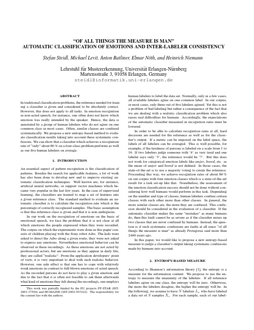
Off all things the measure is man Automatic classification of emotions and inter-labeler co
“OF ALL THINGS THE MEASURE IS MAN”AUTOMATIC CLASSIFICATION OF EMOTIONS AND INTER-LABELER CONSISTENCY Stefan Steidl,Michael Levit,Anton Batliner,Elmar N¨o th,and Heinrich NiemannLehrstuhl f¨u r Mustererkennung,Universit¨a t Erlangen-N¨u rnbergMartensstraße3,91058Erlangen,Germanysteidl@informatik.uni-erlangen.deABSTRACTIn traditional classification problems,the reference needed for train-ing a classifier is given and considered to be absolutely correct. However,this does not apply to all tasks.In emotion recognition in non-acted speech,for instance,one often does not know which emotion was really intended by the speaker.Hence,the data is annotated by a group of human labelers who do not agree on one common class in most cases.Often,similar classes are confused systematically.We propose a new entropy-based method to evalu-ate classification results taking into account these systematic con-fusions.We can show that a classifier which achieves a recognition rate of“only”about60%on a four-class-problem performs as well as ourfive human labelers on average.1.INTRODUCTIONAn essential aspect of pattern recognition is the classification of patterns.Besides the search for applicable features,a lot of work has also been done to develop new and to improve existing au-tomatic classification techniques.Well known are,for instance, artificial neural networks,or support vector machines which be-came very popular in the last few years.In the case of supervised learning,the classifiers are trained to map a set of features into a given reference class.The standard method to evaluate an au-tomatic classifier is to calculate the recognition rate which is the percentage of correctly recognized samples.The basic assumption is that this reference class is given and that it is non-ambiguous.In our work on the recognition of emotions on the basis of emotional speech,we face the problem that it is not clear at all which emotions the people expressed when they were recorded. The corpus on which the experiments were done in this paper con-sists of children playing with the Sony robot Aibo.The kids were asked to direct the Aibo along a given route;they were not asked to express any emotions.Nevertheless emotional behavior can be observed in these recordings.As these emotions are not acted by professional actors,but are emotions as they appear in daily life, they are called“realistic”.From the application developers’point of view,it is very important to deal with such realistic behavior. However,one side effect is that one has to cope with relatively weak emotions in contrast to full-blown emotions of acted speech. As the recorded persons do not have to play a given emotion and due to the fact that it is often not feasible to ask them afterwards what kind of emotions they felt during the recordings,one employs This work was partially funded by the EU projects PF-STAR(IST-2001-37599)and HUMAINE(IST-2002-507422).The responsibility for the content lies with the authors.human labelers to label the data set.Normally,only in a few cases, all available labelers agree on one common label.In our corpus, in most cases,only three out offive labelers agreed.Yet this is not a problem of bad labeling but rather a consequence of the fact that we are dealing with a realistic classification problem which also raises real difficulties for humans.Accordingly,the expectations of the automatic classifier measured in recognition rates must be lowered.In order to be able to calculate recognition rates at all,hard decisions are needed for the reference as well as for the classi-fier’s output.If a metric can be imposed on the label space,the labels of all labelers can be averaged.This is well possible,for example,if the tiredness of persons is labeled on a scale from1to 10.If two labelers judge someone with’8’as very tired and one labeler says only’5’,the reference would be’7’.But this does not work for categorical emotion labels like anger,bored,etc.as the mean of anger and bored is not defined.In those cases,the state-of-the-art is to use a majority voting to create the reference. Proceeding this way,we achieve recognition rates of about60% on our corpus with four emotion classes which is a state-of-the-art result for a task set-up like that.Nonetheless,the assessment of the emotion classification success should not be done without con-sidering how well humans would perform in this task.Depending on the number and type of classes,human labelers confuse certain classes with each other more than other classes.In general,the more similar classes are,the more they are confused.This confu-sion should be considered in the evaluation of a classifier.If the automatic classifier makes the same“mistakes”as many humans do,then this fault cannot be as severe as if the classifier mixes up two classes that are never confused by humans.Instead,the ques-tion is if such systematic confusions are faults at all since“of all things the measure is man”as already Protagoras said more than 2400years ago.In this paper,we would like to propose a new entropy-based measure to judge a classifier’s output taking systematic confusions made by humans into account.2.ENTROPY-BASED MEASUREAccording to Shannon’s information theory[1],the entropy is a measure for the information content.We propose to use the en-tropy to measure the unanimity of the labelers.If all reference labelers agree on one class,the entropy will be zero.Otherwise, the more the labelers disagree,the higher the entropy will be.In the following,we assume to have N labelers L n who have labeled a data set of S samples X s.For each sample,each of our label-ers has to decide in favor of one of K classes C k.However,the approach is also easily portable to soft labels where all classes get scores from a continuous range of values and all scores for a sam-ple sum up to one.The hard decisions of any number of labelers can be converted into one soft reference label as it is depicted in Fig.1for a four-class-problem(K=4)with ten labelers.The more the labelers disagree theflatter is the distribution of the soft label.labeler class1A2E3A4N5A 6E 7A 8A 9N 10E →A M E N0.50.00.30.2Fig.1.Conversion of the hard decisions of ten labelers into a soft reference label l ref.The four classes are’A nger’,’M otherese’,’E mphatic’,and’N eutral’Our suggestion is to leave out each labeler(we can also use a more general term“decoder”)in succession.If labeler n is left out,then the resulting soft reference label for sample X s is denoted l ref(¯n,s),with¯n indicating the omitted labeler.Now,we add another decoder.This can be an automatic clas-sifier,but also the remaining human labeler who was omitted in the reference,so that direct comparisons between a classifier and a human labeler are possible.In order to avoid dependency on the number of labelers,the new decoder is not considered in the same manner as other reference labelers.Instead,the hard decision of the new decoder for sample X s(also converted into a soft label l dec(s))is weighted1:1with the reference label l ref(¯n,s):l(¯n,s)=0.5·l ref(¯n,s)+0.5·l dec(s)(1) Then,the entropy can be calculated for the given sample X s:H(¯n,s)=−Kk=1l k(¯n,s)·log2(l k(¯n,s))(2)Taking the example of Fig.1,the entropy will decrease com-pared to the reference labels if the decoder decides in favor of ’A nger’as’A nger’is what the majority of labelers said.Other-wise,if the decoder chooses’E mphatic’,the entropy will increase but not as much as if the decoder decides in favor of’N eutral’since 30%of the labelers agree that this sample is’E mphatic’and only 20%said the sample is’N eutral’.As none of the labelers decided for’M otherese’,choosing this class yields the highest entropy. This makes sense since’M otherese’seems to be definitely wrong in this case.Note that if using hard decisions,’A nger’would be the only correct class although50%of the labelers disagree.Next step is to average each of the two computed entropy val-ues for X s over the left-out labelers:H(s)=1Nn=1H(¯n,s)(3)We say that our classifier performs not worse than an averagehuman labeler on sample X s,if the entropy from Eq.3with thisclassifier as the new decoder does not exceed the entropy wherethe additional decoders were always humans.By plotting two cor-responding histograms of H(s)for the entire corpus,we obtain avisual means for the assessment of performance of the classifieron this corpus:the closer the histogram for the classifier to the his-togram for the human labelers,the better the classifier.In general,nothing is known about the distributions approximated by thesehistograms.However,if instead of plotting entropy values of in-dividual samples we average them over series of several samples,then,according to the central limit theorem,the resulting distribu-tions will be approximately normal,and thus,describable in termsof its means and variances.In our experiments we used series of20samples.The overall entropy mean itself can be used for comparisonand is computed by averaging H(s)over all samples of the dataset:H=1SSs=1H(s)(4)3.THE AIBO-EMOTION-CORPUSThis entropy-based measure is useful in all those cases where alarge discrepancy between the human reference labelers exists.Inthis paper,we demonstrate the evaluation of different decodersconsidering the example of emotion recognition in speech of chil-dren.All experiments are done on a subset of our Aibo-Emotion-Corpus which consists of51children at the age of10to13years.The children were asked to direct the Aibo robot along a givenroute and to certain objects.To evoke emotions,the Aibo was op-erated by remote control and misbehaved at predefined positions.In addition,the children were told to address Aibo like a normaldog,especially to reprimand or to laud it.Besides that,we pressedthe children slightly for time and put up some danger spots whereAibo was not allowed to go under any circumstances.Neverthe-less,the recorded emotions are relatively weak,especially in con-trast to full-blown emotions of acted speech.The corpus consistsmainly of the four emotions’A nger’,’M otherese’,’E mphatic’,and’N eutral’which were annotated at word level byfive experi-enced graduate labelers.Before labeling,the labelers agreed on acommon set of discrete emotions.For a more detailed descriptionof the corpus,please refer to[2].As’N eutral’is the most frequent“emotion”by far,we downsampled the data until all four classeswere equally present according to the majority voting of ourfivelabelers.At least three labelers had to agree.Cases were less thanthree labelers agreed were omitted as well as those cases whereother than the four basic classes were labeled.In thefinal data set,1557words for’A nger’,1224words for’M otherese’,and1645words each for’E mphatic’and for’N eutral’are used.The inter-labeler consistency can be measured using the kappa statistic.Theformula is given e.g.in[3].For our subset,the kappa value is only0.36which expresses the large disagreement of ourfive labelers.It is generally agreed that kappa scores greater than0.7indicategood agreement.As mentioned above,our low kappa value is notdue to bad labeling.Rather,we are dealing with a difficult classifi-cation problem where even human labelers disagree about certainclasses.4.MACHINE CLASSIFICATION OF EMOTIONS The experiments described in the following are all conducted with artificial neural networks.Because of the small data set,we do “Leave-One-Speaker-Out”experiments:1speaker for testing,40 speakers for training,and10speakers for validation of the neural networks.As features we use our set of95prosodic features and30 part-of-speech features.Details to these features can be found in [4,5].The total number of features is reduced to95using principal component analysis(PCA).Two machine classifiers are trained: machine1is trained with soft labels,machine2with hard labels. The results in terms of traditional recognition rates are given Tab.1 and Tab.2together with a confusion matrix of the classes.The average recognition rate per class is with59.7%slightly higher for machine2which is trained with hard labels than for machine 1which achieves58.1%.The majority voting of allfive labelers serves as hard reference.A M E NΣRRA79147261458155750.8%M5655927582122445.7%E21423947461164557.6%N100941611290164578.4%∅58.1%Table1.Machine decoder1:confusion matrix and recognition rates(RR)evaluated using hard decisions for the classes’A nger’,’M otherese’,’E mphatic’,and’N eutral’A M E NΣRRA89990303265155757.7%M11069768349122456.9%E273431076253164565.4%N215201266963164558.5%∅59.7%Table2.Machine decoder2:confusion matrix and recognition rates(RR)evaluated using hard decisions for the classes’A nger’,’M otherese’,’E mphatic’,and’N eutral’The intention of this paper is to compare those two machine classifiers with an average human labeler as described in Sec.2. But prior to this,we present results for different naive classifiers. In Fig.2(left),entropy histograms for an average human labeler and a random choice classifier,which randomly chooses one of four classes,are shown.As expected,the mean entropy for the simple classifier(1.050,Tab.3)is much higher than for the hu-man labeler(0.722).Accordingly,the histogram of the random choice classifier is shifted to the right.On the right side of Fig.2, the histograms of two other naive decoders are shown.One clas-sifier decides always in favor of’N eutral’,the other one always for’M otherese’.Analyzing the data set,it is obvious that human labelers are often not sure whether they should label a word as emotional or as neutral due to the weak emotions we are dealing with.Consequently,deciding for’N eutral’conforms more to the human labeling behavior than deciding for a certain emotion class. This fact is reflected in our entropy values as well.The mean entropy for the classifier that always chooses’N eutral’is0.843 which is better than random choice.In contrast,always deciding for’M otherese’is quite worse(1.196).decoder entropy measurehuman majority voting0.542human labeler0.721machine10.722machine20.758choose always’N’0.843choose always’E’ 1.049random choice 1.050choose always’A’ 1.127choose always’M’ 1.196Table3.Different decoders and their classification results w.r.t. our entropy measureAs for the comparison between the two machine classifiers, the entropy measure H from Eq.4shows that the decoder machine 1performs as well as an average human labeler,albeit it yields an average recognition rate per class of“only”58.1%.The mean en-tropy is with0.722almost identical with the value attained by the human labelers(0.721).Our second machine decoder machine2, even though it is slightly superior to machine1in terms of recog-nition rates,performs a little worse than it in terms of the mean entropy(0.758).The reason becomes obvious if one looks at the confusion matrices in Tab.1and Tab.2.Both neural networks are trained in such a way that all four classes should be recognized equally well.This works better if hard labels are used for training as in the case of machine2.In contrast,machine1tends to favor ’N eutral’,and this is exactly what humans do in our data set.This is why the entropy measure,being a rather intuitive one,prefers machine1over machine2,even though its recognition rates are lower.The reference for calculating recognition rates is the majority voting of allfive labelers.This majority voting can also be in-terpreted as decoder.In Fig.3(right),this decoder is plotted in comparison with an average human labeler.The mean entropy of 0.542specifies the minimum entropy which can be achieved by a machine decoder.Thus,a machine classifier can very well be bet-ter than a single human on average.The results show that we are as good as one of our human labelers on average,but that there is also enough room for further improvements.5.CONCLUSIONWe proposed a new entropy-based measure which makes possi-ble a comparison between human labelers and machine classi-fiers.Even more important for the evaluation is the fact that sys-tematic confusions of human reference labelers are taken into ac-count as in most of our cases the reference is far from being non-ambiguous.For instance,slight forms of’A nger’are often con-fused with’E mphatic’or with’N eutral’since it is very hard to distinguish among these emotions–even for humans.From the application’s point of view,deciding for a similar class cannot be that wrong in those cases.Our measure punishes classification faults that also occur in human classification less than those faults that are never done by humans.Traditional recognition rates are not capable of this distinction.0.05 0.1 0.15 0.20.25r e l. f r e q u e n c y [%]entropy0.05 0.1 0.15 0.2 0.25r e l. f r e q u e n c y [%]entropyparison between an average human labeler and three naive classifiers:a decoder which selects randomly one of the four classes (left)and two decoders which always choose ’N eutral’and ’M otherese’respectively (right)0.05 0.1 0.15 0.20.25r e l. f r e q u e n c y [%]entropy0.05 0.1 0.15 0.2 0.25r e l. f r e q u e n c y [%]entropyparison between an average human labeler and our machine decoder 1(left)and the majority voting of our five human labelers respectively (right)6.REFERENCES[1] C.E.Shannon,“A Mathematical Theory of Communica-tion,”in Bell System Technical Journal ,vol.27,pp.379–423,623–656.1948,reprint available at /cm/ms/what/shannonday/paper.html (08/17/2004).[2] A.Batliner,C.Hacker,S.Steidl,E.N¨o th,S.D’Arcy,M.Rus-sel,and M.Wong,“‘You stupid tin box’-children interact-ing with the AIBO robot:A cross-linguistic emotional speechcorpus,”in Proc.of the 4th International Conference on Lan-guage Resources and Evaluation (LREC),2004,vol.1,pp.171–174.[3]R.Sproat,W.Black A.S.Chen,S.Kumar,M.Ostendorf,and C.Richards,“Normalization of non-standard words,”in Computer Speech and Language ,vol.15,pp.287–333.2001.[4] A.Batliner,K.Fischer,R.Huber,J.Spilker,and E.N¨o th,“How to Find Trouble in Communication,”Speech Communi-cation ,vol.40,pp.117–143,2003.[5]J.Buckow,Multilingual Prosody in Automatic Speech Under-standing ,Logos,Berlin,2003.。
环境科学与工程专业英语
1环境工程与科学 Environmental Engineering and Science 2环境监测与评价 Environmental monitoring and assessment3温室气体 greenhouse gases 4地表水 the surface water 浅层水 the subsurface water 地下水 the ground water5环境影响评(EIA )environmental impact assessment6臭氧层减少 ozone depletion 7沙漠化 desertification 8点源 point sources 非点源 nonpoint sources 9初级污染物 primary pollutant 次级污染物 secondary pollutant 10光化学烟雾 photochemical smog 11室内污染 indoor air pollution12固体及有害废弃物污染 solid and hazardous waste pollution13生物多样性减少biodiversity loss 14传统决策 traditional decision making 15原生环境 primary environment 次生环境 secondary environment 16不可再生资源 nonrenewable resources 17生态示范区 ecological demonstrate area 18保护林 protection forest 19环境危机 environmental crisis 20环境预测environmental forecasting 21环境效应environmental effect 22环境承载力environmental capacity 23环境演化evolution of environment 24草地退化 grassland degeneration 25水中悬浮物 suspended solids26孔隙水 void water 27岩溶水 karst water 28流域保护 water basin protection 29淡水 fresh water 海水 salt water 30降雨量 amount of precipitation 降雨强度 intensity of precipitation 31 海洋倾倒 ocean dumping 32水力工程 hydro-engineering33水环境功能区 function district of water environment34土壤肥力 soil fertility33土壤酸碱度 soil acidity and alkalinity 36土壤盐渍化 soil salination 37土壤酸化 soil acidification 38缓冲能力 buffer capacity39盐基饱和度 base saturation percentage 40污水灌溉 wastewater irrigation41事后评价 afterwards assessment 42大气扩散 atmospheric diffusion 43而授限度 limits of tolerance 44生命周期评价 life cycle assessment 45慢性毒性实验 chronic toxicity test 46生物富集 bioaccumulation 47生物浓缩 bioconcentration 48生物放大 biomagnification 49边缘效应 edge effect5总悬浮颗粒物 total suspended particulates(TSP) 51化学需氧量 chemical oxygen demand (COD) 52生物化学需氧量 biochemical oxygen demand (BOD)53总有机碳 total organic carbon (TOC ) 54活性碳 active carbon 55萃取剂 extracting agent56有机高分子絮凝剂 organic pdymer flocculant 57固定大气污染源 stationary sources of air pollution移动大气污染源 mobile sources of air pollution 5环境优先污染物environmental priority pollutant 59回归分析 regression analysis 相关分析 correlation analysis 60相关系数 correlation coefficient 61系数误差 systematic error 62随机误差 random error 63土壤修复 soil-remediation 64绝对湿度 absolute humidity 相对湿度 relative humidity 65热辐射 thermal radiation 湍流扩散 turbulent diffusion6煤的综合利用 comprehensive-utilization of coal 67清洁生产 cleaner production 68采矿排水 mining drainage69分子筛吸附NOx 化物过程 control of NOx by adsorption process with molecular sieve70公害 public nuisance 71涡流 eddy current 72富营养化废水 eutrophic wastewater 73富营养化 eutrophication 74中度营养湖泊 mesotrophic lake 75贫营养湖泊 oligotropic lake 76腐殖质化 humification 77土壤质地 soil texture78海水淡化 desalination of seawater 79检出限 detection limit80生态位 niche 81生态型 ecotype 82表面活性剂 surfactant 83光催化作用 photo catalysis84催化作用 catalysis 85格栅 grill86筛网 grid screen 87气浮池 floatation basin 88微电解法 micro-electroanalysis89微生物合成代谢 micro-organism synthetic metabolism90杀菌 sterilization 除味 taste removal 91紫外光消毒 disinfection with ultroviolet vays 93脱臭 odor removal 94脱色decoloration 95污泥浓缩sludge thickening 污泥硝化sludge digestion 污泥脱水sludge dewatering 污泥干燥sludge drying96陆地填埋landfill 97焚烧incineration 98渗滤液处理leachate treatment99最大允许浓度maximum permissible concentration100理境伦理学environmental ethics 101环境适宜度environmental suitability 102排放总量控制total discharge control of pollutant103谁污染谁治理pollutant-treats 104谁开发谁保护explorer-protects105国家级生态示范区national ecological demonstration area106环境管理信息系统information system for environmental management I07环境标记物environmental label 108外部经济性external economics 外部非经济性external diseconomics 109生态足迹the ecological footprint 110代际公平equality between generation 111公众参与public participantion 112回收水系统water reuse system 113绿化用水greenbelt sprinkling 114自然沉降plain sedimentation 115过程水process water116未预见用水量unforeseen water demand 117絮凝沉淀coagulation sedimentation 118垃圾处理sewage disposal 119居民生活垃圾domestic sewage 居民生活污水 domestic water 120市政垃圾municipal sewage121水体自净self-purification of waterbodies 122一级处理primary treatment 二级处理secondary treatment 生物处理biological treatment123活性污泥处理activated sludge process 124污泥焚烧sludge incinerationThe answer to this question requires detailed analyse of local conditions and needs,application of scientific knowledge and engineering judgement based on past experience,and consideration of federal,state,and local regulations. 要解答这个问题首先需要详细的分析当地的实际情况和需求,其次需要应用科学知识和基于经验的工程决断,最后考虑联邦,州和当地法规。
环境影响评价英语

环境影响评价英语Environmental Impact Assessment (EIA) is a process designed to identify and evaluate the potential environmental effects of proposed projects or developments. It helps decision-makers to consider the environmental impacts before making any decisions. The purpose of EIA is to ensure that environmental issues are fully integrated into the decision-making process and that sustainable development is achieved.There are several key steps involved in the EIA process. First, the project is identified and a scoping exercise is carried out to determine the potential environmental impacts that need to be assessed. This is followed by the collection of baseline data to establish the existing environmental conditions. Next, the potential impacts of the project are assessed, taking into account factors such as air quality, water quality, biodiversity, and noise levels. Mitigation measures are then proposed to minimize or avoid any adverse impacts.After the assessment is completed, a report is prepared that summarizes the findings and recommendations. Thisreport is then reviewed by relevant authorities, stakeholders, and the public to ensure that all concerns are addressed. Once any necessary changes have been made, a decision is made on whether to approve the project, with or without conditions.EIA plays a crucial role in ensuring that development projects are carried out in an environmentally responsible manner. It helps to prevent or minimize negative impacts on the environment and promotes sustainable development. By considering environmental factors early in the planning process, decision-makers can make informed choices that benefit both the environment and society as a whole.环境影响评价(EIA)是一种旨在识别和评估拟议项目或发展的潜在环境影响的过程。
classification
classificationClassification is a fundamental task in machine learning and data analysis. It involves categorizing data into predefined classes or categories based on their features or characteristics. The goal of classification is to build a model that can accurately predict the class of new, unseen instances.In this document, we will explore the concept of classification, different types of classification algorithms, and their applications in various domains. We will also discuss the process of building and evaluating a classification model.I. Introduction to ClassificationA. Definition and Importance of ClassificationClassification is the process of assigning predefined labels or classes to instances based on their relevant features. It plays a vital role in numerous fields, including finance, healthcare, marketing, and customer service. By classifying data, organizations can make informed decisions, automate processes, and enhance efficiency.B. Types of Classification Problems1. Binary Classification: In binary classification, instances are classified into one of two classes. For example, spam detection, fraud detection, and sentiment analysis are binary classification problems.2. Multi-class Classification: In multi-class classification, instances are classified into more than two classes. Examples of multi-class classification problems include document categorization, image recognition, and disease diagnosis.II. Classification AlgorithmsA. Decision TreesDecision trees are widely used for classification tasks. They provide a clear and interpretable way to classify instances by creating a tree-like model. Decision trees use a set of rules based on features to make decisions, leading down different branches until a leaf node (class label) is reached. Some popular decision tree algorithms include C4.5, CART, and Random Forest.B. Naive BayesNaive Bayes is a probabilistic classification algorithm based on Bayes' theorem. It assumes that the features are statistically independent of each other, despite the simplifying assumption, which often doesn't hold in the realworld. Naive Bayes is known for its simplicity and efficiency and works well in text classification and spam filtering.C. Support Vector MachinesSupport Vector Machines (SVMs) are powerful classification algorithms that find the optimal hyperplane in high-dimensional space to separate instances into different classes. SVMs are good at dealing with linear and non-linear classification problems. They have applications in image recognition, hand-written digit recognition, and text categorization.D. K-Nearest Neighbors (KNN)K-Nearest Neighbors is a simple yet effective classification algorithm. It classifies an instance based on its k nearest neighbors in the training set. KNN is a non-parametric algorithm, meaning it does not assume any specific distribution of the data. It has applications in recommendation systems and pattern recognition.E. Artificial Neural Networks (ANN)Artificial Neural Networks are inspired by the biological structure of the human brain. They consist of interconnected nodes (neurons) organized in layers. ANN algorithms, such asMultilayer Perceptron and Convolutional Neural Networks, have achieved remarkable success in various classification tasks, including image recognition, speech recognition, and natural language processing.III. Building a Classification ModelA. Data PreprocessingBefore implementing a classification algorithm, data preprocessing is necessary. This step involves cleaning the data, handling missing values, and encoding categorical variables. It may also include feature scaling and dimensionality reduction techniques like Principal Component Analysis (PCA).B. Training and TestingTo build a classification model, a labeled dataset is divided into a training set and a testing set. The training set is used to fit the model on the data, while the testing set is used to evaluate the performance of the model. Cross-validation techniques like k-fold cross-validation can be used to obtain more accurate estimates of the model's performance.C. Evaluation MetricsSeveral metrics can be used to evaluate the performance of a classification model. Accuracy, precision, recall, and F1-score are commonly used metrics. Additionally, ROC curves and AUC (Area Under Curve) can assess the model's performance across different probability thresholds.IV. Applications of ClassificationA. Spam DetectionClassification algorithms can be used to detect spam emails accurately. By training a model on a dataset of labeled spam and non-spam emails, it can learn to classify incoming emails as either spam or legitimate.B. Fraud DetectionClassification algorithms are essential in fraud detection systems. By analyzing features such as account activity, transaction patterns, and user behavior, a model can identify potentially fraudulent transactions or activities.C. Disease DiagnosisClassification algorithms can assist in disease diagnosis by analyzing patient data, including symptoms, medical history, and test results. By comparing the patient's data againsthistorical data, the model can predict the likelihood of a specific disease.D. Image RecognitionClassification algorithms, particularly deep learning algorithms like Convolutional Neural Networks (CNNs), have revolutionized image recognition tasks. They can accurately identify objects or scenes in images, enabling applications like facial recognition and autonomous driving.V. ConclusionClassification is a vital task in machine learning and data analysis. It enables us to categorize instances into different classes based on their features. By understanding different classification algorithms and their applications, organizations can make better decisions, automate processes, and gain valuable insights from their data.。
人工智能与环境科学:智能环境监测与保护

人工智能与环境科学:智能环境监测与保护In the realm of environmental science, the fusion of artificial intelligence (AI) with monitoring and protection systems marks a pivotal advancement towards sustainable practices. AI-driven technologies have revolutionized environmental monitoring by enhancing precision, efficiency, and proactive measures in safeguarding our ecosystems.One of the primary applications of AI in environmental science is intelligent monitoring systems. Traditional methods often struggle with real-time data processing and comprehensive coverage. AI, however, excels in analyzing vast amounts of data from various sources simultaneously. For instance, sensors embedded in ecosystems can continuously gather data on air quality, water levels, and biodiversity. AI algorithms process this data swiftly, detecting patterns and anomalies that human analysts might overlook. This capability allows for early detection of environmental hazards, such as pollutants or habitat disturbances, enabling prompt intervention.Moreover, AI contributes significantly to predictive modeling in environmental conservation. By analyzing historical data alongside current trends, AI can forecast environmental changes and their impacts. This predictive capability aids in planning conservation strategies, such as habitat restoration or species preservation efforts. It also assists in managing natural resources sustainably, optimizing usage based on predicted demand and environmental conditions. Furthermore, AI plays a crucial role in adaptive management practices. Environmental conditions are dynamic and often unpredictable. AI-powered systems can continuously adapt to changing circumstances by learning from new data inputs. This adaptability ensures that conservation efforts remain effective over time, adjusting strategies in response to evolving environmental challenges. In addition to monitoring and prediction, AI enhances the efficiency of environmental protection measures. Automated systems powered by AI can autonomously control variables in industrial processes to minimize environmental footprint. For example, AI can optimize energy consumption in manufacturing or regulate emissions from vehicles based on real-timeenvironmental conditions. Such applications not only reduce ecological impact but also contribute to achieving sustainability goals more effectively.In conclusion, the integration of artificial intelligence with environmental science represents a paradigm shift in how we perceive and protect our natural world. By leveraging AI's capabilities in monitoring, prediction, and adaptive management, we can forge a path towards sustainable development and ecological resilience. As technology continues to advance, so too does our ability to safeguard the environment for future generations.。
数据挖掘课件-分类分析Classification

predicting
Unknown Objects (Without Class Labels)
2
Example: Learning (Training)
3
Example: Testing & Predicting
4
评价指标
预测准确度 计算效率: 建立分类器及预测 对噪音的敏感度 可解读性
5
数据准备
A decision tree is a flowchart-like tree structure, where each internal node (non-leaf node) denotes a test on an attribute, each branch represents an outcome of the test, and each leaf node (or terminal node) holds a class label.
True False
True False
[21+, 5-]
[8+, 30-]
[18+, 33-] [11+, 2-]
16
Entropy
S is a sample of training examples p+ is the proportion of positive examples p- is the proportion of negative examples Entropy measures the impurity of S
分类分析 Classification
1
监督式学习:预测对象的类标签
Training/building
Known Objects (With Class Labels)
白细胞自动分类系统的设计

学术论著 The automatic recognition and classification system for leukocyte not only reduces human consumption, but also improves the detection accuracy and detection speed for Leukocyte classification; MATLAB software; Classifier; System simulation experiment Department of Equipment, Huzhou Third Municipal Hospital, Huzhou 313000, China.作者简介齐天白,男,(1984- ),硕士,工程师。
湖州市第三人民医院设备科,从事医疗器械的临床使用和维护研究工作。
本研究设计一种白细胞自动分类系统,通过模糊模式识别的方法对白细胞进行分类,将显微镜下的模拟图像转换成数字图像,通过对白细胞的分割图像和特征中国医学装备2017年3月第14卷第3期 China Medical Equipment 2017 March V ol.14 No.3学术论著中国医学装备2017年3月第14卷第3期白细胞自动分类系统的设计-齐天白学术论著中国医学装备2017年3月第14卷第3期白细胞自动分类系统的设计-齐天白学术论著中国医学装备2017年3月第14卷第3期白细胞自动分类系统的设计-齐天白学术论著o research and evaluate the application of integrated head-body board in craniospinal irradiation o retrospectively analyze the treatment results of craniospinal irradiation for 43 patients (21 cases were children patients, 0-14 years old; 22 cases were adult patients, >14 years old) used integrated head-body board. During therapeutic process, the registration of the scan image and digitally reconstructed radiograph were applied, which included three parts: head and neck segment, chest segment and lumbosacral segment. And the position errors of X-axe, Y -axe and Z-axe were adjusted by automatic registration. The data of positioning error during the treatment were analyzed by SPSS All of positioning errors in patient using head-body board were less than clinical setting error range(head-neck 0.3cm, body 0.5cm), X direction errors of three segments were (0.122±0.120), (0.074±0.211) and (0.083±0.096)cm, respectively; Y direction errors of three segments were (0.202±0.154), (0.236±0.175) and (0.283±0.187)cm, respectively; Z direction errors of three segments were (0.136±0.127), (0.249±0.472) and (0.272±0.211)cm, respectively; and all of the differences between every positioning error of every segment and corresponding clinical setting error had =-17.814, t =-13.325, 作者简介刘玉连,女,(1988- ),硕士研究生,助理工程师。
Automatic
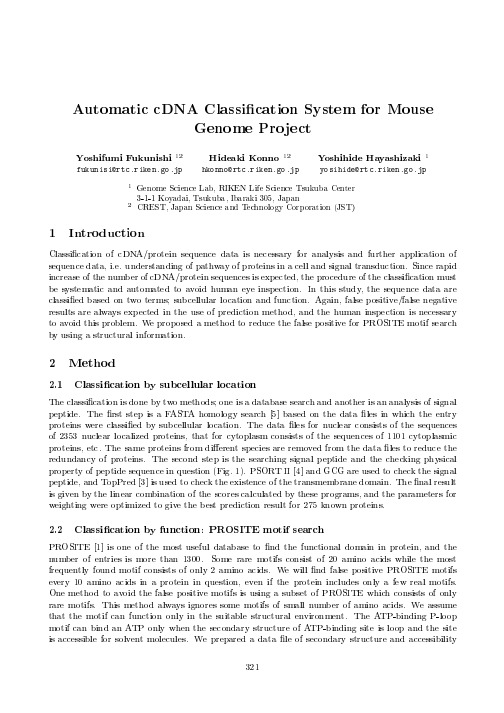
1 Genome Science Lab, RIKEN Life Science Tsukuba Center 3-1-1 Koyadai, Tsukuba, Ibaraki 305, Japan 2 CREST, Japan Science and Technology Corporation (JST)
2 Method
2.1 Classi cation by subcellular location
The classi cation is done by two methods; one is a database search and another is an analysis of signal peptide. The rst step is a FASTA homology search [5] based on the data les in which the entry proteins were classi ed by subcellular location. The data les for nuclear consists of the sequences of 2353 nuclear localized proteins, that for cytoplasm consists of the sequences of 1101 cytoplasmic proteins, etc. The same proteins from di erent species are removed from the data les to reduce the redundancy of proteins. The second step is the searching signal peptide and the checking physical property of peptide sequence in question (Fig. 1). PSORT II [4] and GCG are used to check the signal peptide, and TopPred [3] is used to check the existence of the transmembrane domain. The nal result is given by the linear combination of the scores calculated by these programs, and the parameters for weighting were optimized to give the best prediction result for 275 known proteins.
- 1、下载文档前请自行甄别文档内容的完整性,平台不提供额外的编辑、内容补充、找答案等附加服务。
- 2、"仅部分预览"的文档,不可在线预览部分如存在完整性等问题,可反馈申请退款(可完整预览的文档不适用该条件!)。
- 3、如文档侵犯您的权益,请联系客服反馈,我们会尽快为您处理(人工客服工作时间:9:00-18:30)。
AUTOMATIC CLASSIFICATION OF ENVIRONMENTAL NOISE EVENTS BY HIDDENMARKOV MODELSPaul Gaunard Corine Ginette Mubikangiey Christophe Couvreur Vincent Fontaine Facult´e Polytechnique de Mons,31,Boulevard Dolez,B-7000Mons,BELGIUMTel:++3265374176-Fax:++3265374129Email:couvreur,fontaine@tcts.fpms.ac.beABSTRACTThe automatic classification of environmental noise sources fromtheir acoustic signatures recorded at the microphone of a noise mon-itoring system(NMS)is an active subject of research nowadays.This paper shows how hidden Markov models(HMM’s)can be usedto build an environmental noise recognition system based on a time-frequency analysis of the noise signal.The performance of the pro-posed HMM-based approach is evaluated experimentally for theclassification offive types of noise events(car,truck,moped,air-craft,train).The HMM-based approach is found to outperform pre-viously proposed classifiers based on the average spectrum of noiseevent with more than95%of correct classifications.For compari-son,a classification test is performed with human listeners for thesame data which shows that the best HMM-based classifier outper-forms the“average”human listener who achieves only91.8%ofcorrect classification for the same task.1.INTRODUCTIONThe latest generation of noise monitoring systems(NMS’s)is ba-sed on digital signal processing technology.They commonly im-plement such features as computation and storage of noise levels(),one-third-octave spectra,statistical indices or the detectionof noise events based on thresholds.Since the computational powerof signal processors keeps increasing,it is likely that NMS’s willbecome capable of even more sophisticated treatments of the sounddata they record.Consequently,research has been undertaken todevelop new measurement features for inclusion in NMS’s.An areaof research that has started to attract much attraction recently is au-tomatic noise recognition(ANR).The goal of an ANR system isthe automatic—i.e.,without human intervention—classification ofthe noise sources that are present in the acoustic environment fromtheir recordings at the microphone of the NMS.One particular problem in ANR is the classification of noiseevents such as car or truck pass-bys,aircraftfly-overs,etc.TheANR systems that have been proposed for that task rely generallyon two-step process:a pre-processor converts the acoustical signalof the noise event into a set of characteristic features which are thenused by a classifier to make a decision on the nature of the source ofthe noise event.Until now,the pre-processors that have been pro-posed were based on a“static”approach.That is,the noise eventwas reduced to a global set of characteristics which is then used3.APPLICATION OF HMM’S TO ANRAs the theory of HMM’s is widely described in the literature,we invite the reader who is not familiar with hidden Markov modelingto refer to standard tutorials such as the ones available in[5]or[3].In this paper,five specific types of noise event sources are con-sidered:cars,trucks,mopeds,aircraft,and trains.Because of their transient nature,these types of noise events are well suited to be modeled by left-right HMM’s.Several issues involved in the de-sign of a HMM classifier for this environmental noise event recog-nition application are now discussed.First,a spectral analysis pre-processor must be selected for the classifier and its parameters must be chosen.For the LPC-cepstral analysis pre-processor,the parameters are:the analysis frame length, the analysis frame shift,the order of the LPC model,the num-ber of cepstral coefficients,etc.For thefilter-bank analysis pre-processor,a practical choice would be to use the one-third-octaveor octavefilter-banks with computation of short-time commonly provided by standard sound level meters.Second,it must be decided if a vector quantization step is in-corporated between the spectral analyzer pre-processor and the hid-den Markov model classifier.If VQ is used,it is necessary to de-cide on a codebook size and a distance measure.Finally,the typeof HMM’s that will be used must be selected and their parame-ters(number of states,transition probability matrix structure,etc.) must be chosen.Once the type of HMM and the type of pre-processor have been chosen,taking into account the external constraints,it is still neces-sary tofind the parameter set that will yield the best performance. This can only be done with a combination of trial-and-error experi-ments and engineering experience,possibly guided by some phys-ical understanding of the acoustical phenomena modeled.It is also possible to use the rules-of-thumb for the design of HMM-based classifiers which are used in speech recognition community.4.EXPERIMENTAL RESULTSIn this section,experimental results obtained for the classificationof environmental noise events with hidden Markov models are pre-sented.Five types of noise event sources are considered:cars,trucks, mopeds,aircraft,and trains.The noise event recordings used for the training and the evaluation of the HMM’s are extracted from the MADRAS database.The STRUT software provides the imple-mentation of HMM algorithms.4.1.The MADRAS DatabaseThe MADRAS database of environmental noise sources has been constructed for the MADRAS project which has been partially funded by the European Community and involves several research part-ners in various European countries[2].The aim of the MADRAS project(Methods for Automatic Detection and Recognition of Acoustic Sources)is to develop new noise monitoring instruments with the ability to automatically identify and quantify,in real time,the vari-ous acoustic sources which make up a given acoustic environment. The MADRAS database includes high quality recordings of vari-ous types of common environmental noise sources such as trains, cars,trucks,delivery vans,motorcycles,mopeds,aircraft,chain saws, lawnmoyers,industrial plants,etc.Several instances of each typeof source are provided.The recording conditions of each noise sour-ce are documented.For the classification experiments that will be presented here, onlyfive types of noise recordings available in MADRAS were used: cars,trucks,mopeds,aircraft,and trains recordings.4.2.The STRUT SoftwareThe practical implementation of HMM algorithms is not a trivial programming task.Fortunately,software tools are available that can greatly help the realization of HMM-based classification sys-tems.Our application of hidden Markov modeling techniques to environmental noise event recognition relies on the Speech Train-ing and Recognition Unified Tool(STRUT)developed in the Cir-cuit Theory and Signal Processing(TCTS-Multitel)Laboratory of Facult´e Polytechnique de Mons to conduct research on speech recog-nition[6].STRUT is a software toolbox that consists of many small “independent”pieces of code running on Unix(SUN,HP,Linux) and Windows workstations.Each small program implements a spe-cific step in the speech recognition process:signal pre-processing (extraction of spectral features),vector quantization,Viterbi decod-ing,probability evaluation,maximum-likelihood training,classifi-cation,etc.The small programs communicate by exchangingfiles, through Unix pipes or through Unix sockets.4.3.Classification ResultsThe HMM-based classifiers were trained on a set of noise event recordings extracted from the MADRAS database and the classi-fication performance was evaluated on a distinct set of recordings also extracted from the MADRAS database.The partition of the events of a given type between training and test set was random. The training set contained141noise event recordings:45“car”events,33“truck”events,28“moped”events,14“aircraft”events and21“train”events.The test set contained43noise event record-ings:14“car”events,11“truck”events,9“moped”events,4“air-craft”events and5“train”events.Testing the performance on only 43samples means that the recognition rate estimates will not be very reliable,but it was not possible to use a larger testing set(or training set)because of the limited size of the MADRAS database.In thefirst experiment,the pre-processor was the standard LPC-cepstral pre-processor of speech recognition.The performance of a classifier for the values of the pre-processor parameters commonly used in speech recognition applications was evaluated.The values of the parameters are:analysis frame length30msanalysis frame shift(overlapping factor)set to one third of,order of auto-regressive analysisnumber of cepstral coefficients equal to12VQ codebook size.A three-state HMM was used().The HMM also included three“silence”states at its beginning and at its end.This classifier correctly recognized91%(39/43)of the test samples.In the next series of experiments,the pre-processor was still the LPC-cepstral pre-processor but,this time,parameters of the pre-processor(,)and the number of states of the HMM’s()were varied.Only the most significant results will be presented here.A more complete description of the results obtained can be found in[7].Figure1shows the influence of the analysis frame lengthon the recognition rate for single-state,three-state,andfive-stateR e c o g n i t i o n r a t e (%)Analysis frame length w (ms)Figure1:Effect of the analysis frame length on the recognitionrate forFigure 2:Effect of the order of the autoregressive pre-processor on the recognition rate forHMM’s.All the other parameters are the same as in the first ex-periment.It is observed that the best classification results are ob-tained for frame lengths larger than the standard speech recogni-tion frame length of 30ms:on the order of 50–60ms for three or five-state HMM’s,and 80–100ms for single-state HMM’s.This can be interpreted as an indication that the “typical duration”of the acoustic events and transitions is longer in noise events than in speech.Figure 2shows the influence of the order of the LPC analy-sis on the recognition rate for single-state,three-state,and five-state HMM’s.The frame length was set to 100ms for the single-state HMM’s,to 50ms for the three-state HMM’s,and to 60ms for the five-state HMM’s,respectively.Again,all the other parameters are the same as in the first experiment.The best results are always ob-tained for,the same value as in speech recognition.The codebook size was also varied.Classification results for various combinations codebook sizes ,number of states ,and analysis frame length (in ms)are given in table 1.The best results are al-ways obtained for ,for all analysis frame lengths and forTable 1:Effect of the codebook size on the number of correctclassifications (out of 43)Table 2:Effect of the analysis frame length and number of states on the number of correct classifications (out of 43)for the one-third-octave pre-processor(ms)all number of states tested.Overall,the best performance achieved was 95%(41/43)correct classifications by a five-state HMM with an analysis frame of 50ms or 60ms and with a LPC analysis of order 10used for the pre-processor.In the final series of experiments,the LPC-cepstral pre-proces-sor was replaced by the standard one-third-octave filter bank that is used in noise monitoring applications.In this way,it was possi-ble to investigate the possibility of using a HMM-based as a “post-processor”for a standard sound level meter.Table 2summarizes the results that have been obtained for various analysis frame lengths (integration times for in noise control parlance).The code-book size was again set to 256.The last column ()corre-sponds to a HMM with five states but with only one “silence”state at the beginning and at the end,instead of three.The best perfor-mance achieved was 88%(38/43)correct classification for a three-state HMM and an analysis frame of 100ms or 500ms.4.4.DiscussionEven if the limited size of the MADRAS database means that theperformance numbers obtained must be taken carefully,several con-clusions can still be drawn.First,it appears that HMM-based clas-sifiers outperform simple spectrum-based classifiers.Indeed,HMM-based classifiers yield more than 90%of correct classifications and even more than 95%for the best of them.On the other hand,spec-trum-based classifiers achieve only more than 80%of correct clas-sifications for a similar recognition task on the MADRAS database [2,1].The performance improvement shown by HMM-based classi-fiers could have been expected because the HMM-based classifiers take into account the temporal structure of the noise events unlike the previous spectrum-based classifiers.Second,the analysis frame length is larger in the noise recogni-tion case.This can be interpreted as an indication that the “typical duration”of the acoustic events and transitions is longer in noise events than in speech.Third,it seems that the filter bank-based classifier is outper-formed by the LPC-based classifier.Interestingly,it can be notedTable3:Correct classification by human listenersSound Recognition rate(%)this is also usually the case in speech recognition[3].This can mean that LPC-cepstral analysis is better suited to noise recognition than one-third-octave analysis.However,this could also be due to the fact that thefilter bank pre-processor provides21-dimensional fea-ture vectors before quantization whereas the LPC-cepstral pre-pro-cessor provides12coefficients.It is thus possible that,because of the limited size of the training data,the codebook might not be as well trained in thefilter bank case as it is in the LPC-cepstral case.Finally,it is possible that the limited size of the MADRAS data-base may also have caused training and testing problems.4.5.Listening TestsIn order to get a“baseline”performance level for a human listener, a series of informal listening tests was conducted.In these tests, human subjects were asked to classify noise event recordings into one offive possible categories.The noise event recordings were the same as the one used in the automatic recognition experiments of the previous section.For our experiments,110noise event recordings were extracted from the MADRAS database,with approximately an equal num-ber of“car,”“truck,”“moped,”“aircraft,”and“train”events.The event recordings(WA Vfiles)were played in random order on loud-speakers via the sound board of a PC and a power amplifier.A group of six human listeners was asked to perform the classifica-tion test.The listeners’group included engineers with and without noise control experience.Globally,the listeners correctly classi-fied91.8%of the noise events.Table3breaks down the results by categories of sound.Additional results can be found in[7].Comparing the results obtained by the HMM-based classifiers and the results obtained during the listening test,it appears that, globally,the best classifiers outperform the“average”human lis-tener by a few percents.Lookine more closely at the noise events that were missclassified by human listeners and by HMM-based classifiers,it seems that the sounds that create problems to the HMM classifiers are also often the sounds that create problems to the hu-man listeners.So,in a sense,even when committing a classifica-tion error,the classifier might still make a“perceptually meaning-ful”decision.5.SUMMARY AND CONCLUDING REMARKSIt has been shown how HMM’s could be used to build practical noise classifiers based on a time-frequency analysis of the noise signal.The HMM-based approach to noise recognition has been evaluated experimentally for the classification offive types of noise events(car,truck,moped,aircraft,train).The best results obtained were95.3%of correct classifications for afive-state HMM using LPC-ceptral pre-processsing.For comparison,a classification test has been performed with human listeners for the same data which has shown that the best HMM-based classifier outperformed the “average”human listener who achieves only91.8%of correct clas-sification for the same task.Only discrete HMM’s have been evaluated for the classifica-tion of noise events because they are the simplest type of HMM. It was not possible to evaluate the performance of more complex models such as Gaussian mixtures HMM’s or hybrids neural net-works/HMM’s because there were not enough training data to use these more demanding models.Performance improvment can thus probably be expected once it becomes possible to use these more complex models.For further research,it would be a good thing to increase the size of the MADRAS database.It should contain more samples of each of the variants of the noise events.Research in environ-mental noise recognition would greatly benefits from the creation of large size standardized reusable corpora,like the ones used in speech recognition.6.ACKNOWLEDGMENTThe authors would like to thank Jean Nemerlin of CEDIA for pro-viding access to the MADRAS database.7.REFERENCES[1]P.Chapelle,C.Couvreur and L.-M.Croisez,“ExperimentalResults on Automatic Recognition of Environmental Noise Sources”,ACUSTICA united with acta acustica,vol.82,S1, p.S220,Jan.1996.[2] D.Dufournet and P.Jouenne,“MADRAS,an intelligent as-sistant for noise recognition”,in Proc.INTER-NOISE’97, Budapest,Hungary,Aug.1997.[3]L.Rabiner and B.-H.Juang,Fundamentals of Speech Recog-nition,Prentice-Hall,Englewood Cliff,NJ,1993.[4] A.Gersho and R.M.Gray,Vector Quantization andSignal Compression,Kluwer Academic Published, Boston/Doordrecht/London,1992.[5]L.R.Rabiner,“A tutorial on hidden Markov models and se-lected application in speech recognition”,Proc.IEEE,vol.77,no.2,pp.257–286,Feb.1989.[6]TCTS-Multitel,Facult´e Polytechnique de Mons,Mons,Bel-gium,Step by Step Guide to Using the Speech Training and Recognition Tool(STRUT)–Users’s Guide,Aug.1996, [http://tcts.fpms.ac.be/speech/strut.html].[7]P.Gaunard and C.G.Mubikangiey,“Reconnaissance au-tomatique des bruits environnementaux”,undergraduate the-sis,Facult´e Polytechnique de Mons,Mons,Belgium,June 1996,in French.。