MappingSoilElectricalConductivityUsingOrdinaryKrig
Mapping Watershed Potential to Contribute Phosphorus from Geologic Materials to Receiving Streams

Mapping Watershed Potential to Contribute Phosphorus from Geologic Materials to Receiving Streams, Southeastern United States By Silvia Terziotti, Anne B. Hoos, Douglas A. Harned, and Ana Maria GarciaU.S. Department of the Interior U.S. Geological SurveyOriginally published as Scientific Investigations Map 3102Reformatted to 8 1/2" x 11" page sizeU.S. Department of the InteriorKEN SALAZAR, SecretaryU.S. Geological SurveyMarcia K. McNutt, DirectorU.S. Geological Survey, Reston, Virginia: 2010For more information on the USGS—the Federal source for science about the Earth, its natural and living resources, natural hazards, and the environment, visit or call 1-888-ASK-USGSFor an overview of USGS information products, including maps, imagery, and publications,visit /pubprodTo order this and other USGS information products, visit Any use of trade, product, or firm names is for descriptive purposes only and does not imply endorsement by the U.S. Government.Although this report is in the public domain, permission must be secured from the individual copyright owners to reproduce any copyrighted materials contained within this report.Suggested citation:Terziotti, Silvia, Hoos, A.B., Harned, D.A., and Garcia, A.M, 2010, Mapping watershed potential to contribute phos-phorus from geologic materials to receiving streams, southeastern United States: U.S. Geological Survey Scientific Investigations Map 3102, 1 sheet.ContentsAbstract (1)Introduction (1)Mapping Watershed Potential to Contribute Phosphorus from Geologic Materials (2)Bed-Sediment Phosphorus Concentration Source Data (2)Delineating Geologic Map Units (4)Delineating Areas Affected by Phosphate Mining (6)Characterization of Bed-Sediment Phosphorus Concentration Using Geologic Map Units (7)Characterization of Contribution of Phosphorus to Streams from Geologic Materials Disturbed by Mining Activities (10)Using Regionalized Bed-Sediment Phosphorus Concentration in Watershed Models to Characterize Contribution of Phosphorus to Streams (10)Data Layer Products (12)Acknowledgments (12)Selected References (12)Figures1–2. Map showing—1. Locations of stream sites sampled for bed-sediment phosphorusconcen t rations in the southeastern United States as part of theU.S. Geological Survey National Geochemical Survey. (3)2. Level IV ecoregions and geology in the southeastern United States (4)3. Images showing representations of the areal extent of mined land withina phosphate-mine operation (6)4–6. Map showing—4. Geologic map units for which mean value of bed-sediment phosphorusconcentration was adjusted because of insufficient bed-sedimentsampling sites (8)5. Mean values of bed-sediment phosphorus concentration withingeologic map units. Bed-sediment samples collected from headwaterstreams draining relatively undisturbed areas, 1976–2006 (9)6. Areal extent of phosphate-mined land in the southeastern United Statesand geologic map units that overlap the mined land, with estimates ofbed-sediment phosphorus contribution to streams (11)Tables1. Basin drainage areas and percentages of agricultural land and developed landfor National Geochemical Survey stream sites sampled for bed-sedimentphosphorus content in the southeastern United States (2)2. Data sufficiency classification and methods for assigning averagebed-sediment phosphorus concentrations to geologic mapping units (7)AbstractAs part of the southeastern United States SPARROW (SPAtially Referenced Regressions On Watershed attributes) water-quality model implementation, the U.S. Geological Survey created a dataset to characterize the contribution of phosphorus to streams from weathering and erosion of surficial geologic materials. SPARROW provides estimates of total nitrogen and phosphorus loads in surface waters from point and nonpoint sources. The characterization of the contri-bution of phosphorus from geologic materials is important to help separate the effects of natural or background sources of phosphorus from anthropogenic sources of phosphorus, such as municipal wastewater or agricultural practices. The poten-tial of a watershed to contribute phosphorus from naturally occurring geologic materials to streams was characterized by using geochemical data from bed-sediment samples collected from first-order streams in relatively undisturbed watersheds as part of the multiyear U.S. Geological Survey National Geochemical Survey. The spatial pattern of bed-sediment phosphorus concentration is offered as a tool to represent the best available information at the regional scale. One issue may weaken the use of bed-sediment phosphorus concentration as a surrogate for the potential for geologic materials in the watershed to contribute to instream levels of phosphorus—an unknown part of the variability in bed-sediment phosphorus concentration may be due to the rates of net deposition and processing of phosphorus in the streambed rather than to vari-ability in the potential of the watershed’s geologic materials to contribute phosphorus to the stream. Two additional datasets were created to represent the potential of a watershed to contribute phosphorus from geologic materials disturbed by mining activities from active mines and inactive mines.Mapping Watershed Potential to Contribute Phosphorus from Geologic Materials to Receiving Streams, Southeastern United States Silvia Terziotti, Anne B. Hoos, Douglas A. Harned, and Ana Maria GarciaIntroduction The largest reservoir of phosphorus (P) in the environ-ment is minerals in sedimentary rocks (Mueller and Helsel, 1996). Although, in general, phosphorus compounds in rock minerals are relatively insoluble and do not readily move in runoff or groundwater, erosion of surface soil and rock may be a substantial source of suspended phosphorus in streams in some areas where sedimentary rock is exposed, where soils derived from sedimentary rock exist (Dillon and Kirchner, 1975), or especially where deposits of phosphorus minerals are mined. Phosphate mineral deposits in consolidated material in the southeastern United States generally are of two types—phosphate nodules (oolites, or grains incorporated in sedimentary rocks) and accumulations in residuum derived from the weathering of bedrock (U.S. Geological Survey, 1968). In addition, ore-grade deposits of phosphate minerals are present in formations of large areal extent in Florida and Tennessee (two areas where phosphate output is the largest in the Nation) and in formations of smaller areal extent in North Carolina and Alabama. Data describing phosphate mineral content of ore material are available for many mined areas; however, these data cannot be used to characterize the mass of P contributed from the watershed without additional information on density and distribution of the ore material within the host rock. Phosphorus concentrations in streambed sediment, however, may represent average phosphorus levels in the surficial geologic material of the contributing watershed and delivery of this material to the stream (Cannon and others, 2003). The U.S. Geological Survey (USGS) created a dataset to characterize the potential for a watershed to contribute phosphorus to streams from weathering and erosion of surficialgeologic materials. The motivation for creating this dataset was to support calibration of a phosphorus-transport model (SPARROW—SPAtially Referenced Regressions On Water-shed attributes) for streams in the southeastern United States. SPARROW (Schwarz and others, 2006) provides estimatesof total nitrogen and phosphorus loads in streams from point and nonpoint sources, including background, or naturally occurring, sources. The data also may be useful for a variety of other purposes, including understanding regional background variations in surface-water phosphorus concentrations and developing nutrient criteria.Mapping Watershed Potentialto Contribute Phosphorus from Geologic MaterialsIn order to create a map of bed-sediment phosphorus concentration values that can be applied to the entire Southeast, values of phosphorus were compiled and summarized by geo-logic map units. The source data for phosphorus concentration, the method of deriving geologic map units, and the identifica-tion of phosphorus mine locations are described below.Bed-Sediment Phosphorus Concentration Source DataThe USGS National Geochemical Survey (NGS) compiles data on geochemistry of stream-channel sediment (first-order streams) and soil in order to construct geochemi-cal maps and refine estimates of baseline concentrations of chemical elements (U.S. Geological Survey, 2004). Phospho-rus data are incorporated into the NGS data base primarily from the re-analysis of a subset of samples collected between 1976 and 1980 for the National Uranium Resource Evaluation (NURE) Program (Averett, 1984) and analyses of new samples collected during 1997–1999 and 2004–2006 by the USGS and collaborating State agencies. In the Southeast, the NGS contains nine datasets based on NURE samples (Alabama I, Alabama II, Coastal 98, Coastal 99, Kentucky, South Carolina, 2000, 2002, and 800) for a total of 6,842 samples, and nine State datasets (Alabama, Florida I, Florida II, Georgia, Mississippi I, Mississippi II, States 2006a, States 2006b, and Tennessee) for a total of 3,280 samples (U.S. Geological Survey, 2004). Thus, 10,122 bed-sediment samples were available across the southeastern U.S. for mapping bed-sediment phosphorus concentration (BSPconc; fig. 1).Streams for bed-sediment sampling in the Southeast for the NURE program were selected randomly from topographic maps marked with grids that cover 10 to 30 square kilometers (km2), with an average density of one site per 13 km2.If possible, no sites were selected that were closer than1.5 kilometer (km) to another site, and the area drained was no more than three times the area of the grid so that the maximum size of a basin draining to a site would be 90 km2. The largest headwater stream within the grid was chosen ifthe site was accessible to field personnel (Bolivar, 1980), and an attempt to sample most streams draining from 8 to 26 km2 (3 to 10 square miles) was made (Ferguson and others, 1976). Samples were collected upstream from roads, pondsor other disturbances that could have altered the sampling results, and samples were collected outside of populated areas (Information Systems Programs, Energy Resources Institute, 1985) in order to accurately represent the local-scale variation in sediment mineral composition with surficial geology or other geographical characteristics. In the development of datasets for the NGS, NURE samples in most areas were selected randomly for re-analysis in order to achieve a density of approximately one sample per 289 km2; however, in densely sampled areas in Kentucky and Alabama, all of the NURE samples were re-analyzed.In order to verify that samples were in general from small, undisturbed basins, basin drainage area and watershed percentage of developed and agricultural area at each sampling site in the Southeast SPARROW study area (7,421 of the10,122 sampling sites) were examined using the National Hydrography Dataset Plus (NHDPlus, 2009). The NHDPlus maintains tables that include cumulative drainage area and basin characteristics derived from the 1992 National Land-Cover Data (NLCD; V ogelmann and others, 2001) for every stream segment. Because most samples were taken before 1997, the 1992 land-cover data were most appropriate to use for evaluating anthropogenic effects.Of the 7,421 sampling sites within the SPARROWstudy area, 5,560 could be assigned with confidence (within 200 meters) to an individual stream segment on the 1:100,000-scale NHDPlus. The size distribution of watersheds for these sites confirms that the sites drain small areas; half of the sites drain areas smaller than 9.1 km2 and 90 percent of the sites drain areas smaller than 47 km2 (table 1). Presumably these values would be even lower had all 7,421 sampling sitesbeen included in the analysis; the lack of association withTable 1.Basin drainage areas and percentages of agricultural land and developed land for National Geochemical Survey stream sites sampled for bed-sediment phosphorus contentin the southeastern United States.25th 4.2 2.1018.9 50th9.1120.137.9 75th19.330.50.953.2 90th46.650.3 5.167.2 Mean56.419.2 2.436.92 Mapping Watershed Potential to Contribute Phosphorus from Geologic Materials to Receiving Streams, Southeastern U.S.the 1:100,000-scale NHDPlus that caused 1,861 sites to be excluded from the analysis was, in most cases, due to location of the excluded site on a first-order stream too small for repre-sentation by 1:100,000 hydrography. The distribution of land-cover characteristics of watersheds for the 5,560 sampling sites confirms that the majority of the sites represent basins with little urban development; that is, land cover is less than 0.1-percent developed in half of the watersheds and less than 5-percent developed in 90 percent of the watersheds. Although some of the sites are affected by agricultural activity (land cover is more than 50-percent agricultural for 10 percent of the sites), the majority of the sites are relatively undisturbed (less than 12-percent agricultural in half of the watersheds).sediment BSPconc from this dataset: BSPconc values from the majority of these sites represent conditions with minimal anthropogenic sources in the watershed, and consequently, the average values of BSPconc for different subregions indicate spatial variation in the potential of the upstream watershed to contribute P from naturally occurring geologic materials to the receiving stream channel. • BSPconc values represent the potential contribution of P from the local area adjacent to the sampling site (Bolivar, 1980). • BSPconc values represent streambed conditions in small headwater stream channels. Bed-sediment sampling siteEXPLANATIONA T L A N T I C O C E A NG U L F O F M E X I C OBase modified from U.S. Geological Survey National Elevation Dataset, 100-meter resolutionMapping Watershed Potential to Contribute Phosphorus from Geologic Materials 3Figure 1. Locations of stream sites sampled for bed-sediment phosphorus concen t rations in the southeastern United States as part of the U.S. Geological Survey National Geochemical Survey.Delineating Geologic Map UnitsThe BSPconc values were grouped into geologic map units (GMUs), defined by using regional-scale geologic features, and averaged to a single value for each GMU. The grouping and averaging accomplished two objectives: (1) creating a continuous surface of BSPconc throughout the Southeast regardless of sample-site density, and (2) minimizing the effect of BSPconc values that are affected by human activity. As previously discussed, the site-selection strategy for the bed-sediment data networks in NGS favor sites in relatively undisturbed areas; in practice, however, the BSPconc results at some sites may be affected by anthropogenic sources. Potential bias introduced by these sites was minimized by averaging values from many sites within a GMU.4 Mapping Watershed Potential to Contribute Phosphorus from Geologic Materials to Receiving Streams, Southeastern U.S.Figure 2.(A) Level IV ecoregions (data from U.S. Environmental Protection Agency,Level IV Ecoregions, 1:250,000 scale, 2007) and (B) geology in the south-eastern UnitedStates (data from U.S. Geological Survey, Geologic map of the United States, 1:2,500,000scale, 1974. [Colors are used to illustrate the relative number of distinct classes, not todistinguish individual features].The GMUs were created by delineating zones with similar lithochemistry based on geologic age (King and Beikman, 1974) and geomorphic setting (indicated by level IV ecoregions; U.S. Environmental Protection Agency, 2007). The digital maps of geologic age and level IV ecoregions were overlain and merged to create unique GMUs for each combination of geologic age and ecoregion. This combi n ation creates units with similar geologic properties and accounts for regional variations reflected by ecoregions. Additional boundaries representing known phosphate-rich formations in Tennessee and Florida were incorporated to refine the GMU boundaries in these areas (Smith and Whitlatch, 1940, p. 8, 15;Clawges and Price, 1999; fig. 2).Mapping Watershed Potential to Contribute Phosphorus from Geologic Materials 5Figure 2. (A) Level IV ecoregions (data from U.S. Environmental Protection Agency, Level IV Ecoregions, 1:250,000 scale, 2007) and (B) geology in the south-eastern United States (data from U.S. Geological Survey, Geologic map of the United States, 1:2,500,000 scale, 1974. [Colors are used to illustrate the relative number of distinct classes, not to distinguish individual features].—ContinuedDelineating Areas Affected by Phosphate Mining In this analysis, P derived from geologic material that has been extracted from a subsurface deposit and placed on the land surface was characterized separately from P derived from naturally occurring geologic materials in a watershed. The mapped location and description of phosphate mines from the Mineral Resources Data System (MRDS; U.S. Geological Survey, 2005b) were used to identify all possible areas where disturbed geologic materials may affect instream P concentra-tion. The MRDS dataset contains 839 mine sites, active and inactive, in the southeastern United States. The determi n ation of mine status is based on information from the active mines and mineral plants in the U.S. dataset (U.S. Geological Survey, 2005a), which identifies 19 of the 839 phosphate mines sites as active mines.Only two active mine operations were identified outside of Florida, one in Mississippi and one in North Carolina. Boundaries of mined land for these operations were estimated by using aerial photography (fig. 3A). High-resolution imagery was used to identify the parcels and delineate the boundary for the mined areas.Because delineations of inactive mine operations were not available outside of west-central Florida, and becausethe land use at the inactive mine locations has been altered making it difficult to identify using current aerial photography, an estimate of the area associated with an inactive phosphate mine was based on active mining operations within a GMU. The mean area value of mined land (area classified as barren land in the NLCD (Homer and others, 2004) observed for a subset of mine operations within the GMU was assigned to inactive phosphate mine locations (fig. 3B). For example, inactive mine operations in central Tennessee were assigned a mined-land area of 0.1 km2, whereas inactive mine operations in southwestern Florida were assigned a mined-land areaof 4.3 km2. The areal extent was represented as a circular area centered over the coordinate of the point location (from MRDS), with radius sized to match the assigned area (for example, radii of 35 or 1,171 meters to correspond with assigned areas of 0.004 or 4.3 km2).For mining operations in west-central Florida, boundaries of mined land were estimated by using a combination of geospatial datasets describing location of land parcels and barren land cover (fig. 3C). The Mandatory Phosphate Mine Boundaries geospatial dataset from the Florida Department of Environmental Protection (2007) was used to delineate land parcels identified as inactive and active mining operations. The parcels from this layer were combined with the set of parcels of land disturbed by phosphate mining prior to 1975 (Zellar-Williams, Inc., and Conservation Consultants, Inc., 1980), some of which represent mines that are still active. Areas of actual mining activities within each of these parcels were identified and coded by using the areas classified as barren in the NLCD. For parcels identified by the Mandatory Phosphate Mine Boundaries not included in the Zellar-Williams parcels, only the sections that were classified as barren were considered to represent the areal extent of mined land. For parcels identified by the Zellar-Williams report, which explicitly delineate disturbed land, the entire parcel area (not just NLCD barren land) was used to represent the areal extent of mined land.A B C6 Mapping Watershed Potential to Contribute Phosphorus from Geologic Materials to Receiving Streams, Southeastern U.S.Figure 3.Representations of the areal extent of mined land within a phosphate-mine operation. (A) Basedon aerial photography, active mine delineation in North Carolina (red lines indicate areal extent of mined land); (B) based on average size of barren land polygons within a geologic map unit, inactive mines in Tennessee (yellow lines represent the geologic map unit boundaries); and (C) based on land parcels and barren land cover, active and inactive mines in west-central Florida (red lines indicate areal extent of mined land).Characterization of Bed-Sediment Phosphorus Concentration Using Geologic Map UnitsBy overlaying and merging digital maps of geologic age, level IV ecoregions, and boundaries of local formations, a set of 608 GMUs were delineated for the Southeast. GMUs smaller in area than 30 km 2 were combined with an adjacent GMU to remove the artifact of numerous small units created along the edges of the intersecting map layers. The GMUs with fewer than three stream sites were considered to have insufficient data points to define a representative mean value and, therefore, were classified as “data poor.” The 278 GMUs in the data-poor classification compose only about 8 percent of the study area. An algorithm was developed to compute new values for the data-poor GMU by averaging the data-poor value with the mean BSPconc value from other GMUs with at least one of the following prioritized criteria: (1) GMUs within the same level III ecoregion and of the same geologic age as the data-poor GMU; (2) GMUs with the same geologic age (regardless of ecoregion) and adjacent to the data-poor GMU; or if these first two conditions fail, (3) using BSPconc values from all adjacent GMUs to calculate a mean BSPconc value for the data-poor GMU. A final test was conducted to determine if the new BSPconc value assigned to the data-poor GMU differed by more than 500 parts per million (ppm) from the original GMU BSPconc values. If this was the case, mean BSPconc values using all three conditions were calculated, and the BSPconc value closest to the original value was used. The areal extent and location of the data-poor GMUs are summarized in table 2 and displayed in figure 4, respectively.The spatial pattern in BSPconc was evaluated with respect to the GMU boundaries using one-way ANOV A and the Tukey multiple-comparison test. The GMUsexplained 56 percent of the total variation in BSPconc, and distributions between some GMUs were sufficiently different (at alpha = 0.1) to enable division into distinct groupings. Figure 5 displays the mean BSPconc from phosphorus values of bed-sediment samples collected in undisturbed, headwaterstreams within a GMU .Table 2. Data sufficiency classification and methods for assigning average bed-sediment phosphorus concentrations to geologic mapping units.[GMU, geologic map unit; BSPconc, bed-sediment phosphorus concentration; definition of data sufficiency classification: sufficient—sufficient number of sampling points (three or more) within the GMU to represent the average condition and no adjustments to mean value, poor—insufficient number of sampling points (less than three) to represent the average condition and adjustment to the original mean value was applied; percentages may not add up to 100 because of rounding]Poor24485,6527.9Average the BSPconc of samples from within the GMU with average BSPconc from GMUs in same level III ecoregion that have the same geologic agePoor 263,2790.3Average the BSPconc of samples from within the GMU with average BSPconc from adjacent GMUs with the same geologic age (regardless of ecoregion)Poor 96670.1Average the BSPconc of samples from within the GMU with average BSPconc from adjacent GMUs (regardless of geologic age and ecoregion)Total 6081,083,506100Characterization of Bed-Sediment Phosphorus Concentration Using Geologic Map Units 78 Mapping Watershed Potential to Contribute Phosphorus from Geologic Materials to Receiving Streams, Southeastern U.S.0200300 KILOMETERS100National Atlas, 1:2,000,000 scale, 1972Figure 5.Mean values of bed-sediment phosphorus concentration within geologic map units. Bed-sediment samplescollected from headwater streams draining relatively undisturbed areas, 1976–2006.Characterization of Contribution of Phosphorus to Streams from Geologic Materials Disturbed by Mining Activities During phosphate mining activity, phosphate-rich mineral deposits are disturbed and can affect the concentration of Pin nearby streams. Estimates of the potential of an upstream watershed to contribute P to streams from runoff from areas of disturbed geologic materials can be developed as a simple function of areal extent of mined land in the watershed, or as a combined function of areal extent of the mined land and the level of phosphate enrichment in the mined deposit. Following the second approach, a series of graded step functions was developed by assigning zero for areas mapped as undisturbed and by assigning a gradient of values in disturbed areas that reflects the varying levels of phosphate enrichment in mined deposits. A value for potential was assigned to each mined area in the Southeast by associating the estimated mined-area polygon with the overlapping GMUs. The method may assign a value to a mine based on bed-sediment sampling sites outside the estimated mined-area polygon (fig. 6A, B), depending on the location of the maximum BSPconc in the GMU relative to the polygon.The status of a mining operation was used to weight the value associated to a mine. An active mine is assigned the maximum value within the GMU that its areal extent overlaps, whereas an inactive mine is assigned a value midway between the maximum and mean value of the GMU that its areal extent overlaps. This is illustrated in figure 6C, for a GMU for which the maximum BSPconc for bed-sediment sampling sites is 9,176 ppm and the average BSPconc is 708 ppm. The GMU contains mine polygons that fall in both active and inactive mining activity zones; active mines were assigned the value 9,176 ppm (GMU maximum) and inactive mines were assigned the value of 4,942 ppm (average of 9,176 and 708 ppm).This approach makes two assumptions, both with unknown validity: (1) ore of similar phosphate-mineral content is extracted from mines within the same GMU, and (2) the BSPconc for at least one sample within the GMU reflects the influence of phosphate-mining activity. Estimates of BSPconc therefore, may be less reliable in areas with high density of mined land, as the density of geochemical survey data is insufficient to determine variable loading rates among individual mines or to differentiate contributions from mined-land from contributions from natural, undisturbed land in these ing Regionalized Bed-Sediment Phosphorus Concentration in Watershed Models to Characterize Contribution of Phosphorus to Streams Calibration and application of watershed models of instream transport and concentration of P require characteriza-tion of the potential of the upstream watershed to contribute P from naturally occurring geologic materials in the watershed to instream (water-column) P flux in the receiving stream. For an empirical watershed model such as SPARROW, characterizing potential contribution in absolute mass units is not necessary; rather, characterizing the relative variability, or gradient, of contribution across the region is sufficient. SPARROW’s regression analysis determines the appropriate functional relation between the explanatory variable (for example, BSPconc) and the mass contributed to instream P flux.The spatial distribution of BSPconc from the NGS dataset, which represents headwater streams draining relatively undisturbed watersheds, is useful for modeling the gradient in potential to contribute P to streambed sediments in headwater streams. The response variable of interest in watershed models, however, generally is contribution to instream flux rather than contribution to streambed sediments, and it is not clear that spatial distribution of BSPconc is useful in modeling instream P flux. Instream P flux and BSPconcin headwater streams are influenced by several of the same factors—variation in availability of P in geologic materialsin the watershed and variation in basin rates of erosion and transport of P to the edge of the stream. BSPconc is influenced further by variation in the rates of net deposition and processing of P in the streambed (McDowell and Sharpley, 2001; Walling and others, 2003). The spatial pattern of BSPconc, therefore, is useful as a surrogate for watershed contribution to instream P flux only under the assumptionsof (1) equal rates across all headwater streams in the region, (2) net deposition from the water column, and (3) processing within the streambed sediment. Such assumptions are challenged by known variability among headwater streams in frequency of flushing, occurrence of low dissolved-oxygen conditions, and aquatic-plant processing. The spatial pattern of BSPconc is offered as a tool, representing the best available information at the regional scale, with the caveat that the surrogate relation is weakened by not accounting for variability in headwater streams in the rates of net deposition and processing of P in the streambed.10 Mapping Watershed Potential to Contribute Phosphorus from Geologic Materials to Receiving Streams, Southeastern U.S.。
毕设外文翻译(DOC)

衢州学院本科毕业设计(论文)外文翻译译文:实验室和现场的比较来确定土壤导热系数对能源基金会和其他地下换热器的影响收稿日期:2013年9月10日/接受日期:2014年4月28日在线/发布时间:2014年10月16日©施普林格科学+商业媒体有限责任公司2011年摘要:土壤热导热系数是影响能源基金会和其他地下换热器的一个重要因素。
它可以用现场热响应试验确定,这是昂贵又耗时的,但可以测试大量的土壤。
另外实验室测试法更便宜、更快可应用于较小的土壤样本。
本文研究了两种不同的实验方法:稳态热电池和瞬态探针。
从等会要进行热响应实验的现场采集一个U100土壤试样做一个小直径的测试桩。
试用两种实验室方法测试试样的导热系数。
热电池和探针测的结果明显不同,热电池法测得的导热系数始终高于探针法测得的。
热电池法的主要困难是确定热流率,因为测试设备有显着的热损失。
探针的误差少,但测试的试样比热电池的小。
然而,两种实验室方法得到的导热系数低比现场热响应试验的小得多。
对于存在这些差异的可能原因进行讨论,包括样本的大小,方向和外界干扰。
关键词:能源基金会,探针,热电池,导热系数1 介绍地源热泵系统(GSHP)提供了一个可行的替代传统的加热和冷却系统迈向可持续建筑的解决方案[6]。
热量由制冷剂的装置,它是通过一系列管道埋在地下的泵送在地面和建筑物之间传输。
为了尽量减少初期建设成本,管道可铸造成的基础,消除了需要进一步发掘。
这些系统被称为能量或热的基础。
要设计这样一个系统,它是精确模型的基础与土壤之间的热传递过程中的重要。
这种分析的一个重要的输入参数是土壤热导率。
有几种不同的实验室方法测量土壤热传导率[14,26]。
它们分为两类:稳态或瞬态方法。
在实验室规模,稳态方法涉及施加一个方向热流的试样,然后测量它的输入功率和温度差,当达到稳定状态。
的热导率,然后直接使用傅立叶定律计算。
瞬态方法包括将热施加到样品和监测温度随时间的变化。
Damage detection in CFRP by electrial conductivity mapping

Damage detection in CFRP by electrical conductivity mappingRuediger Schueler a,,,Shiv P.Joshi a ,Karl Schulte b,*aUniversity of Texas at Arlington,Department of Aerospace Engineering,Box 19018,Arlington,TX,76019USAbTechnical University of Hamburg-Harburg,Polymer Composites Section,D-21071Hamburg,GermanyReceived 15April 2000;received in revised form 19April 2000;accepted 20July 2000AbstractCarbon-®ber-reinforced polymer (CFRP)composites derive their excellent mechanical strength,sti ness and electrical coductiv-ity from carbon ®bers.The mechanical deformation and electrical resistance are coupled in these ®bers that make them inherently sensors.Thus CFRPs can be considered as a self-monitoring material without any need for additional sensing elements.However,for this to become reality the conductivity map of the entire structure needs to be constructed and the relationships between the conductivity and various use-and damage-related variables need to be established.Experimental results demonstrate that internal damage,such as ®ber fracture and delamination,decreases the conductivity of composite laminates.In general,the information about the damage size and position can be obtained by utilizing electrical impedance tomography (EIT),but the traditional EIT is not capable of extracting this information when the medium possesses highly anisotropic electrical conductivity.Above a certain level of anisotropy,it is advantageous to modify the traditional EIT.This paper presents a method of extracting the damage size and position for highly orthotropic (unidirectional)CFRPs.The results are obtained without the need for complex calculations,thus enabling damage detection in real time.Experimental observations indicate that a practical EIT has a potential of being a cost-e ective health and usage monitoring technique (HUMT)for CFRPs.#2001Elsevier Science Ltd.All rights reserved.Keywords:Health monitoring;Electrical conductivity;CFRPs;Electrical impedance tomography;D.Non-destructive testing1.IntroductionCarbon-®ber-reinforced polymers (CFRPs)consist of electrically conductive carbon ®bers and a polymeric matrix,which is an insulator.The carbon ®bers are responsible for both the strength and the electrical con-ductivity of the composite material.Thus the sti ness and strength as well as the conductivity is much higher in ®ber direction than in the transverse direction.Many investigators have suggested optical ®bers and other sensors as smart sensing constituents for health and usage monitoring of CFRP laminates.Instead of intro-ducing additional devices into the laminate,our approach suggest that the load-carrying carbon ®bers themselves be utilized for self-monitoring of the CFRP laminates.It is possible to extract the stress/strain ®eld as well as the damage state by mapping the specimen electrical resistivity (or impedance)information.The electrical impedance tomography (EIT)-method gained wide recognition in the 1920s by geophysicists who placed arrays of electrodes into the ground [1,2].Oil-bearing rocks under the surface were identi®ed by injecting current through a pair of electrodes and mea-suring the resulting voltage at other electrodes.In our case,we would like to determine the resistivity distribu-tion in a laminate sheet.A schematic experimental set-up is shown in Fig.1.Various electrodes are connected to the edges of the sample.An electrical current is injected via two electrodes and the potential di erence between all other neighboring electrodes is measured.By taking various combinations of current-injecting electrodes and repeating the potential di erence mea-surements at the remaining electrodes,a wealth of information can be obtained.This information can be utilized to extract resistivity distributions inside the sample using a reconstruction algorithm based on fundamental electrodynamic equations.Once re®ned,the EIT has practical applications in monitoring laminated CFRP structures.The technolo-gical and manufacturing hurdles do not appear to be barrier in implementation of the technique.For example,0266-3538/01/$-see front matter #2001Elsevier Science Ltd.All rights reserved.P I I :S 0266-3538(00)00178-Composites Science and Technology 61(2001)921±930/locate/compscitech*Corresponding author.Tel.:+49-40-42878-3138;fax:+49-40-42878-2002.E-mail address:schulte@tu-harburg.de (K Schulte).,Deceased.by placing electrodes at a one mm spacing along grid lines on a array of size 50mm Â50mm,a detectable damage size is about 5mm (see Fig.2).In existing laminated composite structures,which are often joined together by metal rivets,these rivets can be used as electrodes to measure the resistivity distribution inside a structure.In these structures,the inter rivet distance is typically 25±50mm (1±2inches).From this riveting con®guration,one could expect to detect a damage of size 25mm,if damage is near the rivets.2.Conductivity and damage in CFRPsFor the most part,the conductivity paths follow individual carbon ®bers,since ®bers are surrounded by insulating polymer.Only at inter-®ber contact points can the current switch to an adjacent ®ber.The elec-trical resistance of the specimen is an assemblage of the resistance of all ®bers.Owing to its internal structure,electrical properties of CFRPs are anisotropic.This is especially true for unidirectional laminates.In the ®ber direction (0 direction),the conductivity of the compositeis dominated by the single-®ber conductivity and the ®ber-volume fraction and can be calculated by the rule of mixtures.Perpendicular to the ®bers (90 direction),the conductivity is relatively small.Here,the current transport depends on the existence and number of inter-®ber contact points.This number is related to the ®ber-volume fraction through a percolation process,the waviness of ®bers and ®ber bundles and the amount of misaligned ®bers in a nominally unidirectional laminate.Because of the variation in manufacturing procedures,many di erent values have been reported.A few of them are reported in Table 1.As can be seen,there is a very high anisotropy in the electrical resistivity of CFRP.In literature, 90 / 0 electrical resistivity ratio of 50to about 500are found.Our own measurements on AS4/3501-6yielded an even higher value of 2000.As will be shown later,this high anisotropy makes the applicability of the traditional experimental EIT set-up very di cult.It has been shown by experiments that the resistivity of CFRP increases with the appearance of internal damage,such as ®ber breakage and delamination [12].These experiments proved that the change in electrical resistivity is a viable manifestation of damage in CFRP.The natural extension of this method is a determination of damage class,e.g.®ber breakage or delamination,and damage size and position.However,additional information is needed to quantify these aspects rather then just the gross resistivity change.A promising method for the evaluation of at least the damage size and position is the EIT [3±7].3.Electrical impedance tomographyThere are di erent strategies for collecting experi-mental data for EIT.One of them is the adjacent strat-egy,where current injection is done at two adjacent electrodes (see Fig.1)and the voltage is measured between all other adjacent electrodes.This gives N 2measurements,where N is the number of electrodes,from which N (N À1)/2are independent.The use of the current electrodes is often omitted due to possible con-tact resistance at these points which could be a source of an error.This reduces the number of independentmea-Fig.1.Schematic representation of EIT set-up to a rectangular speci-men using the adjacent data collectionstrategy.Fig.2.Proposed application of EIT to monitor CFRP laminated structures.Table 1Resistivity of CFRPs Material Fiber content (vol.%)0 ( cm)90 ( cm)90 / 0Ref.Carbon/epoxy 550.080.450[8]Carbon/epoxy 650.00251400[9]Carbon/epoxy ±0.00210.95450[10]Graphite/epoxy ±0.062540640[11]AS4/3501-6±0.00362000[12]922R.Schueler et al./Composites Science and Technology 61(2001)921±930surements to N (N À3)/2.For 16electrodes this is equal to 104.We assume that there are no current sources inside the sample,i.e.:div j 3 0A div 6Ágr d 0IIn a two-dimensional case,and if the principal axis of the conductivity tensor coincides with the coordinate axis,this reduces to:@@x x Á@È@x @@y y Á@È@y 0 I Boundary conditions: x Á@È@x y Á@È@yj s P È ÈsPÈ,electric potential; ,conductivity;j s ,current den-sity applied at boundary;Ès ,potential applied at boundary.The governing Eq.(1)is a very complicated di erential equation and it is impossible to obtain its general analytic solution.Thus,a numerical method,the ®nite-element method (FEM),is generally used to derive the solutions.If the conductivity distribution and the boundary conditions j s and Ès are given,the internal potential and current densities can be obtained straightforwardly using Eqs.(1)and (2)and a FEM program.This is called a forward problem.In EIT,instead,we measure the potential and current distributions on the electrodes placed at the boundary of a specimen to determine the internal conductivity distribution.This,so called inverse problem requires many iterative,numerical solutions of a forward problem.In FEM,the domain is divided into a ®nite number of elements and it is assumed that the conductivity in each element is homogeneous.Then,the FEM gives a piece-wise approximation to the governing Eq.(1).This way the di erential equation is transformed into a linear system of equations.Usually,EIT is applied to materials with an isotropic conductivity.CFRP has a highly anisotropic con-ductivity.Therefore,it is necessary to assign at least two conductivity values to each element.The spatial resolu-tion,i.e.the element size,is determined by the maximal number of equations which is equal the number of independent measurements.To give an example:with 16electrodes we get N (N À3)/2=104independent mea-surements.Dividing a quadratic specimen in i x i ele-ments give 2Âi 2unknown conductivity values.This yields i %7which means that each specimen side is divided into seven sections.Doubling the number of electrodes (N =32)gives i %15.An often-used reconstruction algorithm to solve the inverse problem is the Newton±Raphson method.This iterative method minimizes the error F between the measured,V meas ,and estimated potential distribution,V est ( ).F 12V est ÀV me s ÁV est ÀV me sQStarting with an initial guess, 0,the estimatedpotential distribution is calculated using FEM.If the error F is more than a criterion error,the conductivity distribution is altered by Á ,which is a function of V meas ,V est ( )and the derivative V est ( )H .Again,to obtain V est ( )H FEM has to be used.With the improved conductivity distribution the potential distribution and the error are calculated.These steps are repeated until the convergence criterion is met.4.Modi®ed EIT for orthotropic materialsIn the case of low anisotropy,the conventional EIT can be applied to obtain a resistivity distribution of specimen with a minor modi®cation.Until now con-ductivity of only isotropic materials,i.e.independent of direction but position dependent,has been examined using this technique.That means the reconstruction algorithm developed for the isotropic case has to be expanded to account for anisotropy.In practice,the accuracy of this method is limited by the experimental resolution of the potential and current.As will be shown later,this becomes more di cult with increasing anisotropic resistivity ( -ratio),since in this case very small voltages have to be resolved beside large peaks.An arbitrary practical limit for using the tradi-tional EIT method is an estimated -ratio of 100.At high -ratios the traditional data-collection method has to be adjusted.Instead of equidistant electrodes along all four sides,it is advantageous to place the electrodes only along the sides that are perpendicular to the ®ber direction.It is possible to determine the position and the size of a hole in an conductive sheet with a large aniso-tropy (>100).The hole position in a direction transverse to the ®bers could be easily determined by using more ®nely spaced electrodes on sides transverse to the ®ber direc-tion.The position of the hole in the ®ber direction could be obtained by comparing the potential di erence between the electrodes on the current injection side and the electrodes on the opposite side of the specimen.That means a ®ne array of electrodes have to be applied to the specimen,but only on two sides.In contrast,in the case of low anisotropy,electrodes have to be attached to all specimen edges,but with a larger spacing.However,this method has a theoretical limitation as it requires theR.Schueler et al./Composites Science and Technology 61(2001)921±930923shape of the hole(damage)to be known a priori.This requirement is too restrictive for practical implementa-tion of the method.A method to overcome this restric-tion is proposed in the next section.5.Resistor network representationIt is mentioned above that CFRP has a highly aniso-tropic conductivity.It is much higher in the®ber direc-tion than in the transverse direction.Therefore,the approximation of setting the conductivity in the®ber direction to in®nity seems feasible.The procedure to calculate the hole position and size by assuming that the conductivity in the®ber direction (y direction)is in®nite is described below.With this assumption,the sample can be represented by a simple resistor network as shown in Fig.3,where the resistance between two arbitrary electrodes at position x i and x i+1 is given as,i;I 1 Ã x l 1Àx l=a Rwhere a is the specimen dimension in the®ber direction. It should be noted that R represents the product of resistance with the thickness of the specimen.If a hole(or a crack as well)is present in the sample than additional resistors at the hole location have to be introduced as shown in Fig.4.Then the inner resistors R3and R4are given as3=4 Ã d=y u=1 Swhere x is resistivity in x direction,perpendicular to ®bers;d=electrode distance;y u,y1=distance between sample edge and hole edge on upper and lower side, respectively.The outer resistors R0,R7are given as:0 Ã X vÀX0=a S 7 Ã X3ÀX=a SWhere X v,X are the x position of the left and right hole edges,respectively;X i is position of the i th electrode;a is sample height.The other resistors are de®ned by: 1=2 Ã X1E X v=Y u=l Sd 5=6 Ã X E X3=Y u=l SeIn this model,the hole is represented as a rectangle.It is de®ned by its center position(x h,y h)and its widthin Fig.3.Resistor-network representation of a unidirectional CFRPspecimen.Fig.4.Resistor-network representation of an unidirectional CFRP specimen with a hole.924R.Schueler et al./Composites Science and Technology61(2001)921±930longitudinal(h y)and in transverse direction(h x)or equivalently by the position of the left and right edges, x L and x R,and distance between sample edge and hole edge on upper,y U,and lower side,y1.These parameters can be obtained by applying current at four di erent electrode pairs and measuring the voltage response at certain electrodes,which are named below.In experiment,one seeks to avoid the usage of current electrodes for voltage measurements because of the unknown contact resistance.If only one electrode is at the hole position,then only insu cient information can be gained to calculate the values of the six resistors. That means,to calculate the position of the hole in y direction at least two electrode positions(x1and x2) have to be at hole position.Since we examine only symmetric setups(electrodes at both sides have same x positions)as shown in Fig.4,overall eight local elec-trodes(E0..E7)and two at the outer sample edges (EÀI and E+I)have to be considered.The following calculation/procedure can be easily expanded to more electrodes.1.Apply current near left and right edge and mea-sure voltage response at both sides of the intact sample.2.Apply current near left and right edges and mea-sure voltage response at both sides of the sample containing a hole.In comparison with data obtained from the intact sample,the position of the hole in the transverse to the®ber direction can be derived as follows.A voltage increase between an adjacent pair of electrodes indicates that at least a portion of the hole lies with in the area which is between the®ber-direction lines aligned with this pair of electrodes.These pairs of electro-des are utilized for obtaining an accurate estimate of the hole size and position.Fig.8depicts these electrodes as E0±E7.3.Performing three additional sets of measurementusing these electrodes:i.current injection in electrodes E0and E1andmeasurement of voltages U0;1I,U0;123,U0;145,U0;156;ii.current injection in electrodes E1and E2and measurement of voltages U1;2I,U1;256;iii.current injection in electrodes E2and E3 and measurement of voltages U2;3I,U2;301,U2;356,U2;367.Subscripts indicate voltage electrodes,while super-scripts indicate current electrodes.U I is the voltage between two electrodes,iÀI and i I,which are in the regions where the current¯ow and therefore the voltage change is negligible.ÁU1;2I x IdaÀh y@A h y aÀx IdÁU1;2ITFrom these measurements,the hole parameter can bederived by using the formulas:ÁU0;1I x Ix1Àx vaÀh yx vÀx0a@Ax vÁU0;1Ix IÀx1aÀh yx0a1aÀ1aÀh yUÁU2;3I x Ix Àx2ax3ÀxaÀh y@AxÁU2;3Ix IÀx2aÀh yx3a1aÀh yÀ1a: VThe formula to determine the hole position in long-itudinal direction is:y h12a x d13À14Wwhere3U1;256U2;301U2;356U2;367U2;356U1;256U2;356U0;123U0;1561U0;123U0;156U0;145U0;156!Wand4 3U1;256U2;356U0;123U0;156WThe advantage of this outlined procedure to obtainthe hole position and size is that no time-consumingnumerical calculations and iterations are necessary likein the Newton±Raphson-method mentioned in Section3.Thus,the damage detection in real time is possiblewithout super-fast and expensive computers.6.Results and discussionSpecimens made with one ply of the carbon®ber-pre-preg AS4/3501-6were used for experimental investiga-tion.Ply thickness was measured to be0.16mm.Specimens were cut into squares of52mmÂ52mm.Toperform the electrical characterization,16razor bladespressed to the specimen edges every13mm were used aselectrodes(shown in Fig.5).For the data collection,theadjacent strategy was used.An AC current of5mA(2 R.Schueler et al./Composites Science and Technology61(2001)921±930925kHz)was applied to two adjacent electrodes and the potential di erences between all other adjacent electro-des were recorded with a gain of10using an apparatus described elsewhere.After testing the intact specimen,a circular hole,5 mm in diameter,was drilled into the specimen at the desired position.For this the specimen was temporarily disconnected form the electrodes.A two-dimensional,orthotropic sheet with uniform anisotropic conductivity was numerically analyzed.Its size was chosen to be4cmÂ4cm representing a uni-directional ply.Corresponding to our experimental ®ndings of 0O=3Â10À3 cm and 90 =6 cm and a ply thickness of0.015cm,the resistivity in0 -and90 directions were set to0.2and400,respectively,i.e.ani-sotropy ratio=2000.To parametrically study the e ect of various anisotropy ratios the resistivity in0 direction was increased.Resistivity in transverse direction was kept400,resistivity in the®ber direction was adjusted to account for various -ratios.The ANSYS5.3program was used for the®nite-ele-ment calculation.The element type was thermal-electric solid(PLANE67)with four nodes.The global element size was0.0625units,so that the edge space between electrodes is divided into16elements.The model shown in Fig.5includes16electrode positions,1.0cm apart along the specimen edges.Damages to the specimen were modeled by setting the resistivity of damaged regions to1020.These regions were square shaped with an edge length of0.5cm.The potential at the origin of the coordinate system was set to0and a current of 5Â10À3Amp was applied between two adjacent nodes. As mentioned before,a -ratio up to2000was mea-sured in unidirectional CFRP specimen.The e ect of such an anisotropy is shown in Fig.6.Here,the poten-tial distribution is presented when a current of5mA is applied between the electrodes2and3( -ratio=500).It can be seen that all equipotential lines are almost parallel to the®ber direction.This means that the potential drop along the®ber direction is negligible compared to the transverse direction.Thus,resolving the small voltages between,e.g.electrodes5and6is very di cult because it is likely to fall within the noise present in the experi-mental measurements.Finite-element calculations for an intact specimen with a -ratio of2000and experimental results are shown in Fig.7.For various adjacent current electrode pairs the voltage between all other adjacent electrodes are displayed.As can be seen most measurements are negligible compared to the few peaks obtained in90 direction.In Fig.8numerical as well as experimental results for a specimen with a hole in the center(hole1),at the right side(hole2)and at the top(hole3)are shown.The positions of these holes are shown in Fig.5.Experi-mental results are presented with voltage ampli®ed by a factor of10.For clarity,only the di erence in potential between the damaged and the intact specimen is pre-sented.In each case,only one measurement is sig-ni®cantly di erent from the others.For hole1and hole 3this is,when current is applied between the electrodes 2and3and the voltage is measured between10and11. For hole2,the peak shift to the current electrodes3±4 and potential electrodes9±10.These peaks indicate the hole position in90 direction.Peaks for holes1and3 reveal that the entire holes are between x=1.5and x=2.5,whereas the peak for hole2shows that entire hole is between x=2.5and x=ing moreelectrodes Fig.5.2D-Model used for®nite-elementcalculations.Fig.6.Calculated potential distribution of a square specimen,when acurrent of0.005A is applied between electrodes2and3(see Fig.5). 926R.Schueler et al./Composites Science and Technology61(2001)921±930with smaller distances,the hole position transverse to the ®ber direction could be easily determined accurately.The peak height provides information about the amount of conductivity drop in the `examined specimen section'.For instance,by applying current at electrodes 2and 3and measuring the voltage between electrodes 10and 11,this section would be the rectangle spanned between these corners (2±3±10±11).For the intact spe-cimen the voltage is 0.482compared to 0.518with hole 1.That means the conductivity decreased by 7%.In fact,we reduced the conductive area by the hole size,which is about 6%.As this rough estimate shows,the height of the di erence peak indicates,in fact,the con-ductivity drop.The hole position in 0 -direction is still required to be determined.Since specimens with holes 1and 3show the same peak no distinction can be made (see Fig.8).The potential di erence between electrodes 10and 11does not provide enough information to calculate the hole position in 0 direction,90 direction and the hole size.Therefore,the determination of the potential dif-ference between electrodes 10and 11on a ®ner scale is needed.As we saw in Fig.6most information about the specimen is located between electrodes 10±11and 2±3.The di erence in the potential curve between speci-mens with holes and the intact specimen is shown in Fig.9.Current was applied between electrode 2(x =2.5)and 3(x =3.5).The di erences of these curves are accentuated in the derivatives of these curves (see Fig.10).When the hole is in the middle of the specimen,the potential curves which are determined on the current electrode side and on the opposite side are identical.If the hole moves toward the opposite side (holes 4and 3)the peak decreases on the current electrode side.Simul-taneously the peak on the opposite side increases and form adjacent minima.After obtaining a calibration curve,the exact hole position can be revealed from these data.Further,it can be noticed that the width of the peaks is almost the same as the width of the holes.These results are obtained with a priori knowledge of the shape of the hole.The resistor network representation method is described in this paper to overcome this restrictive assumption.However,this method is applic-able to highly orthotropic material.To check the accuracy of the resistor network repre-sentation method,the data from FEM calculations were used.First,a square hole in orthotropic plates with resistivity-ratios of 2000,00,100and 20,respectively,was analyzed.Second,the in¯uence of hole shape and the electrode position was examined.The center of the hole was arbitrarily chosen to be x h =1.5and y h =2.5.The width and height was set to h x =h y =0.5.That means the hole lies between x =1.25and x =1.75.The electrodes were placed at x =1.0625,1.3125, 1.4626,and 1.8125.The electrodes are not placed symmetric with respect to the hole center c =1.5.A symmetric arrangement of electrodes is a special case that will always give the exact x location of the hole.Table 2shows that down to a -ratio of 100the cal-culated parameters are close to the actual values used in the FEM calculation.With further decreasing ratios,the hole height h y ,tends to decrease while the hole width h x increases.This results in a relatively constant hole size with only about 2%di erence from the actual value of 0.25.Below a ratio of 100the error,especially in long-itudinal position y h ,increases signi®cantly.Here the assumption of an in®nite conductivity in longitudinal direction is not valid any more.Until now,only rectangular holes have been con-sidered.In reality one has to deal with holes of an aspect ratio bigger than 1,and holes that are not aligned either to the y -or x -axis.To account for such situations the hole shape shown in Fig.11was used for the FEM cal-culation.The -ratio is again 2000.Two di erent sets of electrodes were examined.First the same set as used before (x 0,x 1,x 2,x 3in Fig.11)and one shifted 0.125cm to the right (x 0H ,x 1H ,x 2H ,x 3H ).Thus the in¯uence of the electrode position has beenevaluated.Fig.7.(a)Finite-element calculation for an intact specimen;(b)experimental results for an intact CFRP specimen.R.Schueler et al./Composites Science and Technology 61(2001)921±930927Fig.8.Numerical (a,c,e)and experimental results (b,d,e)for specimen with hole in the center (a,b),at the right side (c,d)and at the top (e,f).928R.Schueler et al./Composites Science and Technology 61(2001)921±930。
物理勘探方法 英语
物理勘探方法英语Physical Exploration Methods.Physical exploration methods are geophysical techniques that utilize physical properties of the Earth's materials to investigate subsurface structures and properties. These methods involve measuring and interpreting physical fields, such as gravity, magnetic, electrical, and seismic waves, to determine the physical characteristics and geological formations beneath the Earth's surface.Gravity Exploration.Gravity exploration is based on the principle that the Earth's gravitational field varies due to the different densities of subsurface materials. Denser materials, such as metallic ores or massive rocks, exert a stronger gravitational pull than less dense materials, such as voids or fluids. Gravity surveys involve measuring the variations in the Earth's gravitational field using gravimeters. Thesemeasurements can reveal subsurface structures, such as faults, folds, and intrusions, as well as the presence of dense ore bodies or fluid-filled cavities.Magnetic Exploration.Magnetic exploration utilizes the Earth's magneticfield and the magnetic properties of subsurface materials. Magnetic surveys measure variations in the Earth's magnetic field caused by the presence of magnetic minerals or magnetized rocks. Magnetic anomalies, which are deviations from the normal magnetic field, can indicate the presence of magnetic ore deposits, buried metallic objects, or geological structures with contrasting magnetic susceptibilities.Electrical Exploration.Electrical exploration methods involve introducing electrical currents into the ground and measuring the resulting electrical field. The electrical properties of subsurface materials, such as conductivity, resistivity,and dielectric permittivity, vary depending on their composition and porosity. Electrical surveys can detect subsurface structures, such as conductive ore veins, resistive bedrock, and fluid-saturated zones.Seismic Exploration.Seismic exploration is based on the propagation of seismic waves through the Earth's materials. Seismic surveys involve generating seismic waves using controlled explosions or vibrating sources and recording the waves as they travel through the subsurface. The velocity and reflection patterns of seismic waves provide information about the subsurface geology, including the depth, thickness, and composition of rock layers, as well as the presence of faults and hydrocarbon reservoirs.Other Physical Exploration Methods.In addition to the main methods described above, there are various specialized physical exploration methods that can be used for specific purposes. These include:Radioactive Exploration: This method measures the natural radioactivity emitted by radioactive minerals, such as uranium and thorium, to identify radioactive ore deposits.Electromagnetic Exploration: This method utilizes electromagnetic waves to detect conductive subsurface structures, such as ore bodies and buried pipelines.Ground-Penetrating Radar (GPR): This method uses high-frequency electromagnetic waves to investigate shallow subsurface structures, such as buried utilities, cavities, and archaeological remains.Thermal Exploration: This method measures subsurface temperatures to identify geothermal resources, such as hot springs and magma chambers.Borehole Geophysics: This method involves logging down boreholes to obtain physical measurements, such as density, resistivity, and seismic velocity, for detailed subsurfacecharacterization.Applications of Physical Exploration Methods.Physical exploration methods have a wide range of applications in various fields, including:Mineral exploration: Identifying and assessing ore deposits of metals, minerals, and hydrocarbons.Hydrogeological investigations: Determining groundwater resources, assessing aquifer properties, and detecting groundwater contamination.Engineering geology: Evaluating subsurface conditions for construction projects, such as tunnels, dams, and pipelines.Environmental investigations: Identifying buried waste sites, monitoring groundwater contamination, and assessing soil stability.Archaeological surveys: Locating buried structures, artifacts, and archaeological features.Geothermal exploration: Identifying potential geothermal reservoirs for energy production.Advantages and Limitations of Physical Exploration Methods.Physical exploration methods offer several advantages:Non-invasive: These methods do not require direct excavation of the ground, which minimizes environmental impact and disruption.Depth penetration: Some methods, such as seismic and gravity surveys, can provide information about deep subsurface structures.Quantifiable data: The measurements obtained from physical exploration surveys can be quantified and processed to provide detailed subsurface models.However, physical exploration methods also have limitations:Resolution: The resolution of physical exploration methods varies depending on the method and the subsurface conditions.Interpretation: The interpretation of physical exploration data requires expert knowledge and experience to accurately determine subsurface structures and properties.Cost: Physical exploration surveys can be relatively expensive, especially for large-scale projects.。
土壤含水率和盐分对土壤电导率的影响_孙宇瑞
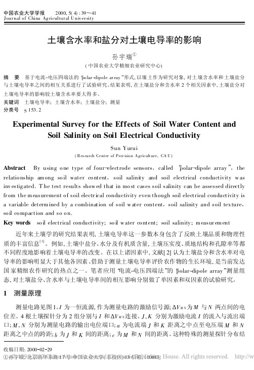
中国农业大学学报 2000,5(4):39~41 Jour nal o f China Ag ricultur al U niv er sity 土壤含水率和盐分对土壤电导率的影响孙宇瑞¹(中国农业大学精细农业研究中心)摘 要 基于电流-电压四端法的“po lar-dipole ar ray”形式,以壤土作为研究对象,对土壤含水率和土壤盐分与土壤电导率之间的相互关系进行了试验研究。
结果表明,在土壤盐分和含水率2个相关因素中,土壤盐分对土壤电导率的影响较土壤含水率要大得多。
关键词 土壤电导率;土壤含水率;土壤盐分;测量分类号 S153.2Experimental Survey for the Effects of Soil Water Content and Soil Salinity on Soil Electrical ConductivitySun Yurui(Res earch Center of Precision Agriculture,CA U)Abstract By using o ne type of four-electrode sensors,called“polar-dipole array”,the relatio nship am ong so il water co ntent,soil salinity and soil electrical conductivity w as inv estig ated.T he test results show ed that in mo st cases soil salinity can be assessed directly fr om the m easurement o f soil electr ical conductivity even though soil electrical conductivity is a variable determ ined by a combination of soil w ater content,soil salinity and soil tex ture, so il co mpaction and so o n.Key words so il electrical conductivity;so il w ater co ntent;soil salinity;m easur em ent近年来土壤学的研究结果表明,土壤电导率这一参数本身包含了反映土壤品质和物理性质的丰富信息[1]。
Testing the performance of spatial interpolation techniques
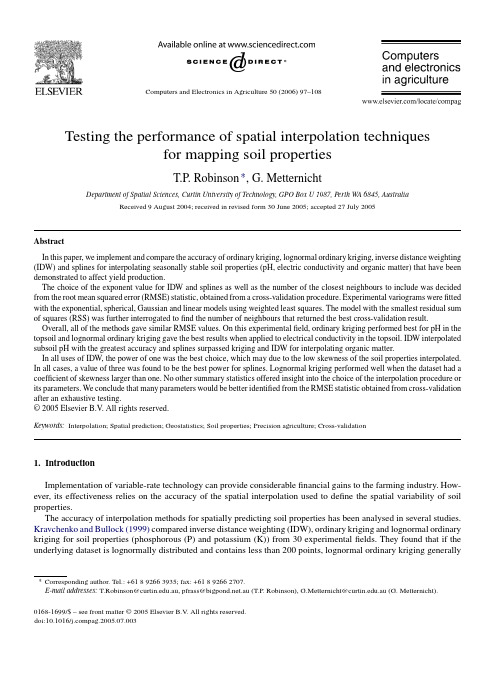
Computers and Electronics in Agriculture 50(2006)97–108Testing the performance of spatial interpolation techniquesfor mapping soil propertiesT.P.Robinson ∗,G.MetternichtDepartment of Spatial Sciences,Curtin University of Technology,GPO Box U 1987,Perth WA 6845,AustraliaReceived 9August 2004;received in revised form 30June 2005;accepted 27July 2005AbstractIn this paper,we implement and compare the accuracy of ordinary kriging,lognormal ordinary kriging,inverse distance weighting (IDW)and splines for interpolating seasonally stable soil properties (pH,electric conductivity and organic matter)that have been demonstrated to affect yield production.The choice of the exponent value for IDW and splines as well as the number of the closest neighbours to include was decided from the root mean squared error (RMSE)statistic,obtained from a cross-validation procedure.Experimental variograms were fitted with the exponential,spherical,Gaussian and linear models using weighted least squares.The model with the smallest residual sum of squares (RSS)was further interrogated to find the number of neighbours that returned the best cross-validation result.Overall,all of the methods gave similar RMSE values.On this experimental field,ordinary kriging performed best for pH in the topsoil and lognormal ordinary kriging gave the best results when applied to electrical conductivity in the topsoil.IDW interpolated subsoil pH with the greatest accuracy and splines surpassed kriging and IDW for interpolating organic matter.In all uses of IDW,the power of one was the best choice,which may due to the low skewness of the soil properties interpolated.In all cases,a value of three was found to be the best power for splines.Lognormal kriging performed well when the dataset had a coefficient of skewness larger than one.No other summary statistics offered insight into the choice of the interpolation procedure or its parameters.We conclude that many parameters would be better identified from the RMSE statistic obtained from cross-validation after an exhaustive testing.©2005Elsevier B.V .All rights reserved.Keywords:Interpolation;Spatial prediction;Geostatistics;Soil properties;Precision agriculture;Cross-validation1.IntroductionImplementation of variable-rate technology can provide considerable financial gains to the farming industry.How-ever,its effectiveness relies on the accuracy of the spatial interpolation used to define the spatial variability of soil properties.The accuracy of interpolation methods for spatially predicting soil properties has been analysed in several studies.Kravchenko and Bullock (1999)compared inverse distance weighting (IDW),ordinary kriging and lognormal ordinary kriging for soil properties (phosphorous (P)and potassium (K))from 30experimental fields.They found that if the underlying dataset is lognormally distributed and contains less than 200points,lognormal ordinary kriging generally∗Corresponding author.Tel.:+61892663935;fax:+61892662707.E-mail addresses:T.Robinson@.au,pfrass@.au (T.P.Robinson),G.Metternicht@.au (G.Metternicht).0168-1699/$–see front matter ©2005Elsevier B.V .All rights reserved.doi:10.1016/pag.2005.07.00398T.P.Robinson,G.Metternicht/Computers and Electronics in Agriculture50(2006)97–108outperforms both ordinary kriging and IDW;otherwise,ordinary kriging is more successful.Further,Laslett et al. (1987)also found ordinary(isotropic)kriging to be a better method than IDW for interpolating pH.In fact,Laslett et al.(1987)judged splines to be a better than both IDW and kriging.In contrast,Gotway et al.(1996)observed better results than kriging for soil organic matter and nitrogen when using IDW.Weber and Englund(1992)also found that IDW produced better results than kriging(with lognormal kriging outperforming ordinary kriging).There have been many conflicting reports concerning the use of basic statistics to predetermine both interpolation methods and their parameters.For example,Kravchenko and Bullock(1999)report a significant improvement in accuracy of soil properties interpolated using IDW by manipulating the exponent value.They found that data with high skewness(>2.5)were often best estimated with a power of four(five out of eight datasets)and for most of the soil properties with low skewness(<1),a power of one yielded the most accurate estimates(9out of15datasets). Alternatively,Weber and Englund(1994)report that IDW with a power of one resulted in a better estimation for data with skewness coefficients in the range of four to six when interpolating blocks of contaminant waste sites.Likewise, a larger exponent produced better estimations when the data had low skewness.For organic matter,in particular,Gotway et al.(1996)found that the accuracy of the inverse distance method increased as the exponent value increased.Theirfindings show that properties with a low coefficient of variation (<25%)were better explained by a higher power,in most cases a power of four.In addition,datasets with a high coefficient of variation gave best results when a power of one was used.On the contrary,Kravchenko and Bullock (1999)found no significant correlation between the exponent value used for IDW and the coefficient of variation.Given the variability of results obtained by these previous studies the research reported hereafter aims to:-Assess the accuracy of various well-known interpolation techniques for mapping soil pH,electrical conductivity and organic matter through manipulation of the various parameters attributable to each technique;-Determine if non-spatial statistics could assist in determining the best interpolation method to implement without using exhaustive test parameters;-Identify the spatial prediction method that best illustrates the spatial variability of the soil properties studied.This would enable the identification of areas where remediation is required to improve crop growth.2.Spatial prediction methods2.1.KrigingThe presence of a spatial structure where observations close to each other are more alike than those that are far apart(spatial autocorrelation)is a prerequisite to the application of geostatistics(Goovaerts,1999).The experimental variogram measures the average degree of dissimilarity between unsampled values and a nearby data value(Deutsch and Journel,1998),and thus can depict autocorrelation at various distances.The value of the experimental variogram for a separation distance of h(referred to as the lag)is half the average squared difference between the value at z(x i) and the value at z(x i+h)(Lark,2000b):ˆγ(h)=12N(h)N(h)i=1[z(x i)−z(x i+h)]2(1)where N(h)is the number of data pairs within a given class of distance and direction.If the values at z(x i)and z(x i+h) are autocorrelated the result of Eq.(1)will be small,relative to an uncorrelated pair of points.From analysis of the experimental variogram,a suitable model(e.g.spherical,exponential)is thenfitted,usually by weighted least squares, and the parameters(e.g.range,nugget and sill)are then used in the kriging procedure.2.2.Inverse distance weightingSimilar to kriging,inverse distance weighting directly implements the assumption that a value of an attribute at an unsampled location is a weighted average of known data points within a local neighborhood surrounding the unsampledT.P .Robinson,G.Metternicht /Computers and Electronics in Agriculture 50(2006)97–10899Fig.1.Study area location and map of the distribution of soil samples.location.The formula of this exact interpolator is (Burrough and McDonnell,1998):ˆz (x 0)= n i =1z (x i )d −r ijn i =1d −rij(2)where x 0is the estimation point and x i are the data points within a chosen neighborhood.The weights (r )are related to distance by d ij ,which is the distance between the estimation point and the data points.The IDW formula has the effect of giving data points close to the interpolation point relatively large weights whilst those far away exert little influence.The higher the weight used the more influence points close to x 0are given.2.3.SplinesSplines consist of polynomials,which describe pieces of a line or surface,and they are fitted together so that they join smoothly (Webster and Oliver,2001).Splines produce good results with gently varying surfaces,and thus are often not appropriate when there are large changes in the surface values within a short horizontal distance.3.Materials3.1.Study area and sampling designThe study area is a 60ha paddock,called ‘Ardgowan ’on a dry land sheep and cropping farm,located in the Shire of Wickepin,in the South West of Western Australia.As a result of ongoing research activities in the application of remote sensing to agriculture,100soil samples were collected at 10and 30cm depth (Fig.1),geo-referenced using a GPS receiver (accuracy of ±5m)and analysed for organic matter,electrical conductivity and soil anic matter was assayed using the ‘loss on ignition’method.A pH electrode was used to measure pH in a 1:1mixture of soil to calcium chloride solution.Electrical conductivity was measured in a 1:5extract.The sampling design was based on slope (derived from a digital elevation model (DEM))and the change in the normalised difference vegetation index (NDVI).The NDVI was derived from a high-resolution digital multispectral image,acquired at 2m spatial resolution.The intent of this strategy is that areas with the greatest change in NDVI coupled with relatively steep slope characterise areas of high variability,which equates to heterogeneous soil properties.Therefore,more sample points were taken over areas with higher variability (Drysdale,2001;Drysdale et al.,2002).3.2.Description of soil propertiesAcidity is a soil property that has a devastating effect on crop growth,because acidification causes a reduction in the availability of some essential nutrients (e.g.calcium and molybdenum)and also an increase of other nutrients to100T.P.Robinson,G.Metternicht/Computers and Electronics in Agriculture50(2006)97–108toxic levels(e.g.manganese and aluminium)(Charman,2000).Soils with a pH less than4.5in CaCl2in the topsoil (0–10cm)are considered toxic to most crops(Fenton and Helyar,2000).These soils,especially where the rainfall is over500mm,often present acidity problems further down the soil profile,and so the subsoil(10–30cm)also requires assessment.If only the topsoil is affected then lime can be incorporated with good results.However,if the entire profile is affected then even an application of lime will still not allow crops to develop deep-root systems.In this case,the pH in the lower levels will improve over several years(depending on the porosity of the soil)as the lime moves down the profile.In general,soils with a pH of between5and7.5present no problems.A pH above9 indicates that salinity and sodicity are likely,although not all sodic and saline soils are alkaline(Fenton and Helyar, 2000).The cause of rising acidity is generally related to nitrate leaching and a build-up of organic anic matter build-up is often the result of pasture improvement procedures such as the application of fertilisers,and the break down of dead soil organisms and plant residues.Nitrate leaching is heavily induced when produce is removed from the paddock,because the surface is exposed and leftover nitrogen is not absorbed by plants(Charman,2000).Lit-erature reviewed states that soils with organic matter contents greater than2.6%have good nutrient storage(Purdie, 1998).Electrical conductivity(EC)of a soil solution can be used to estimate the salinity of an area.Charman(2000) recommend that saline soils are those with an EC greater than1.5dS/m for a1:5extract.More precisely,the yield of most plants is not restricted until the EC is greater than2dS/m(Charman,2000).4.Research approach4.1.Visualization and exploratory data analysisFig.2summarises the methods and techniques applied in this research for spatial prediction and comparative evaluation of the soil properties.This begins with a visual analysis by screening the data values to identify incorrect coordinate information and illogical data points.Visualization is also used to quickly identify the presence or absence of spatial autocorrelation.Description of the data values is achieved via basic summary statistics,including means, medians,variances and skewness.Further exploration is available through histograms,box-plots and normal plots. These tools are useful for examining the values for outliers,which are detrimental to spatial prediction.The variogram, in particular,is very sensitive to outliers because it is based on the squared differences among data(Lark,2000a).The worst effect is when the outlier is near the centre of the study area,as it contributes to the average many times for each lag.If the data are irregularly sampled,as in this study,the relative contributions of the extreme values are even less predictable.The result is that the experimental variogram is not inflated equally over its range,and thus can appear erratic(Webster and Oliver,2001).4.2.Data transformation and interpolationGeostatistical analysis is best performed on Gaussian distributions.When non-normality is apparent,transformations of the data can assist to make it approximately normal.Skewness is the most common form of departure from normality. If a variable has positive skewness,the confidence limits on the variogram are wider than they would otherwise be and as a result,the variances are less reliable.A logarithmic transformation is considered where the coefficient of skewness is greater than1and a square-root transformation if it is between0.5and1(Webster and Oliver,2001).Applying ordinary kriging to logarithmic transformed data is the essence of lognormal kriging.It is important to note that for logarithmic transformations,the back transformation through exponentiation tends to exaggerate any error associated with interpolation,with extreme values the worst affected.To mitigate this effect,we use an unbiased back-transform as shown in Eq.(3)(Deutsch and Journel,1998).ˆz(x i)=expˆγ(x i)+σ2(x i)2(3)whereσ2(x i)is the corresponding lognormal kriging variance,ˆγ(x i)the lognormal kriging estimate andˆz(x i)is the corresponding back-transformed result in the original data domain.T.P.Robinson,G.Metternicht/Computers and Electronics in Agriculture50(2006)97–108101Fig.2.Conceptual model for spatial prediction of soil properties.WLS,weighted least squares;RSS,residual sum of squares;RMSE,root mean squared error found from cross-validation;IDW,inverse distance weighting.4.3.Sample size requirements for variogram computationLiterature suggests some100–150data is the minimum requirement to achieve a stable variogram(e.g.V oltz and Webster,1990).This quota is satisfied in this research,with100data available for each soil property.Due to the need of over300samples to properly detect anisotropy,it is not feasible to explore directional effects for the dataset used in this research.Accordingly,the spatial variation is assumed isotropic and all variograms are omnidirectional.4.4.Criteria for comparisonIt is common practice to use cross-validation to validate the accuracy of an interpolation(V oltz and Webster,1990). Cross-validation is achieved by eliminating information,generally one observation at a time,estimating the value at that location with the remaining data and then computing the difference between the actual and estimated value for each data location(Davis,1987).Cross-validation is an excellent scheme for solving the inconvenience of redundant data collection(Olea,1999;Webster and Oliver,2001),and hence all of the collected data can be used for estimation. The cross-validation technique is used to choose the best variogram model among candidate models and to select the search radius and lag distance that minimises the kriging variance(Davis,1987;Olea,1999).It is also used to assist finding the best parameters from those tested for IDW(Tomczak,1998)and splines.To compare different interpolation techniques,we examined the difference between the known data and the predicted data using the mean error(Eq.(4)),the root mean squared error(Eq.(5)),the average kriging standard error(Eq.(6)), the root mean square standardized prediction error(Eq.(7))and the mean standardized prediction error(Eq.(8)).Eqs.102T.P.Robinson,G.Metternicht/Computers and Electronics in Agriculture50(2006)97–108(6)–(8)are only applicable to kriging as they require the kriging variance.Eqs.(4)and(5)are applicable to all of the interpolation techniques applied in this research.ME=1NNi=N{z(x i)−ˆz(x i)}(4)RMSE=1NNi=1{z(x i)−ˆz(x i)}2(5)AKSE=1NNi=1σ2(x i)(6)RMSP=1NNi=1MEσ(x i)2(7)MSPE=1NNi=1MEσ2(x i)(8)whereˆz(x i)is the predicted value,z(x i)the observed(known)value,N the number of values in the dataset andσ2is the kriging variance for location x i(Johnston et al.,2001;Webster and Oliver,2001;Kravchenko and Bullock,1999; V oltz and Webster,1990).The mean error should ideally be zero,if the interpolation method is unbiased.The calculated ME,however,is a weak diagnostic for kriging because it is insensitive to inaccuracies in the variogram.The value of ME also depends on the scale of the data,and is standardized by dividing by the kriging variance to form the MSPE.An accurate model would have a MSPE close to zero.If the model for the variogram is accurate,then the RMSE should equal the kriging variance,so the RMSP should equal1.If the RMSP is greater than1,then the variability in the predictions is being underestimated,and vice versa.Likewise if the average kriging standard errors(AKSE)are greater than the root mean square prediction errors(RMSP),then the variability is overestimated,and vice versa(Johnston et al.,2001;Webster and Oliver,2001).5.Implementation and discussion of results5.1.Data visualizationFig.3a shows the spatial distribution of the topsoil pH,classified into quartiles,depicting that the bulk of the data have a critical pH range of4.40–4.75.The classified map of subsoil pH(Fig.3b)exhibits a good degree of autocorrelation with similarly classified values clustering together in space.Fig.3c shows the spatial distribution of topsoil electrical conductivity,which illustrates that generally,the paddock does not seem to have a salinity problem in the topsoil(all values less than2dS/m).Fig.3d shows the spatial distribution of the topsoil organic matter with several clusters in the study area.It also appears that much of the paddock has satisfactory levels of organic matter.5.2.Summary statistics,outlier detection and transformationA statistical summary of the pH,EC and organic matter soil properties is presented in Table1.A histogram,box-plot and normal plot were constructed for all soil properties,revealing two outliers for pH.Their removal reduced the coefficient of skewness from0.859to0.266avoiding the need for data transformation.Exploratory analysis suggested one outlier for subsoil pH(4.45),which was removed.Two potential outliers with an EC of0.35and0.4were found from exploratory analysis for electrical conductivity.The bulk of the data has an EC of0.1,which dramatically affects the normality of the distribution.However,it is those values that‘appear’as outliers in the data that are of most interest to the analysis of salinity and hence,they are kept in the dataset.Furthermore,since the coefficient of skewness isT.P.Robinson,G.Metternicht/Computers and Electronics in Agriculture50(2006)97–108103Fig.3.Samples classified by quartiles for(a)topsoil pH,(b)subsoil pH,(c)topsoil electrical conductivity and(d)topsoil organic matter.greater than1(1.761),the natural logarithm is applied for a kriging analysis(thus,lognormal kriging)to stabilise the variance(Goovaerts,1999).This was later back-transformed using Eq.(3).Exploration of organic matter revealed one potential outlier(9%),however,visualization showed that this value is located on the periphery of the paddock and therefore it will not be included in many lags.It also has relatively large values contiguous to it.Consequently,the decision was to include the data in the analysis.Although the coefficient of skewness for organic matter is located inTable1Summary statistics for pH,electrical conductivity(EC)and organic matter(OM)Soil property N Min Max Range Mean Median Var CV(%)Skewness Kurtosis pH(10cm)100 3.95 5.7 1.75 4.596 4.550.0860.859 2.044 pH(30cm)100 4.45 6.6 2.15 5.811 5.850.1757−0.6240.272 EC(dS/m)(10cm)10000.40.40.1340.100.00555 1.761 3.341 OM(%)(10cm)98a 1.9997.01 4.376 4.24 1.983320.610.238a Two samples cracked under laboratory conditions and were not tested.104T.P.Robinson,G.Metternicht/Computers and Electronics in Agriculture50(2006)97–108Table2Summary of the residual sum of squares(RSS)statistic produced for each different modelSoil property RSSTopsoil(10cm)pHExponential0.000215Spherical0.000284Linear0.000847Gaussian0.000228Subsoil(30cm)pHExponential0.000956Spherical0.001260Linear0.025700Gaussian0.001220Topsoil(10cm)electrical conductivity(dS/m)Exponential0.000003Spherical0.000003Linear0.000011Gaussian0.000003Topsoil(10cm)organic matter(%)Exponential0.000157Spherical0.000202Linear0.004400Gaussian0.000336Bolded RSS values were chosen as the best model.Fig.4.Fitted variograms for soil properties.(a)pH in the topsoil(10cm depth)is best represented by the exponential model,which shows a nugget (C0)of0.0539;a sill(C0+C)equal to0.1079;range(A0)equal to2110;coefficient of determination(R2)of0.419;a residual sum of squares(RSS) equal to0.00021.(b)Fitted variogram of pH in the subsoil(30cm depth).(c)Fitted variogram of the electrical conductivity soil property in the topsoil.(d)Fitted variogram of the organic matter soil property in the topsoil.T.P.Robinson,G.Metternicht/Computers and Electronics in Agriculture50(2006)97–108105 Table3Parameters found when the kriging model returned the lowest cross-validation RMSE for all soil propertiesSoil property Neighbours ME RMSE AKSE RMSP MSPETopsoil(10cm)pH25−0.001070.24750.25310.9799−0.00218 Subsoil(30cm)pH300.0013250.3870.3487 1.0920.00247 Topsoil(10cm)EC(dS/m)15−0.00018790.071880.06902 1.0410.004407 Topsoil(10cm)OM(%)50.0004648 1.438 1.363 1.0450.003325ME,mean error;RMSE,root mean squared error;AKSE,average kriging standard error;RMSP,root mean square standardized prediction error; MSPE,mean standardized prediction error.the range where a square-root transformation is appropriate,it is that outlying value on the periphery that is skewing the data,so we chose to leave the data in its original form.5.3.Interpolation and interpretationOmnidirectional experimental variograms for all properties were calculated using Eq.(1).The exponential,spherical, Gaussian and linear models werefitted to the experimental variogram and the model with the lowest residual sum of squares(RSS)was chosen as optimal.Table2summarises the RSS for eachfitted model for all soil properties.The bestfitting models for all of the soil properties are presented in Fig.4.The variogram of topsoil pH(Fig.4a)appears to exhibit a pure nugget effect,which may be because of too sparse a sampling to adequately capture autocorrelation. There is no clear range and sill,nor is the nugget variation small compared to the spatially dependent random variation. It is perhaps inappropriate tofit any model to this experimental variogram.Nonetheless,the exponential model was implemented as it returned the bestfit.Fig.4b shows thefitted variogram for subsoil pH,depicting the range to be around138m(95%of the sill).The exponential variogram model provided the bestfit to the experimental variogram. The experimental variogram for electrical conductivity(Fig.4c),appears erratic and without a distinct structure.The spherical model provided the bestfit to this sequence of data.The experimental variogram for organic matter appears to have quite good structure and a gradual approach to the range,with the exponential model providing the bestfit.The number of closest samples chosen varied from5to30,with afive-sample interval.The best-found kriging parameters were selected from the cross-validation results(Table3).For topsoil pH the lowest root mean square error (RMSE)was found with a neighborhood of25points.The mean error(ME)and mean standardized prediction error (MSPE)suggests that the predictions are relatively unbiased.Since the average kriging standard error(AKSE)is greater than the RMSE,the kriging variance is larger than the true estimation variance and indicates that the variogram model is overestimating the variability of the predictions.The root mean square standardized error(RMSP)also suggests the same since it is less than1.With reference to Fig.4a,it is likely that the RMSP is less than1because thefitted Table4Parameters returning the lowest RMSE from cross-validation for IDW and splines for all soil propertiesSoil property Power Neighbours ME RMSETopsoil(10cm)pHIDW125−0.00770.2485 Splines325−0.00330.252 Subsoil(30cm)pHIDW115−0.0032580.3808 Splines330−0.00280.3839 Topsoil(10cm)EC(dS/m)IDW130−0.0015690.07391 Splines330−0.00010.0735 Topsoil(10cm)OM(%)IDW115−0.03093 1.438 Splines315−0.0134 1.43 ME,mean error;RMSE,root mean squared error;EC,electrical conductivity;OM,organic matter.106T.P.Robinson,G.Metternicht/Computers and Electronics in Agriculture50(2006)97–108exponential model exceeds the observed variances(shown by the squares)at short lags,particularly thefirst lag(and also the third,fifth and seventh),and it is these lags that dominate the kriging systems(Webster and Oliver,2001).The lowest RMSE was found using30nearest neighbours for subsoil pH.The ME and MSPE suggests that the predictions are relatively unbiased.Given that the AKSE is smaller than the RMSE,the variability is being underpredicted.Since the RMSP is greater than1,the kriging variance is smaller than the true estimation variance, possibly a result of the fourth lag in Fig.4b being underestimated by the exponential model.For topsoil electrical conductivity,the most favourable number of neighbours was found to be15.The low values ME and MSPE suggest that the predictions are relatively unbiased.Given that the average standard errors are smaller than the RMSE,the variability is being underpredicted,though not significantly(difference of0.003).Five neighbours were found to be optimal for organic matter.The RMSP is greater than one,and hence the variability is being under-predicted to a small extent.IDW was estimated with powers of one,two,three and four.The precision of IDW is also affected by the choice of the number of the closest samples used for estimation;hence,this was varied from5to30for the various powers used.Fig.5.Interpolated soil maps(a)topsoil pH using kriging,(b)subsoil pH using IDW,(c)topsoil EC using lognormal kriging and(d)topsoil OM using splines.T.P.Robinson,G.Metternicht/Computers and Electronics in Agriculture50(2006)97–108107 Cross-validation was used tofind the best agreement between the measured data and the IDW estimates.In all cases, the best weighting parameter was found to be one.This suggests that the weights diminish slowly from the sample point over the chosen radius.Linear,quadratic and cubic splines were implemented using the same neighborhood variation as used for kriging and IDW.In all cases,the best exponent value was found to be three(cubic splines)suggesting that lower order polynomials were insufficient at representing the variation on the paddock.The best cross-validation parameters for IDW and splines are shown in Table4.The interpolated maps of all soil properties using the method with the lowest RMSE from the cross-validation process can be seen in Fig.5.Fig.5a shows an interpolation of topsoil pH using ordinary kriging.The lowest pH values(and therefore highest acidity)occur on the middle to upper Western side of the paddock with pH values below4.5(critical).The highest pH is located in a large circular‘hole’to the Southeast of the paddock.This map would be useful at directing a differential liming application to lift pH.According to the kriged estimates,the entire paddock has a pH lower than5,which means that crops that are sensitive to acidity will have trouble establish-ing in these soils,resulting in a poor production.Furthermore,since the pH is below5.2(and rainfall is greater than500mm per annum)for the entire paddock there is likely to be a net movement of acidity down to the next layer of the soil(Fenton and Helyar,2000,p.234)and hence it was necessary to examine the subsoil pH.IDW proved to be the best method for interpolating subsoil pH,and the soil map is shown in Fig.5b.Subsoil pH does not show signs of acidic conditions at present with all pH values above5.In this case,a farmer would likely apply sufficient lime to the topsoil to lift the pH of the soil,without the need to wait for the lime tofilter through to the subsoil over time.This would enable crops to establish and develop root systems that are adequate for long-term survival.Fig.5c shows the interpolation of electrical conductivity using lognormal kriging.It reveals that there are no topsoil salinity problems on the paddock,as all values are lower than1.5dS/m.Fig.5d shows the interpolation of organic matter over the paddock using the splines technique.Since a value greater than2.6%suggests good nutrient storage capacity,it can be seen that much of the paddock soil has sufficient organic matter.6.ConclusionsThis study has shown that,out of the four spatial prediction methods used,there is not one single interpolator that can produce chief results for the generation of continuous soil property maps all of the time,particularly with a dataset that has not been designed with one particular interpolator in mind.Overall,all of the methods gave similar RMSE values,using the cross-validation technique for evaluation.Ordinary kriging performed best for pH in the topsoil and lognormal kriging outperformed both IDW and splines for interpolating electrical conductivity in the topsoil.The IDW technique interpolated subsoil pH with the greatest accuracy,and splines surpassed kriging and IDW for interpolating organic matter.In all implementations of IDW the power of one was the best choice(over powers of two,three and four),which is possibly due to the relatively low skewness inherent in all soil properties modelled(as also found by Kravchenko and Bullock,1999).For our dataset,the coefficient of variation could not be used to identify the best a priori weight to use for IDW.The best exponent value for splines was found to be three for all implementations of the splines technique, suggesting lower order polynomials could not capture the variation of the soil properties across the paddock.Lognormal kriging,by stabilising the variance outperformed IDW and splines for the EC dataset,and thus in this research it was found to be a suitable choice when the coefficient of skewness was larger than1.No other summary statistics were found to correlate to any of the parameters chosen after extensive trials.Especially in cases where sampling is not tailored to a particular interpolation technique,summary statistics should not be solely relied upon to infer an interpolation method or interpolation parameters.Instead,whilst the cross-validation technique is not a confirmatory tool,as an exploratory tool it greatly assists in choosing appropriate interpolation procedures and their associated parameters.AcknowledgementsThis research has been supported by the Australian Research Council(ARC),under the Strategic Partnership with the Industry Scheme(SPIRT).The authors also thank Georgina Warren and Jacob Delfos for the collection of the soil samples.Additionally,we acknowledge industry partners SpecTerra Systems Pty Ltd.and the Department of。
翻译

8.2 千瓦的蒸发器,一个装置了一系列长 1.5 米、内径 0.0015 米毛细管的膨胀 装置组成。除此之外,系统有三个独立的流程,即: (ⅰ)地面耦合流程(盐水 循环或者水-防冻液循环) , (ⅱ)制冷剂循环(或者说是一个可逆的蒸汽压缩循 环) , (ⅲ)居民采暖的风机盘管线路(水循环) 。系点要素的主要特点将会在表 一中给出,在表一中括号内的数字对应于图一中所描绘的这些元件。
������������������������������ ������������������������������
������������������������������ ������������������������������ +������������������������������������ +������������������
(8a) (8b)
������������������������������������ =
表一:住宅式地源热泵系统的主要特点
主回路 制冷剂回路 (1-4)
元件 压缩机 (Ⅰ)
技术规范 类型:密闭,往复式;制造商: 特库姆塞;型号: TFH4524 F; 体积流量:7.5 立方米/小时; 速度:2900/分钟;电动机额定 功率: 2HP (1.4 千瓦) , 制冷剂: R-22;容量:4.134 千瓦(蒸发 /冷凝温度为 0/45℃);
析会提供一个综合性的评估。 正如先前所指出的那样, 能源转换装置的花销通常被认为是根据能源本身而 定的。 调查者们根据炯开发出了跟多种经济学分析方法,这些分析方法有很多共 同点: (ⅰ) 他们把炯与经济学规律相结合来提高或者优化它们的经济学性能 (ⅱ) 他们认为炯才是一个系统中商品的价值,而不是能源,于是他们相关的炯变量分 配了成本或者是价格。 作者在以往的文献中对不同进水温度及参考值的地源热泵系统的能源与炯 效率值也做了介绍,这项研究和早期的研究的不同之处如下: (ⅰ)地源热泵系 统是在 EXCEM 的基础上进行建模和分析的; (ⅱ)评估炯经济参数。从这个层面 上看,这里所说的是一个有着额定直径 32 毫米、50 米长的 U 型管地下换热器的 地源热泵系统, 这个系统被设计后安装于土耳其伊兹密尔 Ege 大学的太阳能研究 所。除此之外,我们也从事了一些参数的研究来探索 0-25℃范围内不同的参考 温度是如何影响地面耦合热泵系统的炯经济学分析的, 并提供了可以预测系统热 力学损失在资金成本中所占比例的相关关系。 炯经济学分析也表明我们可以在运作过程中考虑着改善它的热力学性能, 但 仅仅是经济学分析可以决定系统性能改善的可能性与便利性。 这项研究简要的描 述了一个安装在土耳其伊兹密尔 Ege 大学太阳能研究中心的住宅式地源热泵系 统易于遵循的程序, 以及如何通过熵损失计算来将这个程序应用于采暖系统性能 的评估,从而进一步的为性能改善指明了方向。从这些结果中我没回发现,系统 会产生最大的熵损失,尤其是在遇到有电力、机械、和等熵面等效率的影响下, 而且更应强调的是由于性能劣质的组件会很大程度的降低整个系统的工作性能, 所以我我们在设备选型的时候需要给予密切的关注。 这里所介绍的分析结果预计 对那些处理地源热泵系统炯经济学评估的人会带来一些帮助。 2.EXCEM 分析法在住宅式地源热泵系统中的应用 2.1:系统研究的简介 图一演示了本实验的设置图。 为了避免系统中用于冷却的水在工作条件下和冬 季冷冻,就在里面加入了重量 10%的乙基乙二醇的混合物。制冷剂是在闭路铜质 管道中循环的, 该工作流体是 R-22 型。住宅式地源热泵系统是一个空气/制冷剂 蒸汽压缩热泵,主要由一个 1.4 千瓦的压缩机,一个 6.66 千瓦的冷凝器,一个
土壤电导率英文

土壤电导率英文Soil Electrical ConductivityAs a content creator, understanding soil electrical conductivity is an essential component in agriculture and environmental sciences. Soil electrical conductivity refers to the ability of an agricultural soil to conduct electrical currents. It measures the soil's capability to conduct electricity and correlates it to the salt concentration in that soil.Factors Affecting Soil Electrical ConductivitySeveral factors affect soil electrical conductivity,including climatic elements such as precipitation and temperature, soil texture, the amount of organic matter in the soil, and soil salt concentration. Generally, soils that have high salt concentrations result in high soil electrical conductivity, whereas soils with low salt concentrations have low soil electrical conductivity.Applications of Soil Electrical ConductivitySoil electrical conductivity has several applications in the field of agriculture and environmental sciences. It helps farmers in soil salinity management by selecting salt-tolerant crops to plant in soils with high salinity levels. Soil electrical conductivity can also help fertilization management. If a soil has a low electrical conductivity, itmay lack essential nutrients, which can imply that the farmer must increase the fertilizer application rate.Soil electrical conductivity may also be used in environmental assessments. High soil electrical conductivity is often a sign of soil contamination. By measuring soil electrical conductivity, environmental scientists canpinpoint contaminated areas and implement remediation.Measurement of Soil Electrical ConductivitySoil electrical conductivity can be measured using electrical conductivity meters. The tool measures the electrical resistance of the soil, and from that measurement, the electrical conductivity of the soil can be calculated. Two types of electrical conductivity meters exist, contact and non-contact meters. Contact meters require the insertion of the meter into the soil, while non-contact meters are placed on top of the soil surface.Soil electrical conductivity is an essential component in agriculture and environmental sciences. By understanding its applications, measurement techniques, and affecting factors, we can design better soil management strategies and environmental assessments.。
- 1、下载文档前请自行甄别文档内容的完整性,平台不提供额外的编辑、内容补充、找答案等附加服务。
- 2、"仅部分预览"的文档,不可在线预览部分如存在完整性等问题,可反馈申请退款(可完整预览的文档不适用该条件!)。
- 3、如文档侵犯您的权益,请联系客服反馈,我们会尽快为您处理(人工客服工作时间:9:00-18:30)。
Chin. Geogra. Sci. 2019 V ol. 29 No. 2 pp. 270–282Springer Science Press https:///10.1007/s11769-019-1027-1 /content/1002-0063Received date: 2017-11-29; accepted date: 2018-03-14Foundation item: Under the auspices of the National Natural Science Foundation of China (No. 41571217), the National Key Research and Development Program of China (No. 2016YFD0300801)Corresponding author: HUANG Yuanfang. E-mail: yfhuang@© Science Press, Northeast Institute of Geography and Agroecology, CAS and Springer-Verlag GmbH Germany, part of Springer Na-ture 2019Mapping Soil Electrical Conductivity Using Ordinary Kriging Com-bined with Back-propagation NetworkHUANG Yajie 1, LI Zhen 1, YE Huichun 2, ZHANG Shiwen 1, 3, ZHUO Zhiqing 1, XING An 1, HUANG Yuanfang 1(1. Key Laboratory of Arable Land Conservation (North China ), Ministry of Agriculture/Key Laboratory of Agricultural Land Quality Monitoring, Ministry of Land and Resources , College of Resources and Environmental Sciences , China Agricultural University , Beijing 100193, China ; 2. Key Laboratory of Digital Earth Science , Institute of Remote Sensing and Digital Earth , Chinese Academy of Sci-ences , Beijing 100094, China ; 3. School of Earth and Environment , Anhui University of Science and Technology , Huainan 232001, China )Abstract: Accurate mapping of soil salinity and recognition of its influencing factors are essential for sustainable crop production and soil health. Although the influencing factors have been used to improve the mapping accuracy of soil salinity, few studies have consid-ered both aspects of spatial variation caused by the influencing factors and spatial autocorrelations for mapping. The objective of this study was to demonstrate that the ordinary kriging combined with back-propagation network (OK_BP), considering the two aspects of spatial variation, which can benefit the improvement of the mapping accuracy of soil salinity. To test the effectiveness of this approach, 70 sites were sampled at two depths (0–30 and 30–50 cm) in Ningxia Hui Autonomous Region, China. Ordinary kriging (OK), back-propagation network (BP) and regression kriging (RK) were used in comparison analysis; the root mean square error (RMSE ), relative improvement (RI ) and the decrease in estimation imprecision (DIP ) were used to judge the mapping quality. Results showed that OK_BP avoided the both underestimation and overestimation of the higher and lower values of interpolation surfaces. OK_BP revealed more details of the spatial variation responding to influencing factors, and provided more flexibility for incorporating various correlated factors in the mapping. Moreover, OK_BP obtained better results with respect to the reference methods (i.e., OK, BP, and RK) in terms of the lowest RMSE , the highest RI and DIP . Thus, it is concluded that OK_BP is an effective method for mapping soil salinity with a high accuracy.Keywords: ordinary kriging; neural network; soil electrical conductivity; variability; mapping; Ningxia, ChinaCitation: HUANG Yajie, LI Zhen, YE Huichun, ZHANG Shiwen, ZHUO Zhiqing, XING An, HUANG Yuanfang, 2019. Mapping Soil Electrical Conductivity Using Ordinary Kriging Combined with Back-propagation Network. Chinese Geographical Science , 29(2): 270–282. https:///10.1007/s11769-019-1027-11 IntroductionSoil salinity is a severe environmental factor limiting soil fertility in agricultural lands. It can damage sus-tainable crop production and soil health. The production of agricultural crops is difficult in saline and sodic soils, which has attracted great concern from farmers, gov-ernment and environmental scientists (Bilgili et al.,2013; Chen et al., 2014; Zhao et al., 2016). Accurate mapping of the soil salinity and recognition of its influ-encing factors are necessary for crop production and sustainable soil utilization (Ding and Yu, 2014; Taghi-zadeh-Mehrjardi et al., 2016).Soil salinity is the combined effect of natural and an-thropogenic processes. The n atural factors influencing the spatial distribution of soil salinity include soil t ypesHUANG Yajie et al. Mapping Soil Electrical Conductivity Using Ordinary Kriging Combined with Back-propagation Network 271(Fang et al., 2005; Y u et al., 2014), soil water content (Wu et al., 2014), geology (Sheng et al., 2010; Y u et al., 2014), climate (Nosetto et al., 2008), normalized difference vegetation index (NDVI) (Yahiaoui et al., 2015) and soil texture (Wang et al., 2012; Zhao et al., 2016). The an-thropogenic factors include irrigation practices (Ak-ramkhanov et al., 2011), drainage systems (Mirlas et al., 2012; Yu et al., 2015), groundwater table (Shah et al., 2011; Wu et al., 2014) and land use (Akramkhanov et al., 2011; Nosetto et al., 2013). It is widely established that using correlated influencing factors as auxiliary variables can improve the mapping accuracy of soil properties (Liu et al., 2006; Zhang et al., 2013). Numerous methods have been developed to map the spatial distribution of soil properties. These methods can be classified into three categories: geostatistical meth-ods, such as ordinary kriging (OK) (Mueller et al., 2004; Ye et al., 2016); hybrid models, such as regression kriging (RK) (Hengl et al., 2004; Ye et al., 2017); simple statistical methods, such as multiple linear regression (MLR) (Mora-Vallejo et al., 2008; Yang et al., 2014), artificial neural networks (Sarangi et al., 2006; Huang et al., 2017) and random forest (Were et al., 2015; Raczko and Zagajewski, 2017).Ordinary kriging (OK) is one of the most basic geosta-tistical types, however, it does not consider the environ-ment factors. Soil salinity variations do not always satisfy the stationary assumptions of kriging methods due to its complex variations. In addition, the environment factors at different local positions in the study area have different influences on the soil properties. The relationships be-tween soil properties and environmental factors are rarely linear in nature, and vary in each region (Zhao et al., 2010; Shahabi et al., 2017). Therefore, the hybrid models, such as RK, simply based on the same regression equa-tion to explore the linear relationships between soil prop-erties and environmental factors in the whole study re-gion, lead to the prediction imprecision (McBratney et al., 2003; Li et al., 2016). Accordingly, these methods are limited to model soil salinity variations.With respect to the simple statistical methods, artifi-cial neural networks (ANNs) reveals much greater spa-tial details and has better soil mapping (Zhu et al., 2000; Akramkhanov and Vlek, 2012; Dai et al., 2014; Huang et al., 2015). Firstly, the relationships between soil properties and environmental variables are assumed lin-ear by linear regression. Actually, the relationships are not always linear for all locations in an entire area (Lark, 1999). Secondly, although both ANNs and random forest are applied to explore the nonlinear and complicated rela-tionships, the former ANNs presents higher quality and better performance than random forest in prediction and classification (Were et al., 2015; Raczko and Zagajewski, 2017). Thirdly, ANNs is one of the most commonly used approaches in salinity studies, including soil salinity pre-diction of crop root zone (Patel et al., 2002), saturated hydraulic conductivity (Motaghian and Mohammadi, 2011; Sedaghat et al., 2016) and soil salinity mapping (Zou et al., 2010; He et al., 2015). Nevertheless, ANNs only consider the variations of the soil properties caused by the correlated environmental factors or the spatial autocorrelation of surrounding measured data (Park and Vlek, 2002; Takata et al., 2007). The use of ANNs com-bined with both the spatial auto-correlative information and the environmental factors into mapping, however, has little been reported to date.The objective of this study is to examine whether the OK_BP can improve the mapping accuracy. Back- propa-gation network (BP) is used to explain the spatial variability caused by the selected influencing factors, and OK is used to explore the spatial autocorrelation in BP prediction re-siduals. OK, BP and RK are compared in order to verify the effectiveness of OK_BP. The mean absolute error (MAE), root mean squared errors (RMSE), the relative improvement (RI) and the decrease in estimation imprecision (DIP) are used to evaluate the performances of the different methods.2 Materials and Methods2.1 Study areaThe study is conducted in the Xidatan region (38°47′58″N–38°49′47″N, 106°24′48″E–106°26′10″E), which is situated in Pingluo County, Ningxia Hui Autonomous Region, Northwest China (Fig. 1). The study area is in a field of about 354 ha with arable land and low-lying abandoned land. A large area of highly saline-sodic soil exists in the field. Developed in alluvial deposits, the soil is classified as takyric solonetz (IUSS Working Group WRB, 2007). The soil salinization affects the sustainability of agricultural production in this area, where the groundwater level is closer to the surface accompanied with poor drain-age and semi-arid climate. The evaporation rate is high (875 mm/yr) compared to precipitation (205 mm/yr). In272Chinese Geographical Science 2019 V ol. 29 No.2Fig. 1 Location of the study area, the spatial distribution of soil samples and crop typesaddition, the disorderly reclamation of farmland and extensive anthropogenic management contribute to in-creasing the soil salinization. The soil salinity exhibits high spatial heterogeneity.2.2 Data and processing A 240 m grid sampling strategy was used to characterize saline-sodic soils, which was implemented by the fish-net tool of ArcGIS 10.0 (ESRI, Inc., Redlands, CA, USA). 70 locations were sampled at two different depths (0–30 and 30–50 cm). A 10 fold cross validation ap-proach was adopted to validate the accuracy of the algo-rithms (Mirakzehi et al., 2018; Wang et al., 2018). Soil samples were collected at May, 2016. Each composite soil sample comprised four core subsamples that were collected at a distance of 5 m north, south, east and west of the center sampling points.The soil samples were crushed and mixed together to form one sample. Soil samples were dried, and ground to pass through a 2-mm sieve. Next, the ground and sieved soil samples were mixed with water at a 1 (soil sample): 5(water) ratio at a temperature of 25℃. The leaking liquid was extracted to measure the soil electrical conductivity as detailed in the Analysis Methods of Soil AgriculturalChemistry (Lu et al., 2000). 1 (soil sample): 5 (water) soil electrical conductivity and soil salinity are usually highly correlated, and the former is often used as a surrogate forthe latter (Visconti et al., 2010; Zhang et al., 2009). Thiswas indeed the case in this study, where the soil electrical conductivity and salinity measured from the samples were highly correlated (coefficients of determination R 2 are 0.889 at 0–30 cm depth and 0.929 at 30–50 cmHUANG Yajie et al. Mapping Soil Electrical Conductivity Using Ordinary Kriging Combined with Back-propagation Network 273depth). Accordingly, soil electrical conductivity was used to represent soil salinity.Soil types, climate, soil texture are relatively unitary since the study scale is small. It is obvious that groundwa-ter table and irrigation practices remain nearly consistent when sampling in study area, and therefore they cannot reflect the influence on spatial variability of soil salinity. Then, we select elevation, NDVI, land use types, drainage and irrigation as environmental factors for mapping soil electrical conductivity. The effectiveness of these factors on soil electrical conductivity will be further investigated by sensitivity analysis. The 30 m resolution Digital Eleva-tion Model (DEM) was derived from a 1:10 000 scale topographic map provided by Chinese Bureau of Survey-ing. To ensure that NDVI can adequately indicate soil sa-linity, we downloaded it at July 17, 2016, without clouds. The NDVI at 30 m spatial resolution was derived from a Landsat 8 image (/index.aspx), and it had an obvious connection with the soil salinity. Accord-ing to the field survey, the predominant crop type was maize. The rice, oil sunflowers and lycium barbarum were dispersedly distributed in study area. The irrigation and drainage were calculated by the shortest distances from the centers of fields to the irrigation ditches (or drainage ditches), which were implemented by analysis tool avail-able in ArcGIS 10.0.2.3 Methods2.3.1 Ordinary kriging combined with back-propa-gation network (OK_BP )BP as a simple structure of ANNs is used to simulate the nonlinear complex system. The BP normally includes three layers: input layer, hidden layer and output layer. Each layer is composed of neurons and fully connected to the preceding layer by interconnection weights (i w ). At the input layers, when an input neuron receives a signal (x i ), it is transmitted to the hidden layers as j z . At the hidden layers, each neuron computes the sum il j w z and then applies a nonlinear activation func-tion 2f to produce an output signal il z . The process can be expressed as:()511j ij i j i z f w x b ==-∑ (1)()21lil il j l j z f w z b ==-∑(2) where, i x is the input vector. In this study, the input vectors include the elevation (x 1), land use (x 2), NDVI (x 3), distance to the drainage ditches (x 4), and distance to the irrigation ditches 5()x .il z as an output vector represents the soil electrical conductivity. ij w is the interconnection weight between the input layer and hidden layer, while il w is the interconnection weight between the hidden layer and output layer. j b is the bias parameter between the input layer and hidden layer, while l b is the bias parameter between the hidden layer and output layer. i , l and j denote the number of input, hidden and output nodes, respectively. In general, the optimal number of hidden nodes can be defined as:()a l i j <++ (3)where, a is the constant with the range of 0–10. The network is trained by a back-propagation algorithm and conjugate gradient learning algorithms, which adjusts the weights and biases to minimize the error. The error is calculated using the following equation:21()2mil i i z z EP =-=∑ (4)where, EP is the error value. i z represents the meas-ured values of soil electrical conductivity. m is the sam-pling numbers.In order to identify how the input factors exert their influence on the soil electrical conductivity, sensitivity analysis is trained by removing one input factor at a time while not changing any of another item for every pattern. The algorithm can be defined as: /i i a SI RMSE RMSE =(5)where,i SI is the sensitive index. i RMSE and a RMSE are the root mean squared errors of the default i th input fac-tors and all factors entering the input layer, respectively. The value of i SI is larger, the input factor is more sensi-tive. The detailed algorithm is explained elsewhere (Olden and Jackson, 2002; Mozumder and Laskar, 2015).The BP procedures are carried out in MA TLAB 6.1 (MathWorks, Inc., Natick, MA, USA).The preceding BP is used to explain the nonlinear re-lationships between selected influencing factors and soil274 Chinese Geographical Science 2019 V ol. 29 No.2electrical conductivity. OK is used to estimate residuals from BP. Then, the target variable (i.e., soil electrical conductivity) can be calculated as:ˆ()()()o il o o z x z x r x =+ (6)where ()o z x is the estimated value of the target variable at location o x . ˆ()il o zx is the predicted value by BP based on the nonlinear relationship. ()o r x is the OK prediction of the residual. The final estimated soil elec-trical conductivity is obtained as the sum of BP esti-mates ˆ()il o zx and OK estimates of the residuals ˆ()ok o r x . It is expressed as follows:ˆˆˆ()()()o il o ok o z x z x r x =+ (7)The processes are calculated using ArcGIS 10.0. The detailed steps are shown in Fig. 2. To assess the feasibil-ity of OK_BP, other methods such as OK, BP and RK are used to evaluate their mapping performances. 2.3.2 Ordinary krigingOK is used to estimate the residual. It depends on the fact that the closer observations are more correlatedand similar. The core of geostatistics is the variogram,which expresses the spatial dependence between near observations (Isaaks and Srivastava, 1989).Detailed descriptions of OK can be found elsewhere (Eldeiry and Garcia, 2012).2.3.3 Multiple linear regressionThe multiple linear regression (MLR) aims to produce a dependent prediction between more explanatory vari-ables and a response variable by fitting a linear equation to training sites. In this study, the environmental vari-ables holding the strongest correlation with the pre-dicted variable are determined as first inputs of MLR, and then the rest of the variables are examined and selected as inputs if they can increase the coefficient ofdetermination of MLR. The detailed illustration of thecomputing methods can be found elsewhere (Zhang etal., 2012; Zhang et al., 2013). MLR analysis is per-formed using SPSS 16.0 (SPSS Inc., Chicago, IL,USA).2.3.4 Regression kriging RK can consider the auxiliary variables at those locationpoints for interpolation of the outputs, which is restricted in the simple kriging method (Hengl et al., 2007). It is based on the idea that the deterministic component of the targetvariable is explained by a MLR model, and is then formedby summing the regression prediction and the ordinarykriging prediction of the residual at points. The process of RK can be summarized as follows:***()()()RK o o o Z x m x r x =+ (8)where,*()RK oZ x represents the predicted value of thesoil electrical conductivity by RK,*()o m x is the pre-dicted value of soil electrical conductivity by the regres-sion model, and *()o r x is residuals of the regression by semivariogram and OK. 2.4 Evaluation of mapping performance After 10 fold cross-validation, the mean error (ME ), the root mean square error (RMSE ), the relative improvement (RI ) and the decrease in estimation imprecision (DIP ) ofmethods relative to OK for the validation sites areFig. 2 Schematic illustration of the procedure to run ordinary kriging combined with back-propagation network. BP, back-propagation network.HUANG Yajie et al. Mapping Soil Electrical Conductivity Using Ordinary Kriging Combined with Back-propagation Network 275calculated to assess the accuracy of the mapping soil electrical conductivity. Detailed descriptions of these indexes can be found elsewhere (Pang et al., 2009; Mueller and Pierce, 2003; Liu et al., 2006). RI , IP and DIP are expressed as follows: 100%ref erefRMES RMSE RI RMES -=⨯ (9)22()()()o o o IP x RMSE x ME x =- (10) 221121()()100%()n no ref o eo o no refo IP x IP x DIP IPx ===-=⨯∑∑∑ (11)where, n is the number of validation points. RMSE ref is the root mean square error of the given reference method (OK), while RMSE e is the root mean square er-rors of the evaluated methods (i.e., BP, RK andOK_BP). ()o ref IP x is the value of IP given the refer-ence method (OK), while ()o e IP x is the decrease im-precision (IP ) of the evaluated methods (i.e., BP, RK and OK_BP). Positive values of RI and DIP indicate that the evaluated methods can improve the mapping accuracy of the soil electrical conductivity.3 Results3.1 Descriptive statistics for soil electrical conductivity The data presented in Table 1 showed that the averages of the soil electrical conductivity for training sites at 0–30 cm and 30–50 cm were 1.03 dS/m and 0.55 dS/m, respectively. The soil electrical conductivity decreased with the increase of soil depth, which indicated that-salts accumulated on the soil surface. According to the classification standard of variability by Nielsen and Bouma (1985), the soil salinity displays strong, me-dium and weak variability when the coefficient of variations is < 10%, 10%–100% and > 100%, respec-tively. Accordingly, there were strong and medium spatial variability at the soil depths of 0–30 and 30–50 cm, respectively. The soil electrical conductivity for the training sites was positively skewed, while the log-transformed soil electrical conductivity showed approximately normal distribution. Therefore, the mapping of soil electrical conductivity was conducted by log-transformed values, and ultimately, the predic-tion values of the soil electrical conductivity were back-transformed into the original values using the antilogarithmic function.3.2 Sensitivity analysis for soil electrical conduc-tivitySensitivity analysis showed that the response of BP was highly dependent on the influencing factors (Table 2). It provided a measure of the relative importance amongthe inputs of the neural model. In this study, when each input factor was removed at a time while not changingany of another item, each SI showed more than 1. It re-vealed that all input factors exerted these influences on the soil electrical conductivity at 0–30 and 30–50 cm soil depths. According to the values of SI , the decreasingorders of input importance at 0–30 cm soil depth were as follows: land use types, the distance to irrigation ditches, elevation, distance to drainage ditches and NDVI. The decreasing orders of importance at 30–50 cm depth were as follows: land use types, elevation,distance to the irrigation ditches, distance to the drain-age ditches and NDVI.Table 1 Descriptive statistics of soil electrical conductivity (dS/m) at two soil depthsRaw dataLog-transformed data Layer (cm) Data setsMinMaxAveSD CVSkew KurtSkew KurtPTraining sites 0.17 5.14 1.03 1.12 1.08 1.42 0.73 0.60 0.74 0.055 0–30Validation sites0.22 5.03 0.87 0.57 0.66 1.59 0.44 0.49 –0.58 0.605 Training sites 0.15 2.28 0.55 0.46 0.84 1.31 0.92 0.34 –1.02 0.319 30–50 Validation sites0.18 2.23 0.41 0.14 0.60 1.26 0.34 0.68 –0.060.606Notes: Min, minimum; Max, maximum; Ave, average; SD , standard deviation; CV , coefficient of variation; Skew , skewness; Kurt , kurtosis.276 Chinese Geographical Science 2019 V ol. 29 No.2Table 2 Validation results of sensitivity analysis by back-propagation networkLayer (cm) Item ME MAE RMSE SI Rank of sensitivity All factors–0.2260.4980.844––Elevation –0.025 0.564 0.986 1.169 3 NDVI 0.056 0.505 0.904 1.071 5 LU 0.168 1.123 1.656 1.962 1 DD 0.126 0.632 0.977 1.158 4 0–30DI –0.236 0.631 1.039 1.2312 All factors–0.1800.3020.572––Elevation 0.227 0.451 0.693 1.212 2 NDVI 0.115 0.475 0.654 1.143 5 LU 0.001 0.614 0.835 1.460 1 DD 0.280 0.425 0.673 1.177 4 30–50DI 0.195 0.434 0.681 1.1913Notes: NDVI, normalized difference vegetation index; LU, land use types; DD, distance to the drainage ditches; DI, distance to the irrigation ditches; ME , mean error;MAE , mean absolute error; RMSE , root mean squared error; SI , sensitive index. ‘–’ as a standard of sensitive index represents all factors entering the input layer.3.3 Performance of BP and MLR modelsBP network was trained with the input factors. In par-ticular, it is worth noting that the optimal number of hidden neurons influenced on the mapping accuracy of the soil electrical conductivity. On the basis of the hid-den nodes in Eq. (3), the number of hidden layer neu-rons was 1 to 12 (Fig. 3). When the number was less than 7, the prediction accuracy kept decreasing with increasing RMSE and MAE . On the other hand, BP could be over-fitted when the number of hidden layer neurons was larger than 7 (Fig. 3). Accordingly, on the basis of the minimum MAE and RMSE , the optimum structures of network were 5-7-1 at two soil depths, in-dicating that there were five input nodes in the inputlayer, seven nodes in the hidden layer, and one node in the output layer. The best performance of BP was ap-plied to map the soil electrical conductivity.The soil electrical conductivity was fitted with the se-lected factors by the MLR model. As shown in Table 3, land use types and distance to the irrigation ditches entered into the regression equation at 0–30 cm depth, while land use types and NDVI entered into the equation at 30–50 cm depth. The relationships between soil electrical conductiv-ity and its related influencing factors were extremely sig-nificant (P < 0.001), which indicated that the selected fac-tors could explain the variability of soil electrical conduc-tivity. Therefore, these factors were selected to predict thespatial distribution of soil electrical conductivity.Fig. 3 Variation of the root mean squared error (RMSE ) and mean absolute error (MAE ) with increasing hidden neurons in the optimi-zation of the back-propagation network (BP) model at 0–30 cm (a) and 30–50 cm (b) soil depthsHUANG Yajie et al. Mapping Soil Electrical Conductivity Using Ordinary Kriging Combined with Back-propagation Network 277Table 3 Fitted equations of multiple linear regression models for different soil depthsLayer (cm) Fitted equationsR 2F P0–30 EC =0.295×LU +0.005×DI –0.055 0.362 11.673 <0.00130–50EC =0.157×LU +1.266×NDVI –0.224 0.323 10.643 <0.001Notes: EC, soil electrical conductivity; LU, land use types; DI, distance to the irrigation ditches; NDVI, normalized difference vegetation index.3.4 Semivariogram analysisThe residuals of the soil electrical conductivity were ac-quired for the training sites with combinations of different variables (residuals RK and residuals OK_BP ) (Table 4). On the basis of the Kolmogorov-Smirnov test, the raw data of the prediction residuals for OK_BP were closer to normal dis-tribution (P > 0.05). By logarithmic transformation, soil electrical conductivity and residuals of RK model followed normal distribution, at 0–30 cm depth, the P -values of the soil electrical conductivity and residuals of RK model were 0.21 and 0.14; at 30–50 cm depth, the P -values are corre-sponded to 0.21 and 0.14. At 0–30 cm depth, the exponen-tial model provided the best fit to the semivariogram in OK and the residuals of OK_BP , while the spherical model provided the best fit in the residuals of RK. At 30–50 cm, the spherical model provided the best fit to the semivariogram in OK and the residuals of RK, while the gaussian model provided the best fit in the residuals of OK_BP . The ranges and ratios of nugget/sill varied sig-nificantly. The values of the range varied from 429 m to 1000 m, which indicated that the grid spacing (240 m) was adequate for the characterization of the spatial variability. Cambardella et al. (1994) classified the strong, moderate and weak spatial dependency based on the ratios of nug-get/sill at < 25%, 25%–75% and > 75%, respectively. For all the models, there was a moderately spatial correlation, which demonstrated that both intrinsic and extrinsic factors influenced soil electrical conductivity. Emadi and Baghernejad (2014) proved that compared with the weakspatial correlation, the relatively strong spatial structure could create more accurate map.3.5 Mapping spatial distribution of soil electrical conductivityFig. 4 revealed that the spatial distribution of soil electri-cal conductivity was similar by all four methods. The higher soil electrical conductivity was generally distrib-uted in the west and southeast of the study area, and the lower soil electrical conductivity was mainly distributed in central area. According to the classification standards of soil salinization and the corresponding soil electrical conductivity in Ningxia (He et al., 2010; Wu et al., 2014), the non-salinized, slightly salinized, moderately salinized, severely salinized and saline-sodic soil were classified based on the soil electrical conductivity of < 0.34, 0.34–0.98, 0.98–1.87, 1.87–2.96, > 2.96 dS/m, respec-tively. Furthermore, if this accumulation reached 0.8 dS/m, salt toxicity occurred. At 0–30 cm soil depth, the central area was slightly salinized with soil electrical conductivity < 0.98 dS/m, which was mainly distributed in arable lands. The west and southeast area showed se-verely salinized to saline-sodic soil with soil electrical conductivity > 1.87 dS/m, specifically of > 2.96 dS/m, which were mainly distributed in the lower lying unculti-vated land. At 30–50 cm depth, the soil in most areas was non-salinized to slightly salinized. In some localized ar-eas, it was moderately salinized with soil electrical con-ductivity of more than 0.98 dS/m.Table 4 Semivariogram parameters of soil electrical conductivityLayer (cm) ItemsModel Range (m) Nugget Partial sill Nugget/sill (%)R 2 Log (soil electrical conductivity)Exponential10000.7151.32535.050.643Log (Residuals RK ) Spherical 429 0.598 1.051 36.26 0.6920–30Residuals OK_BP Exponential 911 0.979 1.417 40.86 0.792Log (soil electrical conductivity)Spherical7970.2810.49736.120.667Log (Residuals RK ) Spherical 430 0.106 0.176 37.59 0.75730–50Residuals OK_BP Gaussian 863 0.705 1.095 39.17 0.829Notes: Log (soil electrical conductivity) is log-transformed values of the raw soil electrical conductivity. Log (Residuals RK ) is log-transformed value of predictionresiduals by multiple linear regression. Residuals OK_BP is raw value of prediction residuals by ordinary kriging combined with back-propagation network.。