Considering Lost Sale in Inventory Routing Problems for Perishable Goods

合集下载

商品过剩的例子英语范文

商品过剩的例子英语范文英文回答：What is overstock?Overstock is a situation in which a business has more inventory than it can sell. This can happen for a variety of reasons, such as:A decrease in demand.An increase in production.A change in consumer preferences.A natural disaster or other event that disrupts the supply chain.What are the consequences of overstock?Overstock can have a number of negative consequencesfor a business, including:Lost sales: If a business has too much inventory, it may not be able to sell all of it, which can lead to lost sales and profits.Increased costs: Overstock can also lead to increased costs, such as storage costs, insurance costs, and the cost of disposing of unsold inventory.Reduced efficiency: Overstock can also reduce efficiency, as it can make it difficult for employees to find the inventory they need.Damage to reputation: Overstock can also damage a business's reputation, as it can make it appear that the business is not well-managed.How can businesses avoid overstock?There are a number of things that businesses can do toavoid overstock, including:Forecasting demand: Businesses can use forecasting techniques to predict future demand for their products. This can help them to avoid producing or purchasing too much inventory.Managing inventory levels: Businesses can also use inventory management techniques to track their inventory levels and make sure that they are not overstocked.Using just-in-time inventory: Just-in-time inventory is a system in which businesses only order inventory when they need it. This can help to reduce overstock and improve efficiency.Selling excess inventory: If a business does finditself with excess inventory, it can try to sell it at a discount or through other channels.中文回答：什么是过剩库存？过剩库存是指企业拥有超出其销售能力的库存。

公司财务英文课件 (22)

28-6
Finding the implied interest rate when customers do not take the discount
Credit terms of 2/10 net 45
◦ Period rate = 2 / 98 = 2.0408% ◦ Period = (45 – 10) = 35 days ◦ 365 / 35 = 10.4286 periods per year
Total cost curve
◦ Sum of carrying costs and shortage costs ◦ Optimal credit policy is where the total cost curve is
minimized
Copyright © 2016 McGraw-Hill Education. All rights reserved. No reproduction or distribution without the prior written consent of McGraw-Hill Education.
Copyright © 2016 McGraw-Hill Education. All rights reserved. No reproduction or distribution without the prior written consent of McGraw-Hill Education.
28-4
Credit Sale
Check Mailed Check Deposited Cash Available
Cash Collection Accounts Receivable
Copyright © 2016 McGraw-Hill Education. All rights reserved. No reproduction or distribution without the prior written consent of McGraw-Hill Education.

Inventory+Modeling+in+Supply+Chain+Management_+A+Review

Inventory Modeling in Supply Chain Management: AReviewCheng Tiexin Yue Jingbo Guo TaoCollege of Management, Tianjin Polytechnic University, Tianjin, China 300384tiexincheng@Abstract—In supply chain management, the inventory management of materials, semi-manufactured goods and products is often concerned and attracts a lot of scholars’ attentions. With the economy globalization, three new trends appeared in the supply chain management: materials procurement globalization, manufacture globalization and products distribution globalization. Consequently, three new areas in inventory modeling were paid more attentions to: 1. Multiple supplier and multi-product inventory models from the point of the upstream of the supply chain; 2. Multi-echelon inventory models including manufacturers, dealers and retailers from the point of the interior structure of the supply chain; 3. Stochastic multi-product demand inventory models from the point of the downstream of the supply chain. In this paper, the three areas mentioned above were discussed in detail and some new inventory models and researches were reviewed, and at the end of the paper, the research directions of the inventory management in supply chain management were given.Keywords-Supply chain, Inventory management, Multi-echelon inventory, forecastingI.I NTRODUCTIONIn supply chain management, inventory management about materials, semi-manufactured goods and products was widely focused on, and specialists and scholars all over the world have made a lot of researches on this area, especially for establishment of the inventory model. In 1915, when the first constant inventory model for the single product was set up, Ford. W. Harris established the model of EOQ (Economic Order Quantity), subsequently the researches on this area proceeded rapidly. With the economy globalization, three new trends appeared in supply chain management: materials procurement globalization, manufacture globalization, and products distribution globalization. Consequently, three new areas in inventory modeling were paid more attentions to: 1. Multiple supplier and multi-product inventory models from the point of the upstream of the supply chain; 2. Multi-echelon inventory models including manufacturers, dealers and retailers from the point of the interior structure of the supply chain; 3. Stochastic multi-product demand inventory models from the point of the downstream of the supply chain. In this paper, the new status and results of the research in this area will be reviewed in detail from the mentioned three trends.II.M ULTI-SUPPLIER AND MULTI-PRODUCT INVENTORYMODELSAbout the research on multi-supplier, Sculli & Wu[1] set up one model, in which two suppliers were introduced, and assumed that the lead time of the demand of products was Normal Distribution. According to this model, it was argued that the two suppliers had the same the replenishment quantity. Moinzadeh & Nahmias[2] established the inventory model with the continuing lead time for two suppliers, in which it was assumed (1) the two suppliers had the samecontinuous lead time (120ll<<) and different prices(21pp>); (2) the order costs: 21,CC; (3) shortages were allowed but the loss were aroused. The goal of the model was minimize the average inventory cost, which was determined by the order cost, storage costs and shortage loss, for long term, and according to that model the optimal replenishment policy ),,,(2121QQss was obtained. Based on the storage quantity t x at time t, the strategy is to order the quantity of goods (Q1) to supplier 1 when the t x was equal to the trigger level (s1) at time t, and to order the quantity of goods (Q2) to supplier 2 when the t x was equal to the emergency trigger level (s2) within the time l1, which was the lead time of Q1, before the Q1 occurred.Moinzadeh & Schmidit[3] studied the model set up by Moinzadeh & Nahmias[2], and modified it. They divided the optimal replenishment policy into two ways: the regular order (Q1) and the emergency order (Q2). In their revised model, when the demand occurs, (1) if 1+≥etSx (where: t x denotes the storage quantity of goods at time t;e S denotes the emergency trigger level), then the regular order (Q1) isapplied, (2) if etSx≤and the replenishment time of the regular order is less than the lead time of supplier 2, then theregular order (Q1) is applied, too, and (3) if etSx≤ and the replenishment time of the regular order is less than the lead time of supplier 2, then the emergency order is applied, that is to order the quantity of goods (Q2) to supplier 2.Chiang & Gutierrez[4] set up one model of two supply modes with periodic check for supplier, in their model, the cost of the emergence order was divided into two situations: C=0 and C>0, they applied dynamic programming to optimize the model, and the optimized policy was: when the inventorySponsored by Tianjin Municipal Science and Technology Commission, Project ID: 08JCZDJC24200.Cheng Tiexin: Ph.D of Management Science and Engineering, Associate Professor, Research areas: Project Management, Knowledge Management, Supply Chain Management Tel: 0086-22-83956951.was checked, if e t S x ≥, the regular order was applied; orelse if e t S x <, the emergency order was applied. In 1998, Chiang & Gutierrez extended the model above. In the new model, it assumed that the check cycle was continuous other than periodic and the cost of order was alterable not fixed. The models mentioned above belong to the models of two suppliers or two supply modes, however, Dayani Sedarage, Okitsugu Fujiwara & Huynh Trung Luong[5], and Ram Ganeshan[6] introduced the multi-supplier (N suppliers) in their inventory models, discussed the models of the multi-supplier (N suppliers) in detail and gave the optimized policy for inventory control.Considering that the uncertainties, such as the failure of the equipments, the strike of workers, the adverse climatic conditions and so on, would affect the suppliers to supply the goods on time, in 1996, Parlar & Perry[7] set up the model, in which they assumed that the goods were exchangeable and put one status variable, the value of which was ON or OFF (ON means to supply and OFF means not to supply), to every supplier. If the number of the suppliers was n , then there would be 2n combinations of suppliers, then they optimized the model to get one policy for ordering: (s i ,Q i ), where the reorder point s i was related with the order quantity Q i and the status variable of the suppliers.III.M ULTI -ECHELON INVENTORY MODELSThe economy globalization resulted in the globalization of manufacture and sale, therefore the multi-echelon inventory management was paid more and more attentions. According to the features of the multi-echelon inventory, we divided it into 3 types: (1) Serial inventory systems, (2) Assembly inventory systems and (3) Distribution inventory systems. About the multi-echelon inventory, Clark and Scarf[8] introduced the concept of echelon stock as opposed to installation stock. In echelon stock policies, ordering decisions at a given stage are based on the echelon inventory position, which is the sum of the inventory position at the considered stage and at all the downstream stages. They proved that there existed the optimal base stock ordering policy in the pure serial inventory systems, and developed one effective decomposing method to compute the optimal base stock policy. In addition, they also discussed the distribution inventory system and gave an approximate method for it. Federgruen & Zipkin[9] extended the model established by Clark & Scarf from the finite horizon to the infinite horizon with stationary parameters and developed an efficient computational method. Hochstaedter extended the model established by Clark & Scarf from the pure serial inventory system to the distribution inventory system, and Rosling[10] extended the model established by Clark & Scarf to the assembly inventory system and gave the method to get the optimal base stock policy of it.Generally, there are different ways to manage multi-echelon inventory systems. When the strategy of “one for one” is taken, installation stock policies can be proper, which means that the multi-echelon inventory control policy is the same as the installation stock policy. According to the current storage quantity of goods, the order policy of the multi-echeloninventory system can be obtained through calculating the total order quantities of the suppliers. However, if the times and quantities of the orders are very large, the strategy of “one for one” usually can not ensure the optimization for the inventory management. Axsäter & Rosling[11] proved that in serial and assembly inventory systems echelon stock policies achieved better performance than installation ones do, but in the distribution inventory system, these two policies had different advantages respectively. Axsäter & Rosling considered a two-echelon distribution inventory system with stochastic demand, proved that optimization of continuous review (R ,Q )-policies were usually very efficient in case of relatively low demand, and gave a method by which a high-demand system was approximated by a low-demand system. Tetsuo Iida[12] studied a dynamic multi-echelon inventory problem in the finite horizon, and gave the near-myopic policies which were sufficiently close to the optimal one and also could be applied to the distribution system.IV.T HE INVENTORY MODELS FOR STOCHASTIC MULTI -PRODUCT DEMANDThe classical EOQ model is based on the constant demand, and it is assumed that demand is continuous and even. If R stands for the rate of demand (demand quantity per time), which is constant, then the demand quantity in the time of t is Rt . But, in the real market, the product demand is dynamic and stochastic with the respect of the change of the price and time etc. At present, there are several kinds of the methods to forecast the products demand mainly as follow:A. The model of EconometricsThe demand is the function of the time (t ) in common econometrical forecasting models. In the classical EOQ model as mentioned above, the assumption is that demand function (Q =Rt ) is the linear function of time variable. Silver and Meal[13] studied the inventory model of the demand function of time (t ), and they proposed a heuristic algorithm which can be applied in most EOQ models. Donaldson[14] discussed the conditions in detail that the inventory horizon is finite and demand function is the linear function of time variable, and proposed the optimal reorder point. In addition, other scholars, such as Ritchie[15], Buchanan[16], Mitra et al.[17], Goyal[18], studied this kind of inventory models. The inventory model discussed above possessed the linear demand function which can change along with the time variable, however in the real market, the assumption of linear demand is so simple that it is far from the actual situation, hence some scholars turned to the non-linear demand function. Hariga and Benkherouf[19] established the inventory model in which demand function is the exponential function of time variable, considered the loss of shortages, and proposed the optimal policy of inventory replenishment on the condition that shortages were not allowed. Wee[20] also established the inventory model with the demand of the exponential function of time, it’s different from Hariga and Benkherouf, he proposed the optimal policy of inventory replenishment on condition that shortages were allowed. Considering that some demands of products (like computer chips and the aircraft components) grow rapidly for the new products and drop rapidly for the outdated products,S. Khanra and K.S. Chaudhuri[21] took the quadratic function of the time variable as the demand function, and established the corresponding inventory model.B.The model of Time SeriesThe model of time series is one common model, which can be applied to forecast most of products’ demand. The classical Gaussian Automatic Regressive Model (G.E.P. Box, G.M. Jenkins[22]), which is usually called the AR model, is applied widely in the commercial forecasting. Holt-Winters (HW) model (Holt, 1957; Winters, 1960) introduced exponentially weighted Moving Average models, which is usually called the MA model, to forecast the inventory demand, whereas Don M. Miller and Dan Williams[23] introduced the method of Ratio-to-Moving-Average Decomposition to do it, which can eliminate the seasonal influence to the demand. Lisa Bianchi, Jeffrey Jarrett and R. Choudary Hanumara[24] forecasted demand of the telecommunication market with Automatic Regressive Integrated Moving Average models (ARIMA), and contrasted the results with the Holt-Winters(HW) model. Moreover, S. L. Ho and M. Xie[25] analyzed the reliability of ARIMA model, Xiaolong Zhang[26] discussed how to eliminate the bullwhip effect in supply chain with different forecasting methods of time series, and proposed a simple rule to select different forecasting model.A combined forecast might improve upon the better of the two individual forecasts. Alternatively, combinations with other statistical forecasting methods might be advantageous. The concept of combining forecasts started with the seminal work of Bates and Granger[27]. Given two individual forecasts of a time series, they demonstrated that a suitable linear combination of the two forecasts may result in a better forecast than the two original ones, in the sense of a smaller error variance. Newbold and Granger[28], Makridakis et al.[29], have reported empirical results that showed that combinations of forecasts outperformed individual methods. Throughout the years, applications of combined forecasts have been found in many fields such as meteorology, economics, insurance and forecasting sales and price, see Clemen[30]. Chi Kin Chan, Brian G. Kingsman and H. Wong[31] described a case study of demand combining forecasting for inventory management, besides comparing performances between combination forecasts and individual forecasts. They also investigated the differences between regular changing weights and constant weights for a certain forecast horizon, finally gave the optimal stock policy.C.The Stochastic demand modelsThe classical newspaper boy model belongs to the inventory models of the stochastic demand. It is often assumed that the product demand is one kind of probability distributions, for example, the demand of discrete products is often supposed to obey the Possion distribution, and the demand of continuous products obeys the Normal distribution (Chiang and Benton[4]) etc. Ignall and Veinot proposed the inventory problem of stochastic multi-products during 1960's; subsequently, Goyal[18], Rosenblatt and Rothblum[32], Anily[33] did further researches for the inventory problem of stochastic multi-product demands and established some mathematical models, most of their researches are based on the classical EOQ model. Canadian scholar Dirk Beyer, Suresh P. Sethi and R. Sridhar[34] proposed the stochastic multi-products inventory model, which was set limit to the capacity of the inventory on the foundation of aforementioned researches, this model was the improvement of hereinbefore models.In addition, some scholars applied the Bayes method to revise the forecasting outcome of the stochastic product demand, e.g. K. Surekha and Moheb Ghali[35], K. Rajashree Kamath and T. P. M. Pakkala[36] analyzed the problem of inventory demand of Stationary and Non-Stationary, and obtained more reasonable optimized inventory policy with Bayes forecasting method.V.T HE NEW RESEARCH DIRECTIONS FOR INVENTORYMODELINGA.Integrated inventory modelingAt present, supply chain management has the trend to integration; more and more manufacturers in the supply chain form the strategic alliance. Inventory management is also in the direction of integration. Consequently, the single manufacturer or supplier has to establish integrated inventory model in view of the supply chain from upstream to downstream when they make decision of the inventory management, and multi-echelon inventory modeling needs to be applied.B.Internet and E-business based virtual inventory modelingWith the development and application of the Internet and E-business in supply chain, the purchase and order costs between buyers and sellers are decreasing, and the risks of suppliers are being reduced. This results in that multiple suppliers’ pattern is superior to single supplier pattern. The development of IT causes information-sharing between the buyers and the sellers. Buyer’s demand can be forecasted based on the information of the venders, however, suppliers should deal with a great deal of data. Therefore, Data Mining and Knowledge Discovery in Database have the wide application prospects in inventory management; in the meanwhile, more attentions will be paid to virtual inventory modeling.C.Inventory modeling under asymmetric informationIn the real supply chain, every partner (manufacturer or supplier) makes his decision independently, hence there exits asymmetric information. Even if the coordination has been set up in supply chain, the partner usually keeps his commercial information, such as costs, profits and so on, in secret, which leads to that it is difficult to get this information for other partners. Therefore, inventory modeling under asymmetric information is more valuable and practicable. There are some researches on this field, in which the game theory was often applied to decision-making under asymmetric information; however it needs to be studied more intensively and extensively.VI.C ONCLUSIONIn this paper, three types of inventory models were discussed from the aspects of supply chain management:(1)Multi-supplier and multi-product inventory model;(2)Multi-echelon inventory model; (3)Stochastic multi-product demand inventory model. The research history and development of the inventory models were reviewed and the latest research results were discussed. Finally, the future research directions of the inventory management in supply chain management were given. The inventory management was under way of integration, the IT and Internet will be considered and paid more and more attentions to inventory modeling, and inventory modeling under asymmetric information will become more valuable and practicable.R EFERENCES[1]Sculli, D., Wu, S.Y.,. Stock control with two suppliers and normal leadtimes. Journal of the Operational Research Society, 32(11), 1981, 1003-1009.[2]Moinzadeh, K., Nahmias, S., A continuous review model for aninventory system with two supply modes. Management Science,1988(34): 761–773.[3]Moinzadeh, K., Schmidt, C.P., An (S-1, S) inventory system withemergency orders. Operations Research, 1991(39): 308-321.[4]Chiang, C., Beton, W.C., Sole souring versus dual souring understochastic demands and lead times, Naval Research Logistics 41,1994,609-624.[5]Dayani Sedarage, Okitsugu Fujiwara, Huynh Trung Luong,Determining optimal order splitting and reorder level for N-supplierinventory systems, European Journal of Operational Research 116(1999) 389-404.[6]Ram Ganeshan, Managing supply chain inventories:A multiple retailer,one warehouse, multiple supplier model, Int. J. Production Economics,59 (1999) 341-354.[7]M. Parlar and D. Perry, Inventory models of future supply uncertaintywith single and multiple sources. Naval Research Logistics,1996(43):191-210.[8] A.J. Clark, H.E. Scarf, Optimal policies for a multi-echelon inventoryproblem, Management Science, 6(1960) 475-490.[9]Federgruen, P. Zipkin, Computional issues in an infinite-horizon multi-echelon inventory model, Operations Research, 32 (1984)818-836. [10]K. Rosling, Optimal inventory policies for assembly systems underrandom demands, Operations Research, 37(1989)565-579.[11]Axsäter and Rosling, Installation vs. echelon stock policies for multi-level inventory control, Management Science, 39 (1993) 1274-1280. [12]Tetsuo Iida, The infinite horizon non-stationary stochastic multi-echelon inventory problem and near-myopic polices, European Journalof Operational Research, 134(2001)525-539.[13]Silver EA, Meal HC. A simple modification of the EOQ for the case ofa varying demand rate. Production and Inventory Management,1969;10(4):52-65.[14]Donaldson WA. Inventory replenishment policy for a linear trend indemand—an analytical solution. Operational Research Quarterly, 1977;28:663-70.[15]Ritchie E. Practical inventory replenishment policies for a linear trendin demand followed by a period of steady demand. Journal ofOperational Research Society, 1980;31:605-13.[16]Buchanan JT. Alternative solution methods for the inventoryreplenishment problem under increasing demand. Journal ofOperational Research Society, 1980; 31:615-20.[17]Mitra A, Fox JF, Jessejr RR. A note on determining order quantitieswith a linear trend in demand. Journal of Operational Research Society,1984;35:141-4. [18]Goyal SK. On improving replenishment policies for linear trend indemand. Engineering Costs and Production Economics, 1986; 10:73-6.[19]Hariga MA, Benkherouf L. Optimal and heuristic inventoryreplenishment models for deteriorating items with exponential time-varying demand. European Journal of Operational Research,1994;79:123-37.[20]Wee HM. A deterministic lot-size inventory model for deterioratingitems with shortages and a declining puter and Operations Research, 1995; 22(3):345-56.[21]S. Khanra, K.S. Chaudhuri, A note on an order-level inventory modelfor a deteriorating item with time-dependent quadratic demand,Computers & Operations Research, 30 (2003) 1901-1916.[22]G.E.P. Box, G.M. Jenkins, Time Series Analysis: Forecasting andControl, Seconded Edition., Holden-Day, San Francisco, 1976. [23]Don M. Miller , Dan Williams, Shrinkage estimators of time seriesseasonal factors and their effect on forecasting accuracy, International Journal of Forecasting, 2002.[24]Lisa Bianchi, Jeffrey Jarrett, R. Choudary Hanumara, Improvingforecasting for telemarketing centers by ARIMA modeling withintervention, International Journal of Forecasting, 14 (1998) 497-504.[25]S.L. Ho and M. Xie, The use of ARIMA models for relliablityforcasting and analysis, Computers and Electrical Engineering, 1998,Vol. 35, 213-216.[26]Xiaolong Zhang, The impact of forecasting methods on the bullwhipeffect, Int. J. Production Economics, 2004(88):15-27.[27]Bates, J.M., Granger, C.W.J., The combination of forecasts.Operational Research Quarterly, 20(1969.) 451-468.[28]Newbold, P., Granger, C.W.J., Experience with forecasting univariatetime series and the combination of forecasts (with discussion). Journal of the Royal Statistical Society Series A, 137(1974), 131-149. [29]Makridakis, S., Winkler, R.L., Averages of forecasts: Some empiricalresults, Management Science, 29(1983), 987-996.[30]Clemen, R.T., Combining forecasts: A review and annotatedbibliography. International Journal of Forecasting, 5(1989), 559±583.[31]Chi Kin Chan, Brian G. Kingsman, H. Wong, The value of combiningforecasts in inventory management-a case study in banking, European Journal of Operational Research, 117 (1999) 199-210.[32]Rosenblatt, M. J. and Uriel G. Rothblum, The Single Resource Multi-item Inventory Systems, Operational Research, 1990, 38, 686-693. [33]Anily S, Multi-Item Replenishment and Storage Problems(MIRSP):Heuristics and Bounds, Operational Research, 1991, 39, 233-239. [34]Dirk Beyer, Suresh P. Sethi, R. Sridhar, Stochastic Multi-ProductInventory Models with Limited Storage, work paper, University ofToronto, Ontario, Canada,1997.[35]K. Surekha, Moheb Ghali, The speed of adjustment and productionsmoothing: Bayes estimation, Int. J. Production Economics, 71(2001)55-65.[36]K. Rajashree Kamath,T. P. M. Pakkala, A Bayesian approach todynamic inventory model under an unknown demand distribution,Computers & Operations Research, 29(2002): 403-422.Inventory Modeling in Supply Chain Management: A Review作者：Cheng Tiexin， Yue Jingbo， Guo Tao作者单位：College of Management, Tianjin Polytechnic University, Tianjin, China 300384本文链接：/Conference_WFHYXW331993.aspx。

chapter7-inventory

1.4 Example continued (p.109)
Question: We shall continue the example of the Umbrella Shop into its next accounting year, 1 October 20X5 to 30 September 20X6. During the course of this year, Perry P Louis purchased 40,000 umbrellas at a total cost of $95,000. During the year he sold 45,000 umbrellas for $230,000. At 30 September 20X6 he had 5,000 umbrellas left in inventory, which had cost $12,000. What was his gross profit for the year?
1.4 Example continued (p.109)
Solution:
In this accounting year, he purchased 40,000 umbrellas to add to the 10,000 he already had in inventory at the start of the year. He sold 45,000, leaving 5,000 umbrellas in inventory at the year end. Once again, gross profit should be calculated by matching the value of 45,000 units of sales with the cost of those 45,000 units. The cost of sales is the value of the 10,000 umbrellas in inventory at the beginning of the year, plus the cost of the 40,000 umbrellas purchased, less the value of the 5,000 umbrellas in inventory at the year end. $ $ Sales (45,000 units) 230,000 Opening inventory (10,000 units) * 20,000 Add purchases (40,000 units) 95,000 115,000 Less closing inventory (5,000 units) 12,000 Cost of sales (45,000 units) 103,000 Gross profit 127,000

我买亏了英语作文

我买亏了英语作文Title: My Regretful Purchase。

Introduction:In our lives, we often make impulsive decisions that we later come to regret. One such decision that I made was buying a product that turned out to be a disappointment. This incident taught me a valuable lesson about the importance of careful consideration before making a purchase. In this essay, I will share my experience and the lessons I learned from it.Body:Paragraph 1:Last summer, I came across an advertisement for a highly popular electronic gadget. The product claimed to revolutionize the way we interact with technology.Intrigued by the hype surrounding it, I decided to purchase it without researching or considering its practicality. Little did I know that this impulsive decision would lead to my regret.Paragraph 2:Upon receiving the gadget, I quickly realized that it did not live up to its promises. The features advertised were either non-existent or poorly executed. The quality of the product was subpar, and it failed to meet my expectations. I felt a sense of disappointment and frustration for wasting my hard-earned money on something that did not deliver what it promised.Paragraph 3:Reflecting on my impulsive purchase, I realized that I had failed to consider several important factors. Firstly, I did not research reviews or seek recommendations from others who had used the product. Had I done so, I would have been aware of the product's shortcomings. Secondly, Idid not evaluate whether the gadget would genuinely enhance my daily life or if it was just a passing trend. This lack of careful consideration led to my regretful purchase.Paragraph 4:The experience taught me a valuable lesson about the importance of making informed decisions. I realized that it is crucial to thoroughly research a product before buying it, especially when it comes to expensive or trendy items. Reading reviews, seeking recommendations, and comparing different options can help prevent impulsive purchases and save us from disappointment.Paragraph 5:Furthermore, I learned the significance of considering the practicality and long-term value of a product. It is essential to evaluate whether the item will genuinely benefit our lives or if it is just a temporary fascination. By doing so, we can avoid wasting our money on items that will quickly lose their appeal or become obsolete.Conclusion:My regretful purchase served as a wake-up call, reminding me to be more cautious when making buying decisions. I learned the importance of researching, seeking recommendations, and considering the practicality and long-term value of a product. This experience has made me a more informed and responsible consumer, ensuring that I make wise choices in the future.。

《管理会计》英文版课后习题答案

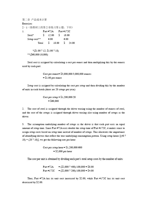
第二章产品成本计算Exercises2–1（指教材上的第2章练习第1题，下同）1. Part #72A Part #172CSteel* $ 12.00 $ 18.00Setup cost** 6.00 6.00Total $ 18.00 $ 24.00*($1.00 ? 12; $1.00 ? 18)**($60,000/10,000)Steel cost is assigned by calculating a cost per ounce and then multiplying this by the ounces used by each part:Cost per ounce= $3,000,000/3,000,000 ounces= $1.00 per ounceSetup cost is assigned by calculating the cost per setup and then dividing this by the number of units in each batch (there are 20 setups per year):Cost per setup = $1,200,000/20= $60,0002. The cost of steel is assigned through the driver tracing using the number of ounces of steel, and the cost of the setups is assigned through driver tracing also using number of setups as the driver.3. The assumption underlying number of setups as the driver is that each part uses an equal amount of setup time. Since Part #72A uses double the setup time of Part #172C, it makes sense to assign setup costs based on setup time instead of number of setups. This illustrates the importance of identifying drivers that reflect the true underlying consumption pattern. Using setup hours [(40 ?10) + (20 ? 10)], we get the following rate per hour:Cost per setup hour = $1,200,000/600= $2,000 per hourThe cost per unit is obtained by dividing each part’s total setup costs by the number of units:Part #72A = ($2,000 ? 400)/100,000 = $8.00Part #172C = ($2,000 ? 200)/100,000 = $4.00Thus, Part #72A has its unit cost increased by $2.00, while Part #172C has its unit cost decreased by $2.00.problems2–51. Nursing hours required per year: 4 ? 24 hours ? 364 days* = 34,944*Note: 364 days = 7 days ? 52 weeksNumber of nurses = 34,944 hrs./2,000 hrs. per nurse = 17.472Annual nursing cost = (17 ? $45,000) + $22,500= $787,500Cost per patient day = $787,500/10,000 days= $78.75 per day (for either type of patient)2. Nursing hours act as the driver. If intensive care uses half of the hours and normal care the other half, then 50 percent of the cost is assigned to each patient category. Thus, the cost per patient day by patient category is as follows:Intensive care = $393,750*/2,000 days= $196.88 per dayNormal care = $393,750/8,000 days= $49.22 per day*$525,000/2 = $262,500The cost assignment reflects the actual usage of the nursing resource and, thus, should be more accurate. Patient days would be accurate only if intensive care patients used the same nursing hours per day as normal care patients.3. The salary of the nurse assigned only to intensive care is a directly traceable cost. To assign the other nursing costs, the hours of additional usage would need to be measured. Thus, both direct tracing and driver tracing would be used to assign nursing costs for this new setting.2–61. Bella Obra CompanyStatement of Cost of Services SoldFor the Year Ended June 30, 2006Direct materials:Beginning inventory $ 300,000Add: Purchases 600,000Materials available $ 900,000Less: Ending inventory 450,000*Direct materials used $ 450,000Direct labor 12,000,000Overhead 1,500,000Total service costs added $ 13,950,000Add: Beginning work in process 900,000Total production costs $ 14,850,000Less: Ending work in process 1,500,000Cost of services sold $ 13,350,000*Materials available less materials used2. The dominant cost is direct labor (presumably the salaries of the 100 professionals). Although labor is the major cost of providing many services, it is not always the case. For example, the dominant cost for some medical services may be overhead (e.g., CAT scans). In some services, the dominant cost may be materials (e.g., funeral services).3. Bella Obra CompanyIncome StatementFor the Year Ended June 30, 2006Sales $ 21,000,000Cost of services sold 13,350,000Gross margin $ 7,650,000Less operating expenses:Selling expenses $ 900,000Administrative expenses 750,000 1,650,000Income before income taxes $ 6,000,0004. Services have four attributes that are not possessed by tangible products: (1) intangibility, (2) perishability, (3) inseparability, and (4) heterogeneity. Intangibility means that the buyers of services cannot see, feel, hear, or taste a service before it is bought. Perishability means that services cannot be stored. This property affects the computation in Requirement 1. Inability to store services means that there will never be any finished goods inventories, thus making the cost of services produced equivalent to cost of services sold. Inseparability simply means that providers and buyers of services must be in direct contact for an exchange to take place. Heterogeneity refers to the greater chance for variation in the performance of services than in the production of tangible products.2–71. Direct materials:Magazine (5,000 ? $0.40) $ 2,000Brochure (10,000 ? $0.08) 800 $ 2,800Direct labor:Magazine [(5,000/20) ? $10] $ 2,500Brochure [(10,000/100) ? $10] 1,000 3,500Manufacturing overhead:Rent $ 1,400Depreciation [($40,000/20,000) ? 350*] 700Setups 600Insurance 140Power 350 3,190Cost of goods manufactured $ 9,490*Production is 20 units per printing hour for magazines and 100 units per printing hour for brochures, yielding monthly machine hours of 350 [(5,000/20) + (10,000/100)]. This is also monthly labor hours, as machine labor only operates the presses.2. Direct materials $ 2,800Direct labor 3,500Total prime costs $ 6,300Magazine:Direct materials $ 2,000Direct labor 2,500Total prime costs $ 4,500Brochure:Direct materials $ 800Direct labor 1,000Total prime costs $ 1,800Direct tracing was used to assign prime costs to the two products.3. Total monthly conversion cost:Direct labor $ 3,500Overhead 3,190Total $ 6,690Magazine:Direct labor $ 2,500Overhead:Power ($1 ? 250) $ 250Depreciation ($2 ? 250) 500Setups (2/3 ? $600) 400Rent and insurance ($4.40 ? 250 DLH)* 1,100 2,250Total $ 4,750Brochure:Direct labor $ 1,000Overhead:Power ($1 ? 100) $ 100Depreciation ($2 ? 100) 200Setups (1/3 ? $600) 200Rent and insurance ($4.40 ? 100 DLH)* 440 940Total $ 1,940*Rent and insurance cannot be traced to each product so the costs are assigned using direct labor hours: $1,540/350 DLH = $4.40 per direct labor hour. The other overhead costs are traced according to their usage. Depreciation and power are assigned by using machine hours (250 for magazines and 100 for brochures): $350/350 = $1.00 per machine hour for power and $40,000/20,000 = $2.00 per machine hour for depreciation. Setups are assigned according to the time required. Since magazines use twice as much time, they receive twice the cost: Letting X = the pro?portion of setup time used for brochures, 2X + X = 1 implies a cost assignment ratio of 2/3 for magazines and 1/3 for brochures.Exercises3–11. Resource Total Cost Unit CostPlastic1 $ 10,800 $0.027Direct labor andvariable overhead2 8,000 0.020Mold sets3 20,000 0.050Other facility costs4 10,000 0.025Total $ 48,800 $0.12210.90 ? $0.03 ? 400,000 = $10,800; $10,800/400,000 = $0.0272$0.02 ? 400,000 = $8,000; $8,000/400,000 = $0.023$5,000 ? 4 quarters = $20,000; $20,000/400,000 = $0.054$10,000; $10,000/400,000 = $0.0252. Plastic, direct labor, and variable overhead are flexible resources; molds and other facility costs are committed resources. The cost of plastic, direct labor, and variable overhead are strictly variable. The cost of the molds is fixed for the particular action figure being produced; it is a step cost for the production of action figures in general. Other facility costs are strictly fixed.3–3High (1,400, $7,950); Low (700, $5,150)V = ($7,950 – $5,150)/(1,400 – 700)= $2,800/700 = $4 per oil changeF = $5,150 – $4(700)= $5,150 – $2,800 = $2,350Cost = $2,350 + $4 (oil changes)Predicted cost for January = $2,350 + $4(1,000) = $6,350problems3–61. High (1,700, $21,000); Low (700, $15,000)V = (Y2 – Y1)/(X2 – X1)= ($21,000 – $15,000)/(1,700 – 700) = $6 per receiving orderF = Y2 – VX2= $21,000 – ($6)(1,700) = $10,800Y = $10,800 + $6X2. Output of spreadsheet regression routine with number of receiving orders as the independent variable:Constant 4512.98701298698Std. Err. of Y Est. 3456.24317476605R Squared 0.633710482694768No. of Observations 10Degrees of Freedom 8X Coefficient(s) 13.3766233766234Std. Err. of Coef. 3.59557461331427V = $13.38 per receiving order (rounded)F = $4,513 (rounded)Y = $4,513 + $13.38XR2 = 0.634, or 63.4%Receiving orders explain about 63.4 percent of the variability in receiving cost, providing evidence that Tracy’s choice o f a cost driver is reasonable. However, other drivers may need to be considered because 63.4 percent may not be strong enough to justify the use of only receiving orders.3. Regression with pounds of material as the independent variable:Constant 5632.28109733183Std. Err. of Y Est. 2390.10628259277R Squared 0.824833789433823No. of Observations 10Degrees of Freedom 8X Coefficient(s) 0.0449642991356633Std. Err. of Coef. 0.0073259640055344V = $0.045 per pound of material delivered (rounded)F = $5,632 (rounded)Y = $5,632 + $0.045XR2 = 0.825, or 82.5%Pounds of material delivered explains about 82.5 percent of the variability in receiving cost. This is a better result than that of the receiving orders and should convince Tracy to try multiple regression.4. Regression routine with pounds of material and number of receiving orders as the independent variables:Constant 752.104072925631Std. Err. of Y Est. 1350.46286973443R Squared 0.951068418023306No. of Observations 10Degrees of Freedom 7X Coefficient(s) 0.0333883151096915 7.14702865269395Std. Err. of Coef. 0.00495524841198368 1.68182916088492V1 = $0.033 per pound of material delivered (rounded)V2 = $7.147 per receiving order (rounded)F = $752 (rounded)Y = $752 + $0.033a + $7.147bR2 = 0.95, or 95%Multiple regression with both variables explains 95 percent of the variability in receiving cost. This is the best result.5–21. Job #57 Job #58 Job #59Balance, 7/1 $ 22,450 $ 0 $ 0Direct materials 12,900 9,900 35,350Direct labor 20,000 6,500 13,000Applied overhead:Power 750 600 3,600Material handling 1,500 300 6,000Purchasing 250 1,000 250Total cost $ 57,850 $ 18,300 $ 58,2002. Ending balance in Work in Process = Job #58 = $18,3003. Ending balance in Finished Goods = Job #59 = $58,2004. Cost of Goods Sold = Job #57 = $57,850problems5–31. Overhead rate = $180/$900 = 0.20 or 20% of direct labor dollars.(This rate was calculated using information from the Ladan job; however, the Myron and Coe jobs would give the same answer.)2. Ladan Myron Coe Walker WillisBeginning WIP $ 1,730 $1,180 $2,500 $ 0 $ 0Direct materials 400 150 260 800 760Direct labor 800 900 650 350 900Applied overhead 160 180 130 70 180Total $ 3,090 $2,410 $3,540 $ 1,220 $ 1,840Note: This is just one way of setting up the job-order cost sheets. You might prefer to keep the detail on the materials, labor, and overhead in beginning inventory costs.3. Since the Ladan and Myron jobs were completed, the others must still be in process. Therefore, the ending balance in Work in Process is the sum of the costs of the Coe, Walker, and Willis jobs.Coe $3,540Walker 1,220Willis 1,840Ending Work in Process $6,600Cost of Goods Sold = Ladan job + Myron job = $3,090 + $2,410 = $5,5004. Naman CompanyIncome StatementFor the Month Ended June 30, 20XXSales (1.5 ? $5,500) $8,250Cost of goods sold 5,500Gross margin $2,750Marketing and administrative expenses 1,200Operating income $1,5505–201. Overhead rate = $470,000/50,000 = $9.40 per MHr2. Department A: $250,000/40,000 = $6.25 per MHrDepartment B: $220,000/10,000 = $22.00 per MHr3. Job #73 Job #74Plantwide:70 ? $9.40 = $658 70 ? $9.40 = $658Departmental:20 ? $6.25 $ 125.00 50 ? $6.25 $ 312.5050 ? $22 1,100.00 20 ? $22 440.00$ 1,225.00 $ 752.50Department B appears to be more overhead intensive, so jobs spending more time in Department B ought to receive more overhead. Thus, departmental rates provide more accuracy.4. Plantwide rate: $250,000/40,000 = $6.25Department B: $62,500/10,000 = $6.25Job #73 Job #74Plantwide:70 ? $6.25 = $437.50 70 ? $6.25 = $437.50Departmental:20 ? $6.25 $ 125.00 50 ? $6.25 $ 312.5050 ? $6.25 312.50 20 ? $6.25 125.00$ 437.50 $ 437.50Assuming that machine hours is a good cost driver, the departmental rates reveal that overhead consumption is the same in each department. In this case, there is no need for departmental rates, and a plantwide rate is sufficient.5–41. Overhead rate = $470,000/50,000 = $9.40 per MHr2. Department A: $250,000/40,000 = $6.25 per MHrDepartment B: $220,000/10,000 = $22.00 per MHr3. Job #73 Job #74Plantwide:70 ? $9.40 = $658 70 ? $9.40 = $658Departmental:20 ? $6.25 $ 125.00 50 ? $6.25 $ 312.5050 ? $22 1,100.00 20 ? $22 440.00$ 1,225.00 $ 752.50Department B appears to be more overhead intensive, so jobs spending more time in Department B ought to receive more overhead. Thus, departmental rates provide more accuracy.4. Plantwide rate: $250,000/40,000 = $6.25Department B: $62,500/10,000 = $6.25Job #73 Job #74Plantwide:70 ? $6.25 = $437.50 70 ? $6.25 = $437.50Departmental:20 ? $6.25 $ 125.00 50 ? $6.25 $ 312.5050 ? $6.25 312.50 20 ? $6.25 125.00$ 437.50 $ 437.50Assuming that machine hours is a good cost driver, the departmental rates reveal that overhead consumption is the same in each department. In this case, there is no need for departmental rates, and a plantwide rate is sufficient.5–51. Last year’s unit-based overhead rate = $50,000/10,000 = $5This year’s unit-based overhead rate = $100,000/10,000 = $10Last Year This YearBike cost:2 ? $20 $ 40 $ 403 ? $12 36 36Overhead:5 ? $5 255 ? $10 50Total $101 $126Price last year = $101 ? 1.40 = $141.40/dayPrice this year = $126 ? 1.40 = $176.40/dayThis is a $35 increase over last year, nearly a 25 percent increase. No doubt the Carsons arenot pleased and would consider looking around for other recreational possibilities.2. Purchasing rate = $30,000/10,000 = $3 per purchase orderPower rate = $20,000/50,000 = $0.40 per kilowatt hourMaintenance rate = $6,000/600 = $10 per maintenance hourOther rate = $44,000/22,000 = $2 per DLHBike Rental Picnic CateringPurchasing$3 ? 7,000 $21,000$3 ? 3,000 $ 9,000Power$0.40 ? 5,000 2,000$0.40 ? 45,000 18,000Maintenance$10 ? 500 5,000$10 ? 100 1,000Other$2 ? 11,000 22,000 22,000Total overhead $50,000 $50,0003. This year’s bike rental overhead rate = $50,000/10,000 = $5Carson rental cost = (2 ? $20) + (3 ? $12) + (5 ? $5) = $101Price = 1.4 ? $101 = $141.40/day4. Catering rate = $50,000/11,000 = $4.55* per DLHCost of Estes job:Bike rental rate (2 ? $7.50) $15.00Bike conversion cost (2 ? $5.00) 10.00Catering materials 12.00Catering conversion (1 ? $4.55) 4.55Total cost $41.55*Rounded5. The use of ABC gives Mountain View Rentals a better idea of the types and costs of activities that are used in their business. Adding Level 4 bikes will increase the use of the most expensive activities, meaning that the rental rate will no longer be an average of $5 per rental day. Mountain View Rentals might need to set a Level 4 price based on the increased cost of both the bike and conversion cost.分步成本法6–11. Cutting Sewing PackagingDepartment Department DepartmentDirect materials $5,400 $ 900 $ 225Direct labor 150 1,800 900Applied overhead 750 3,600 900Transferred-in cost:From cutting 6,300From sewing 12,600Total manufacturing cost $6,300 $12,600 $14,6252. a. Work in Process—Sewing 6,300Work in Process—Cutting 6,300b. Work in Process—Packaging 12,600Work in Process—Sewing 12,600c. Finished Goods 14,625Work in Process—Packaging 14,625 3. Unit cost = $14,625/600 = $24.38* per pair6–21. Units transferred out: 27,000 + 33,000 – 16,200 = 43,8002. Units started and completed: 43,800 – 27,000 = 16,8003. Physical flow schedule:Units in beginning work in process 27,000Units started during the period 33,000Total units to account for 60,000Units started and completed 16,800Units completed from beginning work in process 27,000Units in ending work in process 16,200Total units accounted for 60,0004. Equivalent units of production:Materials ConversionUnits completed 43,800 43,800Add: Units in ending work in process:(16,200 ? 100%) 16,200(16,200 ? 25%) 4,050 Equivalent units of output 60,000 47,8506–31. Physical flow schedule:Units to account for:Units in beginning work in process 80,000Units started during the period 160,000Total units to account for 240,000Units accounted for:Units completed and transferred out:Started and completed 120,000From beginning work in process 80,000 200,000 Units in ending work in process 40,000Total units accounted for 240,0002. Units completed 200,000Add: Units in ending WIP ? Fraction complete(40,000 ? 20%) 8,000Equivalent units of output 208,0003. Unit cost = ($374,400 + $1,258,400)/208,000 = $7.854. Cost transferred out = 200,000 ? $7.85 = $1,570,000Cost of ending WIP = 8,000 ? $7.85 = $62,8005. Costs to account for:Beginning work in process $ 374,400Incurred during June 1,258,400Total costs to account for $ 1,632,800Costs accounted for:Goods transferred out $ 1,570,000Goods in ending work in process 62,800Total costs accounted for $ 1,632,8006–31、Units t0 account for:Units in beginning work in process(25% completed) 10000Units started during the period 70000 Total units to account for 80000 Units accounted forUnits completed and transferred outStarted and completed 50000From beginning work in process 10000 60000 Units in ending work in process(60% completed) 20000 Total units accounted for 80000 2、60000+20000×60%=72000（units）3、Unit cost for materials:（$/unit）Unit cost for convension:（$/unit）Total unit cost:5+1.13=6.13（$/unit）4、The cost of units of transferred out:60000×6.13=367800($)The cost of units of ending work in process:20000×5+20000×20%×1.13=113560($)作业成本法4–21. Predetermined rates:Drilling Department: Rate = $600,000/280,000 = $2.14* per MHrAssembly Department: Rate = $392,000/200,000= $1.96 per DLH*Rounded2. Applied overhead:Drilling Department: $2.14 ? 288,000 = $616,320Assembly Department: $1.96 ? 196,000 = $384,160Overhead variances:Drilling Assembly TotalActual overhead $602,000 $ 412,000 $ 1,014,000Applied overhead 616,320 384,160 1,000,480Overhead variance $ (14,320) over $ 27,840 under $ 13,5203. Unit overhead cost = [($2.14 ? 4,000) + ($1.96 ? 1,600)]/8,000= $11,696/8,000= $1.46**Rounded4–31. Yes. Since direct materials and direct labor are directly traceable to each product, their cost assignment should be accurate.2. Elegant: (1.75 ? $9,000)/3,000 = $5.25 per briefcaseFina: (1.75 ? $3,000)/3,000 = $1.75 per briefcaseNote: Overhead rate = $21,000/$12,000 = $1.75 per direct labor dollar (or 175 percent of direct labor cost).There are more machine and setup costs assigned to Elegant than Fina. This is clearly a distortion because the production of Fina is automated and uses the machine resources much more than the handcrafted Elegant. In fact, the consumption ratio for machining is 0.10 and 0.90 (using machine hours as the measure of usage). Thus, Fina uses nine times the machining resources as Elegant. Setup costs are similarly distorted. The products use an equal number of setups hours. Yet, if direct labor dollars are used, then the Elegant briefcase receives three times more machining costs than the Fina briefcase.3. Overhead rate = $21,000/5,000= $4.20 per MHrElegant: ($4.20 ? 500)/3,000 = $0.70 per briefcaseFina: ($4.20 ? 4,500)/3,000 = $6.30 per briefcaseThis cost assignment appears more reasonable given the relative demands each product places on machine resources. However, once a firm moves to a multiproduct setting, using only one activity driver to assign costs will likely produce product cost distortions. Products tend to make different demands on overhead activities, and this should be reflected in overhead cost assignments. Usually, this means the use of both unit- and nonunit-level activity drivers. In this example, there is a unit-level activity (machining) and a nonunit-level activity (setting up equipment). The consumption ratios for each (using machine hours and setup hours as the activity drivers) are as follows:Elegant FinaMachining 0.10 0.90 (500/5,000 and 4,500/5,000)Setups 0.50 0.50 (100/200 and 100/200)Setup costs are not assigned accurately. Two activity rates are needed—one based on machine hours and the other on setup hours:Machine rate: $18,000/5,000 = $3.60 per MHrSetup rate: $3,000/200 = $15 per setup hourCosts assigned to each product:Machining: Elegant Fina$3.60 ? 500 $ 1,800$3.60 ? 4,500 $ 16,200Setups:$15 ? 100 1,500 1,500Total $ 3,300 $ 17,700Units ÷3,000 ÷3,000Unit overhead cost $ 1.10 $ 5.904：Elegant Unit overhead cost：[9000+3000+18000*500/5000+3000/2]/3000=$5.1 Fina Unit overhead cost：[3000+3000+18000*4500/5000+3000/2]/3000=$7.94–51. Deluxe Percent Regular PercentPrice $900 100% $750 100%Cost 576 64 600 80Unit gross profit $324 36% $150 20%Total gross profit:($324 ? 100,000) $32,400,000($150 ? 800,000) $120,000,0002. Calculation of unit overhead costs:Deluxe gularUnit-level:Machining:$200 ? 100,000 $20,000,000$200 ? 300,000 $60,000,000Batch-level:Setups:$3,000 ? 300 900,000$3,000 ? 200 600,000Packing:$20 ? 100,000 2,000,000$20 ? 400,000 8,000,000Product-level:Engineering:$40 ? 50,000 2,000,000$40 ? 100,000 4,000,000Facility-level:Providing space:$1 ? 200,000 200,000$1 ? 800,000 800,000Total overhead $25,100,000 $73,400,000Units ÷100,000 ÷800,000Overhead per unit $251 $91.75Deluxe Percent Regular PercentPrice $900 100% $750.00 100%Cost 780* 87*** 574.50** 77***Unit gross profit $120 13%*** $175.50 23%***Total gross profit:($120 ? 100,000) $12,000,000($175.50 ? 800,000) $140,400,000*$529 + $251**$482.75 + $91.753. Using activity-based costing, a much different picture of the deluxe and regular products emerges. The regular model appears to be more profitable. Perhaps it should be emphasized.4–61. JIT Non-JITSalesa $12,500,000 $12,500,000Allocationb 750,000 750,000a$125 ? 100,000, where $125 = $100 + ($100 ? 0.25), and 100,000 is the average order size times the number of ordersb0.50 ? $1,500,0002. Activity rates:Ordering rate = $880,000/220 = $4,000 per sales orderSelling rate = $320,000/40 = $8,000 per sales callService rate = $300,000/150 = $2,000 per service callJIT Non-JITOrdering costs:$4,000 ? 200 $ 800,000$4,000 ? 20 $ 80,000Selling costs:$8,000 ? 20 160,000$8,000 ? 20 160,000Service costs:$2,000 ? 100 200,000$2,000 ? 50 100,000Total $1,160,000 $340,0 0For the non-JIT customers, the customer costs amount to $750,000/20 = $37,500 per order under the original allocation. Using activity assign?ments, this drops to $340,000/20 = $17,000 per order, a difference of $20,500 per order. For an order of 5,000 units, the order price can be decreased by $4.10 per unit without affecting customer profitability. Overall profitability will decrease, however, unless the price for orders is increased to JIT customers.3. It sounds like the JIT buyers are switching their inventory carrying costs to Emery without any significant benefit to Emery. Emery needs to increase prices to reflect the additional demands on customer-support activities. Furthermore, additional price increases may be needed to reflectthe increased number of setups, purchases, and so on, that are likely occurring inside the plant. Emery should also immediately initiate discussions with its JIT customers to begin negotiations for achieving some of the benefits that a JIT supplier should have, such as long-term contracts. The benefits of long-term contracting may offset most or all of the increased costs from the additional demands made on other activities.4–71. Supplier cost:First, calculate the activity rates for assigning costs to suppliers:Inspecting components: $240,000/2,000 = $120 per sampling hourReworking products: $760,500/1,500 = $507 per rework hourWarranty work: $4,800/8,000 = $600 per warranty hourNext, calculate the cost per component by supplier:Supplier cost:Vance FoyPurchase cost:$23.50 ? 400,000 $ 9,400,000$21.50 ? 1,600,000 $ 34,400,000Inspecting components:$120 ? 40 4,800$120 ? 1,960 235,200Reworking products:$507 ? 90 45,630$507 ? 1,410 714,870Warranty work:$600 ? 400 240,000$600 ? 7,600 4,560,000Total supplier cost $ 9,690,430 $ 39,910,070Units supplied ÷400,000 ÷1,600,000Unit cost $ 24.23* $ 24.94**RoundedThe difference is in favor of Vance; however, when the price concession is considered, the cost of Vance is $23.23, which is less than Foy’s component. Lumus should accept the contractual offer made by Vance.4–7 Concluded2. Warranty hours would act as the best driver of the three choices. Using this driver, the rate is $1,000,000/8,000 = $125 per warranty hour. The cost assigned to each component would be:Vance FoyLost sales:$125 ? 400 $ 50,000$125 ? 7,600 $ 950,000$ 50,000 $ 950,000Units supplied ÷400,000 ÷1,600,000Increase in unit cost $ 0.13* $ 0.59**Rounded$0.075 per unitCategory II: $45/1,000 = $0.045 per unitCategory III: $45/1,500 = $0.03 per unitCategory I, which has the smallest batches, is the most undercosted of the three categories. Furthermore, the unit ordering cost is quite high relative to Category I’s selling price (9 to 15 percent of the selling price). This suggests that something should be done to reduce the order-filling costs.3. With the pricing incentive feature, the average order size has been increased to 2,000 units for all three product families. The number of orders now processed can be calculated as follows:Orders = [(600 ? 50,000) + (1,000 ? 30,000) + (1,500 ? 20,000)]/2,000= 45,000Reduction in orders = 100,000 – 45,000 = 55,000Steps that can be reduced = 55,000/2,000 = 27 (rounding down to nearest whole number)There were initially 50 steps: 100,000/2,000Reduction in resource spending:Step-fixed costs: $50,000 ? 27 = $1,350,000Variable activity costs: $20 ? 55,000 = 1,100,000$2,450,000预算9-4Norton, Inc.Sales Budget For the Coming YearModel Units Price Total SalesLB-1 50,400 $29.00 $1,461,600LB-2 19,800 15.00 297,000WE-6 25,200 10.40 262,080 WE-7 17,820 10.00 178,200 WE-8 9,600 22.00 211,200 WE-9 4,000 26.00 104,000 Total $2,514,080二、1. Raylene’s Flowers and GiftsProduction Budget for Gift BasketsFor September, October, November, and DecemberSept. Oct. Nov. D ec.Sales 200 150 180 250Desired ending inventory 15 18 25 10Total needs 215 168 205 260Less: Beginning inventory 20 15 18 25 Units produced 195 153 187 2352. Raylene’s Flowers and GiftsDirect Materials Purchases BudgetFor September, October, and NovemberFruit: Sept. Oct. Nov.Production 195 153 187? Amount/basket (lbs.) ? 1 ? 1 ?1Needed for production 195 153 187Desired ending inventory 8 9 12Needed 203 162 200Less: Beginning inventory 10 8 9Purchases193 154 190Small gifts: Sept. Oct. Nov.Production 195 153 187 ? Amount/basket (items) ? 5 ? 5 ? 5Needed for production 975 765 935Desired ending inventory 383 468 588Needed 1,358 1,233 1,523Less: Beginning inventory 488 383 468Purchases 870 850 1,055Cellophane: Sept. Oct. Nov.Production 195 153 187。

中级财务会计(双语)第四章

Inventory category Ⅰ Item A Item B Inventory category Ⅱ Item C Item D Item E
Applying LCM method
• Use LCM to determine the inventory value. Three applications:
150,000
80,000 90,000 95,000 265,000 415,000
155,000
65,000 56,000 86,000 207,000
150,000
207,000 357,000
Adjusting Cost to Market
• • • Write-down of inventory =415,000-357,000=58,000 Dr. Loss on write-down of inventory 58,000 Cr. Inventory valuation allowance 58,000
Impairment of Inventories
• How do we know we have an impairment of inventories? 如何判断存货存在减值迹象？ • Impairment is incurred:
▪ If those inventories are damaged 被损坏 ▪ If inventories have become wholly or partially obsolete 部分或全部过时 ▪ If their selling prices have declined 市价下跌 ▪ If the estimated costs of completion or the estimated costs to be incurred to make the sale have increased. 估计的完工成本或估计的销售费用上涨

公司亏损怎么补救英语作文

公司亏损怎么补救英语作文下载温馨提示:该文档是我店铺精心编制而成，希望大家下载以后，能够帮助大家解决实际的问题。

文档下载后可定制随意修改，请根据实际需要进行相应的调整和使用，谢谢!并且，本店铺为大家提供各种各样类型的实用资料，如教育随笔、日记赏析、句子摘抄、古诗大全、经典美文、话题作文、工作总结、词语解析、文案摘录、其他资料等等，如想了解不同资料格式和写法，敬请关注!Download tips: This document is carefully compiled by theeditor. I hope that after you download them,they can help yousolve practical problems. The document can be customized andmodified after downloading,please adjust and use it according toactual needs, thank you!In addition, our shop provides you with various types ofpractical materials,such as educational essays, diaryappreciation,sentence excerpts,ancient poems,classic articles,topic composition,work summary,word parsing,copyexcerpts,other materials and so on,want to know different data formats andwriting methods,please pay attention!One possible way to remedy a company's loss is by cutting costs. This can be achieved by reducing unnecessary expenses, such as office supplies, travel expenses, and employee benefits. Additionally, the company can consider downsizing its workforce or renegotiating contracts with suppliers to obtain better deals. By implementing these cost-cutting measures, the company can potentially save money and improve its financial situation.Another strategy to recover from a loss is to increase revenue. This can be done by expanding the customer base through marketing and advertising efforts. The company can also consider launching new products or services to attract more customers. Additionally, the company can explore partnerships or collaborations with other businesses to tap into new markets or offer complementary products. By generating more sales and revenue, the company can offset its losses and regain financial stability.Furthermore, improving efficiency and productivity within the company can also help mitigate losses. This can be achieved by implementing streamlined processes and utilizing technology to automate tasks. The company can also invest in employee training and development to enhance their skills and productivity. By improving efficiency, the company can reduce costs and maximize its resources, ultimately improving its financial performance.In addition to these measures, seeking financial assistance or investment can also be considered as a way to remedy a company's loss. This can be done by approaching banks or financial institutions for loans or exploring options for equity investment. By injecting additional capital into the company, it can have the necessary funds to overcome its losses and support its operations.Lastly, it is important for the company to continuously monitor and analyze its financial performance. By regularly reviewing financial statements and conducting thorough analysis, the company can identify areas of improvement and take necessary actions promptly. This can involve adjustingstrategies, reallocating resources, or making changes tothe business model. By staying proactive and responsive to the financial situation, the company can increase its chances of recovering from a loss.Overall, there are various approaches that can be taken to remedy a company's loss. By cutting costs, increasing revenue, improving efficiency, seeking financial assistance, and monitoring financial performance, the company can work towards overcoming its losses and achieving financial stability.。

1、下载文档前请自行甄别文档内容的完整性，平台不提供额外的编辑、内容补充、找答案等附加服务。
2、"仅部分预览"的文档,不可在线预览部分如存在完整性等问题,可反馈申请退款(可完整预览的文档不适用该条件!)。
3、如文档侵犯您的权益，请联系客服反馈,我们会尽快为您处理(人工客服工作时间：9:00-18:30)。

Considering lost sale in inventory routing problems for perishable goodsqSamira Mirzaei a ,Abbas Seiﬁb ,⇑a Cluster for Operations Research and Logistics,Department of Economics and Business,Aarhus University,Aarhus,Denmark bDepartment of Industrial Engineering and Management Systems,Amirkabir University of Technology,Tehran,Irana r t i c l e i n f o Article history:Received 15December 2012Received in revised form 22April 2015Accepted 6May 2015Available online 14May 2015Keywords:Inventory routing problem Perishable goods Lost saleSimulated annealing Tabu searcha b s t r a c tThis paper presents a mathematical model for an inventory routing problem (IRP).The model is especially designed for allocating the stock of perishable goods.It is assumed that the age of the perishable inven-tory has a negative impact on the demand of end customers and a percentage of the demand is consid-ered as lost sale.The proposed model balances the transportation cost,the cost of inventory holding and lost sale.In addition to the usual inventory routing constraints,we consider the cost of lost sale as a linear or an exponential function of the inventory age.The proposed model is solved to optimality for small instances and is used to obtain lower bounds for larger instances.We have also devised an efﬁcient meta-heuristic algorithm to ﬁnd good solutions for this class of problems based on Simulated Annealing (SA)and Tabu Search (TS).Computational results indicate that,for small problems,the average optimality gaps are less than 10.9%and 13.4%using linear and exponential lost sale functions,respec-tively.Furthermore,we show that the optimality gaps found by CPLEX grow exponentially with the prob-lem size while those obtained by the proposed meta-heuristic algorithm increase linearly.Ó2015Elsevier Ltd.All rights reserved.1.IntroductionInventory routing problem (IRP)is a major concern in supply chain management.The aim is to integrate the transportation activities and inventory management along the supply chain and avoid the inefﬁciency caused by solving the underlying vehicle routing and inventory subproblems separately.Recent studies assume that an indeﬁnite number of stock items can be stored to meet future customers’demand.However,the impact of perishability cannot be ignored for certain types of goods that deteriorate over time and may become partially or entirely unsuitable for consumption (Shen,Dessouky,&Ordonez,2011).Deteriorating items refer to items that get damaged,spoiled,dried,invalid,or degraded over time (Li,Lan,&Mawhinney,2010)and can be classiﬁed into two groups:perishable products and decay-ing products.Items such as meat,green vegetables,human blood,medicine,ﬂowers,and ﬁlms that have a maximum usable lifetime are known as perishable modities like alcohol andgasoline that have no shelf-life are known as decaying products (Goyal &Giri,2001).Although the life of the perishable products can be prolonged by advanced cooling equipment,these products lose their quality over time and this will cause a decrease in the demand for these products.If perishable products are not delivered to retailers on a daily basis,due to the limited lifetime and possible degradation of these products,some customers will refrain from purchasing them.Thus,the demand for the products is affected by the age of the perishable inventory.In IRP literature,some models consider shortage,stock out,or backorder costs (see for instance:Abdelmaguid &Dessouky,2006;Abdelmaguid,Dessouky,&Ordóñez,2009;Herer &Roundy,1997;Jaillet,Bard,Huang,&Dror,2002).Modeling IRP with deteriorating products and the associated cost of lost sale has not been explicitly considered in the literature.In this paper,we speciﬁcally calculate the cost of lost sale in the supply chain for perishable goods to avoid overstocking such items in an attempt to reduce transportation cost.This paper formulates a multi-period inventory routing prob-lem for perishable goods in which the end customers’demand depends on the age of the inventory.The proposed model includes vehicle routing decisions as well as delivery and inventory deci-sions over a speciﬁc planning horizon.It is a non-linear mixed/10.1016/j.cie.2015.05.0100360-8352/Ó2015Elsevier Ltd.All rights reserved.qThis manuscript was processed by Area Editor I-Lin Wang.⇑Corresponding author at:Department of Industrial Engineering and Manage-ment Systems,Amirkabir University of Technology (Tehran Polytechnic),P.O.Box 15875-4413,Tehran,Iran.Tel.:+9864545377;fax:+9866954569.E-mail address:aseiﬁ@aut.ac.ir (A.Seiﬁ).integer programming model which is linearized to be solvable efﬁ-ciently.The objective function is to minimize the total cost of transportation,lost sale,and holding inventories.In addition to the usual inventory routing constraints,we consider a nonlinear constraint that deﬁnes the inventory age as a function of delivery date.The lost sale is assumed to be a linear or an exponential func-tion of the inventory age.The mathematical model with both linear and exponential lost sale functions is solved up to optimality for small to medium size problems.It is also used toﬁnd some lower bounds for larger instances.Since such problems are NP-hard due to the underlying vehicle routing problem(VRP),we develop a heuristic algorithm within a metaheuristic framework for solving larger problem instances.The rest of this paper is organized as follows.Section2reviews the literature on inventory management and vehicle routing prob-lems for perishable goods.In Section3,the problem is formulated as a mathematical model using two different lost sale functions. The metaheuristic algorithm is described in Section4,followed by the results of computational experiments in Section5. Conclusions and some directions for future research are described in Section6.2.Literature reviewIn this section,we review the literature related to inventory management and vehicle routing problems with regards to perish-able goods.Due to the importance of assumption on retailers’orders in modeling the inventory of perishable goods,researchers have studied a variety of constant demand,time-varying demand, stock dependent and price dependent demand(see Goyal&Giri, 2001;Li et al.,2010;Raafat,1991;Shah&Shah,2000).Many researchers have developed inventory models for deteriorating items with time varying end customer demand using linearly or exponentially decreasing demand(see,for instance:Chung& Ting,1993;Dave&Patel,1981;Giri&Chaudhuri,1997;Hariga& Benkherouf,1994;Sachan,1984;Wee,1995;Xu&Wang,2003). This paper also assumes that the demand of end customers is a lin-early or an exponentially decreasing function of the age of perish-able goods.Tarantilis and Kiranoudis(2001)proposed a threshold-accepting algorithm to solve a fresh milk distribution problem for a dairy company in Greece.They focused on a routing problem using heterogeneous vehicles.Tarantilis and Kiranoudis (2002)solved the distribution of fresh meat products in Greece using an open multi-depot VRP.They did not consider any addi-tional constraints reﬂecting the perishable nature of those com-modities.Hsu,Hung,and Li(2007)developed a stochastic VRP model to obtain optimal delivery routes,loads,ﬂeet dispatching and departure times for distribution of perishable food.Their objective function was to minimize the cost of dispatching vehicles transportation as well as the inventory,energy and penalty costs for violating the time window constraints.Osvald and Stirn (2008)developed a heuristic algorithm for the problem of dis-tributing fresh vegetables in which the impact of perishability of the goods was considered as a part of the overall distribution cost. However,since additional cost of distribution of perishable goods is insigniﬁcant compared to the transportation cost,we do not con-sider such details in our modeling of the VRP subproblem.This is in agreement with the practical consideration reported by Tarantilis and Kiranoudis(2001)and Tarantilis and Kiranoudis(2002).Federgruen,Prastacos,and Zipkin(1986)are among the pioneering scholars who integrated the routing and inventory allo-cation in a single period problem assuming random retailers’demand for perishable products.They classiﬁed perishable products into old and fresh items.Old items would perish in the present period while other goods would be considered fresh for at least one period before becoming outdated.Le,Diabat,Richard, and Yih(2012)presented a multi-period IRP model for perishable products with aﬁxed shelf life in which the customer demand was deterministic and unsold goods with no value were discarded.A pathﬂow formulation for this problem was proposed and a lower bound for the problem was obtained using column generation.In addition to the regular IRP constraints,they added another con-straint guaranteeing that a retailer should not have an inventory greater than the total demand in the next consecutive time periods based on maximum shelf life of the perishable goods.Furthermore,due to the nature of perishable products,some researchers integrated production planning or facility location problem with the VRP or IRP for perishable products(see Karaesmen,Scheller-Wolf,&Deniz,2011).For example,Chen, Hsueh,and Chang(2009)considered the production schedule and delivery routes decisions simultaneously in order to maximize the expected proﬁt of the supplier.Seyedhosseini and Ghoreyshi (2014)integrated production and distribution planning in an IRP model to determine product quantities,the number of distribution centers to be visited,and the quantities of perishable products to be delivered.Hiassat and Diabat(2011)proposed a model for dete-riorating items in which the inventory location problem was inte-grated with the routing decisions for deterministic demand.We do not,however,take the production program or facility location into consideration in this paper and we focus on IRP for perishable goods.We have not found any literature that includes the cost of lost sale explicitly in the formulation of IRP for perishable goods as considered in our paper.3.Problem deﬁnitionWe consider a two-echelon supply chain involving a depot,a set of retailers,and aﬂeet of capacitated homogenous vehicles.A cen-tral depot(supplier)serves a set of geographically scattered retail-ers having deterministic demand.Perishable items are transported from the depot to the retailers in such a way that out-of-stock sit-uations never occur.The problem is a multi-period routing and inventory planning problem with aﬁnite time horizon.Retailers have limited storage capacities and their demand in each period is assumed to be known and should be met by the end of each per-iod.It is also assumed that the end customer’s demand is a linearly or exponentially decreasing function of the age of the perishable goods and any inventory unsold by the time of the next delivery is considered as lost sale.We propose a mixed integer nonlinear programming model whose objective function is the sum of the transportation cost,and the cost of inventory holding and lost sale. In addition to the usual inventory routing constraints,we consider a nonlinear constraint that deﬁnes the inventory age as a function of the delivery date.The lost sale is then expressed as either a lin-ear or an exponential function of the inventory age.The assump-tions on the VRP subproblem are the same as the ones in the classical models.Each vehicle starts its tour from the central depot and returns to the central depot after delivering the goods to a set of retailers assigned to that vehicle.A retailer is served only once and by one vehicle in each period.3.1.Model formulationIn this section,we develop a mixed integer non-linear program-ming model for the IRP with lost sale(named as IRPLS)and lin-earize it to make it solvable using CPLEX.First,the following sets, constants,parameters,and decision variables are introduced:214S.Mirzaei,A.Seiﬁ/Computers&Industrial Engineering87(2015)213–227Index sets:R:Retailer set.D:Set of central depots.N:Set of all pointsðR[DÞ.T:Set of time periods.K:Vehicle set.Constants and parameters:c ij:Travel cost from retailer/depot i to retailer/depot j for i2N;j2N;satisfying the triangular inequality:c ikþc kj P c ij; 8i;j;k2N.a i:Lost sale cost per period per unit for i2R.h i:Holding cost per period per unit for i2R.d it:Demand of retailer i in period t for t2T;i2R.V i:Storage capacity of retailer i for i2R.S i:Time to serve retailer i for i2R.t ij:Travel time from point i to point j for i;j2N.b i:Initial amount of inventory of retailer i for i2R.b:The rate at which the end customer’s demand is decreasing ð0<b<1Þ.LT:Length of each time period.Q:Vehicle capacity.M:A large positive number.Decision variables:X ijkt¼1;If vehicle k travels from point i to point j in period t; 0;Otherwise:&Y ikt¼1;If vehicle k visits point i in period t; 0;Otherwise:&W ikt:The delivered amount to retailer i by vehicle k in period t;Other variables:I i;t:Inventory amount of retailer i in period t for i2R,t2T.api;t:The age of inventory of retailer i in period t,t2T;i2R.U it:Total amount of goods delivered by a vehicle after visiting retailer i in period t.The objective function is to minimize the following costs:1.transportation,2.holding inventory,and3.lost sale.The cost of lost sale is a function of the inventory ageðapi;tÞand b.We consider two forms of lost sale functions:a linear and an exponential trend.The linear cost function of lost sale is calculated as a iÂd itÂbÂap i;t and the exponential cost function has the form a iÂd itÂð1ÀeÀbÂap i;tÞ.Therefore,the linear objective function of the proposed multi-period IRP model is formulated as:Min z1¼Xi2N Xj2NXk2KXt2Tc ij X ijkt!þXi2RXt2Th i I i;t!þXi2R Xt2Ta iÁd itÁbÁapi;t!ð1ÞSince customers’demand for most perishable goods have an exponential trend,the second objective function with an exponen-tial lost sale is formulated as follows:Min z2¼Xi2NXj2NXk2KXt2Tc ij X ijkt!þXi2RXt2Th i I i;t!þXi2RXt2Ta iÁd i;tÁ1ÀeÀbÁap i;tÀÁ!ð2ÞThe model constraints are given by(3)–(18)as follows:Xi2Ni–jX ijktÀY jkt¼0;8j2N;8k2K;8t2Tð3ÞXj2Ni–jX ijktÀY ikt¼0;8i2N;8k2K;8t2Tð4ÞXk2KY ikt61;8i2R;8t2Tð5ÞXi2RXj2Ni–jS i X ijktþXi2NXj2Ni–jt ij X ijkt6LT;8k2K;8t2Tð6Þapi;t¼ðap i;tÀ1þ1ÞÁ1ÀXk2KY ikt!;8i2R;8t2Tð7ÞI i;tÀ1þXk2KW ikt¼I i;tþd it;8i2R;8t2Tð8ÞI i;t6V i;8i2R;8t2T;8k2Kð9ÞW ikt6QÂY ikt;8i2R;8k2K;8t2Tð10ÞXi2RW ikt6Q;8k2K;8t2Tð11ÞU itÀU jtþQÂX ijkt6QÀD jt;8i;j2R;i–j;8k2K;8t2Tð12ÞD it6U it6Q;8i2R;8t2Tð13ÞX ijkt2f0;1g;8i;j2N;i–j;8k2K;8t2Tð14ÞY ikt2f0;1g;8i2R;8k2K;8t2Tð15ÞW ikt P0;8i2R;8k2K;8t2Tð16ÞI i;t P0;8i2R;8t2Tð17Þapi;t2f0;1;...;TÀ1g;8i2R;8t2Tð18ÞConstraints(3)and(4)deﬁne the assignment of each node to a tour and the ordinaryﬂow conservation at each node.Constraints (5)specify that each retailer is visited at most once every day. Constraints(6)ensure that the total of service times and transit times in each tour assigned to a vehicle does not exceed the length of working hours in each period.This is a practical constraint since our model is a multi-period one and no distribution task may be left for the next period if not completed in the same period as scheduled.Constraints(7)specify the age of inventory in each per-iod as a function of the period allocated to delivering goods to each retailer.Constraints(8)are the inventory balance equation. Constraints(9)indicate that the inventory of each retailer cannot exceed its storage capacity.Constraints(10)and(11)deﬁne upper bounds on the delivery amounts by the vehicle capacity. Constraints(12)and(13)are written based on the Miller–Tucke r–Zemlin subtour elimination(Kara,Laporte,&Bektas,2004). Since there may be some deliveries in different time periods,we have considered the variables U it in each period t.Finally,con-straints(14)–(18)are the sign and domain constraints.3.2.Model linearizationDue to the existence of nonlinear terms in the modelincludingðapi;tÀ1þ1ÞÁ1ÀPk2KY iktÀÁin constraints(7)and a iÁd itÁ1ÀeÀbÁap i;tðÞin the second objective function,we need to linearize the model in order to be able to solve its relaxations using linear programming solvers.S.Mirzaei,A.Seiﬁ/Computers&Industrial Engineering87(2015)213–227215First,a new variable is deﬁned as follows to linearize con-straints (7):SC i ;t ¼ap i ;t À1ÁX k 2KY ikt8i 2R ;8t 2T ð19ÞUsing (19),constraints (7)are replaced by the following set of constraints:ap i ;t ¼ap i ;t À1ÀSC i ;t ÀXk 2KY ikt þ18i 2R ;8t 2Tð20ÞSC i ;t 6ap i ;t À1;8i 2R ;8t 2Tð21ÞSC i ;t 6M ÁXk 2KY ikt ;8i 2R ;8t 2T ;ð22ÞSC i ;t P ap i ;t À1þM ÁXk 2KY ikt À1!;8i 2R ;8t 2T ;ð23ÞSC i ;t P 0;8i 2R ;8t 2Tð24ÞSecondly,using a binary variable k i ;t ;s as deﬁned below,the sec-ond objective function given by (2)is reformulated as (25)and also constraints (26)and (27)are added to the model.k i ;t ;s ¼1;if Inventory age of retailer i in period t is s ;ðs 2f 0;1;...;T À1gÞ;0;otherwise :&Min z 2¼X i 2N X j 2N X k 2K X t 2Tc ij X ijkt !þX i 2R Xt 2Th i I i ;t!þX i 2R Xt 2Ta i Ád i ;t Áð1ÀXT À1s ¼0k i ;t ;s Áe Àb s Þ!ð25ÞXT À1s ¼0k i ;t ;s 61;8i 2R ;t 2T ;s 2f 0;1;...;T À1g ð26Þap i ;t ÀXT À1s ¼0s k i ;t ;s ¼0;8i 2R ;t 2T ;s 2f 0;1;...;T À1g :ð27Þ4.Solution approachThe proposed model can be considered as a combination of VRPand an inventory control model.Because of the underlying VRP component,the problem belongs to the class of NP-hard problems and its complexity grows exponentially with increasing in the number of retailers and time periods.In addition,the age of the products and the limited capacity of retailers make the problem more difﬁcult to solve.A key decision in solving the IRPLS as IRP with backlog is the amount to be delivered to customer i 2R in period t 2T .In fact,given delivery values W ikt for all customers,periods,and vehicles,with an assumption that (if W ikt P 0then Y ikt ¼1else Y ikt ¼0),the inventory and lost sale values are determined by the con-straints (8),(9),(16)–(18),and (19)–(24)in the model with a lin-ear lost sale function (the ﬁrst objective function)and by constraints (8),(9),(16)–(18),and (19)–(27)in the model with an exponential lost sale function (the second objective function).At the same time,the best routing solution given these values of W ikt is obtained by solving a capacitated VRP for each period.Each VRP ﬁnds the best possible routes by solving the following problem whenever the delivery amounts are satisﬁed.The vehicle routing subproblem is given by:Min z ¼X i 2N X j 2N X k 2K Xt 2Tc ij X ijkt!ð28Þsubject to:Constraints (3)–(6)and (10)–(16).Having the optimal values of W ikt ,we can calculate the lost sale and inventory.What remains is a routing problem for which various efﬁcient algorithms are available.Therefore,the keydecision in solving IRPLS is to identify the optimal delivery amounts of W ikt .In this regard,we develop a suitable heuristic to solve this problem.4.1.The proposed metaheuristic algorithmThe proposed metaheuristic algorithm is based on a hybrid of Simulated Annealing (SA)and Tabu Search (TS).The hybrid algo-rithm is used to improve the current solution.SA is a meta-heuristic method that is able to escape from local optima by allowing hill-climbing moves.In addition,its ease of imple-mentation and convergence properties has made it a popular technique for logistics applications.TS is a general framework for a variety of iterative local search strategies.The concept of memory is used via a dynamic list of forbidden moves in TS.A main criticism of SA is that it is completely memory less.On the other hand,there is no proof of convergence in the literature for the original TS algorithm (Henderson,Jacobson,&Johnson,2003).In this research,we use a hybrid of SA and TS in an attempt to capitalize on both the asymptotic optimality of SA and the memory feature of TS.The proposed algorithm starts with a predeﬁned delivery pat-tern.Then,a new delivery pattern for each retailer is generated based on a Minimum Total Approximated Cost using the developed heuristic (MTAC)which is described in Section 4.2.Next,the amounts of inventory and lost sale are determined with respect to the new delivery pattern.Afterwards,the routing subproblem is solved.All these steps take place inside the hybrid algorithm (SA–TS),to investigate possible improvements to the solutions generated by the developed heuristic.The proposed algorithm has two stopping criteria as follows: Is NI greater than MNI ? Is T r less than T f ?We initially set NI ¼0;MNI ¼40,T 0¼3000and T f ¼10.If the above criteria are met,we stop;otherwise,we continue to the next steps to improve the current solution.Fig.1represents the ﬂow chart of the proposed heuristic algorithm.216S.Mirzaei,A.Seiﬁ/Computers &Industrial Engineering 87(2015)213–227S.Mirzaei,A.Seiﬁ/Computers&Industrial Engineering87(2015)213–227217The parameters of the hybrid SA–TS algorithm are deﬁned below:T0:Initial temperature;T f:Final temperature;T r:Temperature of stage;M:Maximum number of changes for each temperature;e:Maximum number of changes for each period for the equilib-rium condition;a:Temperature reduction coefﬁcient for each stage(a decimal between0and1);e1:Small positive integer number for evaluation of equilibrium at temperature;eðT rÞ:Objective function average for all accepted cases in each period at the given temperature;gðT rÞ:Objective function average for all previous periods at the given temperature;n:Number of accepted solutions in each period;nt:Number of accepted solutions at each temperature;j R j:Number of retailers;j T j:Number of planning periods;MNI:Maximum number of times with no improvement;NI:Number of times with no improvement;W0:Initial solution;W:Current solution in the algorithm(initial delivery pattern);W nh:Solution selected in the neighborhood of W at each iteration;WÃ:Best solution obtained in the algorithm;CðWÞ:Objective function value for solution W;The steps of the proposed hybrid algorithm(SA–TS)are explained by a pseudo code given in Fig.2.The heuristic algorithm (MTAC)devised for generating neighborhood solution is described next in Section4.2and the solution method for solving the VRP subproblem is explained in Section4.3.4.2.MTAC heuristicThe heuristic method used in the proposed algorithm is called Minimum Total Approximated Cost(MTAC).The steps of MTAC heuristic are explained by a pseudo code given in Fig.3.The algo-rithm is intended toﬁnd a good delivery pattern to be used in the routing subproblem.It starts with an initial solution in which the total demand of each retailer over all time periods is delivered in theﬁrst period,and there is no delivery in the rest of periods. Next,we consider another delivery pattern in which a second delivery is scheduled after theﬁrst period.The amount of second delivery is varied based on the retailer’s demand in other periods. Then,the amount of theﬁrst delivery is decreased by the amount of the second delivery.The heuristic continues to evaluate the cost of having more deliveries over the remaining time periods so that an out of stock situation does not occur.This process is repeated until the stopping condition is satisﬁed.Eventually,it generates various delivery patterns for each retailer over the planning hori-zon with respect to the initial solution andﬁnds the best delivery scenario for each retailer.It is worth nothing that our algorithm is a constructive heuristic which tries to create different delivery patterns and calculate the resulting lost sale and inventory cost and select a delivery pattern that has the least total cost.4.3.Solving the VRP subproblemThe routing subproblem is one of the key components of IRP. Therefore,an efﬁcient algorithm should be used for solving the underlying VRP.In this study,we employ an efﬁcient saving based algorithm of Clarke and Wright(1964)for solving the VRP.The rea-son for selecting the Clarke and Wright algorithm is that saving based algorithms have been successfully used for solving the VRP subproblems of IRPs(Abdelmaguid et al.,2009;Golden,Assad,& Dahl,1984;Herer and Roundy,1997).The solution gets improved by a Nearest Neighborhood Heuristic(NNH)that originates from Gutin,Yeo,and Zverovich(2002).The combination of these algo-rithms helps usﬁnd a good solution for the underlying VRP that is a key part of IRPLS.putational experimentsIn this section,we consider three different scenarios in order to evaluate the performance of the proposed algorithm.TheﬁrstTable1The problem sets and scenarios.Scenarios Transportation costper unit distance Retailers’unitcost of lost saleRetailers’demand Number of retailers Number of periods Number of vehicles Vehicle capacityScenario11N(0.8,0.4)U(25,50)552200–30072200–3001052400–60072400–6001552600–90072600–900Scenario22N(0.4,0.01)U(5,50)552300–40072300–4001052600–80072600–8001552900–120072900–1200Scenario31N(0.4,0.01)U(0,50)2052400–60072400–6002552500–70072500–7003052600–80072600–8004052700–90072700–9005073700–800-9007573800–1000–120010073900–1200–1500 218S.Mirzaei,A.Seiﬁ/Computers&Industrial Engineering87(2015)213–227scenario has been designed to test the impact of a relatively high unit cost of lost sale on the solution and also to test the resulting holding cost,transportation cost,and lost sale.In the second sce-nario,the parameters are set such that transportation cost is higher than inventory holding cost,which makes incurring higher cost of lost sale economical.The third scenario has been especially designed to evaluate the performance of the proposed algorithm on solving the large scale problems.The algorithm has been coded and compiled in MATLAB and solutions are compared with the lower and upper bounds obtained by CPLEX (version 10.1)in a cer-tain amount of time.We coded the model in Lingo 14.0–create an MPS data ﬁle and run the resulting model in CPLEX environment.All codes were run on a computer with a Pentium dual core proces-sor and the clock speed of 1.8GHz and 8GB of RAM.5.1.Problem sets and scenariosThree sets of IRP instances were generated according to the three scenarios explained earlier.The problem data reported in Abdelmaguid et al.(2009)was modiﬁed and used for the ﬁrst and second scenarios and random instances were generated for the third scenario.In all the scenarios,retailers’unit holding cost follows a normal distribution with a mean value of 0.1and a stan-dard deviation of 0.02,and each retailer has a storage capacity of 120items.Each data set considers a different scenario for the unit cost of lost sale and transportation cost,retailers’demand,number of retailers,number of planning periods,number of vehicles,and their capacity as shown in Table 1.Three instances have been gen-erated for a problem size of up to 40retailers and two instances of a larger problem size with 100retailers (nodes).It is assumed that an out-of-stock situation never occurs in our models.In the third scenario,retailers’sites are allocated in a square of 20Â20distance units and their coordinates are randomly gener-ated using a uniform distribution within this area.The depot is located in the middle of the square.Each sample is denoted by six digits.The ﬁrst one represents the scenario number.The second and third ones are reserved for the number of retailers followed by a digit representing the length of the planning horizon.The ﬁfth one stands for the number of vehicles.Finally,the last digit indicates the sample number in that problem class.For example,the code 1-0552-1represents the ﬁrst run of the ﬁrst scenario with 5retailers,5time periods,and 2vehicles.putational resultsIn this section,we report optimality gaps (in percentage)obtained by the difference between CPLEX lower and upper bounds and use it as a performance measure to evaluate the quality of the solutions obtained by the proposed heuristic algorithms.The CPLEX upper bounds were found in a maximum of one-hour running time for the ﬁrst and second scenarios and in a maximum of 12h for the third scenario.Two metaheuristic algorithms used in this research are called SA–MTAC (Simulated Annealing Minimum Total Approximated Cost)and SA–TS–MTAC (Simulated Annealing–Tabu Search–Minimum Total Approximated Cost).We also report the optimality gaps obtained by the differences between2 4 6 8 10121416184205881320184827203803UB-LB diﬀ%SA-LB diﬀ%SATS-LB diﬀ%Average optimality gap for the ﬁrst scenario problems function.24681012145087981968291736583803UB-LB diﬀ%SA-LB diﬀ%SATS-LB diﬀ%Average optimality gap for the ﬁrst scenario problems function.Table 5ACPU time of problems in scenarios (the model with ﬁrst objective function).Problems SA–MTAC SA–TS–MTAC Problems SA–MTAC SA–TS–MTAC Problems SA–MTAC SA–TS–MTAC 1-0552-1 3.637299 2.8699222-0552-1 1.186414 2.943621953-2072-111.6534531.34102171-0552-2 4.64264 3.8615352-0552-2 1.211732 3.15353473-2072-29.76420738.18604641-0552-3 3.87274 4.158782-0552-3 2.173911 3.48258783-2072-313.8008637.3353871-0572-1 4.82734 5.9309352-0572-1 2.880102 6.40293503-2572-124.7743140.280051-0572-27.14376 4.0536652-0572-2 2.644711 5.05366523-2572-225.5242139.30781651-0572-3 6.75370 6.6706972-0572-3 2.937630 6.3267073-2572-320.3272438.17927921-1052-1 4.1479 5.1647862-1052-1 2.718892 6.16478613-3072-123.1230765.20276581-1052-2 5.2659 5.071872-1052-2 3.883769 5.18697173-3072-230.3881168.67967171-1052-3 5.96308 5.9322342-1052-3 3.001306 5.49322343-3072-324.6214563.693361-1072-17.1332613.484292-1072-1 3.20440914.4290193-4072-164.13213128.6093231-1072-27.0894611.994942-1072-2 4.63334213.9494253-4072-259.71561132.6749411-1072-3 6.9461011.770682-1072-3 3.93991711.7068363-4072-371.17567123.2693111-1552-17.9488515.740802-1552-1 5.15306715.5740803-5072-155.17393838.4382441-1552-210.213513.618532-1552-27.00983913.1185253-5072-268.55044786.0029701-1552-39.2329412.559252-1552-3 5.79990712.9249563-7573-1298.1277985.1654911-1572-120.502333.84032-1572-110.5085740.874033-7573-2486.88351128.07621-1572-29.0047940.748852-1572-28.89195235.4884973-10073-1402.87731103.38471-1572-313.680536.085832-1572-37.20043831.8582773-10073-2602.07301155.0918S.Mirzaei,A.Seiﬁ/Computers &Industrial Engineering 87(2015)213–227225。