Global properties of static spherically symmetric charged dilaton spacetimes with a Liouvil
国际标准层型剖面及点位表GSSPTable

Oxygen isotopic event Mi-1.
Possibly Monte Cagnero, Umbria-Marche region, Italy
Zumaia section, northern Spain
Gorrondatxe section, Basque Country, Spain
Tiziano Bed
43°22'46.47"N, 3°00'51.61"W
dark marl at 167.85 m in Gorrondatxe sea-cliff section
Calcareous nannofossil near FAD Chiasmolithus oamaruensis (base Zone NP18)
GSSP Table - All Periods
Global Boundary Stratotype Section and Point (GSSP) of the International Commission on Stratigraphy
Stage
Numerical Age (Ma)
Phanerozoic Eon
Vrica, Italy
39.0385°N 17.1348°E
Monte San Nicola, 37.1469°N
Sicily, Italy
14.2035°E
base of the marine claystone overlying the sapropelic marker Bed ‘e’ (Mediterranean Precession Related Sapropel, MPRS 176)
Optical scattering properties of organic-rich and inorganic-rich particles in inland waters

Optical scattering properties of organic-rich and inorganic-rich particles in inland watersKun Shi a ,b ,c ,Yunmei Li b ,⁎,Yunlin Zhang a ,Lin Li c ,Heng Lv b ,Kaishan Song daTaihu Lake Laboratory Ecosystem Station,State Key Laboratory of Lake Science and Environment,Nanjing Institute of Geography and Limnology,Chinese Academy of Sciences,Jiangsu Nanjing 210008China bKey Laboratory of Virtual Geographic Environment,Ministry of Education,College of Geographic Sciences,Nanjing Normal University,Nanjing 210046China cDepartment of Earth Science,Indiana University –Purdue University Indianapolis,723West Michigan Street,SL118,Indianapolis,IN 46202USA dNortheast Institute of Geography and Agricultural Ecology,Chinese Academy of Sciences,Changchun Jilin 130012Chinaa b s t r a c ta r t i c l e i n f o Article history:Received 19May 2013Accepted 1February 2014Available online 25March 2014Communicated by Barry Lesht Index words:Lake TaihuScattering coef ficientMass-speci fic scattering coef ficient PhytoplanktonWe present the results from a study of the particulate scattering properties of three bodies of water that represent a wide range of optical properties found in inland waters.We found a positive linear relationship (R 2=0.45,P b 0.005)between the mass-speci fic scattering coef ficient at 532nm (b p *(532))and the ratio of the inorganic suspended material (ISM)to the total suspended material (TSM)in our study areas.In con-trast to earlier studies in which b p *(532)was lower for inorganic particles than for organic particles,we found that the value of b p *(532)for ISM (b p *(532)ISM =0.71m 2/g)was approximately 1.6times greater than the value found for organic suspended materials (OSM)(b p *(532)OSM =0.45m 2/g).We found that the dependence of the particle scattering coef ficient (b p )on wavelength (λ)could be described accurately by a power law (with mean average percent error (MAPE)b 0.07)in waters dominated by inorganic particles.The model errors in waters dominated by organic particles,however,were much larger (MAPE N 0.1),especially in the spectral region associated with strong phytoplankton absorption.The errors could be reduced over this wavelength range by adding a term to the model to account for particle absorption,but the additional term tended to increase the error outside of this range.We conclude that information about the nature of the scatter-ing particles in lake waters is necessary for the selection of an appropriate model for particle absorption and that a hybrid model that includes absorption over some wavelength ranges may be necessary.©2014International Association for Great Lakes Research.Published by Elsevier B.V.All rights reserved.IntroductionInherent optical properties (IOPs)of water are solely dependent on the water contents,such as the concentrations of dissolved water con-stituents and particulate composition,but independent of the distribu-tion of ambient light (Morel,1988).Light scattering is generally considered one of the most fundamental parameters of IOPs and can re-flect the composition and shape characteristics of the total suspended materials (Loisel et al.,2006).Therefore,particulate scattering and a de-tailed understanding of its variability in natural waters are important for aquatic ecosystem sciences related to the knowledge of total suspended materials.The scattering properties of a water body can determine the way light propagates through water,and this information can be used for inferring water contents from data observed using remote sensing systems (Snyder et al.,2008).In turbid inland waters,scattering is very important in the remote sensing of water contents because theradiometric signal recorded by a sensor onboard a satellite or an aircraft is directly proportional to its intensity (Twardowski et al.,2001).The majority of scattering is composed of total suspended material (TSM),including organic suspended material (OSM)and inorganic suspended material (ISM).Particulate scattering has been found to be directly associated with the TSM concentration,but the relationship be-tween them varies with the composition of rge differences in TSM compositions are found in different water types which results in signi ficant variation in the speci fic scattering coef ficient.As theoretical-ly expected,the relationship between the scattering,b p (λ),and the con-centration of suspended particles was observed to change signi ficantly with the particle size distribution and refractive index (Babin et al.,2003).Babin et al.(2003)argued that the mass-speci fic coef ficient in Case 2waters with a high inorganic content would be smaller than in Case 1waters with a high organic content.Baker and Lavelle (1984)also suggested that a systematic decrease in the mass-speci fic scattering coef ficient could occur from offshore to inshore waters.The in fluence of the mass-speci fic scattering coef ficient would also be reduced by algal absorption in areas with a high chlorophyll-a concentration (Chl-a ).On the basis of theoretical considerations,Morel (1988)showed that spectral variations of the scattering coef ficient caused by non-absorbingJournal of Great Lakes Research 40(2014)308–316⁎Corresponding author.Tel.:+862585898500.E-mail address:yunmeinjnu@ (Y.Li)./10.1016/j.jglr.2014.02.0220380-1330/©2014International Association for Great Lakes Research.Published by Elsevier B.V.All rightsreserved.Contents lists available at ScienceDirectJournal of Great Lakes Researchj o u r n a l h o me p a g e :ww w.e l s e v i e r.c o m /l o c a t e /j gl rparticles follow an inverse power law.This dependency has been used in models of the inherent properties of seawater and inland lake waters (Babin et al.,2003;Morel et al.,2006;Roesler and Boss,2003;Song and Tang,2006;Sun et al.,2009).Based on the observations made in a num-ber of estuaries,Doxaran et al.(2009)confirmed that,in the near-IR spectral region,where light absorption by particles is low,a power law function doesfit the spectral variations in a scattering coefficient with a variable slope.However,this power law function is inappropriate for the visible region of the spectrum where particles absorb more light (Doxaran et al.,2007).Numerous measurements of spectral scattering coefficients have documented significant departures from the power law function in spectral bands associated with strong particulate ab-sorption(Babin et al.,2003;Barnard et al.,1998;Doxaran et al.,2007; Stramski et al.,2001).In Lake Taihu,due to the low OSM to ISM ratio, a power law function is suitable for the spectral variations in a scattering coefficient with variable slope.Therefore,the impact of OSM absorption on the scattering coefficient is negligible in Lake Taihu(Sun et al.,2009). When the TSM has a high OSM ratio,the model canfit spectral varia-tions in the scattering coefficients with variable slopes in wave bands associated with strong particulate absorption by taking into account the particulate absorption effects(Doxaran et al.,2009).For waters with high inorganic particle contents,numerous studies have been conducted to develop models that simulate the variations in spectral scattering coefficients and to investigate the variations in the relationship between scattering coefficients and TSM and ISM (Boss et al.,2004;Kirk,1981;Loisel and Stramski,2000;Loisel et al., 2006;Whitmire et al.,2007).However,little work has been performed on productive inland waters with high organic particle contents.This study focuses on the properties of optical scattering in three op-tically distinct regions in China:Lake Taihu,Lake Chaohu,and Lake Dianchi.The two questions we address in this study are(1)how well does a power-law function describe the shape of the particulate scatter-ing spectra in different inland waters(that is,waters with inorganic-rich or organic-rich particles)and(2)can the mass-specific scattering coefficient be related to the amount of organic and inorganic suspended materials?Material and methodsStudy areasThe study areas,including Lake Taihu,Lake Chaohu,and Lake Dianchi,are located in the Yangtze River drainage area(Fig.1).Lake Taihu is a large,eutrophic shallow lake with high spatial heterogeneity in the Yangtze Delta plain on the border of the Jiangsu and Zhejiang provinces in China.With an area of2338km2(Zhang et al.,2007),it is the third largest freshwater lake in China.This lake is a typical large shallow lake with an average depth of1.9m,indicating wave-induced sediment resuspension has a significant impact on the water quality of Lake ke Chaohu is located at the juncture of Chaohu and Hefei cities in Anhui Province,China.With a water area of750km2 and an average depth of3m,it is the largest lake in Anhui and one of thefive largest freshwater lakes in China.Similar to Lake Taihu,the water quality of this lake is also severely affected by wave-induced sed-iment resuspension.The optical properties of these two lakes(Lake Taihu and Lake Chaohu)are generally dominated by inorganic particles from resuspended bottom materials and a strong influence from gelbstoff(chromophoric dissolved organic matter;CDOM)with a rela-tively lower contribution from phytoplankton.Our third study site was Lake Dianchi,located on the Yungui Plateau in China.With a water area of approximately300km2and an average depth of5m,Lake Dianchi is the largest freshwater lake in the Yunnan Province.The optical properties of this lake were typically controlled by phytoplankton with minor influences from inorganic suspended mate-rials(Sun et al.,2012).These lakes have high concentrations of TSM.However,the TSM composition varied drastically among the three lakes.The waters in Lake Taihu and Lake Chaohu had a high concentration of non-algal par-ticles,i.e.,fine sediments with a combination of silts and clays.Con-versely,there was a high concentration of algal particles in Lake Dianchi.The measurements at Lake Taihu were performed in November 2008(56stations)and April2009(31stations).The measurements at Lakes Chaohu and Dianchi were carried out in June(30stations)and Fig.1.Geo-location of the three study lakes in China.309 K.Shi et al./Journal of Great Lakes Research40(2014)308–316September (25stations)2009,respectively.At each station,optical measurements were conducted on the surface water,and water sam-ples were collected using Niskin bottles.The samples were immediately preserved at a low temperature and taken to a laboratory for analysis that day.Optical parameter measurementsThe particulate absorption coef ficients and attenuation coef ficients were measured at a spectral resolution of 4nm and a measurement ac-curacy of ±0.01m −1using a WETLabs AC-S (WETLabs,Inc.,Philomath,OR)designed with 85spectral channels.To obtain accurate absorption and attenuation data,temperature corrections were performed using Eq.(1)(Sun et al.,2009,2010).The salinity correction is not necessary in these freshwater lakes.In addition,the third method of Zaneveld et al.(1994)was used to correct for particulate absorption and scatter-ing errors using spectral scattering and the measured value at the termi-nal wavelength of the AC-S (Eq.(2)).a mts λðÞ¼a m λðÞ−ψt Ãt −t r ðÞð1Þa pg λðÞ¼a mts λðÞ−a mts λrefð2Þwhere a m is the absorption coef ficient measured from the WETLabs AC-S,ψt is the temperature correction parameter,t is temperature of the water,a mts is the absorption coef ficient after the temperature correction,λdenotes the wavelength at which the corrected value is calculated,λref is the reference wavelength (715nm)at which a pg is assumed to be zero,and a pg is the absorption coef ficient of the particles and gelbstoff after the scattering correction.Therefore,the attenuation coef ficient of the particulates and gelbstoff (c pg (λ))could be calculated from:cpg (λ)=c m (λ)−ψt *(t −t r )‐amts (λref ),where c m (λ)is the attenuation coef ficient measured using the WETLabs AC-S.Because the scattering coef ficient of gelbstoff was low and therefore could be ignored,the particulate scattering coef ficients (b p (λ))could be obtained from the difference between the attenuation and absorption (Eq.(3)).bp λðÞ¼cpg λðÞ−apg λðÞð3Þwhere b p (λ)is the particulate scattering coef ficient,c pg (λ)is the atten-uation coef ficient of the particulates and gelbstoff,and λis wavelength.Water-component concentration measurementsThe water-component concentrations were measured according to the investigation criteria for lakes in China (Sun et al.,2009).The TSM,OSM,and ISM were measured using a weighing method.Chl-a was ex-tracted with hot ethanol (90%)at 82°C and analyzed spectrophotomet-rically with a correction for phaeopigments.The detailed procedures can be found in Le et al.(2009a).ResultsCharacteristics of water constituent concentrationsThe water component (TSM,ISM,OSM,and Chl-a )concentra-tions and the ratio,ISM/TSM,covered the wide range (TSM:11.4–237.7mg/L;ISM:0–214.87mg/L;Chl-a :3–192.9mg/m 3,and ISM/TSM:0–90%)in the various study areas (Table 1).The highest aver-age values of TSM and ISM concentrations were both found in Lake Taihu.The lowest average values of TSM and ISM concentrations were found in Lake Chaohu and Lake Dianchi,respectively.Thehighest and lowest average values of Chl-a were found in Lake Dianchi (97.3mg/m 3)and Lake Taihu (13.5mg/m 3),respectively.The water in Lake Taihu was highly turbid judging from the variation in TSM concentration,which was 11.4–237.7mg/L,with an average of 56.5mg/pared with other studies,such as sandpit lakes (Dall'Olmo and Gitelson,2005),Chesapeake Bay (Gitelson et al.,2008)and a number of other US lakes (Gitelson et al.,2009),the average con-centrations in our study areas were much higher.A high organic content was observed in Lake Dianchi (from 40%to 100%,with an average value of 80%of the TSM from organic matter).The suspended materials in Lake Chaohu showed a rather high organic content (on average,30%of the suspended materials were organic).In Lake Taihu (both autumn and spring),the TSM was mainly inorganic (from 40%to 90%,with an average of 80%,of the total mass of suspended materials)which has been reported in many studies (Binding et al.,2005;Boss et al.,2001a,b,2004;Bowers and Mitchelson-Jacob,1996;Bricaud and Morel,1986;Bricaud et al.,1998,2007;Clavano et al.,2007;Liu et al.,2004;Ma,2005;Morel,1973;Morel et al.,2007).The resulting dataset can be representative of various turbid,productive,inland waters and various types of particles.Characteristics of optical scattering coef ficientsThe statistics of the b p (λ)values are shown in Table 2.The highest (47.9m −1at 715nm)and lowest (1.8m −1at 715nm)b p (λ)values were found in Lake Taihu in autumn and spring,rgeTable 1Maximum (Max),minimum (Min),average,and standard deviation (SD)of the measured parameters chlorophyll a (Chl-a ),total suspended matter (TSM),inorganic suspended matter (ISM)and the ratio ISM/TSM)in the three lakes studied.Study areas parameters Max Min Average ke ChaohuChl-a (mg/m 3)192.923.862.443.2TSM (mg/L)83.915.743.617.1ISM (mg/L)68.48.430.114.3ISM/TSM0.80.40.70.1Lake TaihuChl-a (mg/m 3)79.8 3.013.514.6TSM (mg/L)237.711.456.548.8ISM (mg/L)214.8 6.046.744.9ISM/TSM0.90.50.80.1Lake DianchiChl-a (mg/m 3)156.739.097.334.6TSM (mg/L)66.624.745.09.7ISM (mg/L)22.80.08.9 4.1ISM/TSM0.60.00.20.1Table 2Statistics of the b p (λ)values obtained from the AC-S measurements at selected visible and near-IR wavelengths.Normality of the distributions was veri fied successfully using a Kolmogorov –Smirnov test on log-transformed data.The geometric standard devia-tion (SD)is to be applied as a factor.Study areasb p (m −1)Wavelength (nm)Max Min Average ke Taihu (autumn)53244.2 2.219.810.667539.5 1.815.88.671538.4 1.8158.1Lake Taihu (spring)53255.9102911.267549.68.524.29.671547.98.123.49.2Lake Dianchi53226.111.517 3.367521.89.614.1 2.871522.29.514.3 2.9Lake Chaohu53255.61228.712.167546.29.322.910.271544.39.122.19.8310K.Shi et al./Journal of Great Lakes Research 40(2014)308–316variations were observed in Lake Taihu and Lake Chaohu.The b p (λ)values decreased with increasing wavelength (Fig.2)as observed in the previous studies (Chami et al.,2005,2006;Claustre et al.,1999;Dall'Olmo and Gitelson,2005;Doxaran et al.,2009;Le et al.,2009b;Morel et al.,2006;Sun et al.,2009,2010).Table 3shows the correlation coef ficients between b p (532)and TSM,ISM and OSM.In Lake Taihu and Lake Chaohu,the coef ficients between b p (532)and both TSM and ISM are higher than between b p (532)and OSM.However,for Lake Dianchi,the relationship between b p (532)and OSM is closer than that between b p (532)and ISM.The correlation coef ficients between b p (532)and ISM are 0.95and 0.97in Lake Chaohu and Taihu while the coef ficient at Lake Dianchi is only 0.55,which indi-cates that inorganic particles dominate the water scattering characteris-tics at Lake Taihu and Lake Chaohu.At Lake Dianchi,the scattering characteristics are dominated by organic particles.The mass-speci fic particulate scattering coef ficient (b p *(λ),m 2/g)is de fined as the scattering coef ficient per unit of TSM concentration.The values of b p *(532)exhibited region-to-region variations,from 0.29m 2/g to 0.79m 2/g,with an average value of 0.58m 2/g (Table 4).The lowest b p *(532)value was found in Lake Dianchi,with strong local variation.The highest b p *(532)value was observed in Lake Taihu.The b p *(532)values in Lake Taihu (with an average b p *(532)of 0.58m 2/g in autumn and 0.7m 2/g in spring)and Chaohu (with an average b p *(532)of 0.66m 2/g)were higher than in Lake Dianchi (with an average b p *(532)of 0.37m 2/g).Scattering should be related to the ISM and OSM,which can be used to derive the average mass-speci fic scattering coef ficient for organic and inorganic particulate materials in these waters.The contribution of par-ticles to scattering can be partitioned into two parts,namely an organic and an inorganic contribution (here taking the scattering coef ficient at 532nm for example)(Snyder et al.,2008):bp 532ðÞ¼ISM bp Ã532ðÞISM þOSM bp Ã532ðÞOSMð4Þwhere b p (532)is the particle scattering coef ficient at 532nm and b p *(532)ISM (or b p *(532)OSM )is the inorganic or organic mass-speci fic particulate scattering coef ficient.Therefore,the measured particulate scattering coef ficients at 532nm were divided by the measured OSM (or ISM)amounts,and we used a linear correlation of b p (532)/OSM with ISM/OSM for our datasets to de fine the slope and intercept (that is,to derive the values of b p *(532)ISM and b p *(532)OSM )along with their standard uncertainties.Thus,the values of b p *(532)ISM and b p *(532)OSM could be derived using Eq.(4)and a linear regression method (Fig.3)(Snyder et al.,2008).As demonstrated in Fig.3,our re-sults showed that ISM (b p *(532)ISM =0.71m 2/g)has a value approxi-mately 1.6times greater than the organic suspended materials (OSM)(b p *(532)OSM =0.45m 2/g).The relationship between the mass-speci fic particulate scattering coef ficient and the TSM compositions was further investigated to deter-mine the impact of the TSM compositions on the variations in the mass-speci fic particulate scattering coef ficient in our three study areas (Fig.4).As demonstrated in Fig.4,the b p *(532)values of the three study areas completely coincided with the ratio of ISM to TSM,with the b p *(532)values increasing as the ratio of ISM to TSM increased.InFig.2.The spectral scattering coef ficients (b p )measured in Lakes Taihu (a),Chaohu (b),and Dianchi (c).Table 3Correlations between the scattering parameters and the water component concentrations for the study areas.Study areasTSM ISM OSM b p (532)Lake Taihu (summer)TSM 10.980.370.95ISM 10.160.97OSM 10.17b p (532)1Lake Taihu (spring)TSM 10.990.620.95ISM 10.510.95OSM 10.49b p (532)1Lake Chaohu TSM 10.960.630.97ISM 10.630.97OSM 10.63b p (532)1Lake Dianchi TSM 10.420.90.92ISM 1−0.020.55OSM 10.83b p (532)1Table 4Global and site-by-site statistics of the mass-speci fic (TSM)particulate scattering coef fi-cient at λ=532nm,i.e.,the b p (532)m 2/g.The maximum (Max),minimum (Min),average,and standard deviations (SD).Study areasn Max Min Average ke Taihu (autumn)560.790.30.580.1Lake Taihu (spring)310.780.430.70.1Lake Chaohu 300.70.490.660.09Lake Dianchi 250.520.290.370.04All1420.790.290.580.08311K.Shi et al./Journal of Great Lakes Research 40(2014)308–316other words,lower b p *(532)values generally were found in waters with lower organic contents.The statically signi ficant relationship (R 2=0.45,P b 0.005)between the b p *(532)values and the TSM compositions sug-gested a key role of the TSM composition in the b p *(532)variations in our study areas.We also investigated the variations of the particulate single-scattering albedo ω(λ),which was de fined as the ratio b p (λ)/c pg (λ),where b p (λ)and c pg (λ)were the scattering coef ficients and attenuation coef ficients,respectively.The ω(λ)values generally increased with wavelength (Fig.5)because the particulate absorption coef ficient var-ied with wavelength.However,there was a trough at a wavelength of approximately 675nm,which indicated a strong absorption of organic particulates at some stations.In Lake Dianchi,the trough was signi ficant at all stations because of the effects of organic particulate absorption.The values of ω(675)in Lake Dianchi were lower than in Lake Taihu and Lake Chaohu.In Lake Taihu and Lake Chaohu,the ω(675)values from most stations were between 0.97and 0.99.Spectral dependence of the particulate scattering coef ficientA power law model was used to simulate the particulate scattering spectra in all the study areas.b p (532)was used as the reference because it has a good relationship with the scattering coef ficients at the other wavelengths and can minimize errors from an overly broad wavelength interval in the regression analysis.For each station,Eq.(5)was fit to the measured b p (λ)spectrum by minimizing the weighted square sum of the difference between the modeled (Eq.(5))and measured b p (λ)values.The visible and near-IR wavelength regions were considered.The average values of the spectral slopes (γ)at Lake Taihu were 0.93and 0.82in autumn and spring,respectively.In Lake Chaohu and Lake Dianchi the mean values were 0.85and 0.47,respectively.We were able to obtain an average γvalue of 0.83throughout the study areas and dates in Lake Taihu and Lake Chaohu.Therefore,the wavelengthdependency slopes are similar to the results obtained in previous stud-ies (Morel,1988;Song and Tang,2006;Sun et al.,2009).bp λðÞ¼bp 532ðÞλ532−γð5ÞAs a result,two models,i.e.,Eq.(6)for Lake Taihu and Lake Chaohu and Eq.(7)for Lake Dianchi were obtained for simulating the particulate scattering spectra:bp λðÞ¼bp 532ðÞλ532−0:83ð6Þbp λðÞ¼bp 532ðÞλ532−0:47ð7ÞMAPE ¼1n X n i ¼1bp λðÞi −bp λðÞi 0bp λðÞi:ð8ÞTo assess the precision of the two models,the dataset was used to carry out error analysis.The mean absolute percentage errors(MAPE,Fig.3.The linear correlation of b p (532)/OSM (i.e.b p measured at 532nm divided by OSM)withISM/OSM.Fig.4.The relationship between the mass-speci fic scattering coef ficient at 532nm(b p *(532)and the ISM/TSMratio.Fig.5.The single-scattering albedo spectra (ratio,b p (λ)/c pg (λ),of scattering to attenuation coef ficients in Lakes Taihu (a),Chaohu (b),and Dianchi (c).312K.Shi et al./Journal of Great Lakes Research 40(2014)308–316Eq.(8))between the modeled and measured scattering values were cal-culated using Eq.(8).We used the scattering coef ficient at four wave-lengths (440,675,710,and 750nm)to assess the precision of the simulated power-law model (Table 5).The four wavelengths were selected because re flectance at these wavelengths is generally used for remotely estimating water quality.The model (Eq.(5))with high preci-sion was suitable for simulating the scattering coef ficients at Lake Taihu and Lake Chaohu.However,the model (Eq.(7))failed to simulate the scattering coef ficient at wavelengths where the phytoplankton absorp-tion is strong.This poor performance can be attributed to the organic particle absorption.The relative error of Eq.(7)is greater than 10%at 675nm for Lake Dianchi.Doxaran et al.(2009)discussed the effects of organic particle absorption on the scattering coef ficients and gave a new model by taking into account the particulate absorption coef ficient when simulating the spectral scattering coef ficient (Eq.(9)):b p λðÞ¼b p 532ðÞÃλ532γ−1−tanh 0:5Ãγ2h i Ãap λðÞ:ð9ÞThe value of γis estimated using Eq.(5)and scattering coef ficients in the near-IR,and a p (λ)is the particle absorption coef ficient.According to Eq.(9),we can obtain a new model (Eq.(10))for Lake Dianchi:b p λðÞ¼b p 532ðÞÃλ5320:45−1−tanh 0:5Ã0:452h i Ãap λðÞ:ð10ÞWe calculated the mean absolute percentage errors (MAPE,Eq.(8))of the two models to compare the two scattering models for Lake Dianchi.As shown in Fig.6,in the spectral range of approximately 450–606nm,the simulation error of the common power law model (Eq.(7))is lower than the model that considers the effect of particulate absorption;in the spectrum range of approximately 606–750nm,the simulation error of the common power law model (Eq.(7))is higher than that in the model (Eq.(10))that takes into account the effect of the particulate absorption.The simulation error of the common power law model (Eq.(7))has a relatively high error peak at approximately 675nm with a MAPE value of 8%because of the effect of the organic par-ticulate absorption.The model (Eq.(10))has a relatively low error at that wavelength with a MAPE of 2%.DiscussionThe size distribution of particles in lake waters is often assumed to be well described by a power law function of the particle diameter (Boss et al.,2001a;Morel,1973).For non-absorbing spherical particles with a constant refractive index,this distribution follows a power law between zero and in finite diameter.The scattering spectral slope (γ)is related to the differential slope (j)through (Astoreca et al.,2012;Babin et al.,2003;Morel,1973;Twardowski et al.,2001):j ¼γþ3:ð11ÞEq.(11)is not valid when the imaginary refractive index is signif-icantly larger than zero.To test the scattering spectral slope,γ,we obtained the scattering spectral slope γ(420–690nm)at visible wavelengths and γ(700–750nm)at near-IR wavelengths,separate-ly.The relationships between the γ(700–750nm)and γ(420–690nm)are shown in Fig.7for Lake Taihu and Lake Chaohu and in Fig.8for Lake Dianchi.In Lake Taihu and Lake Chaohu,the relation-ship between γ(700–750nm)and γ(420–690nm)is linear with a slope close to 1.The observed relative difference between the near-IR and visible scattering spectral slopes remains limited in the case of high mineral particle content.However,in Lake Dianchi,the most striking result is the signi ficant difference between the visible and near-IR scattering spectral slopes.No correlation (Fig.8)be-tween γ(700–750nm)and γ(420–690nm)was found in Lake Dianchi.Thus,we could extract the slope of the particle distribution from γ(420–750nm)in Lake Taihu and Lake Chaohu.The γis only derived from scattering coef ficients at wavelengths from 700to 750nm,where the phytoplankton absorption is weak,which could be used for estimating the particle size in Lake Dianchi.As shown in Fig.2,in Lake Taihu (both autumn and spring)and Lake Chaohu,the spectral shape of b p (λ)is spectrally dependent on λ−γ,from the visible to the near-infrared,but for Lake Dianchi,the story is quite different.The λ−γlaw is only valid for a population of particles with a high inorganic particle content (Ahn et al.,1992;Bricaud and Morel,1986;Bricaud et al.,1998;Doxaran et al.,2009;Morel,1988;Morel and Bricaud,1981).In Lake Taihu and Lake Chaohu,the particle content is dominated by inorganic particles (Fig.9).The average slopes of the particle distribution (average j:3.92in autumn Lake Taihu,3.8in spring Lake Taihu,and 3.9in Lake Chaohu)are close to 4in Lake Taihu and Lake Chaohu.This spectral scattering coef ficient is similar to that of pure minerals.Therefore,a simple power law could simulate the var-iations in the spectral scattering coef ficient with low error.However,the spectral scattering coef ficient in Lake Dianchi is obviously affected by the particulate absorption.Such scattering reduction is typical for particle populations dominated by phytoplankton (Doxaran et al.,2009).The decrease in b p (λ)at short,visible wavelengths is highly pronounced at Lake Dianchi,where a discontinuity is systematicallyTable 5The forecast precision of the scattering coef ficient spectral model (Eq.(5))at four wavelengths in Lake Taihu and Lake Chaohu but not Lake Dianchi.440nm675nm 710nm 750nm Lake Taihu (autumn)0.010.050.040.07Lake Taihu (spring)0.020.030.050.05Lake Chaohu0.020.050.040.04Fig.6.The mean relative error (MAPE)of the two models for b p (λ).Fig.7.Plot of the visible (420–690nm)scattering coef ficient slopes as a function of the near-IR (700–750nm)slopes in Lake Taihu and Lake Chaohu.313K.Shi et al./Journal of Great Lakes Research 40(2014)308–316。
清华大学本科 《水处理工程》第一篇习题集2010_106102485

《水处理工程》第一篇水和废水物化处理的原理与工艺习题集第一章绪论1.水圈的概念?指出其上界和下界。
2.试概述我国水资源的主要特点。
3.什么叫水的自然循环和社会循环?它们之间存在着怎样的矛盾?水环境保护和水处理工程的主要任务是什么?4.地下水和地面水的性质有哪些主要差别?5.水中杂质按尺寸大小可分成几类?简述各类杂质的主要来源、特点及一般去除方法。
6.简述水污染的概念和分类。
分别列举2个点污染源和面污染源。
7.简要介绍污水中主要污染物类型和对人体的危害。
8.常用的污水水质指标有哪些?选择你认为重要的解释其含义。
9.工业废水一般具有哪些特点?请列举4种工业废水的来源并简述性质。
10.试比较生活污水和工业废水的特征。
11.试讨论水资源合理利用的战略、对策与途径。
12.对于生活用水和工业用水水质主要有哪些要求?13.给水处理有哪些基本方法?其基本流程如何?14.目前我国饮用水水源的主要污染特征是什么?15.对于微污染水源,应采用什么样的饮用水处理工艺?16.对于以富营养化湖泊水为水源的饮用水处理,应采用什么样的工艺流程?17.简述废水处理的基本方法和城市污水的一般处理流程。
18.简述废水处理技术的一级、二级和三级处理。
19.试举例说明废水处理的物理法、化学法和生物法三者之间的主要区别。
20.废水处理工艺的选择应考虑哪些因素?21.试讨论饮用水处理系统和技术的发展方向。
22.试讨论城市污水处理系统和技术的发展方向。
第二章混凝1.简述胶体的动电现象、双电层与 电位。
并试用胶粒间相互作用势能曲线说明胶体稳定性原因。
2.试比较憎水胶体和亲水胶体的特点。
3.混凝过程中,压缩双电层和吸附-电中和作用有何区别?简述硫酸铝的混凝作用机理及其与水的pH值的关系。
4.概述影响混凝效果的几个因素。
5.目前我国常用的混凝剂有哪几种?各有何优缺点?今后的发展方向?6.高分子混凝剂投量过多时,为什么混凝效果反而不好?7.“助凝”的作用是什么?什么物质可以作为助凝剂?8.为什么有时需要将PAM在碱化条件下水解成HPAM?PAM水解度是何涵义?一般要求水解度为多少?9.同向絮凝和异向絮凝的差别何在?两者的凝聚速率(或碰撞速率)与哪些因素有关?10.混凝控制指标有哪几种?你认为合理的控制指标应如何确定?11.混凝过程中,G值的真正含义是什么?沿用已久的G值和GT值的数值范围存在什么缺陷?请写出机械絮凝池和水力絮凝池的G值公式。
超高速撞击波阻抗梯度材料形成的碎片云相变特性

第42卷第4期兵工学报Vol.42No.4 2021年4月ACTA ARMAMENTARII Apr.2021超高速撞击波阻抗梯度材料形成的碎片云相变特性郑克勤1,张庆明1,龙仁荣1,薛一江1,龚自正2,武强2,张品亮2,宋光明2(1.北京理工大学爆炸科学与技术国家重点实验室,北京100081; 2.北京卫星环境工程研究所,北京100094)摘要:在超高速碰撞下,波阻抗梯度材料能使弾丸的动能更多地转变为靶板材料内能,使其发生熔化、气化等相变,分散和消耗弹丸的动能,进而实现航天器对空间碎片的防护。
以钛、铝、镁3种材料组成的波阻抗梯度材料为研究对象,借助于光滑粒子流体动力学数值模拟方法,采用Til-loston状态方程和Steinberg-Guinan本构模型,给出各材料的冲击相变判据,结合速度为7.9km/s 的超高速碰撞实验结果,验证数值模拟结果的有效性。
计算结果表明:钛、铝、镁波阻抗梯度材料在受到大于4km/s速度撞击时,形成的碎片云会发生不同程度的熔化和气化;钛、铝、镁3种组分分别在受到6km/s、5km/s、4km/s速度撞击时碎片云会发生熔化,在受到8km/s、9km/s、6km/s速度撞击时碎片云会发生气化。
关键词:超高速撞击;波阻抗梯度材料;碎片云;相变中图分类号:O313.4文献标志码:A文章编号:1000-1093(2021)04-0773-08DOI:10.3969/j.issn.1000-1093.2021.04.011Phase Transition Characteristics of Debris Cloud of Ti/Al/Mg WaveImpedance Gradient Material Subjected to Hypervelocity ImpactZHENG Keqin1,ZHANG Qingming1,LONG Renrong1,XUE Yijiang1,GONG Zizheng2,WU Qiang2,ZHANG Pinliang2,SONG Guangming2(1.State Key Laboratory of Explosion Science and Technology,Beijing Institute of Technology,Beijing100081,China;2.Beijing Institute of Spacecraft Environmental Engineering,Beijing100094,China)Abstract:In hypervelocity impact,the wave impedance gradient material helps to transfer the kinetic energy into more internal energy,which causes the melting and vapor phase transition of debris cloud,and disperses and dissipates the kinetic energy of projectile,thus protecting the spacecraft from debris cloud.The wave impedance gradient material studied in this paper is made of titanium,aluminium and magnesium alloy(TAM).The smoothed particle hydrodynamics(SPH)method is used to simulate hypervelocity impact.Impact-induced phase transition criteria of various materials are given by using Tilloston equation of state and Steinberg-Guinan constitutive model.The simulated results were compared with the experimental results with impact velocity of7.9km/s.The results show that the impactgenerated debris cloud is melted and vaporized to some extent when TAM wave impedance gradient material is impacted by the velocity more than4km/s.For Ti,Al and Mg,the debris cloud is melted at the impact velocities of6km/s,5km/s and4km/s,respectively,and it is vaporized at the impact velocities of8km/s,9km/s and6km/s.收稿日期:2021-02-03基金项目:国家重点研发计划项目(2016YFC0801204);民用航天预先研究项目(D020304)作者简介:郑克勤(1992—),女,硕士研究生。
ANSYS软件英语
拉力tensile force正应力normal stress切应力shear stress静水压力hydrostatic pressure集中力concentrated force分布力distributed force线性应力应变关系linear relationship between stress andstrain弹性模量modulus of elasticity横向力lateral force transverse force轴向力axial force拉应力tensile stress压应力compressive stress平衡方程equilibrium equation静力学方程equations of static 比例极限proportional limit应力应变曲线stress-strain curve拉伸实验tensile test屈服应力yield stress静力学方程equations of static比例极限proportional limit应力应变曲线stress-strain curve拉伸实验tensile test‘屈服应力yield stress极限应力ultimate stress轴shaft梁beam纯剪切pure shear横截面积cross-sectional area挠度曲线deflection curve曲率半径radius of curvature曲率半径的倒数reciprocal of radius of curvature纵轴longitudinal axis悬臂梁cantilever beam简支梁simply supported beam微分方程differential equation惯性矩moment of inertia静矩static moment扭矩torque moment弯矩bending momentdirectory[di'rektəri,dai-]目录Preferences n.选择权[计]参数选择preference的复数Structural adj.结构的建筑的Material props[material properties]材料属性Linear['liniə]adj.线的线型的直线的线状的长度的Elastic[i'læstik]adj.有弹性的灵活的易伸缩的n.松紧带橡皮圈isotropic[,aisəu'trɔpik]adj.[物][数]各向同性的等方性的orthotropic[,ɔ:θə'trɔpik]adj.[植]直生的正交的支架桥面合一的指一种桥设计支架结构同时也是桥面或路面anisotropic[æn,aisəu'trɔpik]adj.[物]各向异性的[物]非均质的矩形截面rectangular section矩形截面梁rectangular beam单矩形截面Simple Rectangular Section圆形截面circular cross section round section工字形截面I-shaped cross sectionmodeling['mɔdəliŋ]n.[自]建模造型立体感adj.制造模型的CS(coordinate system坐标系)使用节点定义局部坐标系统,WorkPlane使用工作平面定义局部坐标系统CS的时候会有这些提示0or CART—Cartesian adj.笛卡尔哲学的笛卡尔的1or CYLIN—Cylindrical(circular or elliptical)adj.圆柱形的圆柱体的2or SPHE—Spherical(or spheroidal)adj.球形的球面的天体的3or TORO—Toroidal adj.环形的[数]超环面的n.曲面圆环Report Generator报告生成器binary['bainəri]adj.二元的二态的二进制的Entities实体Component Manager构件管理器Comp/Assembly构件、组件Everything Below所有在下面Selecetd Volumes已选择的体component[kəm'pəunənt]adj.组成的n.成分组件comp[kɔmp]assembly[ə'sembli]n.装配集会集合Status['steitəs,'stæ-]信息Global Status全局信息Graphics['ɡræfiks]绘图General['dʒenərəl]通用Parameters[pə'ræmitə]参数P—Method高次单元法LS—DYNA显示动力分析Coupled Sets耦合设置Constraint Eqns[kən'streint]约束方程Piping Module管理块Digitize Module数字化模块Reorder Module重新安排模块Master DOF主自由度Gap Conditions间隙条件DOF Constraints自由度约束Inertia Loads惯性加载Spectrum Option频谱选项Sort Module排序模块Inertia[i'nə:ʃiə]n.惯性惰性迟钝不活动spectrum['spektrəm]n.[物]光谱[电信]频谱[心]余象范围Trace Points痕迹点Fatigue Calcs疲劳运算Path Operations路径操作Load case calcs加载情况运算TimeHist Postproc时间历程后处理器Variables['vεəriəbl]变量Configuration[kən,fiɡju'reiʃən]配置Design Opt优化设计Run-Time Stats运行-时间状态Radiation Matrix辐射矩阵Layered Elements分层的单元Properties['prɔpəti]属性Specified Real Const['spesəfai,-si-]指定的实参数Layer Data层数据Specified Section Props指定截面的属性Specified Matl,All Temps指定Matl,所有温度Local Coord Sys局部坐标系Database Summary数据库摘要Initial Conditions初始条件initial[i'niʃəl]adj.最初的n.词首大写字母Joint Element DOF Constraints接缝单元自由度约束条件Array Parameters矩阵参数Pan Zoom Rotate移动缩放旋转View Settings视图设置Viewing Direction视图方向Angle of Rotation旋转角度Magnification放大倍数Focus Point焦点Rotational Center旋转中心Perspective View透视图Automatic Fit Mode自动适合模式Numbering编号Symbols符号Style风格Hidden Line Option隐藏线选项Size and Shape尺寸和外形Edge Options边缘选项Contours等值线Uniform Contours均布等值线Non-uniform Contours非均布等值线Contour Style轮廓风格Contour Labeling轮廓标签Graphs图表Viewing Control视图控制Modify Curve更改曲线Modify Grid更改网格Modify Axes更改轴Colors颜色Create Color Map创建颜色图Load Color Map加载颜色图Save Color Map保存颜色图Banded Contour Map波段等高线图Default Color Map默认颜色图Reverse Video反白显示Numbered Item Colors编号项目颜色Light Source光源Translucency[trænz'lju:sənsi,træns-,trɑ:n-]半透明Texturing['tekstʃəriŋ]材质Display Texturing显示材质Remove Volume Texturing删除体材质Display Picture Background显示图片背景Shaded Background荫背景Textured Background有织纹的背景Contour Legend轮廓图例Text Legend文本图例Floating Point Format漂浮点格式Displacement Scaling变形比例Vector Arrow Scaling矢量箭头比例Symmetry Expansion对称膨胀因子Periodic/Cyclic Symmetry周期的、循环的对称Cyclic Expansion循环的膨胀因子No Expansion无膨胀因子Font Controls字体控制Legend Font图例字体Entity Font实体字体Anno/Graph Font Anno/图表字体Window Controls窗口控制Window Layout窗口布置Window Options窗口选项Erase Options删除选项Immediate Display即时显示Animate动画Annotation[,ænəu'teiʃən]n.注释注解释文Load Bitmap File加载位图文件Device Options设备选项Redirect Plots重新定向绘图Save/Restore/Reset Plot Ctrls保存/恢复/取消绘图控制Capture/Restore Image捕获/恢复图形Write Metafile写图元文件Invert White/Black转换成白/黑色Multi-Plot Controls/layout多-绘图控制/多-窗口布局Best Quality Image最好的质量图像6.WOEKPLANE目录下Offset WP to偏移工作平面到Align WP with通过。
INTERNATIONAL CHRONOSTRATIGRAPHIC CHART

0.01170.1260.7811.802.583.6005.3337.24611.6213.8215.9720.4423.0328.133.938.041.347.856.059.261.666.072.1 ±0.283.6 ±0.286.3 ±0.589.8 ±0.393.9100.5~ 113.0~ 125.0~ 129.4~ 132.9~ 139.8~ 145.0~ 145.0152.1 ±0.9157.3 ±1.0163.5 ±1.0166.1 ±1.2168.3 ±1.3170.3 ±1.4174.1 ±1.0182.7 ±0.7190.8 ±1.0199.3 ±0.3201.3 ±0.2~ 208.5~ 227254.14 ±0.07259.8 ±0.4265.1 ±0.4268.8 ±0.5272.3 ±0.5283.5 ±0.6290.1 ±0.26303.7 ±0.1307.0 ±0.1315.2 ±0.2323.2 ±0.4330.9 ±0.2346.7 ±0.4358.9 ±0.4298.9 ±0.15295.0 ±0.18~ 237~ 242247.2251.2252.17 ±0.06 358.9 ± 0.4372.2 ±1.6382.7 ±1.6387.7 ±0.8393.3 ±1.2407.6 ±2.6410.8 ±2.8419.2 ±3.2423.0 ±2.3425.6 ±0.9427.4 ±0.5430.5 ±0.7433.4 ±0.8438.5 ±1.1440.8 ±1.2443.4 ±1.5445.2 ±1.4453.0 ±0.7458.4 ±0.9467.3 ±1.1470.0 ±1.4477.7 ±1.4485.4 ±1.9541.0 ±1.0~ 489.5~ 494~ 497~ 500.5~ 504.5~ 509~ 514~ 521~ 529~ 541.0 ±1.0~ 635850100012001400160018002050230025002800320036004000~ 4600presentSeries / Epoch Stage / Agenumerical age (Ma)E o n o t h e m / E o n E r a t h e m / E r a S y s t e m / P e r i o dSeries / Epoch Stage / Agenumerical age (Ma)E o n o t h e m / E o n E r a t h e m / E r a S y s t e m / P e r i o dSeries / Epoch Stage / Agenumerical age (Ma)System / PeriodErathem / Eranumerical age (Ma)E o n o t h e m / E o n E r a t h e m / E r a S y s t e m / P e r i o dEonothem/ Eon G S S PG S S PG S S P G S S PG S S AINTERNATIONAL CHRONOSTRATIGRAPHIC CHARTInternational Commission on StratigraphyColoring follows the Commission for theGeological Map of the World ()Chart drafted by K.M. Cohen, S.C. Finney, P.L. Gibbard(c) International Commission on Stratigraphy, February 2014To cite: Cohen, K.M., Finney, S.C., Gibbard, P .L. & Fan, J.-X. (2013; updated) The ICS International Chronostratigraphic Chart. Episodes 36: 199-204.URL: /ICSchart/ChronostratChart2014-02.pdfUnits of all ranks are in the process of being defined by Global Boundary Stratotype Section and Points (GSSP) for their lower boundaries, including those of the Archean and Proterozoic, long defined by Global Standard Stratigraphic Ages (GSSA). Charts and detailed information on ratified GSSPs are available at the website . The URL to this chart is found below. Numerical ages are subject to revision and do not define units in the Phanerozoic and the Ediacaran; only GSSPs do. For boundaries in the Phanerozoic without ratified GSSPs or without constrained numerical ages, an approximate numerical age (~) is provided.Numerical ages for all systems except Lower Pleistocene, Permian,Triassic, Cretaceous and Precambrian are taken from ‘A Geologic Time Scale 2012’ by Gradstein et al. (2012);those for the Lower Pleistocene, Permian, Triassic and Cretaceous were provided by the relevant ICS subcommissions.v 2014/02。
ASTM D4000-01
Designation:D 4000–01An American National StandardStandard Classification System forSpecifying Plastic Materials 1This standard is issued under the fixed designation D 4000;the number immediately following the designation indicates the year of original adoption or,in the case of revision,the year of last revision.A number in parentheses indicates the year of last reapproval.A superscript epsilon (e )indicates an editorial change since the last revision or reapproval.This standard has been approved for use by agencies of the Department of Defense.1.Scope *1.1This standard provides a classification system for tabu-lating the properties of unfilled,filled,and reinforced plastic materials suitable for processing into parts.N OTE 1—The classification system may serve many of the needs of industries using plastic materials.The standard is subject to revision as the need requires;therefore,the latest revision should always be used.1.2The classification system and subsequent line callout (specification)is intended to be a means of identifying plastic materials used in the fabrication of end items or parts.It is not intended for the selection of materials.Material selection should be made by those having expertise in the plastics field after careful consideration of the design and the performance required of the part,the environment to which it will be exposed,the fabrication process to be employed,the inherent properties of the material not covered in this document,and the economic factors.1.3This classification system is based on the premise that plastic materials can be arranged into broad generic families using basic properties to arrange the materials into groups,classes,and grades.A system is thus established which,together with values describing additional requirements,per-mits as complete a description as desired of the selected material.1.4In all cases where the provisions of this classification system would conflict with the referenced ASTM specification for a particular material,the latter shall take precedence.N OTE 2—When using this classification system the two-letter,three-digit suffix system applies.N OTE 3—When a material is used to fabricate a part where the requirements are too specific for a broad material callout,it is advisable for the user to consult the supplier to secure callout of the properties to suit the actual conditions to which the part is to be subjected.1.5This standard does not purport to address all of the safety concerns,if any,associated with its use.It is the responsibility of the user of this standard to establish appro-priate safety and health practices and determine the applica-bility of regulatory limitations prior to use.2.Referenced Documents 2.1ASTM Standards:D 149Test Method for Dielectric Breakdown V oltage and Dielectric Strength of Solid Electrical Insulating Materials at Commercial Power Frequencies 2D 150Test Methods for A-C Loss Characteristics and Permittivity (Dielectric Constant)of Solid Electrical Insu-lating Materials 2D 256Test Method for Determining the Izod Pendulum Impact Resistance of Notched Specimens of Plastics 3D 257Test Methods for D-C Resistance or Conductance of Insulating Materials 2D 395Test Methods for Rubber Property—Compression Set 4D 412Test Methods for Vulcanized Rubber and Thermo-plastic Rubbers and Thermoplastic Elastomers—Tension 4D 471Test Method for Rubber Property—Effect of Liq-uids 4D 495Test Method for High-V oltage,Low-Current,Dry Arc Resistance of Solid Electrical Insulation 2D 569Method for Measuring the Flow Properties of Ther-moplastic Molding Materials 5D 570Test Method for Water Absorption of Plastics 3D 573Test Method for Rubber—Deterioration in an Air Oven 4D 575Test Methods for Rubber Properties in Compression 4D 618Practice for Conditioning Plastics and Electrical Insulating Materials for Testing 3D 624Test Method for Tear Strength of Conventional Vulcanized Rubber and Thermoplastic Elastomers 4D 635Test Method for Rate of Burning and/or Extent and Time of Burning of Self-Supporting Plastics in a Horizon-tal Position 3D 638Test Method for Tensile Properties of Plastics 3D 648Test Method for Deflection Temperature of Plastics Under Flexural Load 31This classification system is under the jurisdiction of ASTM Committee D20on Plastics and is the direct responsibility of Subcommittee D20.94on Government/Industry Standardization (Section D20.94.01).Current edition approved March 10,2001.Published June 2001.Originally published as D 4000–st previous edition D 4000–00a.2Annual Book of ASTM Standards ,V ol 10.01.3Annual Book of ASTM Standards ,V ol 08.01.4Annual Book of ASTM Standards ,V ol 09.01.5Discontinued —See 1994Annual Book of ASTM Standards ,V ol 08.01.1*A Summary of Changes section appears at the end of this standard.Copyright ©ASTM International,100Barr Harbor Drive,PO Box C700,West Conshohocken,PA 19428-2959,United States.NOTICE: This standard has either been superseded and replaced by a new version or discontinued.Contact ASTM International () for the latest information.D695Test Method for Compressive Properties of Rigid Plastics3D706Specification for Cellulose Acetate Molding and Extrusion Compounds3D707Specification for Cellulose Acetate Butyrate Molding and Extrusion Compounds3D747Test Method for Apparent Bending Modulus of Plastics by Means of a Cantilever Beam3D785Test Method for Rockwell Hardness of Plastics and Electrical Insulating Materials3D787Specification for Ethyl Cellulose Molding and Extru-sion Compounds3D789Test Methods for Determination of Relative Viscos-ity,Melting Point,and Moisture Content of Polyamide (PA)3D790Test Methods for Flexural Properties of Unreinforced and Reinforced Plastics and Electrical Insulating Materi-als3D792Test Method for Density and Specific Gravity(Rela-tive Density)of Plastics by Displacement3D883Terminology Relating to Plastics3D955Test Method for Measuring Shrinkage from Mold Dimensions of Molded Plastics3D1003Test Method for Haze and Luminous Transmittance of Transparent Plastics3D1149Test Method for Rubber Deterioration—Surface Ozone Cracking in a Chamber4D1203Test Methods for V olatile Loss from Plastics Using Activated Carbon Methods3D1238Test Method for Flow Rates of Thermoplastics by Extrusion Plastometer3D1248Specification for Polyethylene Plastics Molding and Extrusion Materials3D1434Test Method for Determining Gas Permeability Characteristics of Plastic Film and Sheeting6D1435Practice for Outdoor Weathering of Plastics3D1499Practice for Filtered Open-Flame Carbon-Arc Ex-posures of Plastics3D1505Test Method for Density of Plastics by the Density-Gradient Technique3D1525Test Method for Vicat Softening Temperature of Plastics3D1562Specification for Cellulose Propionate Molding and Extrusion Compounds3D1600Terminology for Abbreviated Terms Relating to Plastics3D1693Test Method for Environmental Stress-Cracking of Ethylene Plastics3D1709Test Methods for Impact Resistance of Plastic Film by the Free-Falling Dart Method3D1784Specification for Rigid Poly(Vinyl Chloride)(PVC) Compounds and Chlorinated Poly(Vinyl Chloride) (CPVC)Compounds3D1822Test Method for Tensile-Impact Energy to Break Plastics and Electrical Insulating Materials3D1898Practice for Sampling of Plastics7D1929Test Method for Ignition Properties of Plastics3D2116Specification for FEP-Fluorocarbon Molding and Extrusion Materials3D2137Test Methods for Rubber Property—Brittleness Point of Flexible Polymers and Coated Fabrics4D2240Test Method for Rubber Property—Durometer Hardness4D2287Specification for Nonrigid Vinyl Chloride Polymer and Copolymer Molding and Extrusion Compounds3D2288Test Method for Weight Loss of Plasticizers on Heating3D2565Practice for Operating Xenon Arc-Type Light-Exposure Apparatus With and Without Water for Exposure of Plastics8D2583Test Method for Indentation Hardness of Rigid Plastics by Means of a Barcol Impressor8D2584Test Method for Ignition Loss of Cured Reinforced Resins8D2632Test Method for Rubber Property—Resilience by Vertical Rebound4D2843Test Method for Density of Smoke from the Burn-ing or Decomposition of Plastics8D2863Test Method for Measuring the Minimum Oxygen Concentration to Support Candle-Like Combustion of Plastics(Oxygen Index)8D2951Test Method for Resistance of Types III and IV Polyethylene Plastics to Thermal Stress-Cracking8D3012Test Method for Thermal Oxidative Stability of Propylene Plastics,Using a Biaxial Rotator8D3029Test Methods for Impact Resistance of Flat,Rigid Plastic Specimens by Means of a Tup(Falling Weight)9 D3294Specification for PTFE Resin Molded Sheet and Molded Basic Shapes8D3295Specification for PTFE Tubing8D3296Specification for FEP-Fluorocarbon Tube8D3350Specification for Polyethylene Plastics Pipe and Fittings Materials8D3418Test Method for Transition Temperatures of Poly-mers by Thermal Analysis8D3595Specification for Polychlorotrifluoroethylene (PCTFE)Extruded Plastic Sheet and Film8D3638Test Method for Comparative Tracking Index of Electrical Insulating Materials10D3713Test Method for Measuring Response of Solid Plastics to Ignition by a Small Flame11D3801Test Method for Measuring the Comparative Extin-guishing Characteristics of Solid Plastics in a Vertical Position8D3892Practice for Packaging/Packing of Plastics8D3895Test Method for Oxidative-Induction Time of Poly-olefins by Differential Scanning Calorimetry86Annual Book of ASTM Standards,V ol15.09.7Discontinued—See1997Annual Book of ASTM Standards,V ol08.01.8Annual Book of ASTM Standards,V ol08.02.9Discontinued—See1994Annual Book of ASTM Standards,V ol08.02.Re-placed by Test Methods D5420and D5628.10Annual Book of ASTM Standards,V ol.10.02.11Discontinued—See1999Annual Book of ASTM Standards,V ol08.02.D3915Specification for Poly(Vinyl Chloride)(PVC)and Chlorinated Poly(Vinyl Chloride)(CPVC)Compounds for Plastic Pipe and Fittings Used in Pressure Applications8 D3935Specification for Polycarbonate(PC)Unfilled and Reinforced Material8D3965Specification for Rigid Acrylonitrile-Butadiene-Styrene(ABS)Compounds for Pipe and Fittings8D3985Test Method for Oxygen Gas Transmission Rate Through Plastic Film and Sheeting Using a Coulometric Sensor6D4020Specification for Ultra-High-Molecular-Weight Polyethylene Molding and Extrusion Materials8D4066Specification for Nylon Injection and Extrusion Materials8D4067Specification for Reinforced and Filled Polyphe-nylene Sulfide Injection Molding and Extrusion Materials8 D4101Specification for Propylene Plastic Injection and Extrusion Materials8D4181Specification for Acetal(POM)Molding and Extru-sion Materials8D4203Specification for Styrene-Acrylonitrile(SAN)In-jection and Extrusion Materials8D4216Specification for Rigid Poly(Vinyl Chloride(PVC) and Related Plastic Building Products Compounds8D4329Practice for Operating Light and Water Apparatus (Fluorescent UV Condensation Type)for Exposure of Plastics12D4349Specificaton for Polyphenylene Ether(PPE)Mate-rials12D4364Practice for Performing Accelerated Outdoor Weathering of Plastics Using Concentrated Natural Sun-light12D4396Specification for Rigid Poly(Vinyl Chloride)(PVC) and Related Plastic Compounds for Nonpressure Piping Products12D4441Specification for Aqueous Dispersions of Polytet-rafluorethylene12D4474Specification for Styrenic Thermoplastic Elastomer Injection Molding and Extrusion Materials(TES)12D4507Specification for Thermoplastic Polyester(TPES) Materials13D4549Specification for Polystyrene Molding and Extru-sion Materials(PS)12D4550Specification for Thermoplastic Elastomer-Ether-Ester(TEEE)12D4617Specification for Phenolic Compounds(PF)12D4634Specification for Styrene-Maleic Anhydride Mate-rials(S/MA)12D4673Specification for Acrylonitrile-Butadiene-Styrene (ABS)Molding and Extrusion Materials12D4745Specification for Filled Compounds of Polytet-rafluoroethylene(PTFE)Molding and Extrusion Materi-als12D4812Test Method for Unnotched Cantilever Beam Im-pact Strength of Plastics12D4894Specification for Polytetrafluoroethylene(PTFE) Granular Molding and Ram Extrusion Materials12D4895Specification for Polytetrafluoroethylene(PTFE) Resins Produced from Dispersion12D4976Specification for Polyethylene Plastics Molding and Extrusion Materials12D5021Specification for Thermoplastic Elastomer–Chlori-nated Ethylene Alloy(TECEA)12D5046Specification for Fully Crosslinked Elastomeric Al-loys(FCEAs)12D5138Specification for Liquid Crystal Polymers(LCP)12 D5203Specification for Polyethylene Plastics Molding and Extrusion Materials from Recycled Post-Consumer HDPE Sources12D5279Test Method for Measuring the Dynamic Mechani-cal Properties of Plastics in Torsion12D5420Test Method for Impact Resistance of Flat,Rigid Plastic Specimen by Means of a Striker Impacted by a Falling Weight(Gardner Impact)12D5436Specification for Cast Poly(Methyl Methacrylate) Plastic Rods,Tubes,and Shapes12D5628Test Method for Impact Resistance of Flat,Rigid Plastic Specimens by Means of a Falling Dart(Tup or Falling Weight)12D5676Specification for Recycled Polystyrene Molding and Extrusion Materials12D5990Classification System for Polyketone Injection and Extrusion Materials(PK)12D6339Specification for Syndiotactic Polystyrene Molding and Extrusion(SPS)12D6358Classification System for Poly(Phenylene Sulfide) Injection Molding and Extrusion Materials Using ISO Methods12D6360Practice for Enclosed Carbon-Arc Exposures of Plastics12D6457Specification for Extruded and Compression Molded Rod and Heavy-Walled Tubing Made from Poly-tetrafluoroethylene(PTFE)12D6585Specification for Unsintered Polytetrafluoroethyl-ene(PTFE)Extruded Film or Tape12E29Practice for Using Significant Digits in Test Data to Determine Conformance with Specifications14E84Test Method for Surface Burning Characteristics of Building Materials15E96Test Methods for Water Vapor Transmission of Mate-rials16E104Practice for Maintaining Constant Relative Humidity by Means of Aqueous Solutions17E162Test Method for Surface Flammability of Materials Using a Radiant Heat Energy Source15F372Test Method for Water Vapor Transmission of Flex-ible Barrier Materials Using an Infrared Detection Tech-nique612Annual Book of ASTM Standards,V ol08.03.13Discontinued—See1998Annual Book of ASTM Standards,V ol08.03. Replaced by Specification D5927.14Annual Book of ASTM Standards,V ol14.02. 15Annual Book of ASTM Standards,V ol04.07. 16Annual Book of ASTM Standards,V ol04.06. 17Annual Book of ASTM Standards,V ol11.03.2.2Federal Standard:18Department of Transportation Federal Motor Vehicle Safety Standard No.3022.3Underwriters Laboratories:19UL94Standards for Tests for Flammability for Parts in Devices and Appliances2.4IEC and ISO Standards:20IEC 93Recommended Methods of Tests for V olume and Surface Resistivities of Electrical Insulation Materials IEC 112Recommended Method for Determining the Com-parative Tracking Index of Solid Insulation Materials Under Moist ConditionsIEC 243Recommended Methods of Test for Electrical Strength of Solid Insulating Materials at Power Frequen-ciesIEC 250Recommended Methods for the Determination of the Permittivity and Dielectric Dissipation Factor of Electrical Insulation Materials at Power,Audio,and Radio Frequencies Including Metre WavelengthsIEC 60695-11-10:Fire Hazard Testing—Part 11-10:Test Flames—50W Horizontal and Vertical Flame Tests ISO 62Plastics—Determination of Water AbsorptionISO 75-1Plastics—Determination of Temperature of De-flection Under Load—Part 1:General PrinciplesISO 75-2Plastics—Determination of Temperature of De-flection Under Load—Part 2:Plastics and EboniteISO 178Plastics—Determination of Flexural Properties of Rigid PlasticsISO 179Plastics—Determination of Charpy Impact Strength of Rigid MaterialsISO 180Plastics—Determination of Izod Impact Strength of Rigid MaterialsISO 294-4Plastics—Injection Moulding of Test Specimens of Thermoplastic Materials—Part 4:Determination of Moulding ShrinkageISO 527–1Plastics—Determination of Tensile Properties—Part 1:General PrinciplesISO 527-2Plastics—Determination of Tensile Properties—Part 2:Test Conditions for Moulding and Extrusion PlasticsISO 604Plastics—Determination of Compressive Proper-tiesISO 868Plastics—Determination of Indention Hardness by Means of a Durometer (Shore Hardness)ISO 877Plastics—Determination of Resistance to Change Upon Exposure Under Glass to DaylightISO 974Plastics—Determination of the Brittleness Tem-perature by ImpactISO 1183Plastics—Methods for Determining the Density and Relative Density of Non-Cellular PlasticsISO 2039-2Plastics—Determination of Hardness—Part 2:Rockwell HardnessISO 3795Road Vehicles,Tractors,and Machinery for Agriculture and Forestry—Determination of Burning Be-havior of Interior MaterialsISO 4577Plastics—Polypropylene and Propylene—Copolymers—Determination of Thermal Oxidative Sta-bility in Air-Oven MethodISO 4589Plastics—Determination of Flammability by Oxygen IndexISO 4607Plastics—Method of Exposure to Natural Weath-eringISO 4892Plastics—Methods of Exposure to Laboratory Light SourcesISO 4892–4Plastics—Methods of Exposure to Laboratory Light Sources—Part 4:Open-flame Carbon-arcISO 6603-1Plastics—Determination of Multiaxial Impact Behavior of Rigid Plastics—Part 1:Falling Dart Method ISO 6721-1Plastics—Determination of Dynamic Mechani-cal Properties—Part 1:General PrinciplesISO 6721-2Plastics—Determination of Dynamic Mechani-cal Properties—Part 2:Torsion-Pendulum Method ISO 11357-1Plastics—Differential Scanning Calorimetry—Part 1:General principles ISO 11357-3Plastics—Differential Scanning Calorimetry—Part 3:Determination of Temperature and Enthalpy of Melting and Crystallization18Available from Superintendent of Documents,ernment Printing Office,Washington,DC 20402.19Available from Underwriters Laboratories,Inc.,Publication Stock,333Pfingsten Rd.,Northbrook,IL 60062.20Available from American National Standards Institute,11W.42nd St.,13th Floor,New York,NY10036.TABLE1Standard Symbols for Generic Families With Referenced Standards and Cell TablesStandard Symbol Plastic Family Name ASTM A Standard Suggested Reference Cell Tables forMaterials Without an ASTM Standard BUnfilled Filled ABA acrylonitrile-butadiene-acrylate EABS acrylonitrile-butadiene-styrene D3965D4673AMMA acrylonitrile-methyl methacrylate EARP aromatic polyester(see LCP)ASA acrylonitrile-styrene-acrylate ECA cellulose acetate D706CAB cellulose acetate butyrate D707CAP cellulose acetate proprionate E DCE cellulose plastics,general E DCF cresol formaldehyde H HCMC carboxymethyl cellulose ECN cellulose nitrate E DCP cellulose propionate D1562CPE chlorinated polyethylene FCPVC chlorinated poly(vinyl chloride)D4396,D1784,D5260,D3915,D4216CS casein H HCTA cellulose triacetate E DEC ethyl cellulose D787E DE-CTFE ethylene-chlorotrifluoroethylene copolymer D3275EEA ethylene-ethyl acrylate FEMA ethylene-methacrylic acid FEP epoxy,epoxide H HEPD ethylene-propylene-dieneEPM ethylene-propylene polymer F D ETFE ethylene-tetrafluoroethylene copolymer D3159EVA ethylene-vinyl acetate FFCEA fully crosslinked elastomeric alloy D5046FEP perfluoro(ethylene-propylene)copolymer D2116FF furan formaldehyde D3296H HIPS impact polystyrene(see PS)LCP liquid crystal polymer D5138MF melamine-formaldehyde H HPA polyamide(nylon)D4066PAEK polyaryletherketone D__PAI polyamide-imide D5204G G PARA polyaryl amidePB polybutene-1FPBT poly(butylene terephthalate)(see TPES)PC polycarbonate D3935PCTFE polymonochlorotrifluoroethylene D1430,D3595PDAP poly(diallyl phthalate)H HPE polyethylene D1248,D4976,D3350,D4020,D5203PEBA polyether block amidePEEK polyetheretherketonePEI polyether-imide D5205PEO poly(ethylene oxide)D__PESV polyether sulfonePET poly(ethylene terephthalate),general(see TPES)PETG glycol modified polyethylene terephthalate comonomer(see TPES)PF phenol-formaldehyde D4617PFA perfluoro alkoxy alkane D3307PI polyimide G GPIB polyisobutylene FPK polyketone D5990PMMA Poly(methyl methacrylate)D788,D5436DPMP poly(4-methylpentene-1)FPOM polyoxymethylene(acetal)D4181POP polyphenylene oxide(see PPE)PP poly(propylene plastics)D4101PPA polyphthalamide D5336PPE polyphenylene ether D4349PPOX poly(propylene oxide)PPS poly(phenylene sulfide)D4067,D6358PPSU poly(phenyl sulfone)G GPS polystyrene D4549,D5676PSU polysulfone D6394PTFE polytetrafluoroethylene D3294,D3295,D4441,D4745,D4894,D4895,D6457,D6585PUR polyurethane F DTABLE1ContinuedStandard Symbol Plastic Family Name ASTM A Standard Suggested Reference Cell Tables forMaterials Without an ASTM Standard BUnfilled Filled PVAC poly(vinyl acetate)F D PVAL poly(vinyl alcohol)F DPVB poly(vinyl butyral)F DPVC poly(vinyl chloride)D2287F D PVDC poly(vinyl idene chloride)F D PVDF poly(vinyl idenefluoride)D3222PVF poly(vinylfluoride)F D PVFM poly(vinyl formal)F DPVK poly(vinylcarbazole)F DPVP poly(vinyl pyrrolidone)F DSAN styrene-acrylonitrile D4203SB styrene-butadiene E DSI silicone plastics G GS/MA styrene-maleic anhydride D4634SMS styrene-methylstyrene E DSPS syndiotactic polystyrene D6339TECEA thermoplastic elastomer-chlorinated ethylene alloy D5021TEEE thermoplastic elastomer,ether-ester D4550TEO thermoplastic elastomer-olefinic D5593TES thermoplastic elastomer-stryenic D4474TPE thermoplastic elastomer(see individual material)TPES thermoplastic polyester(general)D4507TPU thermoplastic polyurethane D5476UF urea-formaldehyde H HUP unsaturated polyester D__VDF vinylidenefluoride D5575A The standards listed are those in accordance with this classification.D__indicates that a standard is being developed by the subcommittee responsible.B Cell Tables A and B have been reserved for the referenced standards and will apply to unfilled andfilled materials covered in those standards.3.Terminology3.1Definitions—The definitions used in this classification system are in accordance with Terminology D883.4.Significance and Use4.1The purpose of this classification system is to provide a method of adequately identifying plastic materials in order to give industry a system that can be used universally for plastic materials.It further provides a means for specifying these materials by the use of a simple line call-out designation. 4.2This classification system was developed to permit the addition of property values for future plastics.5.Classification5.1Plastic materials shall be classified on the basis of their broad generic family.The generic family is identified by letter designations as found in Table1.These letters represent the standard abbreviations for plastics in accordance with Termi-nology D1600.N OTE4—For example:PA=polyamide(nylon).5.1.1The generic family is based on the broad chemical makeup of the base polymer.By its designation,certain inherent properties arespecified.TABLE 3Suffix Symbols and Requirements ASymbol CharacteristicAColor (unless otherwise shown by suffix,color is understood to be natural)Second letter A =does not have to match a standardB =must match standardThree-digit number 001=color and standard number on drawing002=color on drawingBFluid resistanceSecond letter A =reference fuel A,ASTM D 471,aged 70h at 2362°CB =reference fuel C,ASTM D 471,aged 70h at 2362°C C =ASTM #1oil,ASTMD 471,aged 70h at 10062°C D =IRM 902oil,ASTM D 471,aged 96h at 10062°CE =IRM 903oil,ASTM D 471,aged 70h at 10062°CF =Distilled water,ASTM D 471,aged 70h at 10062°CThree digit number is obtained from Suffix Table 1.It indicates change in hardness,tensile strength,elongation,and volume.Example:BC 132specifies that material,after aging in ASTM #1oil for 70h at 100°C,can have changed no more than 2Shore D points,5%tensile strength,15%elongation,and 5%in volume.CMelting point—softening pointSecond letter B =ASTM D 1525,load 10N,Rate A (Vicat)C =ASTMD 1525,load 10N,Rate B (Vicat)D =ASTM D 3418(Transition temperature DSC/DTA)(ISO 11357-1and 11357-3)G =ISO 306,load 10N,heating rate 50°C/h (Vicat)H =ISO 306,load 10N,heating rate 120°C/h (Vicat)I =ISO 306,load 50N,heating rate 50°C/h (Vicat)J =ISO 306,load 50N,heating rate 120°C/h (Vicat)K =ASTM D 1525,load 50N,Rate A (Vicat)L =ASTM D 1525,load 50N,Rate B (Vicat)Three-digit number =minimum value°C EElectricalSecond letter A =dielectric strength (short-time),ASTM D 149(IEC 243)Three-digit number 3factor of 0.1=kV/mm,minB =dielectric strength (step by step),ASTM D 149(IEC 243)Three-digit number 3factor of 0.1=kV/mm,minC =insulation resistance,ASTMD 257(IEC 93)Three-digit number 3factor of 1014=V ,minD =dielectric constant at 1MHz,ASTM D 150,max (IEC 250)Three-digit number 3factor of 0.1=valueE =dissipation factor at 1MHz,ASTM D 150,max (IEC 250)Three-digit number 3factor of 0.0001=valueF =arc resistance,ASTM D 495,minThree-digit number =valueG =volume resistivity,ASTM D 257(IEC 93)Three-digit number 3factor of 1014=V -cm,minH =comparative tracking index,ASTM D 3638,ac frequency,50Hz,0.1%ammonium chloride (IEC 112)Three-digit number =V,minJ =volume resistivity,ASTM D 257(IEC 93),V -cmK =surface resistivity,ASTM D 257(IEC 93),V (per square)First digit indicates:1=minimum requirement 2=maximum requirementFinal two digits indicate the exponential value of the base 10Example:EJ206specifies a maximum volume resistivity of 106V -cm FFlammabilitySecond letter A =ASTM D 635(burning rate)(IEC 60695-11-10)000=to be specified by userB =ASTM D 2863(oxygen index)(ISO 4589)Three-digit number =value %,maxC =ASTMD 1929,Procedure A (flash-ignition)TABLE 2Reinforcement-Filler A Symbols B and TolerancesSymbol MaterialToleranceC Carbon and graphite fiber-reinforced 62percentage points G Glass-reinforced62percentage pointsL Lubricants (for example,PTFE,graphite,silicone,and molybdenum disulfide)depends upon material and process—to be specified.M Mineral-reinforced62percentage pointsRCombinations of reinforcements and fillers63percentage points (based on the total reinforcements or fillers,or both)A Ash content of filled or reinforced materials may be determined using Test Method D 2584where applicable.BAdditional symbols will be added to this table asrequired.Symbol CharacteristicThree-digit number=value,°C,minD=ASTM D1929,Procedure B(self-ignition)Three-digit number=value,°C,minE=ASTM D3713000=to be specified by userF=ASTM D3801000=to be specified by userG=ASTM E162First two digits indicate minimum specimen thickness00to be specified05 3.00mm010.25mm06 6.00mm020.40mm079.00mm030.80mm0812.70mm04 1.60mm09>12.70mmThird digit indicates theflame spread115max5100max225max6150max350max7200max475max8>200H=E84000=to be specified by userJ=FMVSS302(ISO3795)000=to be specified by userK=density of smoke,ASTM D2843000=to be specified by userL=UL94(IEC60695-11-10)First digit indicates minimum specimen thicknessMolding Materials Thin Filmsmmµm0to be specified to be specified10.2525.020.4050.030.8075.04 1.60100.05 2.50125.06 3.00150.07 6.00175.0812.70200.09>12.70>200.0Second digit indicates type offlame test1=Vertical(94V)1=Horizontal(94H)3=125mmflame(94-5V)4=Vertical thin materials(94VTM)Third digit indicates theflame rating0=(94V/94VTM)0-refer to UL941=(94V/94VTM)1-refer to UL942=(94V/94VTM)2-refer to UL943=(94HB)1-burn rate<40mm/min4=(94HB)2-burn rate<75mm/min5=(94-5V)A no holes on plaques6=(94-5V)B with holes on plaques7=(94foam)1refer to UL948=(94foam)2refer to UL949=(94foam)H refer to UL94G Specific gravitySecond letter A=ASTM D792(tolerance60.02)(ISO1183Method A)B=ASTM D792(tolerance60.05)(ISO1183Method A)C=ASTM D792(tolerance60.005)(ISO1183Method A)D=ASTM D1505(tolerance60.02)E=ASTM D1505(tolerance60.05)F=ASTM D1505(tolerance60.005)H=ASTM D792/D1505(max)L=ASTM D792/D1505(min)Three-digit number3factor of0.010=requirement valueH Heat resistance,properties at temperatureSecond letter A=heat aged for70h at10062°C,ASTM D573B=heat aged for70h at15062°C,ASTM D573C=heat aged for70h at20062°C,ASTM D573Three-digit number is obtained from Suffix Table1.It indicates change in hardness,tensile strength,elongation and volume.Second letter D=tested at10062°CE=tested at12562°CF=tested at15062°CThree-digit numbers obtained from Suffix Table2.It indicates tensile strength,elongation,and tear strength.。
Static and dynamic behavior of concrete and granite in tension with damage
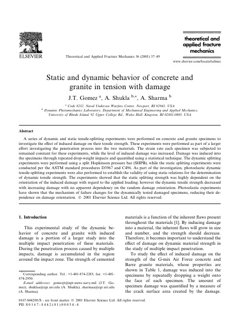
Static and dynamic behavior of concrete andgranite in tension with damageJ.T.Gomez a ,A.Shukla b,*,A.Sharma baCode 8232,Naval Undersea Warfare Center,Newport,RI 02841,USAbDynamic Photomechanics Laboratory,Department of Mechanical Engineering and Applied Mechanics,University of Rhode Island,92Upper College Rd.,Wales Hall,Kingston,RI 02881-0805,USAAbstractA series of dynamic and static tensile-splitting experiments were performed on concrete and granite specimens to investigate the e ect of induced damage on their tensile strength.These experiments were performed as part of a larger e ort investigating the penetration process into the two materials.The strain rate each specimen was subjected to remained constant for these experiments,while the level of induced damage was increased.Damage was induced into the specimens through repeated drop-weight impacts and quanti®ed using a statistical technique.The dynamic splitting experiments were performed using a split Hopkinson pressure bar (SHPB),while the static splitting experiments were conducted per the ASTM standard procedures D3967and C496.As part of the investigation,photoelastic dynamic tensile-splitting experiments were also performed to establish the validity of using static relations for the determination of dynamic tensile strength.The experiments showed that the static splitting strength was highly dependent on the orientation of the induced damage with regard to the applied loading;however the dynamic tensile strength decreased with increasing damage with no apparent dependency on the random damage orientation.Photoelastic experiments have shown that the mechanism of failure changes for the dynamically tested damaged specimens,reducing their de-pendence on damage orientation.Ó2001Elsevier Science Ltd.All rights reserved.1.IntroductionThis experimental study of the dynamic be-havior of concrete and granite with induced damage is a portion of a larger study into the multiple impact penetration of these materials.During the penetration process caused by multiple impacts,damage is accumulated in the region around the impact zone.The strength of cementedmaterials is a function of the inherent ¯aws present throughout the materials [1].By inducing damage into a material,the inherent ¯aws will grow in size and number,and the strength should decrease.Therefore,it becomes important to understand the e ect of damage on dynamic material strength in the study of multiple impact penetration.To study the e ect of induced damage on the strength of the G-mix Air Force concrete and Barre granite materials,whose properties are shown in Table 1,damage was induced into the specimens by repeatedly dropping a weight onto the face of each specimen.The amount of specimen damage was quanti®ed by a measure of the crack surface area created by thedamage.Theoretical and Applied Fracture Mechanics 36(2001)37±49/locate/tafmec*Corresponding author.Tel.:+1-401-874-2283;fax:+1-401-874-2950.E-mail addresses:gomezjt@ (J.T.Go-mez),shuklaa@ (A.Shukla),sharmaa@ (A.Sharma).0167-8442/01/$-see front matter Ó2001Elsevier Science Ltd.All rights reserved.PII:S 0167-8442(01)00054-4Photographs of the specimens were taken before and after the damage was induced.A grid of test lines was superimposed on the damaged specimen photograph,and the intercepts of the visible cracks with the grid lines were counted.The crack surface area per specimen volume was calculated using a statistical microscopy technique[2].The quasi-static tensile-splitting strengths of the damaged and undamaged specimens were deter-mined using ASTM standard procedures for both the concrete and granite specimens.To determine the dynamic tensile-splitting strength as a function of damage,a split Hopkin-son pressure bar(SHPB)was used to load the specimens diametrically with a dynamic stress wave.For these experiments it is assumed that the peak tensile-splitting stress of the specimen can be calculated from the peak transmitted compressive strain measured in the transmitter bar using the static relationshipfor sp litting stress,which is a function of load and specimen geometry[3].To ensure the validity of this assumption,photoelastic dynamic tensile-splitting experiments were per-formed on brittle,transparent polymer discs made of Homalite-100.The photoelastic experiments showed that the specimens were in equilibrium,i.e.the opposing contact loads were equal,for a relatively long pe-riod of time prior to failure.Also the experiments determined that once in equilibrium,the dynamic stress®eld in the specimen is identical to the stress ®eld in a statically loaded specimen.The experimental results showed that both the concrete and granite static tensile-splitting strength randomly decreased as the damage was increased, and in some cases remained unchanged in highly damaged specimens.In contrast,the dynamic ten-sile-splitting strength of the concrete and granite decreased in an orderly manner as the level of damage was increased.These results are due to the random orientation of the specimen in the loading apparatus.The static splitting strength was highly dependent on the damage orientation while the dynamic splitting strength was not.Photoelastic dynamic splitting experiments using damaged Ho-malite-100specimens determined that the failure mechanism of the damaged specimens changed, reducing their dependence on damage orientation as compared to statically tested specimens.2.Experimental procedure2.1.Quasi-static tensile-splitting experiments ASTM standard Brazilian,or tensile-splitting, experiments are usually performed on concrete or rock[4,5].For these types of materials it is di cult to fabricate and test typical``dog bone''speci-mens.The Brazilian tensile test was developed in order to indirectly determine the tensile strength of brittle materials using cylindrical specimens.Based on elasticity theory,the two-dimensional stress ®eld in the disc can be derived and then simpli®ed to examine only the stress along the loading line [6].Taking into account the specimen thickness,L, the stress distribution for the Brazilian splittingTable1Properties and composition of G-mix concrete and Barre graniteMaterial G-mix concrete Barre granite Compressive strength(MPa)41172.0Splitting tensile strength(MPa) 3.19.4Density(kg/m3)23372619 Composition Mixture for one cubic yard(kg)Mineral content(%)757.53/8-4Limestone36.5Plagioclase592.4Concrete sand31.9Quartz164.7Portland cement,type117.8Potash feldspar108.9Class``F''¯y ash8.0Biotite164.7Water 3.0Muscovite2.8Granophyre38J.T.Gomez et al./Theoretical and Applied Fracture Mechanics36(2001)37±49test is given by Eqs.(1),with parameters de®ned in Fig.1[1]:r x 2P p LD ;r y 2P p LD D 2y D Ày À1: 1 As shown,a constant tensile stress,r x ,is gener-ated along the loading line.At the contact points the elasticity solution is no longer valid due to the singularity of the loading.At these points there exists a bi-axial compressive stress of equivalent levels,which,along with the bearing blocks used to apply the load,allow the specimen to fail in tension along the loading line and not locally by compres-sion.Brittle materials,with a relatively low tensile strength compared to their compressive strength,will tend to fail in tension along the loading line.For each of the splitting tensile experiments the maximum load,P ,was used to calculate the split-ting stress,r x ,at failure using the ®rst of Eqs.(1).2.2.Split Hopkinson pressure bar for tensile-splitting In order to perform tensile splitting experiments under dynamic loading,an SHPB was used in compression.However,instead of sandwiching the specimen lengthwise,the specimen was held dia-metrically between the bars using steel bearing bars to avoid local failure due to the point load (Fig.2).To load the specimen,the incident bar is impacted with a projectile ®red from a gas gun,which creates a compressive wave traveling down the bar.At the specimen,this wave will be partially re¯ected back into the incident bar and partially transmitted into the transmitter bar.Strain gages mounted at the mid points of both bars are used to record the strain waves.Assuming one-dimen-sional propagation,and negligible attenuation of the waves,the loads on each end of the specimen can be calculated as a function of time with Eqs.(2)[7]:P 1 A b E b e i e r ;P 2 A b E b e t ;2where P 1and P 2are the loads on the incident and transmitted bar contact faces,respectively,A b is the bar cross-sectional area,E b is the Young's modulus of the bar material,and e i ,e r ,e t are the incident,re¯ected,and transmitted strain pulses shifted in time to account for the mid-bar location of the strain gages.For specimens in compression,the SHPB analysis assumes that the load on each specimen face is equal,so that the specimen is in equilib-rium.With this assumption the specimen stress/strain response can be calculated [7].However,for the dynamic splitting experiment the standard analysis to obtain the specimen stress can no longer be used.For these experiments it has been assumed that the peak tensile-splitting stress of the specimen is proportional to the peak transmitted compressive strain measured in the transmitter bar by the ®rst of Eqs.(1)[3],and that the load P is now de®ned by the second of Eqs.(2).For all these experiments,a 50.8mm diameter SHPB and 406.4mm long projectile were used.The concrete specimens wereapproximatelyJ.T.Gomez et al./Theoretical and Applied Fracture Mechanics 36(2001)37±493950.8mm in diameter and 21.8mm long.The granite specimens were approximately 55.1mm in diameter and 31.8mm long.Fig.3shows an un-damaged face for both the granite and concrete specimens.2.3.Photoelastic dynamic tensile-splitting experi-mentsPhotoelastic dynamic tensile-splitting experi-ments were performed on a brittle transparent material,Homalite-100,to determine the validity of using the static relations for dynamically loaded specimens (Fig.4).For the static relation to be valid,the specimen must be in equilibrium,i.e.the opposing contact loads must be equal.In similar experiments involving dynamic wave propagation in a chain of discs,it was shown that if the loading pulse width is much longer than the disc diameter,quasi-static stress ®eld equations were valid in a region close to the contact point [8].For the SHPB dynamic loading in this study,the incident pulse length is related to the projectile length.Therefore,all the photoelastic experiments were performed on a 12.7mm SHPB using a 203mm long projectile,giving a strain pulse of approximately 406mm in length.The gas gun pressure was initially varied from 0.207to 0.414MPa to deter-mine the pressure required to obtain fracture in the specimen.The specimens for all the dynamic splitting experiments were Homalite-100discs,25.4mm in diameter and 6.4mmthick.Fig.3.Undamaged G-mix concrete and Barre granitespecimens.40J.T.Gomez et al./Theoretical and Applied Fracture Mechanics 36(2001)37±492.4.Induced damage application and quanti®cation The concrete and granite specimens were tested both statically and dynamically as discussed earlier with increasing levels of induced damage.To in-duce damage in the specimens,a steel weight was dropped through a vented plastic tube,onto the specimen face.Each specimen was hit with multi-ple impacts until cracks were visible in the speci-men face.The amount of specimen damage was quanti-®ed by a measure of the crack surface area created by the damage.Photographs of the specimens were taken before and after the damage was induced.A grid of test lines was superimposed on the dam-aged specimen photograph,and the intercepts of the visible cracks with the grid lines were counted.A photograph of the grid lines being used to count the intercepts is shown in Fig.5.The crack surface area per specimen volume,S v ,is proportional to the number of intercepts by S v2N L ts2 number of interceptstest line length: 3The intercepts are counted as shown in Fig.5,and the test line length can be calculated as the lengthof grid lines that lie over the circular specimen.Forexample,for a 50mm diameter specimen the sys-tem of grid lines has a length of 1.014m.For the 46intercepts shown,the damage induced in the specimen would be 90.73m 2=m 3.This method was originally developed as a microscopy technique to study the ¯aws and grain boundaries of metal samples [2].For all the experiments,static and dynamic,no particular specimen orientation of the damage to the loading line was desired.The specimens were randomly oriented between the loading contacts.3.Results and discussion 3.1.Specimen equilibriumThe photoelastic experiments determined that,by subjecting the splitting specimen to a relatively long dynamic loading pulse in the SHPB,the specimen reaches equilibrium quickly and remains in equilibrium until fracture occurs.As shown (Fig.6),the wave front enters the specimen,loading only the incident contact (0l s).Both contact points of the specimen begin to be loaded when the wave travels across the specimen (10l s).When the contact loads become equal (30l s)the specimen is in equilibrium,and the photoelastic fringe patterns appear identical to a statically loaded specimen (Fig.7).These photoelastic fringe patterns are lines of constant maximum shear stress,and can be used to determine the stress ®elds in the specimens [9].Once the specimen is in equilibrium,the stress ®eld re¯ects back and forth increasing in magni-tude,as evident by the fringe patterns becoming more dense (50l s,Fig.6).The specimen remains in equilibrium until the time of failure (93l s).With this,the static stress relationship(Eqs.(1))is valid to determine the dynamic splitting strength of a specimen loaded in a SHPB with a relatively long projectile [10].3.2.Static tensile-splitting resultsAs shown,the static splitting strength of both the concrete (Fig.8)and the granite (Fig.9)asaFig.5.Grid lines superimposed over damaged specimen with intercepts highlighted.J.T.Gomez et al./Theoretical and Applied Fracture Mechanics 36(2001)37±4941function of damage randomly decreases to about half its virgin strength as the damage increases.However,in some cases the material retained its full strength even though the specimen was highly damaged.This is a result of the slowly developing stress ®eld being dependent on the damage orientation with respect to the loading line.As mentioned,the tensile-splitting test develops a constant tensile stress down the loading line of the specimen.If the damage cracks were parallel to the loading line,they would greatly decrease the strength.How-ever,if the damage cracks were perpendicular to the loading line,the cracks would close under thecompression in the y -direction and not a ect the splitting strength.This dependency on random damage orientation is evident in the static splitting results.3.3.Dynamic tensile-splitting resultsAs shown,the dynamic splitting strength for both the concrete (Fig.10)and the granite (Fig.11)decrease in an orderly fashion with increasing damage.This result shows that the random ori-entation of damage cracks in the specimens does not a ect the dynamic splitting strength as it did in the staticexperiments.Fig.6.Homalite-100specimen in dynamic tensile-splitting experiment.42J.T.Gomez et al./Theoretical and Applied Fracture Mechanics 36(2001)37±494.Photoelastic dynamic splitting experiments with damaged specimensTo examine the di erence between the static and dynamic splitting experiments with induced damage,a series of photoelastic dynamic splitting experiments was conducted using damaged Ho-malite-100specimens.The specimens,identical to the ones used previously in the equilibrium ex-periments,had a central crack initiated by tappinga short razor blade against the face.The amount of damage the cracks represented was quanti®ed using the method outlined earlier,and found to be approximately the same for each specimen.The projectile length and ®ring pressure also remained consistent with the earlier experiments.Four ad-ditional experiments were performed,two with the central crack parallel to the loading line,one with the crack oriented at an angle of 45°to the loading line,and one with the crack perpendicular to the loading line.The dynamic splitting strength of the Homa-lite-100,at an average strain rate of 200/s,dropped from 1.5times the static strengthforFig.7.Static Homalite-100tensile-splitting fringepattern.J.T.Gomez et al./Theoretical and Applied Fracture Mechanics 36(2001)37±4943the undamaged specimens to0.85times with the induced damage,with no orientation depen-dence.To examine the failure mechanisms of the un-damaged and damaged specimens the high-speed photography used to capture the fringe patterns was also used to examine crack propagation and specimen failure.Fig.12shows the typical failure of an undamaged dynamic splitting specimen made of Homalite-100.As shown,the splitting cracks form just outside a dark region near the contact point at approximately93l s from the initial specimen loading.Depending on the loading level one or more of the cracks propagate across the specimen causing failure.The dark regions at the loading points were found to be in-plane cracks that formed in the area of high compression stress near the contacts.These cracks tended to curve toward the surface and not cause the speci-men to fail.The crack initiation at the incident end of the specimen agrees with the experimental and numerical work performed on concrete by Tedesco et al.[11].Examining the failure of the0°damaged specimen(Fig.13),a change in the failure mechanism is evident.The central crack is unaf-fected by the initial passing of the wave front (10l s).However as the wave re¯ects back into the specimen creating the splitting stress®eld, stress concentration at the crack tips is evident with the formation of higher-order fringes(20l s). With the increased stress at the tip,the crack grows from each end of the damage toward the contact points(30l s).Once the cracks have reached the contact point the specimen has failed. Since the dynamic loading is still being applied, additional splitting cracks form at the contacts and travel through the specimen(70l s).The failure event in this case occurs in a much shorter period of time than the undamaged case,where the cracks were just beginning to form90l s after the initial loading.The splitting experiment performed with the central crack at45°to the loading line showed a similar failure pattern(Fig.14).The compressive wave front passes through the damaged area with no real e ect(10l s)until it re¯ects from the transmitter end and the tensile stress®eld begins to form.At this point we see fringe patterns around the crack tip,indicating an increase in stress (20l s).Again the cracks propagate from either side of the damage;however in this case the cracks are shown to move toward the contact points along the highest area of tensile stress(40l s).As with the0°damaged specimen,the dynamic loading is still being applied to the specimen,so once the cracks reach the contact points,addi-tional splitting cracks form(50l s).For the last experiment,the damaged specimen was placed in the SHPB to orient its central crack perpendicular to the loading line.In this con®g-uration it would be expected that the compressive stress in the specimen would cause the crack to close,and not lower the splitting strength.This is what caused the random changes in splitting strengths observed with the statically tested specimens.However,the photoelastic experiment showed that,similar to the other pre-damaged specimens,the crack initiation site was moved from the specimen incident end to the crack tips of the induced damage.Fig.15shows the crack propagation in the specimen.The wave enters the specimen and appears una ected by the damage, even after the initial re¯ection with no formation of fringes at the crack tips(0±20l s).After the next wave re¯ection,cracks can be seen initiating at the ends of the damage(40l s)and propagat-ing toward the contact points(50±60l s).Aswith 44J.T.Gomez et al./Theoretical and Applied Fracture Mechanics36(2001)37±49the other damaged specimens,failure occurs much earlier than in the undamaged specimens,where crack initiation occurs at approximately 93l s.5.ConclusionThe static and dynamic tensile-splitting exper-iments performed determined the e ect of induced levels of damage on the splitting strength of concrete and granite specimens.The static ex-periments showed that the splitting strength is highly dependent on the orientation of the dam-age with respect to the loading line.Damage cracks perpendicular to the loading line tend to be closed by the compressive stress in that direc-tion and do not e ect the strength.Damage cracks parallel to the loading line are opened by the tensile-splitting stress and decrease the strength drastically.Therefore,by randomly ori-enting the specimens in the testing machine,some specimens that were highly damaged may still have exhibited full strength if the major portion of its damage was oriented perpendicular to the loading line.In the dynamic case,the photoelastic experi-ments determined that the specimens wereinFig.12.Crack propagation of undamaged Homalite-100specimen subjected to dynamic splitting load in SHPB.J.T.Gomez et al./Theoretical and Applied Fracture Mechanics 36(2001)37±4945Fig.13.Crack propagation of damaged Homalite-100specimen with 0°central crack subjected to dynamic splitting load in SHPB.46J.T.Gomez et al./Theoretical and Applied Fracture Mechanics 36(2001)37±49equilibrium,and the dynamic stress ®eld resem-bled the static stress ®eld.This allows the use of the static stress ®eld relation to calculate the dy-namic splitting strength.For the concrete and granite specimens,the dynamic splitting strength was shown to decrease in a regular fashion with increasing damage without a dependency on the damage orientation.Additional photoelastic experiments were per-formed with damaged specimens containing a central crack,oriented at di erent angles to the loading line,parallel,45°,and perpendicular.The dynamic splitting strength of damaged specimens at an average strain rate of 200/s,dropped from 1.5times the static strength for the undamaged specimens to 0.85times with the induced dam-age,with no orientation dependence.The high-speed images of the specimen failure showed that in all cases the crack initiation moved from the incident end of the specimen to the edges of the specimen damage.The cracks then propagated along the line of maximum tensile stress toward the contact points.Crack initiation and specimen failure in the damaged specimens were also shown to occur in approximately 50l s,where the undamaged specimens experience crack initi-ation after 93l s.In the dynamic splitting experiments,the load in the specimen increases over time as the wave re¯ects back and forth [10].Since crack initiation and failure occur in a shorter period of time with the damaged specimens,there is less time for the load to increase.The calculated splitting stress,being a function of the load recorded in the transmitter bar,is therefore lower with more in-duced damage regardless of damageorientation.Fig.14.Crack propagation of damaged Homalite-100specimen with 45°central crack subjected to dynamic splitting load in SHPB.J.T.Gomez et al./Theoretical and Applied Fracture Mechanics 36(2001)37±4947。
- 1、下载文档前请自行甄别文档内容的完整性,平台不提供额外的编辑、内容补充、找答案等附加服务。
- 2、"仅部分预览"的文档,不可在线预览部分如存在完整性等问题,可反馈申请退款(可完整预览的文档不适用该条件!)。
- 3、如文档侵犯您的权益,请联系客服反馈,我们会尽快为您处理(人工客服工作时间:9:00-18:30)。
and Vsusy = 1 exp −ae−2κφ 4κ2 Ae2κφ + B + Ce−2κφ , (1.3)
Here g0 , g1 , Λ, a, A, B and C are constants and κ2 = 4πG is the D -dimensional gravitational constant. Eqns. (1.1)–(1.2) are somewhat more general than is demanded by string theory. However, if we set g0 = 1 we obtain the standard tree-level coupling between the dilaton and the electromagnetic field, while setting g1 = −1, Λ = (Dcrit − Deff ) /(3α′ ), in the Liouvilletype term (1.2) yields the case of a potential corresponding to a central charge deficit. The term (1.3), on the other hand, is the type of potential which arises in four dimensions from ¶ supersymmetry breaking via gaugino condensation in the hidden sector of the string theory [8]. Potentials of the form (1.2) and (1.3) have been widely studied in string cosmologies [9], but to date the only investigations of static spherically symmetric solutions involving such terms have been restricted to the case of uncharged solutions [10–14]. Maki and Shiraishi [15] have recently derived non-static Kastor-Traschen type [16] cosmological multi black hole solutions for the action (1.1)–(1.2). However, such solutions were only obtained for certain special values of the constants g0 , g1 and of the time-dependent coupling in the dilaton cosmological scale factor. In many respects the action (1.1) is still over-simplified because it neglects the possible contribution of additional scalar fields, such as the string moduli which correspond to the extra dimensions of spacetime after dimensional reduction. Static spherically symmetric solutions involving both moduli and a dilaton have been discussed recently by Cadoni and Mignemi [17], and by Cvetiˇ c and Tseytlin [18], but in the absence of a potential. The introduction of a potential greatly complicates the situation, however, as is well demonstrated by the case of the quadratic potential, where a complete integration proved impossible even numerically [7]. Given the inherent difficulties involved in studies of models with non-trivial potentials, the present paper is intended only as a first step: we will not study the problem posed by eqns. (1.1)–(1.3) in full, but will restrict ourselves solely to the case of a Liouville-type potential V = Vexp . It is our hope that a further refinement of the approach discussed here can be applied to the more difficult case when a supersymmetry-breaking potential of the type (1.3) is also included. We are of course most interested in the case D = 4, but will leave D arbitrary, (with the only requirement that D > 2), as this does not involve many extra complications. Furthermore, we will also leave the dilaton coupling to the electromagnetic field arbitrary, rather than immediately specialising to the string case (g0 = 1).
S.J. Poletti and D.L. t of Physics and Mathematical Physics, University of Adelaide, Adelaide, S.A. 5005, Australia.
ABSTRACT
We derive the global properties of static spherically symmetric solutions to the EinsteinMaxwell-dilaton system in the presence of an arbitrary exponential dilaton potential. We show that – with the exception of a pure cosmological constant ‘potential’ – no asymptotically flat, asymptotically de Sitter or asymptotically anti-de Sitter solutions exist in these models.
‡ A fascinating discussion of the observational consequences of a very weakly coupled massless dilaton is given in [5]. § Gregory and Harvey also considered a potential of the form V = 2m2 cosh2 φ. 2
⋆ E-mail: spoletti@.au † E-mail: dlw@.au 1
1. Introduction
There has been considerable interest recently in the properties of ‘stringy’ black holes: classical solutions of tree-level string effective actions, in which the Einstein action is supplemented by fields such as the axion, gauge fields, and the dilaton which couples in a non-trivial way to the other fields. In particular, dilaton black holes have been shown to have novel thermodynamic properties [1–3], and to behave like elementary particles in some scattering scenarios [4]. Unfortunately, much of the work on dilaton black holes to date has involved models with one serious deficiency: the dilaton has usually been assumed to be massless. It is widely believed, however, that the dilaton must aquire a mass through some symmetry breaking mechanism. Indeed, this is necessary in order to avoid long-range scalar forces which would ‡ otherwise arise . Gregory and Harvey [6] and Horne and Horowitz [7] have now finally made some investigation of black hole models which include a mass term – they have chosen a § standard quadratic potential for the dilaton field . While a rigorous proof of the existence of black hole solutions in these models has still to be given, the arguments of Horne and Horowitz [7] are nonetheless compelling. Ultimately, it would be physically desirable to investigate models of black holes in effective dilaton gravity theories in four dimensions which involve a dilaton potential generated by some specific symmetry breaking mechanism, rather than simply an ad hoc potential, as in the work to date [6,7]. In particular, one could consider an (Einstein frame) action such as S= √ dD x −g 1 1 R − g ab ∂a φ ∂b φ − V (φ) − exp 2 4κ D−2 4 −4g0 κφ D−2 Fab F ab , (1.1)