r语言t检验例题
R语言聚类分析、因子分析、t检验程序
R语言聚类分析、因子分析、t检验相关程序及程序运行结果相关程序:#####读入数据x=read.delim("G:\\上机考试数据.txt",header=TRUE,s=1)####作系统聚类d=dist(scale(x))hc1=hclust(d);hc1hc2=hclust(d,"average")hc3=hclust(d,"centroid")hc4=hclust(d,"ward")####绘出谱系图和聚类情况(最长距离法、类平均法)opar=par(mfrow=c(2,1),mar=c(5.2,4,0,0))plclust(hc1,hang=-1)re1=rect.hclust(hc1,k=3,border="red")plclust(hc2,hang=-1)re2=rect.hclust(hc2,k=3,border="red")par(opar)####绘出谱系图和聚类情况(重心法和Ward法)opar<-par(mfrow=c(2,1),mar=c(5.2,4,0,0))plclust(hc3,hang=-1)re3=rect.hclust(hc3,k=3,border="red")plclust(hc4,hang=-1)re4=rect.hclust(hc4,k=3,border="red")par(opar)####动态聚类法km<-kmeans(scale(x),3,nstart=35);kmsort(km$cluster)####因子分析y=read.delim("G:\\上机考试数据.txt",header=TRUE,s=1)R=cov(scale(y))fa<-factanal(factors=4,covmat=R);fa####计算因子得分y=read.delim("G:\\上机考试数据.txt",header=TRUE,s=1)fa<-factanal(~.,factors=4,data=y,scores="Bartlett");fafa$scores ####输出因子得分####画出散点图plot(fa$scores[,1:2],type="n")text(fa$scores[,1],fa$scores[,2])plot(fa$scores[,3:4],type="n")text(fa$scores[,3],fa$scores[,4])####t检验a1=fa$scores[,1]a2=fa$scores[,2]a3=fa$scores[,3]a4=fa$scores[,4]t.test(a1,a2,alternative="greater")t.test(a1,a3,alternative="greater")t.test(a1,a4,alternative="greater")t.test(a2,a3,alternative="greater")t.test(a2,a4,alternative="greater")t.test(a3,a4,alternative="greater")程序运行结果:> rm(list=ls(all=TRUE))> #####读入数据> x=read.delim("G:\\上机考试数据.txt",header=TRUE,s=1) > ####作系统聚类> d=dist(scale(x))> hc1=hclust(d);hc1Call:hclust(d = d)Cluster method : completeDistance : euclideanNumber of objects: 35> hc2=hclust(d,"average")> hc3=hclust(d,"centroid")> hc4=hclust(d,"ward")> ####绘出谱系图和聚类情况(最长距离法、类平均法)> opar=par(mfrow=c(2,1),mar=c(5.2,4,0,0))> plclust(hc1,hang=-1)> re1=rect.hclust(hc1,k=3,border="red")> plclust(hc2,hang=-1)> re2=rect.hclust(hc2,k=3,border="red")> par(opar)> ####绘出谱系图和聚类情况(重心法和Ward法)> opar<-par(mfrow=c(2,1),mar=c(5.2,4,0,0))> plclust(hc3,hang=-1)> re3=rect.hclust(hc3,k=3,border="red")> plclust(hc4,hang=-1)> re4=rect.hclust(hc4,k=3,border="red")> par(opar)> ####动态聚类法> km<-kmeans(scale(x),3,nstart=35);kmK-means clustering with 3 clusters of sizes 21, 6, 8Cluster means:工业生产总值.亿元. 财政收入.万元. 人均财政收入社会消费品零售总额.万元.1 -0.6065578 -0.6358116 -0.492914324 -0.387692232 0.7021330 0.9565806 1.730190783 0.061577083 1.0656146 0.9515700 -0.003742987 0.97150928外贸出口额外资利用总额.万美元. 新增固定资产投资.万元. 职工平均工资.元.1 -0.4402834 -0.6033739 -0.5009169 -0.59498172 0.4309513 1.4647875 0.8770164 1.47480543 0.8325306 0.4852659 0.6571445 0.4557230农民人均纯收入.元. 城镇固定资产投资人均固定资产投资万人拥有工业企业数量1 -0.5985518 -0.6641800 -0.50088606 -0.40066112 1.3534617 1.1106089 1.78476822 1.57153573 0.5561021 0.9105157 -0.02375026 -0.1269165 人均科教文卫.事业费支出1 -0.218176242 0.809047653 -0.03407311Clustering vector:长丰县肥东县肥西县天长市明光市来安县全椒县定远县3 3 3 3 1 1 1 1凤阳县当涂县庐江县无为县含山县和县芜湖县繁昌县1 2 1 3 1 3 2 2南陵县宁国市郎溪县广德县泾县绩溪县旌德县铜陵县3 2 1 2 1 1 1 2东至县石台县青阳县桐城市怀宁县枞阳县潜山县太湖县1 1 1 3 1 1 1 1宿松县望江县岳西县1 1 1Within cluster sum of squares by cluster:[1] 91.95071 40.32272 74.39793(between_SS / total_SS = 53.2 %)Available components:[1] "cluster" "centers" "totss" "withinss"[5] "tot.withinss" "betweenss" "size"> sort(km$cluster)明光市来安县全椒县定远县凤阳县庐江县含山县郎溪县1 1 1 1 1 1 1 1泾县绩溪县旌德县东至县石台县青阳县怀宁县枞阳县1 1 1 1 1 1 1 1潜山县太湖县宿松县望江县岳西县当涂县芜湖县繁昌县1 1 1 1 12 2 2宁国市广德县铜陵县长丰县肥东县肥西县天长市无为县2 2 23 3 3 3 3和县南陵县桐城市3 3 3>> ####因子分析> y=read.delim("G:\\上机考试数据.txt",header=TRUE,s=1)> R=cov(scale(y))> fa<-factanal(factors=4,covmat=R);faCall:factanal(factors = 4, covmat = R)Uniquenesses:工业生产总值.亿元. 财政收入.万元. 人均财政收入0.131 0.005 0.017 社会消费品零售总额.万元. 外贸出口额外资利用总额.万美元.0.135 0.757 0.466 新增固定资产投资.万元. 职工平均工资.元. 农民人均纯收入.元.0.278 0.249 0.228城镇固定资产投资人均固定资产投资万人拥有工业企业数量0.005 0.014 0.213 人均科教文卫.事业费支出0.518Loadings:Factor1 Factor2 Factor3 Factor4工业生产总值.亿元. 0.164 0.863 0.306财政收入.万元. 0.270 0.904 0.252 0.204人均财政收入0.911 0.257 0.236 0.177社会消费品零售总额.万元. -0.334 0.662 0.529 0.188外贸出口额0.144 0.255 0.396外资利用总额.万美元. 0.418 0.441 0.405新增固定资产投资.万元. 0.171 0.485 0.675职工平均工资.元. 0.669 0.446 0.322农民人均纯收入.元. 0.528 0.453 0.501 0.192城镇固定资产投资0.304 0.893 0.293 -0.142人均固定资产投资0.888 0.272 0.263 -0.231万人拥有工业企业数量0.838 0.271人均科教文卫.事业费支出0.659 -0.197Factor1 Factor2 Factor3 Factor4SS loadings 4.009 3.838 1.891 0.247Proportion Var 0.308 0.295 0.145 0.019Cumulative Var 0.308 0.604 0.749 0.768The degrees of freedom for the model is 32 and the fit was 1.9244>> ####计算因子得分> y=read.delim("G:\\上机考试数据.txt",header=TRUE,s=1)> fa<-factanal(~.,factors=4,data=y,scores="Bartlett");faCall:factanal(x = ~., factors = 4, data = y, scores = "Bartlett")Uniquenesses:工业生产总值.亿元. 财政收入.万元. 人均财政收入0.131 0.005 0.017 社会消费品零售总额.万元. 外贸出口额外资利用总额.万美元.0.135 0.757 0.466 新增固定资产投资.万元. 职工平均工资.元. 农民人均纯收入.元.0.278 0.249 0.228城镇固定资产投资人均固定资产投资万人拥有工业企业数量0.005 0.014 0.213 人均科教文卫.事业费支出0.518Loadings:Factor1 Factor2 Factor3 Factor4工业生产总值.亿元. 0.164 0.863 0.306财政收入.万元. 0.270 0.904 0.252 0.204人均财政收入0.911 0.257 0.236 0.177社会消费品零售总额.万元. -0.334 0.662 0.529 0.188外贸出口额0.144 0.255 0.396外资利用总额.万美元. 0.418 0.441 0.405新增固定资产投资.万元. 0.171 0.485 0.675职工平均工资.元. 0.669 0.446 0.322农民人均纯收入.元. 0.528 0.453 0.501 0.192城镇固定资产投资0.304 0.893 0.293 -0.142人均固定资产投资0.888 0.272 0.263 -0.231万人拥有工业企业数量0.838 0.271人均科教文卫.事业费支出0.659 -0.197Factor1 Factor2 Factor3 Factor4SS loadings 4.009 3.838 1.891 0.247Proportion Var 0.308 0.295 0.145 0.019Cumulative Var 0.308 0.604 0.749 0.768Test of the hypothesis that 4 factors are sufficient.The chi square statistic is 50.36 on 32 degrees of freedom.The p-value is 0.0206> fa$scores ####输出因子得分Factor1 Factor2 Factor3 Factor4 长丰县-0.183962645 1.07142140 -0.80273922 -0.55908770 肥东县-0.178091207 2.78806120 -1.86999699 0.68363597 肥西县0.348674595 3.12457544 -1.98272073 -0.50108034 天长市-0.328662939 0.11159589 1.52736647 0.46407338 明光市-0.963771018 -0.86354966 0.47002776 0.81176717 来安县-0.396419372 -0.49065354 0.31428314 -0.67509321 全椒县-0.127042257 -0.41988953 0.37755024 -0.37704456 定远县-1.024098347 -0.26034805 -0.17002711 -0.38265932凤阳县-0.688874840 -0.11971576 -0.14932367 0.36608860 当涂县0.703717153 1.67027029 0.79034965 0.31755372 庐江县-1.347580892 -0.10296382 1.40239214 0.73197698 无为县-1.808834990 1.38504818 2.96739685 -0.89328453 含山县-0.097182092 -0.62906939 -0.01725782 0.69586421 和县-0.633409518 -0.22667039 1.11273582 -0.23828640 芜湖县 1.465823581 0.20925937 0.70918377 -0.98730471 繁昌县 2.663194026 -0.03934722 -0.09699698 1.76758867 南陵县-0.121028895 -0.24059956 1.31746506 1.09467594 宁国市 2.176051304 0.26146591 2.18212596 0.98305592 郎溪县0.322546258 -0.51458155 -0.18277513 -2.09016770广德县0.458900888 0.38443902 1.34637112 -1.52375887 泾县0.066399254 -0.78667484 0.12591414 -0.17464409 绩溪县 1.630369791 -1.37642108 0.12958686 -1.09105223 旌德县0.015581604 -1.38966324 -0.22472503 -0.02326432铜陵县 2.352685506 0.08194171 -0.90854462 -1.71218909 东至县-0.420839170 -0.45254138 -0.45157759 0.05270322 石台县0.004431299 -1.12401413 -1.86938404 0.42232027 青阳县0.395060735 -0.98715620 -0.51665248 2.04123624 桐城市-0.359873784 0.44887271 0.56934952 0.74475186 怀宁县-0.022961863 0.38101100 -0.97991722 2.45423594 枞阳县-0.666759401 0.68399096 -1.01032266 -0.08880833 潜山县-0.659551399 -0.59777412 -0.59583407 0.51402884 太湖县-0.654810156 -0.58593199 -0.98967268 -0.43277938宿松县-0.920198188 -0.28228760 -0.27058925 -0.98831067 望江县-0.825113048 -0.70444337 -0.56674157 -0.10014261 岳西县-0.174369973 -0.40765667 -1.68629963 -1.30659888 > ####画出散点图> plot(fa$scores[,1:2],type="n")> text(fa$scores[,1],fa$scores[,2])> plot(fa$scores[,3:4],type="n")> text(fa$scores[,3],fa$scores[,4])>> ####t检验> a1=fa$scores[,1]> a2=fa$scores[,2]> a3=fa$scores[,3]> a4=fa$scores[,4]> t.test(a1,a2,alternative="greater")> t.test(a11,b11,alternative="greater")Welch Two Sample t-testdata: a11 and b11t = 1.9772, df = 9.704, p-value = 0.03855alternative hypothesis: true difference in means is greater than 0 95 percent confidence interval:0.06604808 Infsample estimates:mean of x mean of y0.9958313 0.1749454> t.test(a11,c11,alternative="greater")Welch Two Sample t-testdata: a11 and c11t = 4.3788, df = 9.086, p-value = 0.0008671alternative hypothesis: true difference in means is greater than 0 95 percent confidence interval:1.039104 Infsample estimates:mean of x mean of y0.9958313 -0.7901305> t.test(b11,c11,alternative="greater")Welch Two Sample t-testdata: b11 and c11t = 5.8762, df = 21.925, p-value = 3.299e-06alternative hypothesis: true difference in means is greater than 0 95 percent confidence interval:0.6830173 Infsample estimates:mean of x mean of y0.1749454 -0.7901305> t.test(a12,b12,alternative="greater")Welch Two Sample t-testdata: a12 and b12t = 2.994, df = 10.814, p-value = 0.006212alternative hypothesis: true difference in means is greater than 0 95 percent confidence interval:0.5557607 Infsample estimates:mean of x mean of y0.9931852 -0.3988946> t.test(a12,c12,alternative="greater")Welch Two Sample t-testdata: a12 and c12t = 2.5917, df = 10.145, p-value = 0.01329alternative hypothesis: true difference in means is greater than 0 95 percent confidence interval:0.356743 Infsample estimates:mean of x mean of y0.9931852 -0.1893416> t.test(b12,c12,alternative="greater")Welch Two Sample t-testdata: b12 and c12t = -0.8809, df = 22.84, p-value = 0.8062alternative hypothesis: true difference in means is greater than 0 95 percent confidence interval:-0.6173701 Inf sample estimates:mean of x mean of y -0.3988946 -0.1893416。
t检验法的详细步骤例题

t检验法的详细步骤例题
假设我们想要通过t检验法来判断男生和女生在数学考试成绩上是否存在显著差异。
以下是一个详细步骤的例题:
步骤1: 建立假设(Hypotheses)
- 零假设(H0):男生和女生在数学考试成绩上没有差异,即两个样本的均值相等。
- 对立假设(H1):男生和女生在数学考试成绩上存在差异,即两个样本的均值不相等。
步骤2: 收集样本数据
- 随机抽取一定数量的男生和女生学生作为样本,记录他们在数学考试中的成绩。
步骤3: 计算统计量
- 对于两个独立样本的t检验,统计量t的计算公式为: t = (x1-x2) / sqrt(s1^2/n1 + s2^2/n2)
其中,x1和x2是两个样本的平均值,s1和s2是两个样本的标准差,n1和n2是两个样本的样本容量。
步骤4: 设置显著性水平
- 根据实际情况和问题的重要性,选择一个显著性水平(例如α = 0.05或α = 0.01)。
步骤5: 计算临界值
- 在给定的显著性水平下,查表或使用统计软件来计算临界值。
对于双尾检验,需要计算两侧的临界值。
步骤6: 做出决策
- 比较统计量t与临界值。
如果统计量t的绝对值大于临界值,就拒绝零假设,即表明男生和女生在数学考试成绩上存在显著差异;否则就接受零假设,认为差异不显著。
步骤7: 得出结论
- 根据统计推断的结果,结合具体问题,得出是否拒绝零假设的结论,并解释结果的意义。
R语言聚类分析、因子分析、t检验程序
R语言聚类分析、因子分析、t检验相关程序及程序运行结果相关程序: #####读入数据x=read.delim("G:\\上机考试数据.txt",header=TRUE,s=1####作系统聚类d=dist(scale(xhc1=hclust(d;hc1hc2=hclust(d,"average"hc3=hclust(d,"centroid"hc4=hclust(d,"ward"####绘出谱系图和聚类情况(最长距离法、类平均法opar=par(mfrow=c(2,1,mar=c(5.2,4,0,0plclust(hc1,hang=-1re1=rect.hclust(hc1,k=3,border="red"plclust(hc2,hang=-1re2=rect.hclust(hc2,k=3,border="red"par(opar####绘出谱系图和聚类情况(重心法和Ward法opar<-par(mfrow=c(2,1,mar=c(5.2,4,0,0plclust(hc3,hang=-1re3=rect.hclust(hc3,k=3,border="red"plclust(hc4,hang=-1re4=rect.hclust(hc4,k=3,border="red"par(opar####动态聚类法km<-kmeans(scale(x,3,nstart=35;kmsort(km$cluster####因子分析y=read.delim("G:\\上机考试数据.txt",header=TRUE,s=1 R=cov(scale(yfa<-factanal(factors=4,covmat=R;fa####计算因子得分y=read.delim("G:\\上机考试数据.txt",header=TRUE,s=1 fa<-factanal(~.,factors=4,data=y,scores="Bartlett";fafa$scores ####输出因子得分####画出散点图plot(fa$scores[,1:2],type="n"text(fa$scores[,1],fa$scores[,2]plot(fa$scores[,3:4],type="n"text(fa$scores[,3],fa$scores[,4]####t检验a1=fa$scores[,1]a2=fa$scores[,2]a3=fa$scores[,3]a4=fa$scores[,4]t.test(a1,a2,alternative="greater"t.test(a1,a3,alternative="greater"t.test(a1,a4,alternative="greater"t.test(a2,a3,alternative="greater"t.test(a2,a4,alternative="greater"t.test(a3,a4,alternative="greater"程序运行结果:> rm(list=ls(all=TRUE> #####读入数据> x=read.delim("G:\\上机考试数据.txt",header=TRUE,s=1 > ####作系统聚类> d=dist(scale(x> hc1=hclust(d;hc1Call:hclust(d = dCluster method : completeDistance : euclideanNumber of objects: 35> hc2=hclust(d,"average"> hc3=hclust(d,"centroid"> hc4=hclust(d,"ward"> ####绘出谱系图和聚类情况(最长距离法、类平均法> opar=par(mfrow=c(2,1,mar=c(5.2,4,0,0> plclust(hc1,hang=-1> re1=rect.hclust(hc1,k=3,border="red"> plclust(hc2,hang=-1> re2=rect.hclust(hc2,k=3,border="red"> par(opar> ####绘出谱系图和聚类情况(重心法和Ward法> opar<-par(mfrow=c(2,1,mar=c(5.2,4,0,0> plclust(hc3,hang=-1> re3=rect.hclust(hc3,k=3,border="red"> plclust(hc4,hang=-1> re4=rect.hclust(hc4,k=3,border="red"> par(opar> ####动态聚类法> km<-kmeans(scale(x,3,nstart=35;kmK-means clustering with 3 clusters of sizes 21, 6, 8Cluster means:工业生产总值.亿元. 财政收入.万元. 人均财政收入社会消费品零售总额.万元.1 -0.6065578 -0.6358116 -0.492914324 -0.387692232 0.7021330 0.9565806 1.730190783 0.061577083 1.0656146 0.9515700 -0.003742987 0.97150928外贸出口额外资利用总额.万美元. 新增固定资产投资.万元. 职工平均工资.元.1 -0.4402834 -0.6033739 -0.5009169 -0.59498172 0.4309513 1.4647875 0.8770164 1.47480543 0.8325306 0.4852659 0.6571445 0.4557230农民人均纯收入.元. 城镇固定资产投资人均固定资产投资万人拥有工业企业数量1 -0.5985518 -0.6641800 -0.50088606 -0.40066112 1.3534617 1.1106089 1.78476822 1.57153573 0.5561021 0.9105157 -0.02375026 -0.1269165 人均科教文卫.事业费支出1 -0.218176242 0.809047653 -0.03407311Clustering vector:长丰县肥东县肥西县天长市明光市来安县全椒县定远县3 3 3 3 1 1 1 1凤阳县当涂县庐江县无为县含山县和县芜湖县繁昌县1 2 1 3 1 3 2 2南陵县宁国市郎溪县广德县泾县绩溪县旌德县铜陵县3 2 1 2 1 1 1 2东至县石台县青阳县桐城市怀宁县枞阳县潜山县太湖县1 1 1 3 1 1 1 1宿松县望江县岳西县1 1 1Within cluster sum of squares by cluster:[1] 91.95071 40.32272 74.39793(between_SS / total_SS = 53.2 %Available components:[1] "cluster" "centers" "totss" "withinss"[5] "tot.withinss" "betweenss" "size"> sort(km$cluster明光市来安县全椒县定远县凤阳县庐江县含山县郎溪县1 1 1 1 1 1 1 1泾县绩溪县旌德县东至县石台县青阳县怀宁县枞阳县1 1 1 1 1 1 1 1潜山县太湖县宿松县望江县岳西县当涂县芜湖县繁昌县1 1 1 1 12 2 2宁国市广德县铜陵县长丰县肥东县肥西县天长市无为县2 2 23 3 3 3 3和县南陵县桐城市3 3 3>> ####因子分析> y=read.delim("G:\\上机考试数据.txt",header=TRUE,s=1> R=cov(scale(y> fa<-factanal(factors=4,covmat=R;faCall:factanal(factors = 4, covmat = RUniquenesses:工业生产总值.亿元. 财政收入.万元. 人均财政收入0.131 0.005 0.017 社会消费品零售总额.万元. 外贸出口额外资利用总额.万美元.0.135 0.757 0.466 新增固定资产投资.万元. 职工平均工资.元. 农民人均纯收入.元.0.278 0.249 0.228城镇固定资产投资人均固定资产投资万人拥有工业企业数量0.005 0.014 0.213 人均科教文卫.事业费支出0.518Loadings:Factor1 Factor2 Factor3 Factor4工业生产总值.亿元. 0.164 0.863 0.306财政收入.万元. 0.270 0.904 0.252 0.204人均财政收入0.911 0.257 0.236 0.177社会消费品零售总额.万元. -0.334 0.662 0.529 0.188外贸出口额0.144 0.255 0.396外资利用总额.万美元. 0.418 0.441 0.405新增固定资产投资.万元. 0.171 0.485 0.675职工平均工资.元. 0.669 0.446 0.322农民人均纯收入.元. 0.528 0.453 0.501 0.192城镇固定资产投资0.304 0.893 0.293 -0.142人均固定资产投资0.888 0.272 0.263 -0.231万人拥有工业企业数量0.838 0.271人均科教文卫.事业费支出0.659 -0.197Factor1 Factor2 Factor3 Factor4SS loadings 4.009 3.838 1.891 0.247Proportion Var 0.308 0.295 0.145 0.019Cumulative Var 0.308 0.604 0.749 0.768The degrees of freedom for the model is 32 and the fit was 1.9244 >> ####计算因子得分> y=read.delim("G:\\上机考试数据.txt",header=TRUE,s=1> fa<-factanal(~.,factors=4,data=y,scores="Bartlett";faCall:factanal(x = ~., factors = 4, data = y, scores = "Bartlett"Uniquenesses:工业生产总值.亿元. 财政收入.万元. 人均财政收入0.131 0.005 0.017 社会消费品零售总额.万元. 外贸出口额外资利用总额.万美元.0.135 0.757 0.466 新增固定资产投资.万元. 职工平均工资.元. 农民人均纯收入.元.0.278 0.249 0.228城镇固定资产投资人均固定资产投资万人拥有工业企业数量0.005 0.014 0.213 人均科教文卫.事业费支出0.518Loadings:Factor1 Factor2 Factor3 Factor4工业生产总值.亿元. 0.164 0.863 0.306财政收入.万元. 0.270 0.904 0.252 0.204人均财政收入0.911 0.257 0.236 0.177社会消费品零售总额.万元. -0.334 0.662 0.529 0.188外贸出口额0.144 0.255 0.396外资利用总额.万美元. 0.418 0.441 0.405新增固定资产投资.万元. 0.171 0.485 0.675职工平均工资.元. 0.669 0.446 0.322农民人均纯收入.元. 0.528 0.453 0.501 0.192城镇固定资产投资0.304 0.893 0.293 -0.142人均固定资产投资0.888 0.272 0.263 -0.231万人拥有工业企业数量0.838 0.271人均科教文卫.事业费支出 0.659 -0.197 Factor1 Factor2 Factor3 Factor4 SS loadings 4.009 3.838 Proportion Var 0.308 0.295 Cumulative Var 0.308 0.604 1.8910.145 0.749 0.247 0.019 0.768 Test of the hypothesis that 4 factors are sufficient. The chi square statistic is 50.36 on 32 degrees of freedom. The p-value is 0.0206 > fa$scores####输出因子得分 Factor1 Factor2 Factor3 Factor4 长丰县 -0.183962645 1.07142140 -0.80273922 -0.55908770 肥东县 -0.178091207 2.78806120 -1.86999699 0.68363597 肥西县 0.348674595 3.12457544 -1.98272073 -0.50108034 天长市 -0.3286629390.11159589 1.52736647 0.46407338 明光市 -0.963771018 -0.86354966 0.47002776 0.81176717 来安县 -0.396419372 -0.49065354 0.31428314 -0.67509321 全椒县 -0.127042257 -0.41988953 0.37755024 -0.37704456 定远县 -1.024098347 -0.26034805 -0.17002711 -0.38265932 凤阳县 -0.688874840 -0.11971576 -0.14932367 0.36608860 当涂县 0.703717153 1.67027029 0.79034965 0.31755372 庐江县 -1.347580892 -0.10296382 1.40239214 0.73197698 无为县 -1.808834990 1.38504818 2.96739685 -0.89328453 含山县 -0.097182092 -0.62906939 -0.01725782 0.69586421 和县 -0.633409518 -0.22667039 1.11273582 -0.23828640 芜湖县 1.465823581 0.20925937 0.70918377 -0.98730471 繁昌县 2.663194026 -0.03934722 -0.09699698 1.76758867 南陵县 -0.121028895 -0.24059956 1.31746506 1.09467594 宁国市 2.1760513040.26146591 2.18212596 0.98305592 郎溪县 0.322546258 -0.51458155 -0.18277513 -2.09016770 广德县 0.458900888 0.38443902 1.34637112 -1.52375887 泾县0.066399254 -0.78667484 0.12591414 -0.17464409 绩溪县 1.630369791 -1.37642108 0.12958686 -1.09105223 旌德县 0.015581604 -1.38966324 -0.22472503 -0.02326432 铜陵县 2.352685506 0.08194171 -0.90854462 -1.71218909 东至县 -0.420839170 -0.45254138 -0.45157759 0.05270322 石台县 0.004431299 -1.12401413 -1.86938404 0.42232027 青阳县 0.395060735 -0.98715620 -0.51665248 2.04123624 桐城市 -0.359873784 0.44887271 0.56934952 0.74475186 怀宁县 -0.022961863 0.38101100 -0.97991722 2.45423594 枞阳县 -0.666759401 0.68399096 -1.01032266 -0.08880833 潜山县 -0.659551399 -0.59777412 -0.59583407 0.51402884 太湖县 -0.654810156 -0.58593199 -0.98967268 -0.43277938宿松县 -0.920198188 -0.28228760 -0.27058925 -0.98831067 望江县 -0.825113048 -0.70444337 -0.56674157 -0.10014261 岳西县 -0.174369973 -0.40765667 -1.68629963 -1.30659888 > ####画出散点图 > plot(fa$scores[,1:2],type="n" >text(fa$scores[,1],fa$scores[,2] > plot(fa$scores[,3:4],type="n" >text(fa$scores[,3],fa$scores[,4] > > ####t 检验 > a1=fa$scores[,1] > a2=fa$scores[,2] > a3=fa$scores[,3] > a4=fa$scores[,4] > t.test(a1,a2,alternative="greater" >t.test(a11,b11,alternative="greater" Welch Two Sample t-test data: a11 and b11 t =1.9772, df = 9.704, p-value = 0.03855 alternative hypothesis: true difference in means is greater than 0 95 percent confidence interval: 0.06604808 Inf sample estimates: mean of x mean of y 0.9958313 0.1749454 > t.test(a11,c11,alternative="greater" Welch Two Sample t-test data: a11 and c11 t = 4.3788, df = 9.086, p-value = 0.0008671 alternative hypothesis: true difference in means is greater than 0 95 percent confidence interval:1.039104 Inf sample estimates: mean of x mean of y 0.9958313 -0.7901305 >t.test(b11,c11,alternative="greater" Welch Two Sample t-testdata: b11 and c11 t = 5.8762, df = 21.925, p-value = 3.299e-06 alternative hypothesis: true difference in means is greater than 0 95 percent confidence interval:0.6830173 Inf sample estimates: mean of x mean of y 0.1749454 -0.7901305 >t.test(a12,b12,alternative="greater" Welch Two Sample t-test data: a12 and b12 t = 2.994, df = 10.814, p-value = 0.006212 alternative hypothesis: true difference in means is greater than 0 95 percent confidence interval: 0.5557607 Inf sample estimates: mean of x mean of y 0.9931852 -0.3988946 > t.test(a12,c12,alternative="greater" Welch Two Sample t-test data: a12 and c12 t = 2.5917, df = 10.145, p-value = 0.01329 alternative hypothesis: true difference in means is greater than 0 95 percent confidence interval:0.356743 Inf sample estimates: mean of x mean of y 0.9931852 -0.1893416 >t.test(b12,c12,alternative="greater" Welch Two Sample t-test data: b12 and c12 t = -0.8809, df = 22.84, p-value = 0.8062 alternative hypothesis: true difference in means is greater than 0 95 percent confidence interval:-0.6173701 Inf sample estimates: mean of x mean of y -0.3988946 -0.1893416。
R语言各种假设检验实例整理(常用)
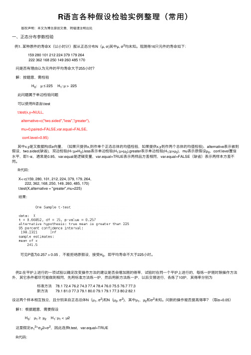
R语⾔各种假设检验实例整理(常⽤)版权声明:本⽂为博主原创⽂章,转载请注明出处⼀、正态分布参数检验例1. 某种原件的寿命X(以⼩时计)服从正态分布N(µ, σ)其中µ, σ2均未知。
现测得16只元件的寿命如下:159 280 101 212 224 379 179 264222 362 168 250 149 260 485 170问是否有理由认为元件的平均寿命⼤于255⼩时?解:按题意,需检验H0: µ ≤ 225H1: µ >225此问题属于单边检验问题可以使⽤R语⾔t.testt.test(x,y=NULL,alternative=c("two.sided","less","greater"),mu=0,paired=FALSE,var.equal=FALSE,conf.level=0.95)其中x,y是⼜数据构成e向量,(如果只提供x,则作单个正态总体的均值检验,如果提供x,y则作两个总体的均值检验),alternative表⽰被则假设,two.sided(缺省),双边检验(H1:µ≠H0),less表⽰单边检验(H1:µ<µ0),greater表⽰单边检验(H1:µ>µ0),mu表⽰原假设µ0,conf.level置信⽔平,即1-α,通常是0.95,var.equal是逻辑变量,var.equal=TRUE表⽰两样品⽅差相同,var.equal=FALSE(缺省)表⽰两样本⽅差不同。
R代码:X<-c(159, 280, 101, 212, 224, 379, 179, 264,222, 362, 168, 250, 149, 260, 485, 170)t.test(X,alternative = "greater",mu=225)结果:可见P值为0.257 > 0.05 ,不能拒绝原假设,接受H0,即平均寿命不⼤于225⼩时。
t检验例题解析
t检验例题解析摘要:1.引言2.t检验的原理和方法3.例题解析4.结论与启示正文:**引言**在统计分析中,t检验是一种常用的方法,用于检验两组数据之间是否存在显著差异。
t检验的原理和步骤相对简单,但其在实际应用中的正确性和实用性却非常重要。
本文将通过例题解析的方式,帮助你更好地理解和掌握t检验的方法和技巧。
**t检验的原理和方法**t检验主要包括两种类型:独立样本t检验(比较两组独立样本)和配对样本t检验(比较同一组样本的两个时间点)。
其基本步骤如下:1.建立原假设:H0表示两组样本的均值相等,H1表示存在显著差异。
2.收集数据并计算统计量:如平均值、标准差等。
3.计算t值:t = (样本均值差- 总体均值差)/ 标准误差。
4.计算p值:根据t值和自由度(df)查找t分布表,得到p值。
5.判断结论:如果p值小于显著性水平(通常为0.05),则拒绝原假设,认为存在显著差异。
**例题解析**例题1:比较两组独立样本的均值差异。
数据如下:样本1:均值= 50,标准差= 10样本2:均值= 55,标准差= 10假设检验:H0:μ1 = μ2,H1:μ1 ≠ μ2计算过程:1.计算t值:t = (50 - 55) / sqrt((10^2 + 10^2) / 2) = -2.52.计算p值:p = 2 * (1 - (1 - 0.025) / 2) = 0.0253.结论:p值小于0.05,拒绝原假设,认为两组样本存在显著差异。
例题2:比较同一组样本的两个时间点的均值差异。
数据如下:时间1:均值= 50,标准差= 10时间2:均值= 55,标准差= 10假设检验:H0:μ1 = μ2,H1:μ1 ≠ μ2计算过程:1.计算t值:t = (50 - 55) / sqrt((10^2 + 10^2) / 2) = -2.52.计算p值:p = 2 * (1 - (1 - 0.025) / 2) = 0.0253.结论:p值小于0.05,拒绝原假设,认为同一组样本的两个时间点存在显著差异。
r语言t检验 相关检验案例代码
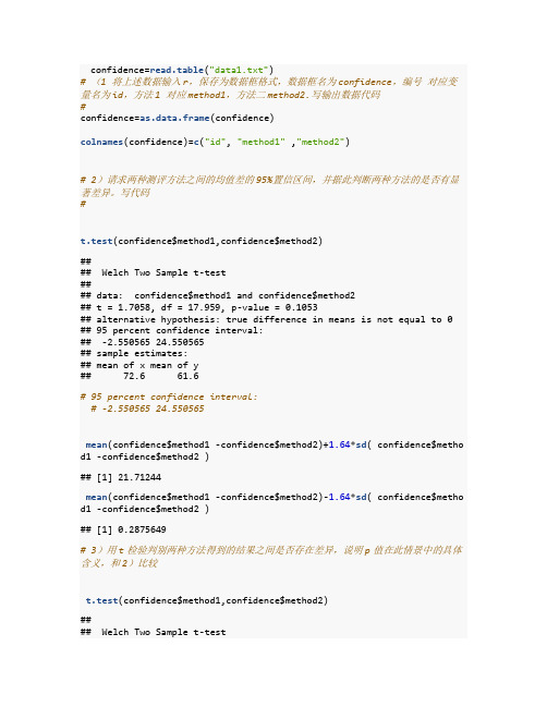
confidence=read.table("data1.txt")# (1 将上述数据输入r,保存为数据框格式,数据框名为confidence,编号对应变量名为id,方法1 对应method1,方法二method2.写输出数据代码#confidence=as.data.frame(confidence)colnames(confidence)=c("id", "method1" ,"method2")# 2)请求两种测评方法之间的均值差的95%置信区间,并据此判断两种方法的是否有显著差异。
写代码#t.test(confidence$method1,confidence$method2)#### Welch Two Sample t-test#### data: confidence$method1 and confidence$method2## t = 1.7058, df = 17.959, p-value = 0.1053## alternative hypothesis: true difference in means is not equal to 0 ## 95 percent confidence interval:## -2.550565 24.550565## sample estimates:## mean of x mean of y## 72.6 61.6# 95 percent confidence interval:# -2.550565 24.550565mean(confidence$method1 -confidence$method2)+1.64*sd( confidence$method 1 -confidence$method2 )## [1] 21.71244mean(confidence$method1 -confidence$method2)-1.64*sd( confidence$method 1 -confidence$method2 )## [1] 0.2875649# 3)用t检验判别两种方法得到的结果之间是否存在差异,说明p值在此情景中的具体含义,和2)比较t.test(confidence$method1,confidence$method2)#### Welch Two Sample t-test#### data: confidence$method1 and confidence$method2## t = 1.7058, df = 17.959, p-value = 0.1053## alternative hypothesis: true difference in means is not equal to 0 ## 95 percent confidence interval:## -2.550565 24.550565## sample estimates:## mean of x mean of y## 72.6 61.6#p值大于0.05,因此结果之间不存在差异# p值是在假两种方法没有差异为真时,得到与样本相同或者更极端的结果的概率。
R语言中的t-test和ANOVA_13965

score mean Z standard deviation
Shrinking drug (non-effect value=64)
Vasishth’s Height Example
大部分情况下我们并不知道σ ——T分布
> pt(-3.02, df = 10) + (1 - pt(3.02, df = 10)) [1] 0.01289546
> n <- length(mpg)
> t.test(mpg,mu=17,alternative="less") > c(xbar, s, n)
[1] 14.870000 1.572012 10.000000 > SE <- s/sqrt(n)
> (xbar - 17)/SE
[1] -4.284732 > pt(-4.285, df = 9, lower.tail = T) [1] 0.001017478
两正态总体参数检验
> x<-c(20.5, 19.8, 19.7, 20.4, 20.1, 20.0, 19.0, 19.9) > y<-c(20.7, 19.8, 19.5, 20.8, 20.4, 19.6, 20.2) > t.test(x, y, var.equal=TRUE) Two Sample t-test data: x and y t = -0.8548, df = 13, p-value = 0.4081 alternative hypothesis: true difference in means is not equal to 0 95 percent confidence interval: -0.7684249 0.3327106 sample estimates: mean of x mean of y 19.92500 20.14286
R语言t检验和非正态性的鲁棒性

R语言t检验和非正态性的鲁棒性原文连接:/?p=6261t检验是统计学中最常用的检验之一。
双样本t检验允许我们基于来自两组中的每一组的样本来测试两组的总体平均值相等的零假设。
这在实践中意味着什么?如果我们的样本量不是太小,如果我们的数据看起来违反了正常假设,我们就不应过分担心。
此外,出于同样的原因,即使X不正常(同样,当样本量足够大时),组均值差异的95%置信区间也将具有正确的覆盖率。
当然,对于小样本或高度偏斜的分布,上述渐近结果可能不会给出非常好的近似,因此类型1误差率可能偏离标称的5%水平。
现在让我们用R来检验样本均值分布(在重复样本中)收敛到正态分布的速度。
我们将模拟来自对数正态分布的数据- 即log(X)遵循正态分布。
我们可以通过从正态分布中取幂随机抽取来从此分布中生成随机样本。
首先,我们将绘制一个大的(n = 100000)样本并绘制其分布以查看它的外观:我们可以看到它的分布是高度偏斜的。
从表面上看,我们会担心对这些数据使用t检验,假设X是正态分布的。
为了看看样本的样本分布,我们将选择样本大小为n,并从对数正态分布中重复绘制大小为n的样本,计算样本均值,然后绘制这些样本均值的分布。
以下显示n = 3的样本平均值的直方图(来自10,000个重复样本):样本均值的分布,n = 3这里的采样分布是倾斜的。
如此小的样本量,如果其中一个样本从分布的尾部具有高值,则这将给出与真实均值相差很远的样本均值。
如果我们重复,但现在n = 10:它现在看起来更正常,但它仍然是偏斜的 - 样本均值有时很大。
请注意,x轴范围现在更小 - 样本均值的可变性现在小于n = 3。
最后,我们尝试n = 100:现在样本均值的分布(来自人口的重复样本)看起来非常正常。
当n很大时,即使我们的一个观测结果可能位于分布的尾部,分布中心附近的所有其他观测值也会保持平均值。
这表明对于这个特定的X 分布,t检验应该是正确的,n = 100 。
- 1、下载文档前请自行甄别文档内容的完整性,平台不提供额外的编辑、内容补充、找答案等附加服务。
- 2、"仅部分预览"的文档,不可在线预览部分如存在完整性等问题,可反馈申请退款(可完整预览的文档不适用该条件!)。
- 3、如文档侵犯您的权益,请联系客服反馈,我们会尽快为您处理(人工客服工作时间:9:00-18:30)。
r语言t检验例题
如何理解r语言t检验例题
例题,遗传算法(GeneticAlgorithm)是一种基于自然选择模拟进化机制的算法,通过对个体间竞争或协作、变异和遗传实现目标优化求解。
主要包括种群初始化、选择和变异、遗传迭代等步骤,能够很好地应用于简单或复杂的求解问题上。
例题检验,通常,例题检验指的是一种研究方法,它利用小规模的试题或案例来测试和验证某种理论或假设。
这种检验可以实施一系列步骤,其中包括收集例题数据、对假设进行建模、应用统计分析等,最后形成结论。
例题检验通常是在一个更大的实验中完成的,例如,在一个企业发展计划中,用例题检验来决定计划是否可行。
r语言t检验例题,假设有一组数据,20个男性和20个女性的身高分别记录在表中:
| 性别 | 身高(cm) |
| --- | ---------- |
| 男 | 172 |
| 女 | 158 |
| 男 | 176 |
| 女 | 167 |
| 男 | 187 |
| 女 | 149 |
| 男 | 159 |
| 女 | 151 |
| ... | ... |
要检验两性之间身高是否存在显著差异,使用 R 语言可以使用 t 检验:
为什么需要r语言t检验例题
1. 检验某种假设是否成立。
2. 批判性和客观地评估数据。
3. 确定总体参数是否有效。
怎么进一步推进完成r语言t检验例题
一、针对性地掌握t检验的相关基础知识,如t统计量、特征参数、抽样分布、假设检验、显著性水平等。
二、通过阅读和实践,学习r语言中t检验的应用,如如何使用t检验方法检
验两组样本的均值是否不同、如何使用t检验方法检验单样本的均值和总体均
值是否不同等。
三、练习针对t检验的实际例题,根据所提供的数据计算t统计量、计算抽样
分布的参数、进行假设检验等。
四、解决t检验实际例题时,可以多使用r语言编程过程,包括数据准备、t
检验分析和结果展示。
五、总结学习经验,查阅有关文献,不断学习t检验的先进理论和实践技能,
充分发挥R语言在t检验中的优势。