Estimation of safety distances in the vicinity of fuel gas pipelines

合集下载

Triangulation

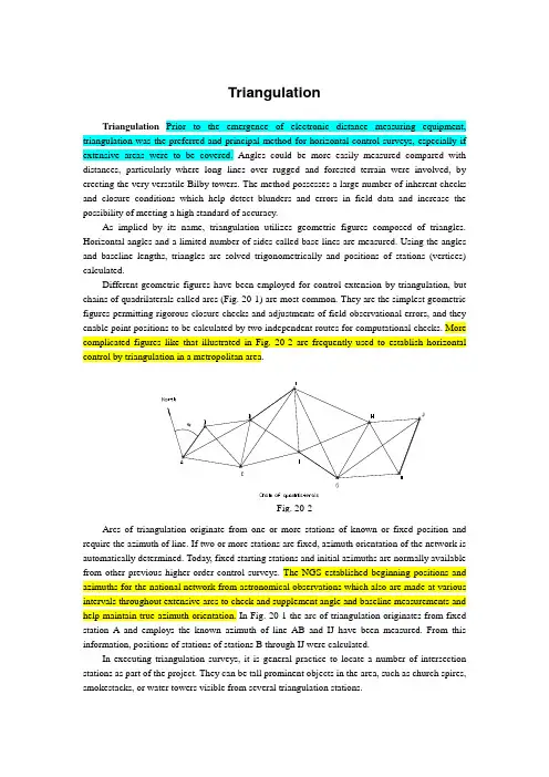
TriangulationTriangulation Prior to the emergence of electronic distance measuring equipment, triangulation was the preferred and principal method for horizontal control surveys, especially if extensive areas were to be covered. Angles could be more easily measured compared with distances, particularly where long lines over rugged and forested terrain were involved, by erecting the very versatile Bilby towers. The method possesses a large number of inherent checks and closure conditions which help detect blunders and errors in field data and increase the possibility of meeting a high standard of accuracy.As implied by its name, triangulation utilizes geometric figures composed of triangles. Horizontal angles and a limited number of sides called base lines are measured. Using the angles and baseline lengths, triangles are solved trigonometrically and positions of stations (vertices) calculated.Different geometric figures have been employed for control extension by triangulation, but chains of quadrilaterals called arcs (Fig. 20-1) are most common. They are the simplest geometric figures permitting rigorous closure checks and adjustments of field observational errors, and they enable point positions to be calculated by two independent routes for computational checks. More complicated figures like that illustrated in Fig. 20-2 are frequently used to establish horizontal control by triangulation in a metropolitan area.Arcs of triangulation originate from one or more stations of known or fixed position and require the azimuth of line. If two or more stations are fixed, azimuth orientation of the network is automatically determined. Today, fixed starting stations and initial azimuths are normally available from other previous higher-order control surveys. The NGS established beginning positions and azimuths for the national network from astronomical observations which also are made at various intervals throughout extensive arcs to check and supplement angle and baseline measurements and help maintain true azimuth orientation. In Fig. 20-1 the arc of triangulation originates from fixed station A and employs the known azimuth of line AB and IJ have been measured. From this information, positions of stations of stations B through IJ were calculated.In executing triangulation surveys, it is general practice to locate a number of intersection stations as part of the project. They can be tall prominent objects in the area, such as church spires, smokestacks, or water towers visible from several triangulation stations.Triangulation Reconnaissance One of the most important aspects of any triangulation survey is the reconnaissance and selection of stations. Factors to be considered are (1) strength of figure, (2) station intervisibility, (3) station accessibility for the original triangulation observing part and surveyors who will subsequently use the stations, and (4) overall project efficiency. Careful attention must be given to each factor in planning and designing the optimum triangulation network; for a given project.Strength of figure deals with the relative accuracies of computed station positions that result from use of angles of various sizes in calculations. Triangulation computations are based on the trigonometric law of sines. The sine function changes significantly for angles near 0°and 180°so a small observational error in an angle close to these values produces a comparatively large difference in position calculations. Conversely, sines of angles near 90 change very slowly; thus,a small observational error in that region causes little change in the computed position since similar observational errors are expected for each angle, design of triangulation figures having favorable angle sizes increases overall triangulation accuracy.Rigorous procedures beyond the scope of this book have been developed for evaluating relative strengths of geometric figures used in triangulation. In general, angles approximately 90°are optimum, and if no angles smaller than 30°or larger than 150°are included in calculations, the figure should have sufficient strength. Locations of triangulation stations fix the angle sizzes so they must be planned carefully for maximum strength of figure. If local terrain or other conditions preclude use of figures having strong angles. More frequent base-line measurements are necessary.Station intervisibility is vital in triangulation because lines of sight to all stations within each figure must be clear for measuring angles. Preliminary decisions on station placement an be resolved from available topographic maps. Intervening ridges that might obstruct sight lines are checked by plotting profiles of the lines between stations. Trees on line and, for long lengths, the combined effects of earth curvature and refraction are additional factors affecting station intervisibility. After making a preliminary decision on station locations, a visual test should be made by visiting each proposed site. Stations are normally placed on the highest points in an area and,if necessary, towers erected to elevate the theodolite, observer, and targets above the ground stations. Because of the uncertainty of refraction near the ground, lines of sight should be kept at least 10 ft above it and not graze intervening ridges.Field Measurements for Triangulation As previously stated, the basic field measurements for triangulation are horizontal angles and base-line lengths. Angles can be measured suing repeating instruments, or more likely directional theodolite such as the Kern DKM-3 having a plate bubble sensitivity of 10-sec/2-mm division, or the Wild T-3 with a 7-sec bubble sensitivity. Both theodolite are suitable for first-order work and permit angles to be read by estimation to the nearest 0.1 sec.To reduce effects of atmospheric refraction on high-order triangulation, observations are made at night with lights for targets. At each station, several “positions”are read; a position consists of angles or directions distributed around the horizontal circle of the instrument in both the direct and plunged modes. With directional theodolite, to compensate for possible circle graduation errors, the circle is advanced by approximately 180°/n for each successive position, where n is the number of positions at the station. Angles should be computed in the field from the directions, checked for acceptable misclosure, and any rejected ones repeated before leaving the station. The average of all satisfactory values for each angle is used in the triangulation calculations.Base lines now preferably are measured by electronic methods, which produce excellent accuracies. Precise Invar tapes may also be used. Several measurements should be made in both directions. Slope distances must be reduced to horizontal and mean sea level lengths calculated, sea level distances are converted to grid lengths by applying scale factors.Triangulation Adjustment Errors that occur in angle and distance measurements require and adjustment. The most rigorous method utilizes least squares. In that procedure, all angle measurements plus distance or azimuth observations can be simultaneously included in the adjustment, and any configuration of quadrilaterals or more complicated figures handled to get station positions having maximum probability. The theory is beyond the scope of this text.Other approximate methods for triangulation adjustments, easily applied to standard figures such as quadrilaterals, also give satisfactory results and are described in advanced surveying books.。

矿井目标定位中移动信标辅助的距离估计新方法

矿井目标定位中移动信标辅助的距离估计新方法胡青松;耿飞;曹灿;张申【摘要】为了降低测距不准对矿井目标定位精度的影响,提出一种移动信标辅助的距离估计方法MBDisEst.该方法由安装有惯导设备或/和激光定位装置的瓦检员或矿车充当移动信标,它们通过与矿山物联网中的其他设备交换信息校准自身坐标.MBDisEst以移动信标和目标节点之间的相对运动和几何约束为基础,利用加权最小二乘法计算目标节点与虚拟信标的距离,可将静止和运动目标的距离估计统一在同一框架.仿真结果表明:MBDisEst的测距精度比TOA的测距精度高,其测距误差随移动信标速度的增大而增大,随移动信标通信半径的增加而减小,基于MBDisEst的定位方法具有较高的定位精度.%To mitigate the affection of the inaccurate distance measurement on the accuracy of the localization system in coal mines, an improved distance estimation method assisted by mobile beacons called MBDisEst was proposed. Some gas inspectors and mining cars equipped with inertial navigation equipment or/and laser positioning devices were selected as mobile anchors, which communicated with other devices for Internet of mine things to calibrate their own coordinates. MBDisEst computed the distances between target nodes and virtual anchors using weighted least square method based on their relative motion and geometrical restriction, and combined static and mobile target scenarios into a unified framework. The simulations show that the distance measurement accuracy of MBDisEst is larger than TOA's, and the measurement error grows up with the speed of mobile anchors and goes down with the communication range of mobile anchors. And thelocalization methods based on distance measurement of MBDisEst has larger accuracy.【期刊名称】《中南大学学报（自然科学版）》【年(卷),期】2017(048)005【总页数】7页(P1227-1233)【关键词】移动信标辅助;矿井目标定位;距离估计;定位精度【作者】胡青松;耿飞;曹灿;张申【作者单位】中国矿业大学信息与控制工程学院,江苏徐州,221008;矿山互联网应用技术国家地方联合工程实验室,江苏徐州,221008;国网北京经济技术研究院徐州勘测设计中心,江苏徐州,221005;中国矿业大学信息与控制工程学院,江苏徐州,221008;矿山互联网应用技术国家地方联合工程实验室,江苏徐州,221008;中国矿业大学信息与控制工程学院,江苏徐州,221008;矿山互联网应用技术国家地方联合工程实验室,江苏徐州,221008【正文语种】中文【中图分类】TD676矿井目标定位系统有助于煤矿企业合理地调配资源，在矿难发生时快速确定受困人员位置[1−2]，是煤矿必须配备的安全避险设施之一。

油田生产设施环境安全距离理论与估算方法初探

油田生产设施环境安全距离理论与估算方法初探张　震1,李　巍1,王志强2,郭　霁2(1.北京师范大学环境学院环境模拟与污染控制国家重点联合实验室,北京100875;2.中国石油化工股份有限公司胜利油田技术检测中心,山东东营257000)摘　要:石油生产会带来各种不利的环境影响,甚至造成许多重大安全隐患,并由此对区域生态环境构成严重威胁。

对此笔者提出环境安全距离概念及其理论模型,并结合油田主要生产设施的环境影响分析,给出了油田生产过程中气体污染物排放、噪声污染、井喷、管线泄漏和火灾爆炸的环境安全距离估算方法,从而为减轻油田生产的潜在环境影响和损害,解决城市规划建设与油田已建设施之间的矛盾和确保油田生产的环境安全提供科学依据和管理对策。

关键词:油田;生产设施;风险;环境安全;距离中图分类号:TE687 文献标识码:A 文章编号:167121556(2005)0420095204Studies on the Theory and Estim ation Methods of E nvironmental S afety Distance of the Production F acilities in Oil FieldsZHAN G Zhen1,L I Wei1,WAN G Zhi2qiang2,GUO Ji2(1.S t ate J oi nt Key L aboratory of Envi ronment al S i m ul ation and Poll ution Cont rol,S chool of Envi ronment,B ei j i ng N orm al U ni versit y,B ei j i n g100875,Chi na;2.Technical Ex ami nation Center of S hengli Oil Fiel d,Chi na Pet rochemicalCor poration L imited,Dong y i n g257000,Chi na)Abstract:During t he p rocess of oil production,some negative environmental impact s are usually brought a2 bout toget her wit h environmental risks.Wit h t he develop ment of cities,especially t hose built originally upon t he oil fields,t he conflict s between urban planning of t hese cities and t he p roduction facilities of oil fields have become increasingly prot ruding,and even resulted in increased potential of environmental haz2 ards t hat in t urn constit ute serious t hreat s to t he ecological environment of t he cities.In order to ensure t he safe p roduction of oil fields and t he ecological security of cities,t he concept and t he t heoretical model of environmental safety distance are set up to prevent t he sensitive or valuable environmental component s f rom t he potential environmental impact s or hazards bro ught abo ut by t he p roduction facilities in oil fields. The met hods or models for estimating t he environmental safety distances are established in terms of t he major environmental pollutions or risks including exhaust s,noise,well blowout,leakage of pipes,fire and blast.They p rovide scientific bases and measures for developing environmental safety management,mitiga2 ting t he potential environmental hazards during t he oil p roduction and preventing t he conflict s.K ey w ords:oil fields;production facilities;risk;environmental safety;distance0　引　言随着国家能源需求的飞速增长,油田的开采和生产规模不断扩大。

双目视觉自动检测香蕉植株假茎茎高茎宽

IV
affect the detection accuracy. In the short-distance measurement mode, the measurement accuracy at the 1.2 m distrom the true value reaches 0.8538, and the relative error is only 2.0%.
双目视觉自动检测香蕉植株假茎茎高茎宽
摘要
实时快速的提取植物表型信息已经成为农业生产发展中极为关键的一步，可以为植物的预测和检测提供帮助。香蕉作为广西重点发展的水果，实时的测量香蕉假茎茎宽茎高可以为香蕉植株生长参数和后期的产量评估的提取提供有效的帮助。
本文以香蕉植株为研究对象，通过双目立体视觉与级联分类器结合的方法来实现香蕉植株假茎茎宽茎高的快速无损测量，设计了一种基于双目相机的图像测量方法。主要的研究内容包括：
(3) 设计了一种香蕉假茎茎高茎宽联合估算方法。该方法主要针对远距离测量方式下已获取得到完整的假茎主体的情况。在上一步同样方法测量得到茎宽参数的同时，也通过两点的间的距离公式计算假茎的的根部到最低叶片分支下最细的假茎处的置距离的方法得到茎高的测量结果。结果表明，不同的测量距离会影响检测精度，1.8 m 距离处的香蕉植株假茎茎高茎宽测量精度最高，茎高的识别模型与真实值的 R2 达到了 0.9717，相对误差仅为 3.1%；茎宽的识别模型与真实值的 R2 达到了 0.9653，相对误差仅为 1.2%。
(1) The cascade classifier recognizes the pseudo-stem of bananas. According to different measurement purposes, two batches of experiments were carried out, using close distances (0.9 m, 1.2 m, 1.6 m, 1.9 m, some pseudo-stem can be photographed), and long distances (1.8

leg的英语俚语

leg的英语俚语The term "leg" in English slang can refer to a variety of different meanings and contexts. While the literal definition of a leg is one of the two lower limbs of the human body, the slang usage of this word has evolved to encompass all sorts of additional connotations. In this essay, we'll explore the many different ways the word "leg" is used in colloquial English speech and writing.One of the most common slang uses of "leg" is to describe a unit of distance or measurement. For example, someone might say they had to "walk a few legs" to get somewhere, meaning they had to walk a fair distance. This usage stems from the idea that the length of one's leg can be used as a rough estimation of measurement. In the same vein, a person could refer to the "legs" of a journey, meaning the different segments or stages of travel from one place to another.The word "leg" is also often used in sports and athletic contexts. In baseball, for instance, a "leg" can refer to a single base that a runner reaches safely. Getting a "pair of legs" would mean successfully advancing to two bases. Similarly, in horse racing, the differentsections of a race are sometimes called the "legs" of the competition.A horse that wins multiple "legs" of a race series is considered particularly impressive. Even non-sporting activities like hiking can involve "legs" - the different trail sections or converted distances covered during a hike.When it comes to slang related to the human body, "leg" takes on some more colorful connotations. Someone with "good legs" is often considered physically attractive, particularly in reference to a woman's legs. Complimenting a person's "gams" is a more old-fashioned way of commenting on their nice legs. On the flip side, a person who is perceived as unattractive or lacking in physical appeal might be described as having "bum legs."The word "leg" can also be used idiomatically to express other ideas. If someone is said to be "pulling your leg," they are joking or fibbing, trying to trick the listener. Asking someone to "leg it" is a way of telling them to hurry up and get moving. In gambling or gaming, a "leg up" refers to an advantage or head start. And if a plan or scheme is described as having "legs," it means it has longevity and staying power.Interestingly, "leg" has taken on some sexual connotations in slang as well. In this context, it can be used as a verb meaning to engage in sexual activity or flirtation with someone. A person might "leg"another individual at a party, for instance. The term "leg over" is an even more explicit sexual reference. While these usages tend to be considered quite crass, they illustrate how versatile and multifaceted the word "leg" can be in colloquial speech.Beyond just the human body, "leg" has also become a slang term in certain industries and subcultures. In aviation, for example, a "leg" refers to a single flight segment of a longer journey. Pilots and airline staff will often speak of the "legs" of a trip. In the world of crime and law enforcement, a "leg" is used to describe a lead or clue in an investigation. Detectives may pursue different "legs" of a case in search of answers.The slang use of "leg" is not limited to English either. Many other languages have adopted similar colloquial usages of this word. In Spanish, for instance, "la pata" (the leg) can be used informally to refer to a person's foot or lower limb. In French, "une jambe" (a leg) might be used to signify a portion or section of something. These linguistic parallels demonstrate how the slang application of "leg" has become a widespread phenomenon.Ultimately, the versatility of the word "leg" in English slang reflects the central importance of this body part in human experience and culture. From measuring distance to expressing sexuality, legs play a crucial role in our physical, spatial, and metaphorical understandingof the world. The many slang usages of this term highlight just how deeply embedded our conception of "legs" is in the fabric of everyday language and communication. Whether used literally or figuratively, the word "leg" continues to be a rich source of linguistic creativity and expression.。

理工英语3形考答案

理工英语3形考答案—Are you going on holiday for a long time? 正确答案是：No. Only a couple of days.—Do you mind if I smoke here? 正确答案是：Yes, better not. —Does she speak French or German? 正确答案是：either —How did you miss your train? 正确答案是：Well, I was caught in the traffic jam.—How is everything going? 正确答案是：As you can see—I suppose there'll be a lot of arguments. 正确答案是：I should imagine so.—I wish you success in your career. 正确答案是：The same to you.—I wonder if I could use your computer tonight? 正确答案是：Sure, go ahead.—I'd like to take a look first at those structural support beams that were going to be put in place on the second floor. 正确答案是：Certainly—If you invite a Muslim to dinner, what are you advised not to order for him? 正确答案是：pork.—I'm dog tired. I can't walk any further, Tommy. 正确答案是：Come on—I'm leaving for Shanghai tomorrow. 正确答案是：Have apleasant trip!—In what form will you take the investment? 正确答案是：We'll contribute a site and the required premises.—Is it more advisable to upgrade our present facilities than taking the risk of opening a new park? 正确答案是：I don't think so. —Is it possible for you to expand business there?正确答案是：Yes, I think so.—It's getting dark. I'm afraid I must be off now. 正确答案是：See you.—I've started my own software company. 正确答案是：No kidding! Congratulations!—Jack won't like the film, you know. 正确答案是：So what? —Sorry, I made a mistake again. 正确答案是：Never mind. —What vegetables are in season now? 正确答案是：I think —When do we have to pay the bill? 正确答案是：By—Who should be responsible for the accident? 正确答案是：as told—Would you like some more beer? 正确答案是：Just a little ______ these potential problems, two-way radios are preferable as they are extremely reliable for short distances and can broadcast to several people at once. 正确答案是：Given–__________ father took part in the charity activity in theneighbourhood yesterday? 正确答案是：Whose__________ important it is for kids to imagine freely! 正确答案是：How—________________ about it now? 正确答案是：What's being done A budget is an estimation of the _______ and _______ over a specified future period of time. 正确答案是：revenue; expensesA bus driver _______________ the safety of his passengers. 正确答案是：is responsible forA campus emergency ______ occur at any time of the day or night, weekend, or holiday, with little or no warning. 正确答案是：may。

古代没有尺子时人们测量长度英文作文

古代没有尺子时人们测量长度英文作文Firstly, the human body served as an inherent measuring device. The 'cubit', for instance, was a widely used unit derived from the distance between the elbow and the tip of the middle finger. Similarly, the 'foot' corresponded to the average length of an adult's foot, while the 'handspan' equaled the breadth of an outstretched hand. These body-based measurements offered a portable, readily accessible standard that could be easily replicated across diverse populations.Secondly, nature provided a wealth of reference points for length estimation. The height of a fully grown man or the length of a specific plant species, such as a stalk of wheat, served as fixed benchmarks. The distance covered by a certain number of paces or the time taken to walk a known route were also employed to estimate distances. Moreover, the shadow cast by a vertical object at a specific time of day, leveraging the principles of sundial, helped determine shorter lengths.Thirdly, primitive yet effective tools were devised to enhance precision. The 'knotted rope' or 'string line,'marked with uniform intervals, allowed for linear measurements. The 'groma,' an early surveying instrument, facilitated the alignment and measurement of right angles in construction projects. Additionally, the 'water level,' utilizing the principle of communicating vessels, enabled the leveling and measurement of horizontal distances.These methods, though seemingly rudimentary, were grounded in keen observation, empirical knowledge, and a deep understanding of the natural world. They fostered a communal sense of standardization, as individuals within a community would have similar bodily proportions and shared familiarity with local flora and environmental cues. Moreover, they were adaptable to various contexts and scalable through repetition or multiplication, ensuring a degree of reliability in construction, trade, and land division.In conclusion, the absence of modern-day rulers did not deter ancient civilizations from measuring lengths accurately. Instead, it prompted them to harness their innate physical attributes, tap into the timeless rhythms of nature, and devise innovative tools, thereby exemplifying human ingenuity and adaptability in the faceof adversity. These early measurement practices laid the groundwork for the development of standardized units and sophisticated instruments that we rely on today, serving as a testament to mankind's ceaseless pursuit of quantification and precision.。

Am. J. Epidemiol.-2006-Yasui-697-705

Practice of EpidemiologyFamilial Relative Risk Estimates for Use in Epidemiologic AnalysesYutaka Yasui 1,Polly A.Newcomb 2,3,Amy Trentham-Dietz 3,and Kathleen M.Egan 41Department of Public Health Sciences,School of Public Health,University of Alberta,Edmonton,Alberta,Canada.2Cancer Prevention Program,Division of Public Health Sciences,Fred Hutchinson Cancer Research Center,Seattle,WA.3University of Wisconsin Comprehensive Cancer Center,Madison,WI.4Vanderbilt University School of Medicine and Vanderbilt-Ingram Cancer Center,Nashville,TN.Received for publication August 7,2005;accepted for publication March 21,2006.Commonly used crude measures of disease risk or relative risk in a family,such as the presence/absence of disease or the number of affected relatives,do not take into account family structures and ages at disease oc-currence.The Family History Score incorporates these factors and has been used widely in epidemiology.How-ever,the Family History Score is not an estimate of familial relative risk;rather,it corresponds to a measure of statistical signiﬁcance against a null hypothesis that the family’s disease risk is equal to that expected from reference rates.In this paper,the authors consider an estimate of familial relative risk using the empirical Bayes framework.The approach uses a two-level hierarchical model in which the ﬁrst level models familial relative risk and the second considers a Poisson count of the number of affected relatives given the familial relative risk from the ﬁrst level.The authors illustrate the utility of this methodology in a large,population-based case-control study of breast cancer,showing that,compared with commonly used summaries of family history including the Family History Score,the new estimates are more strongly associated with case-control status and more clearly detect effect modiﬁcation of an environmental risk factor by familial relative risk.Bayes theorem;family;Poisson distribution;regression analysis;riskAbbreviations:AFB,age at ﬁrst birth;CBCS II,Collaborative Breast Cancer Study II;FSIR,Familial Standardized Incidence Ratio;MLE,maximum likelihood estimator.Estimates of disease relative risk in families have impor-tant utilities in investigations of disease etiology.They are used to examine whether the disease of interest clusters in certain families and whether its etiology has a familial component.They are also used to adjust for familial ag-gregations when evaluating the effects of other nonfamilial etiologic factors in epidemiologic studies.Furthermore,familial relative risk estimates are used to examine effect modiﬁcation of an etiologic factor according to levels of disease relative risk in families.Finally,a valid assessment of familial relative risk may have important clinical utility in triaging persons for more involved genetic screening and informing family members about potential risks.In spite of the important utilities,family history informa-tion is often handled rather crudely in epidemiologic analy-ses.A commonly used summary of family history is a binary indicator (yes/no)of whether study participants have af-fected family members,often gender speciﬁc,in ﬁrst-or second-degree relatives.Another summary that carries a little more information is the number of affected family members.These crude summaries have two critical deﬁcien-cies in view of their use as familial relative risk estimates.First,they do not account for family size,structure,or ages of family rger families and families with older members are naturally more likely to have members who have developed chronic diseases such as cancer.Second,theCorrespondence to Dr.Yutaka Yasui,Department of Public Health Sciences,University of Alberta,13-106J Clinical Sciences Building,Edmonton,Alberta T6G 2G3,Canada (e-mail:yyasui@ualberta.ca).697Am J Epidemiol2006;164:697–705American Journal of EpidemiologyCopyright ª2006by the Johns Hopkins Bloomberg School of Public Health All rights reserved;printed in U.S.A.Vol.164,No.7DOI:10.1093/aje/kwj256Advance Access publication August 21,2006at :: on November 11, 2014/Downloaded fromcrude summaries do not take chance into account:families with identical familial relative risk levels,sizes,structures,and ages can yield different numbers of affected members by chance alone.Kerber (1)proposed the Familial Standardized Incidence Ratio (FSIR)as a measure of familial relative risk that ac-counts for family size,structure,or ages of family members.Boucher and Kerber (2)applied a linear empirical Bayes approach to log f 1þlog(1þFSIR)g with a normality as-sumption to its underlying true values.In this paper,we extend Kerber’s method for estimating familial relative risk levels,applying empirical Bayes estimation methods with a nonparametric discrete prior distribution to overcome the deﬁciencies of the crude summaries.Following a brief re-view of the Family History Score (3),which was proposed for the same reasons as described above,we explain why it is actually not an estimate of familial relative risk.The utility of the new method proposed here is shown in a large,population-based case-control study of breast cancer.Two main points are illustrated.First,the empirical Bayes esti-mates of familial relative risk are associated with case-control status more strongly than other summary measures of family history,including Family History Scores.Second,they detect an effect modiﬁcation of an environmental risk factor according to the level of familial relative risk more clearly than do other summary measures.In the Discussion section of this paper,we outline the potential use of the empirical Bayes familial relative risk estimates in other areas of public health and clinical research.FAMILY HISTORY SCOREA method previously proposed to overcome the deﬁ-ciencies of the crude summaries and used widely in epide-miologic analyses is the Family History Score (3).In thisapproach,an expected risk of the disease of interest is com-puted for each family member by using a set of external reference rates for the disease.For i th family’s j th member,the expected risk E ij is given by the cumulative risk of the disease under observation (4):E ij ¼1ÿexp ÿXkk k t ijk !;where k k is the external reference rate for the k th stratum(e.g.,age-sex-race–deﬁned stratum)and t ijk is the length of time that i th family’s j th member spent under observation in the k th stratum.Ages of family members are accounted for in the computation of the expected risks.The Family His-tory Score Z i for i th family is deﬁned byZ i ¼P j O ij ÿP j E ijPj E ij ð1ÿE ij Þn o ;where O ij is the disease indicator of i th family’s j th mem-ber.If the disease is rare,then E ij is approximately equal to Pk k k t ijk and E ij ð1ÿE ij Þ E ij ;resulting in a simpler formula:Z i ¼P j O ij ÿPj E ij Pj E ij1=2:The Family History Score Z i is in the form of a test sta-tistic,which suggests a measure of statistical signiﬁcance against a null hypothesis that the disease risk for each family member is equal to the expected risk computed from the external reference rates.A Bernoulli random variable O ij has the ‘‘success probability’’E ij under the null hypothesis and,accordingly,we haveE XjO ij 2435¼X jE ij Var XjO ij 2435¼X jE ij ð1ÿE ij Þ;where the variance formula assumes that O ij ’s within each family are uncorrelated.The Family History Score Z i can then be seen as a test statistic in the form of ðX ÿE ½X Þ=ðVar ½X Þ1=2that usually leads to a standard normal large-sample distribution,where the large sample refers to the size of each family being large.A Family History Score is actually not an estimate of the familial relative risk level.It is a test statistic for a null hypothesis that the disease risk for each family member is equal to the expected risk computed from the external ref-erence rates.Statistical signiﬁcance determined by the ob-served value of a test statistic is a function of a sample size (i.e.,family size,structure,and ages)as well as the degree of departure from the null hypothesis (i.e.,familial relative risk levels).Data for larger families tend to give higher statistical signiﬁcance and therefore larger absolute values of Family History Scores given the same level of familial risk.Note also that the numeric values of Family History Scores cannot be interpreted directly.They suggest statis-tical signiﬁcance levels determined according to a known probability distribution of the test statistic.In other words,Family History Scores order families by statistical signiﬁ-cance against the null hypotheses,but their numeric values require a metric,the known probability distribution of the test statistic,in order to have interpretable numeric distances between them.These considerations have led us to a dif-ferent approach to estimating familial relative risk levels,which shares similarities with the methods of Kerber (1)and of Boucher and Kerber (2).EMPIRICAL BAYES ESTIMATES OF FAMILIAL RELATIVE RISKWe deﬁne the familial relative risk of the disease for i th family as the relative risk of the disease shared by the mem-bers of i th family relative to the external reference.Our model isE ½O ij ¼h i E ij ;698Yasui et al.Am J Epidemiol 2006;164:697–705at :: on November 11, 2014/Downloaded fromwhere O ij ’s are Bernoulli random variables conditionally independent given h i ’s.We may estimate h i by maximiz-ing the sum of the Bernoulli log-likelihood for i th family.The score equation that the maximum likelihood estimator(MLE)ˆhi satisﬁes is Pj ðO ij ÿˆh i E ij ÞP j ˆh ið1ÿˆh i E ij Þ¼0and the MLE can be simpliﬁed to ˆh i ¼P j O ij =P jE ij ;the standardized mortality (or incidence)ratio,under the rare disease assumption.The precision of the MLEs variesacross families,however,because ˆhi is based solely on i th family’s data,and family sizes,structures,and ages differ across families.Small families with Pj O ij 1could yieldextremely high values of ˆhi ’s just by chance alone.Similar difﬁculties with the MLEs can occur in other bio-statistical applications such as estimation of small-area dis-ease risks (5)and comparison of risk across hospitals for a given medical procedure (6).A common feature shared by these problems is that there are many parameters to be es-timated,each of which is indexed by one of the units of var-ious sizes (e.g.,families,small areas,and hospitals),and the data available from each unit are limited.As a consequence,extreme values of MLEs occur for small units corresponding to very large variances of MLEs.Such difﬁculties with MLEs can be alleviated by theuse of hierarchical models in which ˆhi ’s are considered random quantities and are modeled in an additional hier-archical layer.Speciﬁcally,the hierarchical model takes the formO ij ’s given h i ’s,are independent Bernoulli randomvariables with E ½O ij j h i ¼h i E ij h i ’s are independent following a common distribution G ;8<:where G denotes a probability distribution over positive real numbers.Let us call the layers for O ij j h i and h i the ‘‘observ-able level’’and the ‘‘latent level’’of the hierarchical model,respectively.The latent level assumes common stochastic features for h i ’s,which provide additional information on shared characteristics of h i ’s that are not used to compute MLEs.By adding the latent level,estimators of h i ’s can ‘‘borrow strength’’from other units (e.g.,families)by com-bining the information on each individual unit with that on the common characteristics of h i ’s.For the distribution G of h i ’s,we propose the use of a (nonparametric)discrete distribution with K levels of fa-milial relative risk f /k ;k ¼1;2;...;K g and their associ-ated probabilities f p k g .While G can be a (parametric)continuous distribution such as gamma or lognormal distri-butions,the nonparametric G has an advantage in its ﬂex-ible shape,determined by the data.Maximum likelihood estimation of the nonparametric G has been discussed by a number of authors (7–9).To compute the MLE of G ,we used the C.A.MAN program (Computer Assisted Mixture ANalysis)of Bo ¨hning et al.(10)and their freeware (11).Once the MLE of G is computed,the empirical Bayes esti-mate of h i is given by the posterior mean of h i with the MLE f ˆ/kg ;f p ˆk g ;and K ˆ:ˆh i ¼P K ˆk ¼1ˆ/k p ˆk L ðo i ;ˆ/k ÞP K ˆk ¼1pˆk L ðo i ;ˆ/k Þ;where L ðo i ;ˆ/kÞis the probability of observing the realiza-tion vector o i ¼ðo i 1;o i 2;...Þgiven /k ¼ˆ/k :Note that ˆh i is of the form of a weighted average of f ˆ/kg :APPLICATION TO AN EPIDEMIOLOGICINVESTIGATION OF BREAST CANCER ETIOLOGYAs an example,we apply the proposed familial risk es-timates to a large,population-based case-control study ofbreast cancer.Two main points are illustrated.First,the empirical Bayes estimates of familial relative risk are asso-ciated with case-control status more strongly than other summary measures of family history,including Family His-tory Scores.Second,these estimates detect an effect modi-ﬁcation of an environmental risk factor according to the level of familial relative risk more clearly than do other summary measures.Collaborative Breast Cancer Study IIThe data used in this illustration were derived from the Collaborative Breast Cancer Study II (CBCS II);the CBCS II study protocol was approved by the institutional review boards of the participating institutions (12,13).Brieﬂy,CBCS II was a case-control study of breast cancer in which cases were female residents of Wisconsin,Massachusetts (excluding metropolitan Boston),and New Hampshire with a new diagnosis of invasive breast cancer reported to each state’s cancer registry from January 1992through December 1994and aged 50–79years at the time of diagnosis.Of the 6,839eligible cases,5,685completed the standardized telephone interview (83percent).Community controls were randomly selected in each state by using two sampling frames:those 50–64years of age were selected from lists of licensed drivers,and those 65–79years of age were chosen from rosters of Medicare beneﬁciaries.The controls were selected at random within age strata to yield an age distri-bution similar to that of the cases within each state.Of the 7,655potential controls,5,951completed the telephone interview (78percent).A 40-minute telephone interview elicited information on the number of sisters and daughters for each participant,their current ages,and the age of their mother.If these fe-male relatives were deceased,the interview inquired about their age at death.Participants were asked whether these ﬁrst-degree female relatives were ever diagnosed with can-cer (including breast cancer)and,if so,the type of cancer and age at diagnosis.The interview also covered reproduc-tive history,physical activity,selected dietary items,alcohol consumption and tobacco use,use of exogenous hormones,body height and weight,personal medical history,and de-mographic factors.Familial Relative Risk Estimates 699Am J Epidemiol 2006;164:697–705at :: on November 11, 2014/Downloaded fromEmpirical Bayes estimates of familial relative risk of breast cancerUsing the ﬁrst-degree female family history data col-lected in CBCS II,we estimated familial relative risk lev-els of breast cancer by using the empirical Bayes method.For each ﬁrst-degree female family member,we calculated her person-years at risk of breast cancer incidence stratify-ing by 5-year age segments from birth to the earlier occur-rence of death or the reference date of her family’s enrolled subject.Reference dates for study subjects were deﬁned as the date of diagnosis for breast cancer cases and,for con-trols,the date randomly sampled from the dates of diagnosis among cases within the same 5-year age stratum (on aver-age,1year prior to interview).We then multiplied each person-time segment by the corresponding age-speciﬁc ref-erence rate of breast cancer incidence among White females taken from the data of the Surveillance,Epidemiology,and End Results Program registry (14).Summing the products of the above multiplication for each family member yielded each participant’s expected risk E ij of developing breast cancer.Since it is reasonable to assume the rare disease condition for breast cancer,we were able to approximate the model byO i ð¼Pj O ij Þ’s given h i ’s,are independent Poisson random variables with E ½O i j h i ¼h i P j E ijh i’s are independent following a common nonparametric discrete distribution G :8>><>>:We ﬁtted this model by using the vertex exchange algo-rithm with the Newton-Raphson full-optimization step-length procedure in the C.A.MAN program (UNIX version)(10,11).The initial parameter grid was chosen as 10equally spaced points between a relative risk of 0.1and 5.0.The algorithm was stopped based on the maximum directional derivative with an accuracy level of 0.00001.The C.A.MANprogram identiﬁed seven grid points (Kˆ¼7)with positive support,which was then reﬁned with the program’s EM algorithm.The resulting nonparametric MLE of G is shown in ﬁgure 1.Three of the seven points were very close to each other around a relative risk of 2.6because the EM algo-rithm was stopped by any practical convergence criterion (10):it stopped at the 806th step.However,this does not have any important consequences,as evident from several examples in the paper that described the C.A.MAN pro-gram in detail (10).Speciﬁcally,we can interpret ﬁgure 1as showing ﬁve relative risk clusters,instead of seven,andFIGURE 1.Nonparametric maximum likelihood estimates of the familial relative risk distribution of breast cancer in the Collaborative Breast Cancer Study II (Wisconsin;Massachusetts,excluding metropolitan Boston;and New Hampshire,1992–1994).700Yasui et al.Am J Epidemiol 2006;164:697–705at :: on November 11, 2014/Downloaded fromFIGURE 2.Empirical Bayes familial relative risk estimates of breast cancer for participants in the Collaborative Breast Cancer Study II (Wisconsin;Massachusetts,excluding metropolitan Boston;and New Hampshire,1992–1994)according to the expected number of affected familymembers.FIGURE 3.Family History Scores of breast cancer for participants in the Collaborative Breast Cancer Study II (Wisconsin;Massachusetts,excluding metropolitan Boston;and New Hampshire,1992–1994)according to the expected number of affected family members.Familial Relative Risk Estimates 701Am J Epidemiol 2006;164:697–705at :: on November 11, 2014/Downloaded fromthe numerical values of the empirical Bayes estimates f ˆhi g would have changed negligibly if the algorithm had run for a longer time.With this nonparametric MLE of G ,the empirical Bayesestimate ˆhi of the familial relative risk level for the i th participant was calculated by the posterior-mean equation.Figure 2displays the empirical Bayes familial relative risk estimates f ˆh i g according to the expected counts f P j E ij g of breast cancer cases in the families.The empirical Bayes familial relative risk estimates are lower for families with larger expected counts for a given observed count of affected family members,P j O ij :This is sensible because,for a given observed count of affected family members,P j O ij ;true familial relative risk should tend to be lower with a larger expected count of affected family members.For CBCS II participants with no family history of breast cancer ðP j O ij ¼0Þ;the empirical Bayes estimates are all less than 1.0.To contrast with the empirical Bayes estimates,the Family History Score values were plotted (ﬁgure 3).Recall that Family History Scores are indicators of statistical signiﬁ-cance,not estimates of familial relative risk.Very small dif-ferences in the expected count of affected family members,Pj E ij ;can lead a range of observed counts of affected fam-ily members,P j O ij ;to the same Family History Score;for example,a Family History Score of 6can arise from fam-ilies with ðPj O ij ;P j E ij Þ¼(1,0.03),(2,0.10),(3,0.22),and (4,0.37).Extremely large Family History Score values were observed among the families with the smallest ex-pected counts.These features of Family History Scores are clearly unsuitable for use as estimates of familial relative risk levels.Main effects of family history on disease riskWe examined the degree of association between the case-control status of the CBCS II participants and their familial relative risk estimates to assess the strength of evidence for familial aggregation.We ﬁtted a conditional logistic regres-sion model,conditioned on age group and US state (corre-sponding to the study design),to the case-control data of theTABLE 1.Model deviance and odds ratio estimates with 95%conﬁdence intervals from conditional logistic regression analyses of Collaborative Breast Cancer Study II data (Wisconsin;Massachusetts,excluding metropolitan Boston;and New Hampshire,1992–1994)using various summary measures of familial risk of breast cancer as covariatesSummary measures of familial riskdfUnadjusted *Adjusted y Deviance explainedOdds ratio estimate95%conﬁdenceintervalDeviance explainedOdds ratio estimate95%conﬁdenceintervalFamily historyindicator 1111.5113.6No 1.00 1.00Yes1.731.56,1.92 1.791.60,1.99Observed count(continuous)1116.1 1.591.46,1.73119.8 1.631.49,1.78Observed count 4120.2122.60 1.00 1.001 1.67 1.50,1.87 1.71 1.53,1.922 1.99 1.49,2.66 2.18 1.61,2.963 5.40 2.09,13.93 5.34 2.05,13.9144.260.49,37.07 4.380.50,38.44Family History Score(continuous)187.8 1.141.11,1.1891.5 1.161.12,1.20Family History Score 4118.6118.7<0 1.00 1.00[0,1.305)z 1.42 1.17,1.72 1.54 1.26,1.87[1.305,1.938)z 1.78 1.47,2.16 1.87 1.53,2.28[1.938,2.910)z 1.81 1.49,2.19 1.75 1.43,2.15 2.910z 1.981.63,2.412.071.68,2.55Empirical Bayesestimates (continuous)1123.9 2.50 2.12,2.94122.0 2.58 2.18,3.06*Conditional logistic regression analysis conditional on age and state of residence.y Conditional logistic regression analysis conditional on age and state of residence,adjusting for age at menar-che,parity,age at ﬁrst birth,age at menopause,body mass index,exogenous hormone use,alcohol consumption,and educational level.z Quartiles of positive Family History Scores.702Yasui et al.Am J Epidemiol 2006;164:697–705at :: on November 11, 2014/Downloaded fromCBCS II with their familial relative risk estimates as a sole covariate(unadjusted analysis)and with a set of adjustment variables(adjusted analysis).The adjustment variables in-cluded participants’age at menarche,parity,age atﬁrst birth (AFB),age at menopause,body mass index,exogenous hormone use,alcohol consumption,and educational level. Matching on age and the state of residence in the design of the CBCS II was accounted for in the analysis as strata of the conditional logistic regression.Table1presents the deviance explained and odds ratio estimates by each type of familial relative risk estimate in the unadjusted and adjusted condi-tional logistic regression analyses.The amount of deviance explained was used to measure the strength of association between disease status and familial relative risk estimates. Empirical Bayes estimates explained the largest amount of deviance in the unadjusted analysis and nearly the largest in the adjusted analysis using only1degree of freedom,close to the categorical observed counts that used4degrees of freedom.Family History Scores did not show as strong asso-ciations as empirical Bayes estimates,even when the scores were categorized intoﬁve groups(negative and quartiles of positive scores).Thisﬁnding was consistent with our de-scription earlier that Family History Scores are not estimates of familial relative risk.The results shown in table1suggest that empirical Bayes estimates of familial relative risk pro-vide higher power in the assessment of the main effects of family history(familial aggregation)on disease risk than either the crude summaries or Family History Scores. Examination of an indication of gene-environmental interactionColditz et al.(15)and Egan et al.(16)reported that the effects of reproductive factors on breast cancer risk were modiﬁed by family history.Following this intriguingﬁnd-ing,we assessed the effect modiﬁcation of parity/AFB ef-fects according to familial relative risk levels.We created a covariate of parity and AFB by forming four categories of reproductive patterns:1)nulliparous,2)AFB before age 20years,3)AFB at age20–29years,and4)AFB at age 30years or ing the same conditional logistic re-gression models as those described above(unadjusted and adjusted analyses),we tested an interaction of the parity-AFB covariate with familial relative risk estimates.Three types of familial relative risk estimates were examined,and the results of the unadjusted analysis are shown in table2 (the adjusted analysis gave very similar odds ratio estimates, which are not shown in the tables).The top third of table2shows the odds ratio estimates and95percent conﬁdence intervals for each category of the parity-AFB covariate by presence/absence of family history. The interaction of the parity-AFB covariate and family his-tory was not clear from the odds ratio estimates and was notstatistically signiﬁcant:v2¼1.74with3degrees of freedom yielding p¼0.63in the unadjusted analysis(p¼0.78in the adjusted analysis).The middle third of this table shows the interaction of the parity-AFB covariate with whether the number of affectedﬁrst-degree female relatives was two or more.The odds ratio estimates suggest the presence of an effect modiﬁcation,but the test for interaction was not statistically signiﬁcant:v2¼4.60with3degrees of freedom yielding p¼0.20in the unadjusted analysis(p¼0.30in the adjusted analysis).The bottom third of table2shows the interaction of the parity-AFB covariate with whether the empirical Bayes es-timate of familial relative risk was1.75or more(i.e.,top 2percent).The odds ratio estimates suggest a pattern of the TABLE2.Odds ratio estimates with95%conﬁdence intervals for parity/age atﬁrst birth according to various summary measures of familial risk or breast cancer from conditional logistic regression analyses of Collaborative Breast Cancer Study II data(Wisconsin;Massachusetts,excluding metropolitan Boston;and New Hampshire,1992–1994) Familial risk variable andage atﬁrst birth(years)Odds ratioestimate95%conﬁdenceinterval Family history¼no<20 1.0020–29 1.51 1.26,1.8030 1.47 1.22,1.79Nulliparous 1.28 1.12,1.45 Family history¼yes<20 1.98 1.43,2.7420–29 2.01 1.42,2.8430 1.690.49,1.91Nulliparous 1.62 1.23,2.15Interaction test v2¼1.74(df¼3),p¼0.63<2affectedﬁrst-degreefemale relatives<20 1.0020–29 1.31 1.16,1.4730 1.58 1.22,1.88Nulliparous 1.57 1.12,1.842affectedﬁrst-degreefemale relatives<20 3.16 1.43,6.6220–29 1.80 1.42,2.4830 1.940.49,6.19Nulliparous 5.51 1.23,20.55Interaction test v2¼4.60(df¼3),p¼0.20 Empirical Bayesestimate<1.75<20 1.0020–29 1.31 1.17,1.4830 1.58 1.32,1.88Nulliparous 1.57 1.34,1.85 Empirical Bayesestimate 1.75<20 4.80 1.96,11.7220–29 1.59 1.12,2.2430 3.030.64,14.51Nulliparous 5.04 1.33,19.13Interaction test v2¼8.26(df¼3),p¼0.04Familial Relative Risk Estimates703Am J Epidemiol2006;164:697–705 at :: on November 11, 2014 / Downloaded from。

manifold-based method

manifold-based methodManifold-based methods refer to a class of algorithms used in machine learning and computer vision that aim to capture the underlying structure of high-dimensional data by modeling it as a low-dimensional manifold embedded in a higher dimensional space. These methods have gained popularity in recent years due to their ability to efficiently handle high-dimensional and complex data.One of the main benefits of manifold-based methods is that they can effectively deal with the curse of dimensionality. As the dimensionality of data increases, traditional algorithms may suffer from overfitting and become less efficient in capturing the underlying data structure. Manifold-based methods overcome this limitation by assuming that the data lies on a low-dimensional manifold, allowing for efficient representation and analysis of high-dimensional data.One widely used manifold-based method is manifold learning, which aims to discover the intrinsic geometric structure of the data manifold from the given high-dimensional data points. This approach is particularly useful when dealing with nonlinear and non-Gaussian data distributions. Common manifold learning algorithms include Isomap, Locally Linear Embedding (LLE), and t-Distributed Stochastic Neighbor Embedding (t-SNE).Isomap is a technique that uses geodesic distances to construct a neighborhood graph, allowing for the estimation of the low-dimensional embedding. It preserves the global geometry of the data manifold and is often used for visualization tasks. LLE, on theother hand, focuses on preserving the local structure of the data manifold by reconstructing each data point as a linear combination of its neighbors. It generates a lower-dimensional representation that reflects the intrinsic structure of the data manifold.t-SNE, a more recently developed technique, is particularly useful for visualizing high-dimensional data. It uses a probabilistic approach to construct a lower-dimensional embedding that preserves pairwise similarities between data points. It is widely used in tasks such as visualizing word embeddings in natural language processing and clustering analysis.In addition to manifold learning, manifold-based methods also include other techniques such as manifold regularization and manifold alignment. Manifold regularization aims to incorporate the manifold structure into traditional learning algorithms by adding a regularization term to the objective function. This encourages the learned model to respect the manifold structure and improves generalization performance. Manifold alignment, on the other hand, aims to align multiple data manifolds in different domains by finding a common low-dimensional subspace that captures the shared structure among them.Overall, manifold-based methods provide powerful tools for analyzing high-dimensional and complex data. By leveraging the underlying manifold structure, these methods facilitate efficient representation, visualization, and analysis of data. They have been successfully applied in various domains, including computer vision, natural language processing, and bioinformatics, leading to improved performance in a wide range of machine learning tasks.。

[孙子兵法].The.Art.of.War.英文文字版

/SUN TZU.THE Art of WarTranslated from the chinese by:..LIONEL GILES, M.A. ..[This is the basic text of Sun Tzu on the Art of War. It was extracted from Mr. Giles’ co I. LAYING PLANSSun Tzu said: The art of war is of vital importance to the State.It is a matter of life and death, a road either to safety or to ruin. Hence it is a subjec The art of war, then, is governed by five constant factors, to be taken into account in on These are:-1The Moral Law;-2Heaven;-3Earth;-4The Commander;-5Method and discipline.The Moral Law causes the people to be in complete accord with their ruler, so that they wi Heaven signifies night and day, cold and heat, times and seasons.Earth comprises distances, great and small; danger and security; open ground and narrow pa The Commander stands for the virtues of wisdom, sincerely, benevolence, courage and strict By method and discipline are to be understood the marshaling of the army in its proper sub These five heads should be familiar to every general: he who knows them will be victorious Therefore, in your deliberations, when seeking to determine the military conditions, let t -1Which of the two sovereigns is imbued with the Moral law?-2Which of the two generals has most ability?-3With whom lie the advantages derived from Heaven and Earth?-4On which side is discipline most rigorously enforced?-5Which army is stronger?-6On which side are officers and men more highly trained?-7In which army is there the greater constancy both in reward and punishment?By means of these seven considerations I can forecast victory or defeat.The general that hearkens to my counsel and acts upon it, will conquer: let such a one be While heading the profit of my counsel, avail yourself also of any helpful circumstances o According as circumstances are favorable, one should modify one’s plans.All warfare is based on deception.Hence, when able to attack, we must seem unable; when using our forces, we must seem inact Hold out baits to entice the enemy. Feign disorder, and crush him.If he is secure at all points, be prepared for him. If he is in superior strength, evade h If your opponent is of choleric temper, seek to irritate him. Pretend to be weak, that he If he is taking his ease, give him no rest. If his forces are united, separate them.Attack him where he is unprepared, appear where you are not expected.These military devices, leading to victory, must not be divulged beforehand.Now the general who wins a battle makes many calculations in his temple ere the battle is II. WAGING WARSun Tzu said: In the operations of war, where there are in the field a thousand swift cha When you engage in actual fighting, if victory is long in coming, then men’s weapons wil Again, if the campaign is protracted, the resources of the State will not be equal to the Now, when your weapons are dulled, your ardor damped, your strength exhausted and your tr Thus, though we have heard of stupid haste in war, cleverness has never been seen associa There is no instance of a country having benefited from prolonged warfare.It is only one who is thoroughly acquainted with the evils of war that can thoroughly und The skillful soldier does not raise a second levy, neither are his supply-wagons loaded m Bring war material with you from home, but forage on the enemy. Thus the army will have f Poverty of the State exchequer causes an army to be maintained by contributions from a di On the other hand, the proximity of an army causes prices to go up; and high prices causeWhen their substance is drained away, the peasantry will be afflicted by heavy exa13, With this loss of substance and exhaustion of strength, the homes of the people will b Hence a wise general makes a point of foraging on the enemy. One cartload of the enemy’s Now in order to kill the enemy, our men must be roused to anger; that there may be advant Therefore in chariot fighting, when ten or more chariots have been taken, those should be This is called, using the conquered foe to augment one’s own strength.In war, then, let your great object be victory, not lengthy campaigns.Thus it may be known that the leader of armies is the arbiter of the people’s fate, the III. ATTACK BY STRATAGEMSun Tzu said: In the practical art of war, the best thing of all is to take the enemy’s Hence to fight and conquer in all your battles is not supreme excellence; supreme excelle Thus the highest form of generalship is to balk the enemy’s plans; the next best is to p The rule is, not to besiege walled cities if it can possibly be avoided. The preparation The general, unable to control his irritation, will launch his men to the assault like sw Therefore the skillful leader subdues the enemy’s troops without any fighting; he captur With his forces intact he will dispute the mastery of the Empire, and thus, without losin It is the rule in war, if our forces are ten to the enemy’s one, to surround him; if fiv If equally matched, we can offer battle; if slightly inferior in numbers, wecan avoid the enemy; if quite unequal in every way, we can flee from him.Hence, though an obstinate fight may be made by a small force, in the end it must be capt Now the general is the bulwark of the State; if the bulwark is complete at all points; th There are three ways in which a ruler can bring misfortune upon his army:---1By commanding the army to advance or to retreat, being ignorant of the fact that it canno -2By attempting to govern an army in the same way as he administers a kingdom, being ignora -3By employing the officers of his army without discrimination, through ignorance of the mi But when the army is restless and distrustful, trouble is sure to come from the other feu Thus we may know that there are five essentials for victory:-1He will win who knows when to fight and when not to fight.-2He will win who knows how to handle both superior and inferior forces.-3He will win whose army is animated by the same spirit throughout all its ranks.-4He will win who, prepared himself, waits to take the enemy unprepared.-5He will win who has military capacity and is not interfered with by the sovereign.Hence the saying: If you know the enemy and know yourself, you need not fear the result oIV. TACTICAL DISPOSITIONSSun Tzu said: The good fighters of old first put themselves beyond the possibility of def To secure ourselves against defeat lies in our own hands, but the opportunity of defeatin Hence the saying: One may know how to conquer without being able to do it.Security against defeat implies defensive tactics; ability to defeat the enemy means taki Standing on the defensive indicates insufficient strength; attacking, a superabundance of The general who is skilled in defense hides in the most secret recesses of the earth; he To see victory only when it is within the ken of the common herd is not the acme of excel Neither is it the acme of excellence if you fight and conquer and the whole Empire says, To lift an autumn hair is no sign of great strength; to see the sun and moon is no sign o What the ancients called a clever fighter is one who not only wins, but excels in winning Hence his victories bring him neither reputation for wisdom nor credit for courage.He wins his battles by making no mistakes. Making no mistakes is what establishes the cer Hence the skillful fighter puts himself into a position which makes defeat impossible, an Thus it is that in war the victorious strategist only seeks battle after the victory has The consummate leader cultivates the moral law, and strictly adheres to method and discip In respect of military method, we have, firstly, Measurement; secondly, Estimation of qua Measurement owes its existence to Earth; Estimation of quantity to Measurement; Calculati A victorious army opposed to a routed one, is as a pound’s weight placed in the scale ag The onrush of a conquering force is like the bursting of pent-up waters into a chasm a thV. ENERGYSun Tzu said: The control of a large force is the same principle as the control of a few Fighting with a large army under your command is nowise different from fighting with a sm To ensure that your whole host may withstand the brunt of the enemy’s attack and remain That the impact of your army may be like a grindstone dashed against an egg--this is effe In all fighting, the direct method may be used for joining battle, but indirect methods w Indirect tactics, efficiently applied, are inexhaustible as Heaven and Earth, unending as There are not more than five musical notes, yet the combinations of these five give rise There are not more than five primary colors (blue, yellow, red, white, and black), yet in There are not more than five cardinal tastes (sour, acrid, salt, sweet, bitter), yet comb In battle, there are not more than two methods of attack--the direct and the indirect; ye The direct and the indirect lead on to each other in turn. It is like moving in a circle- The onset of troops is like the rush of a torrent which will even roll stones along in it The quality of decision is like the well-timed swoop of a falcon which enables it to striTherefore the good fighter will be terrible in his onset, and prompt in his decisiEnergy may be likened to the bending of a crossbow; decision, to the releasing of a trigg Amid the turmoil and tumult of battle, there may be seeming disorder and yet no real diso Simulated disorder postulates perfect discipline, simulated fear postulates courage; simu Hiding order beneath the cloak of disorder is simply a question of subdivision; concealin Thus one who is skillful at keeping the enemy on the move maintains deceitful appearances By holding out baits, he keeps him on the march; then with a body of picked men he lies i The clever combatant looks to the effect of combined energy, and does not require too muc When he utilizes combined energy, his fighting men become as it were like unto rolling lo Thus the energy developed by good fighting men is as the momentum of a round stone rolledVI. WEAK POINTS AND STRONGSun Tzu said: Whoever is first in the field and awaits the coming of the enemy, will be f Therefore the clever combatant imposes his will on the enemy, but does not allow the enem By holding out advantages to him, he can cause the enemy to approach of his own accord; o If the enemy is taking his ease, he can harass him; if well supplied with food, he can st Appear at points which the enemy must hasten to defend; march swiftly to places where you An army may march great distances without distress, if it marches through country where t You can be sure of succeeding in your attacks if you only attack places which are undefen Hence that general is skillful in attack whose opponent does not know what to defend; and O divine art of subtlety and secrecy! Through you we learn to be invisible, through you i You may advance and be absolutely irresistible, if you make for the enemy’s weak points; If we wish to fight, the enemy can be forced to an engagement even though he be sheltered If we do not wish to fight, we can prevent the enemy from engaging us even though the lin By discovering the enemy’s dispositions and remaining invisible ourselves, we can keep o We can form a single united body, while the enemy must split up into fractions. Hence the And if we are able thus to attack an inferior force with a superior one, our opponents wi The spot where we intend to fight must not be made known; for then the enemy will have to For should the enemy strengthen his van, he will weaken his rear; should he strengthen hi Numerical weakness comes from having to prepare against possible attacks; numerical stren Knowing the place and the time of the coming battle, we may concentrate from the greatest But if neither time nor place be known, then the left wing will be impotent to succor the Though according to my estimate the soldiers of Yueh exceed our own in number, that shall Though the enemy be stronger in numbers, we may prevent him from fighting. Scheme so as t Rouse him, and learn the principle of his activity or inactivity. Force him to reveal him Carefully compare the opposing army with your own, so that you may know where strength is In making tactical dispositions, the highest pitch you can attain is toconceal them; conceal your dispositions, and you will be safe from theprying of the subtlest spies, from the machinations of the wisest brains.How victory may be produced for them out of the enemy’s own tactics--that is what the mu All men can see the tactics whereby I conquer, but what none can see is the strategy out Do not repeat the tactics which have gained you one victory, but let your methods be regu Military tactics are like unto water; for water in its natural course runs away from high So in war, the way is to avoid what is strong and to strike at what is weak.Water shapes its course according to the nature of the ground over which it flows;Therefore, just as water retains no constant shape, so in warfare there are no constant c He who can modify his tactics in relation to his opponent and thereby succeed in winning, The five elements (water, fire, wood, metal, earth) are not always equally predominant; tVII. MANEUVERINGSun Tzu said: In war, the general receives his commands from the sovereign.Having collected an army and concentrated his forces, he must blend and harmonize the dif After that, comes tactical maneuvering, than which there is nothing more difficult. The d Thus, to take a long and circuitous route, after enticing the enemy out of the way, and t Maneuvering with an army is advantageous; with an undisciplined multitude, most dangerous If you set a fully equipped army in march in order to snatch an advantage, the chances ar Thus, if you order your men to roll up their buff-coats, and make forced marches without The stronger men will be in front, the jaded ones will fall behind, and on this plan only If you march fifty LI in order to outmaneuver the enemy, you will lose the leader of your If you march thirty LI with the same object, two-thirds of your army will arrive.We may take it then that an army without its baggage-train is lost; without provisions it We cannot enter into alliances until we are acquainted with the designs of our neighbors. We are not fit to lead an army on the march unless we are familiar with the face of the c We shall be unable to turn natural advantage to account unless we make use of local guide In war, practice dissimulation, and you will succeed.Whether to concentrate or to divide your troops, must be decided by circumstances.Let your rapidity be that of the wind, your compactness that of the forest.In raiding and plundering be like fire, is immovability like a mountain.Let your plans be dark and impenetrable as night, and when you move, fall like a thunderb When you plunder a countryside, let the spoil be divided amongst your men; when you captu Ponder and deliberate before you make a move.He will conquer who has learnt the artifice of deviation. Such is the art of maneuvering. The Book of Army Management says: On the field of battle, the spoken word does not carry Gongs and drums, banners and flags, are means whereby the ears and eyes of the host may b The host thus forming a single united body, is it impossible either for the brave to adva In night-fighting, then, make much use of signal-fires and drums, and in fighting by day, A whole army may be robbed of its spirit; a commander-in-chief may be robbed of his prese Now a soldier’s spirit is keenest in the morning; by noonday it has begun to flag; and i A clever general, therefore, avoids an army when its spirit is keen, but attacks it when Disciplined and calm, to await the appearance of disorder and hubbub amongst the enemy:-- To be near the goal while the enemy is still far from it, to wait at ease while the enemy To refrain from intercepting an enemy whose banners are in perfect order, to refrain from It is a military axiom not to advance uphill against the enemy, nor to oppose him when he Do not pursue an enemy who simulates flight; do not attack soldiers whose temper is keen. Do not swallow bait offered by the enemy. Do not interfere with an army that is returning When you surround an army, leave an outlet free. Do not press a desperate foe too hard.Such is the art of warfare.VIII. VARIATION IN TACTICSSun Tzu said: In war, the general receives his commands from the sovereign, collects his When in difficult country, do not encamp. In country where high roads intersect, join han There are roads which must not be followed, armies which must be not attacked, towns whic The general who thoroughly understands the advantages that accompany variation of tactics The general who does not understand these, may be well acquainted with the configuration So, the student of war who is unversed in the art of war of varying his plans, even thoug Hence in the wise leader’s plans, considerations of advantage and of disadvantage will b If our expectation of advantage be tempered in this way, we may succeed in accomplishing If, on the other hand, in the midst of difficulties we are always ready to seize an advan Reduce the hostile chiefs by inflicting damage on them; and make trouble for them, and ke The art of war teaches us to rely not on the likelihood of the enemy’s not coming, but o There are five dangerous faults which may affect a general:-1Recklessness, which leads to destruction;-2cowardice, which leads to capture;-3a hasty temper, which can be provoked by insults;-4a delicacy of honor which is sensitive to shame;-5over-solicitude for his men, which exposes him to worry and trouble.These are the five besetting sins of a general, ruinous to the conduct of war.When an army is overthrown and its leader slain, the cause will surely be found among the IX. THE ARMY ON THE MARCHSun Tzu said: We come now to the question of encamping the army, and observing signs of t Camp in high places, facing the sun. Do not climb heights in order to fight. So much for After crossing a river, you should get far away from it.When an invading force crosses a river in its onward march, do not advance to meet it in If you are anxious to fight, you should not go to meet the invader near a river which he Moor your craft higher up than the enemy, and facing the sun. Do not move up-stream to me In crossing salt-marshes, your sole concern should be to get over them quickly, without a If forced to fight in a salt-marsh, you should have water and grass near you, and get youIn dry, level country, take up an easily accessible position with rising ground toThese are the four useful branches of military knowledge which enabled the Yellow Emperor All armies prefer high ground to low and sunny places to dark.If you are careful of your men, and camp on hard ground, the army will be free from disea When you come to a hill or a bank, occupy the sunny side, with the slope on your right re When, in consequence of heavy rains up-country, a river which you wishto ford is swollen and flecked with foam, you must wait until it subsides.Country in which there are precipitous cliffs with torrents running between, deep natural While we keep away from such places, we should get the enemy to approach them; while we f If in the neighborhood of your camp there should be any hilly country, ponds surrounded b When the enemy is close at hand and remains quiet, he is relying on the natural strength When he keeps aloof and tries to provoke a battle, he is anxious for the other side to ad If his place of encampment is easy of access, he is tendering a bait.Movement amongst the trees of a forest shows that the enemy is advancing. The appearance The rising of birds in their flight is the sign of an ambuscade. Startled beasts indicate When there is dust rising in a high column, it is the sign of chariots advancing; when th Humble words and increased preparations are signs that the enemy is about to advance. Vio When the light chariots come out first and take up a position on the wings, it is a sign Peace proposals unaccompanied by a sworn covenant indicate a plot.When there is much running about and the soldiers fall into rank, it means that the criti When some are seen advancing and some retreating, it is a lure.When the soldiers stand leaning on their spears, they are faint from want of food.If those who are sent to draw water begin by drinking themselves, the army is suffering f If the enemy sees an advantage to be gained and makes no effort to secure it, the soldier If birds gather on any spot, it is unoccupied. Clamor by night betokens nervousness.If there is disturbance in the camp, the general’s authority is weak. If the banners and When an army feeds its horses with grain and kills its cattle for food, and when the men The sight of men whispering together in small knots or speaking in subdued tones points t Too frequent rewards signify that the enemy is at the end of his resources; too many puni To begin by bluster, but afterwards to take fright at the enemy’s numbers, shows a supre When envoys are sent with compliments in their mouths, it is a sign that the enemy wishes If the enemy’s troops march up angrily and remain facing ours for a long time without ei If our troops are no more in number than the enemy, that is amply sufficient; it only mea He who exercises no forethought but makes light of his opponents is sure to be captured b If soldiers are punished before they have grown attached to you, they will not prove subm Therefore soldiers must be treated in the first instance with humanity, but kept under co If in training soldiers commands are habitually enforced, the army will be well-disciplin If a general shows confidence in his men but always insists on his orders being obeyed, tX. TERRAINSun Tzu said: We may distinguish six kinds of terrain, to wit:-1Accessible ground;-2entangling ground;-3temporizing ground;-4narrow passes;-5precipitous heights;-6positions at a great distance from the enemy.Ground which can be freely traversed by both sides is called accessible.With regard to ground of this nature, be before the enemy in occupying the raised and sun Ground which can be abandoned but is hard to re-occupy is called entangling.From a position of this sort, if the enemy is unprepared, you may sallyforth and defeat him. But if the enemy is prepared for your coming, andyou fail to defeat him, then, return being impossible, disaster will ensue.When the position is such that neither side will gain by making the first move, it is cal In a position of this sort, even though the enemy should offer us an attractive bait, it With regard to narrow passes, if you can occupy them first, let them be strongly garrison Should the army forestall you in occupying a pass, do not go after him if the pass is ful With regard to precipitous heights, if you are beforehand with your adversary, you should If the enemy has occupied them before you, do not follow him, but retreat and try to enti If you are situated at a great distance from the enemy, and the strength of the two armie These six are the principles connected with Earth. The general who has attained a respons Now an army is exposed to six several calamities, not arising from natural causes, but fr -1Flight;-2insubordination;-3collapse;-4ruin;-5disorganization;-6rout.Other conditions being equal, if one force is hurled against another ten times its size, When the common soldiers are too strong and their officers too weak, the result is insubo When the higher officers are angry and insubordinate, and on meeting the enemy give battl When the general is weak and without authority; when his orders are not clear and distinc When a general, unable to estimate the enemy’s strength, allows an inferior force to eng These are six ways of courting defeat, which must be carefully noted by the general who h The natural formation of the country is the soldier’s best ally; but a power of estimati He who knows these things, and in fighting puts his knowledge into practice, will win his If fighting is sure to result in victory, then you must fight, even though the ruler forb The general who advances without coveting fame and retreats without fearing disgrace, who Regard your soldiers as your children, and they will follow you into the deepest valleys; If, however, you are indulgent, but unable to make your authority felt; kind-hearted, but If we know that our own men are in a condition to attack, but are unaware that the enemy If we know that the enemy is open to attack, but are unaware that our own men are not in If we know that the enemy is open to attack, and also know that our men are in a conditio Hence the experienced soldier, once in motion, is never bewildered; once he has broken ca Hence the saying: If you know the enemy and know yourself, your victory will not stand inXI. THE NINE SITUATIONSSun Tzu said: The art of war recognizes nine varieties of ground:-1Dispersive ground;-2facile ground;-3contentious ground;-4open ground;-5ground of intersecting highways;-6serious ground;-7difficult ground;-8hemmed-in ground;-9desperate ground.When a chieftain is fighting in his own territory, it is dispersive ground.When he has penetrated into hostile territory, but to no great distance, it is facile gro Ground the possession of which imports great advantage to either side, is contentious gro Ground on which each side has liberty of movement is open ground.Ground which forms the key to three contiguous states, so that he who occupies it first h When an army has penetrated into the heart of a hostile country, leaving a number of fort Mountain forests, rugged steeps, marshes and fens--all country that is hard to traverse: Ground which is reached through narrow gorges, and from which we can only retire by tortu Ground on which we can only be saved from destruction by fighting without delay, is despe On dispersive ground, therefore, fight not. On facile ground, halt not. On contentious gr On open ground, do not try to block the enemy’s way. On the ground of intersecting highw On serious ground, gather in plunder. In difficult ground, keep steadily on the march. On hemmed-in ground, resort to stratagem. On desperate ground, fight.Those who were called skillful leaders of old knew how to drive a wedge between the enemy When the enemy’s men were united, they managed to keep them in disorder.When it was to their advantage, they made a forward move; when otherwise, they stopped st If asked how to cope with a great host of the enemy in orderly array and on the point of Rapidity is the essence of war: take advantage of the enemy’s unreadiness, make your way The following are the principles to be observed by an invading force: The further you pen Make forays in fertile country in order to supply your army with food.Carefully study the well-being of your men, and do not overtax them. Concentrate your ene Throw your soldiers into positions whence there is no escape, and they will prefer death Soldiers when in desperate straits lose the sense of fear. If there is no place of refuge Thus, without waiting to be marshaled, the soldiers will be constantly on the qui vive; w Prohibit the taking of omens, and do away with superstitious doubts. Then, until death it If our soldiers are not overburdened with money, it is not because they have a distaste f On the day they are ordered out to battle, your soldiers may weep, those sitting up bedew The skillful tactician may be likened to the shuai-jan. Now the shuai-jan is a snake that Asked if an army can be made to imitate the shuai-jan, I should answer, Yes. For the men Hence it is not enough to put one’s trust in the tethering of horses, and the burying of The principle on which to manage an army is to set up one standard of courage which all m How to make the best of both strong and weak--that is a question involving the proper use。

Book Reviews样线法

Book ReviewsEstimating abundance:a good introduction to distance samplingBuckland,S.T.,Anderson,D.R.,Burnham, K.P.,Laake,J.L.,Borchers,D.L.&Thomas, L.(2001)Introduction to distance sampling: estimating abundance of biological popula-tions.Oxford University Press,Oxford,UK. xv+432pp.,ﬁgs,tables,index.Hardback: Price£45.00.ISBN0-19-850649-X.Paper-back:Price£23.50.ISBN0-19-850927-8.The estimation of abundance is crucial to the understanding of biological populations,such as wildlife,birds andﬁsh.Theﬁeld has evolved dramatically over the last50years from a collection of ad hoc techniques,to a rigorous,statistical methodology,andﬁnally to a model-based philosophy that incorpor-ates modern statistics and population dynamics.Estimation of animal abundance includes such well-known methods as mark-recapture,transect,catch-effort,change-in-ratio and sampling techniques(Seber, 1973,1982;Schwarz&Seber,1999).In the ﬁsheriesﬁeld are found even more complica-ted techniques(Quinn&Deriso,1999). The new book Introduction to Distance Sampling thoroughly covers aspects of the transect component of theﬁeld.The name is chosen to include a variety of sampling methods:line transect,point transect,trap-ping webs,cue counting,dung counts and others.What places these disparate methods in the same group is that there is some measurement of distance to the objects being detected(or to some boundary which includes those detections).This book is the second edition of a workﬁrst published in 1993by Chapman and Hall.A second vol-ume on advanced distance sampling is in preparation.The book is essential reading for anyone in biology.It is meticulously prepared,free from typos and errors and well organized.Chapter 1presents introductory concepts and an overview of sampling methods.The funda-mental concept is that distance measurements can be used to model the probability of detection,which is logically assumed to decrease as distance from the observer in-creases.The neat aspect of this methodologyis that measurements and counts of the de-tected(observed)objects are used to estimatethose that are not detected!Chapter1also gives a thorough history ofthe evolution of transect and distance meth-ods.The statistical approach to transectmethods wasﬁrst developed independentlyby Gates and Eberhardt in the late1960sand uniﬁed into a common,model-basedapproach by Seber(1973,1982).A criticaladvance by Burnham&Anderson in1976showed that the problem of estimatingabundance was equivalent to estimating theprobability density function of the sightingdistances at the origin(on the transect line).Consideration of alternative models forsighting probability in the1970s and1980sled to a uniﬁed approach by Buckland andcolleagues in the early1990s.A key functionis used to describe the overall shape of theprobability of detection(such as half-normalor using a hazard model),with additionaladjustments made with polynomial functions.A Windows-based computer programDISTANCE is maintained by the authors toallow researchers to analyse distancesampling surveys and to plan new ones.Chapter2describes the assumptions andchapter3provides the statistical theory,including variance estimation and dealingwith clustered or schooling populations.Chapter4gives speciﬁc methodology forline-transect sampling,the most commonapplication of distance sampling,in whichdetections are made along randomly placedtransect lines.Chapter5deals with pointtransects,most commonly applied to birdpopulations and diver surveys of reefﬁsh.Chapter6gives related methods,includingnew sections for fast-moving objects andincomplete coverage of the population area.Chapter7is devoted to study design andﬁeld methods.This chapter has been expan-ded,with helpful implementation adviceregarding aerial,shipboard and land-basedsurveys,special circumstances and advancesin the measurement of distances.The bookconcludes with illustrative examples inchapter8.Readers familiar with theﬁrst edition willﬁnd the new book quite similar to that.Butmany sections of the book have been rewrit-ten with greater detail and clarity,andimportant references from the1990s havebeen included:the number has increased fromc.300to600.Material related to incompletedetection on the transect line(such as whalesbeing below the surface)has been removed,to be included in the advanced volume.Exercises have been added to many chaptersto aid in understanding the material;how-ever,the lack of answers may leave somereaders in the dark.There are some minor omissions in thisedition that may appear in the advancedvolume.The authors eschew techniques suchas nearest neighbour and point-to-objectmethods,which are common in terrestrialecology,because theyﬁnd that these meth-ods are inefﬁcient compared to distancemethods.The authors do not cover radialdistance methods in any depth,because theyﬁnd that these methods require additionalassumptions that may not be satisﬁed.Thereis no coverage of Bayesian methods,whichare commonly used in all otherﬁelds ofstatistics.In summary,this book is highly recom-mended to both biologists and statisticiansinvolved in theﬁeld of estimating abundance.Readers willﬁnd the book quiteapproachable,clearly written,and essentiallycomplete and up-to-date in its coverage ofdistance methods.Many research studies inthe past have failed to appreciate theimportance of accounting for incompletedetection in surveys.Consequently,theircounts of individuals,schools and species maybe worthless,even as an index of abundance.Distance methods offer the opportunity tocorrect for incomplete detections and shouldbe considered the method of choice for mostbiological surveys that count objects.T e r r a n c e J.Q ui nn i iJuneau Center,School of Fisheries and Ocean Sciences,University of Alaska Fairbanks,Fairbanks,AL,USAE-mail:terry.quinn@Journal of Biogeography,30,629–631Ó2003Blackwell PublishingLtdREFERENCESQuinn,T.J.II&Deriso,R.B.(1999) Quantitativeﬁsh dynamics.Oxford University Press,New York. Schwarz, C.J.&Seber,G.A.F.(1999) Estimating animal abundance:review III.Statistical Science,14,427–456. Seber,G.A.F.(1973)The estimation of animal abundance.Hafner,New York. Seber,G.A.F.(1982)The estimation of animal abundance and related parameters,2nd edn.MacMillan, New York.Essential handbook for Paciﬁc North-west butterﬂiesPyle,R.M.(2002)The butterﬂies of Cascadia:aﬁeld guide to all the species of Washington,Oregon,and surrounding territories.Seattle Audubon Society,Seattle, USA.420pp.,ﬁgs,colour plates,range maps and index.Paperback:Price$29.95.ISBN0-914516-13-2.It is sometimes the small stuff that mat-ters.Take butterﬂies,for instance.Beyond mere aesthetic appreciation,efforts at un-derstanding these dainty winged creatures can open up whole worlds of knowledge about nature,ecology and place.Bob Pyle has known this for almost his entire life, for he started collecting and studying butterﬂies in his childhood.Tireless devo-tion to what for others might have been a passing fad has metamorphosed into rig-orous scientiﬁc attention.His Master’s thesis from the University of Washington became the basis for hisﬁrst book in 1974:Watching Washington butterﬂies, published by the Seattle Audubon Society.A PhD in ecology from Yale was followed by several years of conservation projects around the world,and more writing,when Pyle served as sole author for The Audubon Societyﬁeld guide to North American butterﬂies(1981).Currently in its15th printing,this has become the standard reference for identifying the con-tinent’s nearly700species.In the book now at hand,Pyle returns for a more-focused examination of the varieties that live in his own neck of the woods.This is an enlarged and much-enriched,newer edition of the long out-of-print1974volume,under the samepublisher,here updated and revised withcontemporary data,and also now encom-passing the neighbouring land to the south.Its geographical coverage is essentially thetwo states of Oregon and Washington,with only the adjacent margins ofCalifornia,Nevada,Idaho,and BritishColumbia included in either textual dis-cussions or cartographic treatment.Thisbook presents accounts of the nearly200species of butterﬂies that occur in thisregion,and incorporates everything expec-ted from aﬁeld reference.The template foreach entry includes the following headings:Recognition,with colour and size data,including gender differences and distinc-tions from similar species;Variation,con-cerning subspecies or intraspeciﬁcdeviations;Life History,detailing egg andcaterpillar stages and host plant require-ments;On the Wing,noting period of theyear when the insect takes toﬂight;andHabitat and Range,a determination oftypical site expectations and geographicalextent.For each species there is a map andat least one colour photograph.But thenthere is more,some additional lore,vibrantwith anecdotes andﬁrst-person testimonythat only comes from intimate connectionswith these creatures and their diverse hab-itats,including exact sites where they aremost likely to be encountered.Quick les-sons in biology are deftly instilled throughdiscussions of such topics as convergentevolution,behavioural adaptations,andMu¨llerian vs.Batesian mimicry.Much more than aﬁeld guide,Thebutterﬂies of Cascadia is an erudite man-ual elucidating ecological relationships inthree-dimensional geographical space,across complex terrain and at multipletemporal scales.Here we witness a masterlepidopterist at work:collecting,classify-ing,documenting and establishing thegeography of each of these insects.Through his diligent referencing of ento-mological literature and his precise taxo-nomic arguments,we come to trust inPyle’s authority.Necessary corrections toother published research are presentedwith great respect for the effort and at-tention to detail that must inform such aproject.There is plenty for the biogeog-rapher to appreciate here.The book’s in-troduction includes detailed discussions ofspatial context,and at one point the au-thor afﬁrms thatÔBiogeography,to me,offers one of the most engrossing andadventuresome avenues for butterﬂy studyÕ(p.13).Much of the body of cartographicdata derives from the work of JohnHinchliff,who earlier produced a pair ofbutterﬂy atlases for the two states.Dis-cussions of habitat and range are taken astep further with notions such as blendzones and mobility.Pyle elsewhere haswritten extensively on the migrations ofthat most famous traveller,the monarchbutterﬂy.Very few insects range that far,although others,such as the Californiatortoiseshell,have somewhat more mys-terious migratory behaviour.Most speciesrange far,far less.For instance,one sub-species of the Mormon metalmark onlyÔaveraged about50yards of movement in10days of life.ÕIn many cases theseinsects are quite speciﬁcally tied to par-ticular ground through their dependentassociation and coevolution with hostplants.One butterﬂy genus–Speyeria(thegreater fritillaries)–feeds only on violets.Another species–the golden hairstreak–is so closely connected to its host plant,the golden chinquapin,that it is onlyfound where these uncommon trees occur.Ecological disturbance through time playsa hand as well:for instance,Leona’s littleblue is the newest North-west butterﬂy tobe discovered and documented(1955),andis found only in the ash and lava bedsdownwind from the great eruption ofMount Mazama,whose remnant coreconstitutes Crater Lake National Park inOregon.Our cultural ecology with theseinsects can unfortunately create biogeo-graphical displacement,and Pyle cautionsagainst such practices as raising exoticcocoons or releasing butterﬂies at wed-dings.Habitat conservation efforts havebecome more important as well.Amongthe notes accompanying the entry for thesilver-bordered fritillary is a reference toMoxee Bog,in central Washington,whichwas set aside for this species and wasperhaps theÔﬁrst butterﬂy preserve in thecountry.ÕThe butterﬂies of Cascadia is a well-researched and highly readable book thatserves its intended purpose,and an overallcritique results in only minor complaints.Even with a soft cover,at more than400slick-paper pages,the book is a bit heavyto lug into theﬁeld on foot.The mapsare the size of postage stamps,and couldhave been larger without being obtrusive.The table of contents is confusing,for it isnot in subordinate outline format but insimple sequence,with section headings,Ó2003Blackwell Publishing Ltd,Journal of Biogeography,30,629–631630Book Reviewsfamily groups,and even pages of photo-graphic plates listed in uniform fashion. Finally,one must be careful when viewing the photographs;these usually,but not always,correspond to the textual and cartographic presentation of a species on the facing page.This is an annoying for-mat inconsistency that calls for wary comparative caption reading.Beyond that,we should heed Robert Michael Pyle’sown admonitionÔthat no matter how richand rewarding the bookshelf and thecomputer may prove in your search forinformation,nothing matches the learningexperience of actually being outdoorsamong the butterﬂies,with your eyes andmind wide open.ÕR o b e r t K u h lk e nDepartment of Geography and Land StudiesCentral Washington University,Washington,DC,USAE-mail:kuhlkenr@Ó2003Blackwell Publishing Ltd,Journal of Biogeography,30,629–631Book Reviews631。

CIF填写示例

CIF填写示例CIF文件填写说明data_CIF文件填写示例（标题）_audit_creation_method SHELXL-97 产生CIF的程序名称_chemical_name_systematic 化合物的系统命名;catena-(bis(m8-Oxalato)-(m3-oxalato)-bis(m2-aqua)-aqua-iron(iii)-tripotassium) ;_chemical_name_common 化合物的俗名_chemical_melting_point 化合物的熔点_chemical_formula_moiety 化合物的化学式'C6 H6 Fe K3 O15'_chemical_formula_sum'C6 H6 Fe K3 O15'_chemical_formula_weight 491.26 化合物的化学式量loop__atom_type_symbol 原子散射因子参数数据来源_atom_type_description_atom_type_scat_dispersion_real_atom_type_scat_dispersion_imag_atom_type_scat_source'C' 'C' 0.0033 0.0016'International Tables V ol C Tables 4.2.6.8 and 6.1.1.4''H' 'H' 0.0000 0.0000'International Tables V ol C Tables 4.2.6.8 and 6.1.1.4''O' 'O' 0.0106 0.0060'International Tables V ol C Tables 4.2.6.8 and 6.1.1.4''Fe' 'Fe' 0.3463 0.8444'International Tables V ol C Tables 4.2.6.8 and 6.1.1.4''K' 'K' 0.2009 0.2494'International Tables V ol C Tables 4.2.6.8 and 6.1.1.4'_symmetry_cell_setting 'Monoclinic' 晶系名称_symmetry_space_group_name_H-M 'P2(1)/c' 空间群名称loop__symmetry_equiv_pos_as_xyz 晶胞中等效坐标'x, y, z''-x, y+1/2, -z+1/2''-x, -y, -z''x, -y-1/2, z-1/2'_cell_length_a 7.7521(6) 晶胞参数_cell_length_b 19.9071(15)_cell_length_c 10.3352(8)_cell_angle_alpha 90.00_cell_angle_beta 107.7170(10)_cell_angle_gamma 90.00_cell_volume 1519.3(2) 晶胞体积_cell_formula_units_Z 4 晶胞包含的分子数_cell_measurement_temperature 273(2) 测量晶胞时的温度_cell_measurement_reflns_used 4257 用于确定晶胞的衍射点数_cell_measurement_theta_min 2.76 用于确定晶胞的衍射点的最小θ值_cell_measurement_theta_max 28.00 用于确定晶胞的衍射点的最大θ值_exptl_crystal_description block 被测单晶样品的外观形状_exptl_crystal_colour colourless 被测单晶样品的外观颜色_exptl_crystal_size_max 0.30 被测单晶样品的外观尺寸_exptl_crystal_size_mid 0.24_exptl_crystal_size_min 0.22_exptl_crystal_density_meas ? 被测单晶样品的测量密度_exptl_crystal_density_diffrn 2.148 被测单晶样品的计算密度_exptl_crystal_density_method 'not measured' 测量单晶样品密度方法_exptl_crystal_F_000 980 单胞中电子数_exptl_absorpt_coefficient_mu 1.896 单胞的线性吸收系数_exptl_absorpt_correction_type 'multi-scan' 吸收校正方法_exptl_absorpt_correction_T_min 0.59 最小透过率_exptl_absorpt_correction_T_max 0.66 最大透过率_exptl_absorpt_process_details 'SADABS; Bruker, 2000' 吸收校正所用方法及其文献_exptl_special_details 实验细节描述;;_diffrn_ambient_temperature 273(2) 衍射实验温度_diffrn_radiation_wavelength 0.71073 X射线波长λ_diffrn_radiation_type 'MoK\a' 衍射光源种类_diffrn_radiation_source 'sealed tube' X光管类型_diffrn_radiation_monochromator 'graphite' 单色器类型_diffrn_measurement_device_type 'Bruker Smart Aepex CCD' 衍射仪型号_diffrn_measurement_method 'phi and omega scans' 收集衍射数据的扫描方式_diffrn_standards_number ? 设置标准衍射点数_diffrn_standards_interval_count ? 标准衍射测量的间隔_diffrn_standards_decay_% ? 测量过程中衍射强度衰减百分率_diffrn_reflns_number 8209 衍射实验中收集的总衍射点数_diffrn_reflns_av_R_equivalents 0.0370 等效点平均标准偏差_diffrn_reflns_av_sigmaI/netI 0.0481 平均背景强度与平均衍射强度之比_diffrn_reflns_limit_h_min -9 最小与最大衍射指标范围_diffrn_reflns_limit_h_max 7_diffrn_reflns_limit_k_min -24_diffrn_reflns_limit_k_max 23_diffrn_reflns_limit_l_min -9_diffrn_reflns_limit_l_max 12_diffrn_reflns_theta_min 2.05 结构精修时最小θ角_diffrn_reflns_theta_max 26.00 结构精修时最大θ角_reflns_number_total 2995 独立衍射点数_reflns_number_gt 2227 独立衍射点中强度大于2σ的衍射点数_reflns_threshold_expression >2sigma(I)_computing_data_collection 'SMART, (Bruker, 2000)' 收集衍射数据所用程序_computing_cell_refinement 'SMART’精修晶胞参数所用程序_computing_data_reduction 'SAINT (Bruker, 2000)' 衍射数据还原所用程序_computing_structure_solution 'SHELXTL (Bruker, 2000)' 解析粗结构所用程序_computing_structure_refinement 'SHELXTL' 结构精修所用程序_computing_molecular_graphics 'SHELXTL' 发表论文作图所用程序_computing_publication_material 'SHELXTL' 发表论文制作数据表格所用程序_refine_special_details 结构精修过程中一些细节的说明;Refinement of F^2^ against ALL reflections. The weighted R-factor wR andgoodness of fit S are based on F^2^, conventional R-factors R are basedon F, with F set to zero for negative F^2^. The thresholdexpression ofF^2^ > 2sigma(F^2^) is used only for calculating R-factors(gt) etc. and isnot relevant to the choice of reflections for refinement. R-factors basedon F^2^ are statistically about twice as large as those based on F, and R-factors based on ALL data will be even larger.;_refine_ls_structure_factor_coef Fsqd 基于F2的结构精修_refine_ls_matrix_type full 精修矩阵类型_refine_ls_weighting_scheme calc 权重方案_refine_ls_weighting_details 权重方案表达式'calc w=1/[\s^2^(Fo^2^)+(0.0546P)^2^] where P=(Fo^2^+2Fc^2^)/3'_atom_sites_solution_primary direct 解析粗结构的方法_atom_sites_solution_secondary difmap 进一步解析结构的方法_atom_sites_solution_hydrogens geom 获得氢原子的方法_refine_ls_hydrogen_treatment mixed 结构精修中氢原子的处理方法_refine_ls_extinction_method none 消光校正方案_refine_ls_extinction_coef 消光校正系数_refine_ls_number_reflns 2995 参加结构精修的衍射点数_refine_ls_number_parameters 244 参加结构精修的参数数目_refine_ls_number_restraints 0 结构精修中几何限制数目_refine_ls_R_factor_all 0.0641 对全部衍射点的R1值_refine_ls_R_factor_gt 0.0475 对可观察衍射点的R1值_refine_ls_wR_factor_ref 0.1071 对全部衍射点的wR2值_refine_ls_wR_factor_gt 0.1036 对可观察衍射点的wR2值_refine_ls_goodness_of_fit_ref 1.058 对可观察衍射点的S值_refine_ls_restrained_S_all 1.058 对全部衍射点的S值_refine_ls_shift/su_max 0.000 最后精修过程的漂移值_refine_ls_shift/su_mean 0.000 最后精修过程的平均漂移值loop_ 结构中各原子坐标, 各向同性振动参数, 原子占有率等_atom_site_label_atom_site_type_symbol_atom_site_fract_x_atom_site_fract_y_atom_site_fract_z_atom_site_U_iso_or_equiv_atom_site_adp_type_atom_site_occupancy_atom_site_symmetry_multiplicity_atom_site_calc_flag_atom_site_refinement_flags_atom_site_disorder_assembly_atom_site_disorder_groupC1 C 0.2152(5) 0.44531(17) 0.5109(4) 0.0230(7) Uani 1 1 d . . .C2 C 0.0285(5) 0.41233(17) 0.5021(4) 0.0220(7) Uani 1 1 d . . ........H15A H 0.623(7) 0.346(3) 0.607(6) 0.054 Uiso 1 1 d . . .H15B H 0.534(7) 0.301(3) 0.514(5) 0.054 Uiso 1 1 d . . .loop_ 原子各向异性振动参数(又叫热参数或各向异性温度因子) _atom_site_aniso_label_atom_site_aniso_U_11_atom_site_aniso_U_22_atom_site_aniso_U_33_atom_site_aniso_U_23_atom_site_aniso_U_13_atom_site_aniso_U_12C1 0.0215(16) 0.0225(18) 0.0283(19) -0.0027(15) 0.0125(15) 0.0034(14)C2 0.0222(17) 0.0236(18) 0.0228(18) -0.0045(14) 0.0107(15) 0.0004(14)......O14 0.0412(17) 0.0393(17) 0.0350(17) 0.0057(13) 0.0129(14) 0.0022(14)O15 0.0431(18) 0.0438(18) 0.0475(19) 0.0163(16) 0.0130(15) -0.0041(15)_geom_special_details 分子几何中需要说明的问题;All esds (except the esd in the dihedral angle between two l.s. planes)are estimated using the full covariance matrix. The cell esds are takeninto account individually in the estimation of esds in distances, anglesand torsion angles; correlations between esds in cell parameters are only used when they are defined by crystal symmetry. An approximate (isotropic) treatment of cell esds is used for estimating esds involving l.s. planes.;loop_ 分子中原子间键长列表_geom_bond_atom_site_label_1_geom_bond_atom_site_label_2_geom_bond_distance_geom_bond_site_symmetry_2_geom_bond_publ_flagC1 O2 1.220(4) . ?C1 O1 1.293(4) . ?......O15 H15A 0.86(6) . ?O15 H15B 0.91(6) . ?loop_ 分子中原子间键角列表_geom_angle_atom_site_label_1_geom_angle_atom_site_label_2_geom_angle_atom_site_label_3_geom_angle_geom_angle_site_symmetry_1_geom_angle_site_symmetry_3_geom_angle_publ_flagO2 C1 O1 126.4(3) . . ?O2 C1 C2 121.0(3) . . ?......K1 O15 H15B 128(3) . . ?H15A O15 H15B 99(5) . . ?loop_ 氢键列表_geom_hbond_atom_site_label_D_geom_hbond_atom_site_label_H_geom_hbond_atom_site_label_A_geom_hbond_distance_DH_geom_hbond_distance_HA_geom_hbond_distance_DA_geom_hbond_angle_DHA_geom_hbond_site_symmetry_AO13 H13C O11 0.82(6) 2.47(6) 3.215(4) 153(5) 1_655O14 H14A O6 0.80(5) 2.15(5) 2.798(5) 138(5) 1_455_diffrn_measured_fraction_theta_max 0.999 对于最大衍射角θ衍射数据收集完备率_diffrn_reflns_theta_full 26.00 在结构精修中使用的最大衍射角θ_diffrn_measured_fraction_theta_full 0.999 整个衍射数据的完备率_refine_diff_density_max 0.394 差值傅立叶图中最大残余电子密度峰值_refine_diff_density_min -0.671 差值傅立叶图中最小残余电子密度谷值_refine_diff_density_rms 0.098 差值傅立叶图中平均残余电子密度。

estim 词根 -回复

estim 词根-回复Estimating the Future: Unveiling the Power of the "Estim" RootIntroduction:Estimation plays a significant role in our lives, whether we realize it or not. From determining project budgets to forecasting the outcome of events, estimations shape the way we make decisions. This article will delve into the world of estimation, focusing on the root word "estim" and exploring its implications in various fields. Join us as we unravel the power of estimation in this comprehensive 1,500 to 2,000-word piece.Definition and Origin of the "Estim" Root:The root word "estim" originates from the Latin word "estimare," which means "to value" or "to assess." This verb form of estimation has influenced different domains, including economy, statistics, psychology, and more. The "estim" root acts as a building block for several words, such as estimate, estimation, estimator, and esteem, each carrying distinct meanings.Understanding Estimation:Estimation is the process of calculating or making an educatedguess about the value, quantity, or extent of something. It allows us to gauge an idea, prediction, or potential outcome based on available information. Estimation plays a crucial role inproblem-solving, planning, and decision-making, enabling us to navigate the uncertainty of the future.The Role of Estimation in Economics:Economists heavily rely on estimation to understand and predict market fluctuations. Through econometric models and statistical analysis, economists estimate variables like supply, demand, inflation, and GDP growth. These estimates help in shaping fiscal policies, investment decisions, and resource allocation, ultimately impacting the overall economic landscape.Estimation in Data Science and Statistics:Data scientists utilize estimation techniques to draw insights from vast amounts of data. Statistical models, such as regression analysis and hypothesis testing, allow them to estimate relationships and trends within datasets. These estimations aid in making predictions, identifying patterns, and creating meaningful interpretations of the data.Estimation and Psychological Research:Estimation also finds its application in psychology, particularly in cognitive research. Psychologists employ estimation tasks to examine cognitive abilities, memory performance, and perception. For example, through estimation tasks, researchers evaluate the accuracy of memory recall and assess the biases that influence our perception of the world around us.The Importance of Estimation in Project Management:In project management, accurate estimation is crucial for successful project execution. Estimators analyze variables like time, cost, and resource requirements to formulate project plans. By estimating potential risks, deadlines, and budgets, project managers can allocate resources effectively, set realistic milestones, and ensure project success.Estimation in Everyday Life:Estimation goes beyond specialized fields and permeates our daily lives. From estimating travel time to budgeting expenses, we rely on estimation to make informed decisions. When planning a trip, estimating traffic conditions and distances helps us reach our destination in a timely manner. Likewise, estimating our monthlyexpenses aids in budgeting and financial stability.The Challenges of Estimation:Estimation is not without its challenges. The inherent uncertainty of the future poses obstacles to achieving accurate estimates. Factors such as incomplete data, unforeseen events, and rapidly changing environments can affect the reliability of estimations. It is essential to acknowledge these challenges and consider them when interpreting and utilizing estimates.Conclusion:Estimation, derived from the "estim" root, permeates numerous aspects of our lives. Its influence can be seen in economics, data science, psychology, project management, and everyday decision-making. Estimation empowers us to make informed choices, providing a calculated understanding of what the future holds. While not foolproof, effective estimation equips us with valuable insights to navigate the uncertain terrains of life and drive progress forward.。

样线法在鸟类数量调查中的运用

现有的许多工作主要是围绕样线调查的假设条件以及误差分析而展开的如在样线上动物个体的发现概率调查人员对动物的影响动物的集群行为样线取样所导致的偏差以及多种影响因素的相关性等问题样线法的原理及使用方法311样线法的基本原理种群密度density是通过绝对数量调查或者取样调查某特定研究地区的个体数量而得到的样线法正是基于统计学中样本反映总体的思想通过对样线条带内的个体进行绝对数量调查来反映整个地区的种群数量或密度
3 样线法的原理及使用方法
311 样线法的基本原理种群密度 (density) 是通过绝对数量调查或者取
样调查某特定研究地区的个体数量而得到的[14 ] 。样线法正是基于统计学中样本反映总体的思想 ,通过对样线条带内的个体进行绝对数量调查 ,来反映整个地区的种群数量或密度。因此 ,所有的样线调查方法一般都要包括样线布设、数量调查和密度计算这 3 个相关方面的内容。其中 ,布设样线的数量、位置以及特征 (包括样线长度、宽度甚至形状等) 需要根据具体的研究地区和调查对象的特点 ,按照随机取样、系统取样或者分层取样的原则来进行[4 ,19 ] 。
根据以上数量调查的结果 ,如果能够得到样线条带内鸟类个体数量 ,通常可以选用条带最大记数法的密度计算方法来计算鸟类种群密度[17 ] 。除此
之外 ,若还能够获得鸟类个体距样线的垂直距离 ,则可以选用 Gates 截线法[12 ] 、Fourier 截线法[9 ] 和距离取样法[6 ] 等不同的密度计算方法来计算种群密
Key words birds , census , line transect met hods.
1 引言
鸟类色彩艳丽 ,鸣声婉转 ,而且主要在白天活动 ,无论是种群还是群落水平上 ,鸟类都是最容易观察和调查的动物 ,同时也是环境监测的非常有效的指示物种[4 ,19 ] 。而且 ,在鸟类生态学研究中 , 对研究地区鸟类的数量调查通常是必不可少的基础性工作 ,它对鸟类的资源评价、有效保护与合理利用都具有重要的指导意义。早期的鸟类数量调查多采用简单的路线调查法 ,所获得的往往是鸟类的相对数量。近 20 年来 ,国内越来越多的研究采用绝对数量的方法[1～3 ] 。其中 ,鸟类常用的数量调查方法有标图法 ( spot mapping met hod ) 、样线法 ( line t ransect s met hod) 和样点法 (point count s met hod) [4 ,20 ] 。由于样线法不受季节的限制 ,灵活多样 ,因此已成为目前鸟类生态学中被广泛使用的数量调查方法之一。

RD7100 精确定位器说明书

RD7100®Precision locators – optimized precision for your utilityProvided by: (800)404-ATECAdvanced Test Equipment Rentals®2RD7100, our industry-specific locator range, is built on this pedigree for performance, quality and durability. Containing our most advanced locating technologies, including optional foldaway RF Marker Ball antenna, each model is optimized for the challenges of locating a particular utility. Integrated GPS and usage logging options automatically generate data for work reports, or in-house quality and safety audits, to promote best working practices.Marker locatorMarker models detect allcommonly used markers with automatic depth estimation for faster and more accurate surveys.3Mark and protect your underground assetsAccurately marking buried assets ensures minimum downtime during repair or maintenance activities. It also prevents damage which can be costly for both you and your customers.Combined line and marker location modeRD7100 RF marker locators offer both a combined utility and marker locating mode as well as automatic marker depth measurement, eliminating the typical 2 step manual process. This advanced capability speeds up locate tasks and minimizes missed locates.View your survey points on Google MapsCreate detailed KML utility maps in real time* and share them directly from the field using the free RD Map android app. Use Google Maps technology to review and correct any errors and produce professional maps that can be e-mailed or shared using a compatible app.*Requires data connectivity. RD Map only works in countries where Google Maps is available.ErgonomicsThe RD7100 is ergonomically designed to deliver a superior performing locator that provides the user with a light weight, energy efficient, exceptionally well balanced tool which is comfortable for extended periods of use.Despite its weight and form, the RD7100 range retains the environmental durability associated with an IP65 rating, meaning you can operate it in almost any environment.90V Transmitter outputThe high voltage output capability drives more locate signal onto high impedance target lines such astwisted pair telecoms cables enabling you to detect utilities deeper and further.ErgonomicsLight weight (4.6lbs / 2.1kg including Marker Ball antenna and Li-Ion battery pack), well balanced and with high contrast LCD providing clear information in any light.Power Filters ™Establish if a strong powersignal comes from one source or multiple cables, exploiting the harmonic properties of mains networks.Dynamic Overload ProtectionFilters out interference, enabling use in electrically noisy environments such as near substations or overhead power lines.TruDepth ™As depth readings are given only when the RD7100 is correctly oriented, you can be confident in the result.4Strike Alert ™ in active and passive locating modesVisual and audio warnings of shallow cables reduces the risk of accidents.Ingress protection for tough environments (IP65)A rugged design and sealed case protect the RD7100, ensuring reliable performance in tough conditions.5Ensuring best practiceIn the field of damage prevention, where the human and financial cost of a strike can be substantial, ensuring adherence to best working practices is essential. Observing behaviors andpreventing poor habits developing is difficult. The RD7100 comes with a number of features designed to facilitate the observance of best practice and to ensure product integrity before use.Automatic usage-logging with GPS positioningWhen equipped with GPS, RD7100 locators automatically capture key locate parameters, every second, providing a comprehensive picture of individual locates and allowing you to assess usage patterns over extended periods.The data generated can be used to ensure adherence to best practice, or to identify training needs before poor work habits develop. Additionally, the information can be used for internal audits or shared with stakeholders to enable process improvements, and to evidence task completion.Usage can be exported in multiple file formats – for example, KML Maps to confirm where and when the work was performed.eCert ™ – remote calibration without downtimeVerify and certify the calibration of your locator over the internet using the RD Manager™ PC software package without returning the unit to a service center. You can be confident that the RD7100 is ready for action whenever you are.CALSafe ™Choose to automatically enforce maintenance or lease schedules by providing a 30 day countdown before the calibration certificate expires.Support when you need itThe RD7100 is backed with an industry leading 3 year warranty on registration. Our global sales and service network delivers comprehensive technical support and training tailored to your needs.Foldaway RF Marker AntennaAllows line location, marker location or both togetherLight weight and ergonomic design for comfortable useHigh visibility reflective design helps protect operators and equipmentBluetoothGPS and Usage-LoggingIntegrated GPS and automatic usage-logging allow managers to review locate history to ensure compliance with best practice.Locate over longer distances90V signal output and automatic impedance matchingUpgrade to get more from your locator system:Simultaneous display of depth and current gives more confidence you are following your target lineHigh contrast screen provides clarity even in bright sunlight Match your transmitter to your locator model to simplify setup and useUtility Optimized FrequenciesEach model comes programmed with a set of locating frequencies selected for specific utilitiesGuidance ModeRapidly trace the path of a target utility using proportional arrows and a directional indicatorBuilt for on-site use – IP65Shock resistant, ingress protectedcasing protects againstknocks, drops, water and dustPrecision by designA unique arrangement of five custom manufactured, precision ground antennas deliver locateaccuracy and repeatabilityBase tray for accessoriesRD Map appCreate detailed maps of buriedutilities in real time*your industryAll our RD7100 locators come with Radiodetection’s pioneering features, suchas Strike Alert, Compass Orientation anddepth measurement as standard. Each modelof RD7100 also benefitsfrom being optimizedfor a specific industry:Construction: RD7100SLAccurate and simple to use, theRD7100SL comes with four activeand two passive frequenciesthat cover the majorityof site locating tasks. Arugged, IP65 rated casingalong with a high contrastscreen make it suitable foruse in all weather conditions.Water and Pipeline: RD7100DL(M)(G)With four sonde frequencies, the RD7100DL can be used to trace deep pipes made from a variety of materials including: cast iron, clay, fiber, concrete and brick. Additionally, it can be used to locate Cathodic Protection System (CPS) signals applied to pipelines.Power: RD7100PL(M)(G)Designed for use in dense infrastructureswhere signals from high voltage equipmentand cables can be confusing or overwhelming.Dynamic Overload Protection reduces the effectof interference, while Power Filters can be usedto establish if a single large power signal comesfrom one source or from the presence of multiple cables.Telecom: RD7100TL(M)(G)RD7100TL features higher frequencies to locate high impedance cables amongst large bundled pairs and sonde frequencies for duct and conduit tracing. Higher frequencies can also be used to trace sheathed domestic cables without grounding connections. Cable sheath faults can be located to within 4” (10cm) using 8kHz Fault Find mode with aRadiodetection A-Frame.RD7100 range options:RD7100 locators SL DL DLG DLM PL PLG PLM TL TLG TLM Locate Frequencies4556555777 Active Locate Modes3333444444RF Utility Marker Frequencies999 Combined locate mode‡✔✔✔Sonde Frequencies444111333 Passive Modes2333222222On-board GPS✔✔✔Power Filters✔✔✔Usage-Logging●●✔●✔CALSafe■■■■Fault Find✔✔✔✔✔✔Depth in Power✔✔✔Lithium-Ion Battery●●●✔●●✔●●✔Bluetooth✔✔✔3 year warranty on registration*✔✔✔✔✔✔✔✔✔✔‡ Locates marker balls and cables & pipes simultaneouslyTransmitters Tx-1Tx-5Tx-10Max. Output Power1W5W10WActive Frequencies161616Induction frequencies888Fault Find✔✔Relative Induction field strength0.70.851Eco Mode■■Lithium-Ion Battery●●●3 year warranty on registration*✔✔✔*Locators and transmitters only. Does not include battery packs and accessories.Other features described are standard on the RD7100 Locators and Tx transmitters unlessotherwise noted.✔ Available, enabled by default. ● Option. ■ Available, disabled by default.Download the full Product Specifications at /RD7100RF MarkersUtility type Color FrequencyFrench Power Natural40.0kHzGeneral Non-drinkable water Purple66.35kHzCable TV Black / Orange77.0kHzGas Yellow83.0kHzTelephone / Telecoms Orange101.4kHzSanitary Green121.6kHzEuro Power Blue / Red134.0kHzWater Blue145.7kHzElectrical Power Red169.8kHz910Locator AccessoriesLocator ClampUsed with a locator, often in congested areas, to identify individual utilities. Available in 2" (50mm), 4" (100mm), 5" (130mm).Locator CD/CM ClampThe Current Direction / Current Measurement clamp is used to positively identify one target line amongst a number of parallelutilities and to measure the Transmitter signal current flowing along the utility.High Gain StethoscopeUsed to locate individual utilities when either bundled together or in close proximity and where it is not possible to use a locator. Its small size and flatsurface make it ideal for locating utilities within walls.Small StethoscopeThis helps to locate individual utilities which are bundled together. It can be used for identifying inaccessible small cables as well as other utilities.Large StethoscopeFlexible, 20” (50cm), accessory used to locate and identify accessible utilitiesand particularly useful in congested areas or when cables are in close proximity to each other.Current Direction (CD) T elescopic StethoscopeThis is utilized with a locator having CD to find and identify individual cables, using the CD signal from a Tx-10(B) transmitter. LEDs and direction arrows provide current direction. Other locators without CD can be used to detect and identify cables but without thecurrent direction information.A-FrameThis is used for locating sheath faults on cables and coating defects on pipelines. It provides direction and magnitude of fault information on the display of the locator. The A-Frame requires both the locator and transmitter to have the Fault Find feature. Accessories to optimize the system to your needsTransmitter AccessoriesLive Plug Connector (LPC)This accessory is used to easily apply atransmitter signal to a street distribution cable using a standard mains socket. It is available with a UK, US or EU style mains plug. Qualified for use to CAT III 600V, CAT IV 300V.Live Cable Connector (LCC)The Live Cable Connector, which may only be used by suitably qualified personnel, is used to apply a transmitter signal to live cables. Qualified for use to CAT III 600V, CAT IV 300V.Transmitter ClampThis clamp is used to apply a transmitter signal to a specific cable or pipe. This is particularly useful where direct connection is not possible, or on live cables that cannot be de-energized. It can be used with the extension rod.Available in 2" (50mm), 4" (100mm), 5" (130mm) and 8.5” (215mm) diameters.Transmitter CD ClampThis clamp is used to apply a CD or low frequency signal from a transmitter to a cable or pipe. The CD signal is useful for identifying individual utilities in congestedareas. This clamp can be used with frequencies below 1kHz.Direct Connection LeadUsed to apply the transmitter signal directly to utilities.Direct Connection Lead with Insulated Plug/SocketDirect Connection leads, with removable/replaceable crocodile clips, with 4mm banana plugs for applying the transmitter signal directly to utilities.Transmitter Connection KitContains the most commonconnection accessories, including Direct Connection lead, Earth Reel, Earth Stake and High-strength neodymium magnet.Whether you are locating telephone cables in a bundle or tracing non-conductive pipework, extend the precision locate capabilities of the RD7100 and transmitters to your application.A selection of spares and accessories is shown here, visitLocatable to 13' (4m) and measuring 0.35 x 5.4" (9 x 138mm). Supplied as a kit that includes sonde, 2 batteries and case.Locatable to 8.2' (2.5m) and measuring 0.5 x 2.7" (12.7 x 68mm) with plain end cap. Supplied as a kit that includes two end caps,Locatable to 13' (4m) and measuring 0.70" (18 mm) wide.A 3-section sonde, locatable to 19' (6m) and measuring 0.9 x18.8" (23 x 478mm), for improved flexibility around pipe and duct corners. Supplied with M10 male end cap.Standard SondeLocatable to 16' (5m) and measuring 1.53 x 4.13"(39 x 105mm). Available in 3 frequencies:Range of Sonde AccessoriesRadiodetection has a wide range of accessories including connectors with various size fittings. Please see the Sonde User Flexitrace, Tx-Energized Pushrod164' (50m) or 260' (80m) small diameterrods that can be inserted into small plasticpipes to trace the route or locate blockages.Energized by a Radiodetection transmitter*,the user can choose to have either thecomplete rod length locatable or just theend tip.*When using a Tx-5(B) or Tx-10(B)transmitter, some power restrictions apply.Please enquire for details.FlexrodA flexible fiberglass rod used forpropelling Radiodetection sondesthrough pipes to trace the path andlocate blockages. Available in variousdiameters and lengths.RF Marker BallsA selection of Marker Balls for MarkerLocators (box of 30).Power OptionsPower AccessoriesRechargeable Battery PacksCost effective alternatives to alkaline batteries, offering superior battery life, particularly in colder climates.Li-Ion RechargeableBattery PackTransmitter RechargeableBattery Pack11Visit Global locationsRadiodetection (USA)28 Tower Road, Raymond, Maine 04071, USAT oll Free: +1 (877) 247 3797 T el: +1 (207) 655 8525 *******************Pearpoint (USA)39-740 Garand Lane, Unit B, Palm Desert, CA 92211, USAT oll Free: +1 800 688 8094 T el: +1 760 343 7350 **************************Schonstedt Instrument Company (USA)100 Edmond Road, Kearneysville, WV 25430 USAT oll Free: +1 888 367 7014 T el: +1 304 724 4722 ***********************Radiodetection (Canada)Unit 34, 34-344 Edgeley Blvd. Concord, Ontario, ON L4K 4B7, CanadaT oll Free: +1 (800) 665 7953 T el: +1 (905) 660 9995 *******************Radiodetection Ltd. (UK)Western Drive, Bristol, BS14 0AF, UKT el: +44 (0) 117 976 7776 *******************Radiodetection (France)13 Grande Rue, 76220, Neuf Marché, FranceT el: +33 (0) 2 32 89 93 60 *******************Radiodetection (Benelux)Industriestraat 11, 7041 GD ’s-Heerenberg, NetherlandsT el: +31 (0) 314 66 47 00 *******************Radiodetection (Germany)Groendahlscher Weg 118, 46446 Emmerich am Rhein, GermanyT el: +49 (0) 28 51 92 37 20 *******************Radiodetection (Asia-Pacific)Room 708, CC Wu Building, 302-308 Hennessy Road, Wan Chai, Hong Kong SAR, ChinaT el: +852 2110 8160 ****************************Radiodetection (China)13 Fuqianyi Street, Minghao Building D304, Tianzhu Town, Shunyi District, Beijing 101312, ChinaT el:+86(0)1081463372 *********************Radiodetection (Australia)Unit H1, 101 Rookwood Road, Yagoona NSW 2199, AustraliaT el: +61 (0) 2 9707 3222 *******************Radiodetection is a leading global developer and supplier of test equipment used by utility companies to help install, protect and maintain their infrastructure networks.Copyright © 2019 Radiodetection Ltd. All rights reserved. Radiodetection is a subsidiary of SPX Corporation. Radiodetection and RD7100 are registered trademarksof Radiodetection in the United States and/or other countries. Trademarks and Notices. The following are trademarks of Radiodetection: RD7100, eCert, TruDepth, SideStep auto, RD Manager, RD Map, Peak+, Strike Alert, CALSafe, Power Filters. The design of the RD7100 locators and transmitters has been registered. The design of the 4 chevrons has been registered. The Bluetooth word, mark and logos are registered trademarks of Bluetooth SIG, Inc. and any use of such trademarks by Radiodetection is under license. Due to a policy of continued development, we reserve the right to alter or amend any published specification without notice. This document may not be copied, reproduced, transmitted, modified or used, in whole or in part, without the prior written consent of Radiodetection Ltd.90/RD7100/ENG/5。

Unit 11 Least-squares Adjustment

十一章Least-Squares AdjustmentWhen the surveyor conducts a field survey ,no matter how simple or complex , he invariably makes more measurements than are absolutely necessary to locate the points in the survey..A line taped in two directions introduces one measurement more that is necessary to establish the length of the line.. Measuring all three angles of a triangle introduces one superfluous measurement These extra measurements are termed redundant measurements. Least-squares adjustment is a mathematical and statistical technique for dealing with the optimal combination of redundant measurements together with the estimation of unknown parameters.The least-squares adjustment is rigorously based on the theory of mathematical probability, whereas in general, the other methods do not have this rigorous base . In a least-squares adjustment ,the following condition of mathematical probability is enforced:The sum of the square of the errors times their respective weights are minimized.In surveying , errors in measurements conform to the laws of probability , and they follow the normal distribution theory .Thus they should be adjusted in a manner that follows these mathematical laws. A mathematical model for adjustment is composed of two parts: a functional model and a stochastic model.Mathematical ModelA functional model describes the geometric or physical characteristics of the survey problem. In adjustment computations a functional model is an equation that represents or defines an adjustment condition. It must either be known, or assumed . If the functional model represents the physical situation adequately , the observation errors can be expected to conform to the normal distribution curves. For example, suppose that we are interested in the shape of a plane triangle . All that is required or this operation is to measure two of its angles , and the shape of the triangle will be uniquely determined. However, if we were to decide, for safety's sake, to measure all three angles, any attempt to construct such a triangle will immediately show inconsistencies among the three angles must equal 180.If three observations are used in this model, it is highly unlikely that the sum will equal exactly 180 . Therefore , when redundant observations, or more observations than are absolutely necessary , are acquired , these observations will rarely fit the model exactly . Intuitively , this results from something characteristic to the observations and makes them inconsistent in the case of redundancy. Of course, we first need to be sure of the adequacy of the model (it is a plane triangle and not spherical or spheroidal, for example). Then, we need to express the quality of the measurements before we seek to adjust the observations to fit the model. So from above,a well known mathematical model states that the sum of angles in a plane triangle is 180 .This model is adequate if the survey is limited to a small region such as the plane survey.The determination of variances, and subsequently the weights of the observations , is known as the stochastic model in a least squares adjustment which describes the statistical properties of all the elements or represents away to enter information about the precision of the observations involved in the functional model . The importance of the stochastic model is often overlooked and undervalued. As a general rule, if the stochastic model contains misleading information , the adjustment and conclusions drawn from the adjustment can be unreliable. the stochastic model is represented by the variance-covariance matrix(weighting matrix) of the observations . It is crucial to the adjustment to select a proper stochastic (weighting ) model since the weight of anobservation controls the amount of correction it receives during the adjustment . However, development of the stochastic model is important not only to the weighted adjustment . When doing an unweighted adjustment , all observations are assumed to be of equal weight, and thus the stochastic model is created implicitly.Adjustment MethodsThere are two adjustment methods: the conditional and parametric adjustments . In the conditional adjustment , geometric conditions are enforce , upon the observations and their residuals. So the conditional adjustment is called direct adjustment . Examples of conditional adjustment are :(1) the sum of angles in a polygon is (n-2)*180 ,where n is the number of angles is the polygon; (2)the sum of the angles in the horizon at any station equals 360 ; (3) in a closed traverse , the algebraic sum of the departures should equal the difference between the X coordinates at the beginning and the ending stations of the traverse , similarly , the algebraic sum of the latitudes should equal the difference between the Y coordinates at the beginning and the ending stations of the traverse.When performing a parametric adjustment,observations are expressed in items of unknown parameters that were never measured directly . So the parametric adjustment is sometimes called indirection adjustment , in which the corrections are stated as functions of indirectly determined values of parameters of the measurements . For example , the well known coordinate equations are used to model the measure angles , direction and distances in a traverse. The adjustment yields the most probable values for the coordinates (parameters) , which in turn enable the most probable values for the adjusted observations to be computed . A primary objective in an adjustment is to ensure that all observation used to find the most probable values for the unknowns in the model . In the least-squares-adjustment , no matter conditional or parametric , the geometric checks at the end of the the adjustment are satisfied and the same adjusted observations are obtained. In complicated networks , it is often difficult and time consuming to write the equations to express all the conditions that must be met for a conditional adjustment . Therefore parametric adjustment is becoming very popular , which generally leads to large systems of equations but is straightforward in its development and solution and , as a result , is well suited to computers .。

雷朋瞄准镜使用说明书：mil dot tmr spr cm-r2 blackout cm-rw

100 meters or 1 meter at 1,000 meters. Knowing this subtension and knowing the size of the target (or a reference object near the target) allows the distance to the target to be estimated with considerable accuracy.
USING THE TACTICAL RETICLE SYSTEM
MIL DOT / TMR®/ SPR® / CM-R² TM / BLACKOUT / CM-RW
USAGE INSTRUCTIONS
Table of Contents
The Leupold Mil Dot and Tactical Milling Reticle (TMR) . . . . . . . . . . . . . . Page 2 Parts of the Mil Dot and TMR Reticle . . . . . . . . . . . . . . . . . . . . . . . . . . . . . . Page 3 Using the Data Obtained with the Mil Dot or TMR Reticle . . . . . . . . . . . . Page 8 Special Purpose Reticle (SPR®) . . . . . . . . . . . . . . . . . . . . . . . . . . . . . . . . . . . Page 23 Close Mid-Range Reticle (CM-R² TM) . . . . . . . . . . . . . . . . . . . . . . . . . . . . . . Page 29 Blackout Reticle . . . . . . . . . . . . . . . . . . . . . . . . . . . . . . . . . . . . . . . . . . . . . . Page 29 CM-RW Reticle . . . . . . . . . . . . . . . . . . . . . . . . . . . . . . . . . . . . . . . . . . . . . . . Page 32 Leupold Technical Service . . . . . . . . . . . . . . . . . . . . . . . . . . . . . . . . . . . . . . . Page 34

高二英语译林版2020选择性必修第一册同步课件 Unit 1 Period 1 单元知识详解

(4)leave/make an impression on sb.
给某人留下印象
(5)impressive
adj.令人赞叹的
8.plain adj.朴素的,简单的;清楚的 n.平原【知识微练】单句语法填空 ①Every footstep could be _p_l_a_in__ly_(plain) heard. ②The aircraft was able to fly over the endless white _p_l_a_in__s _(plain) without difficulty. 完成句子 ③The document, written _i_n_p__la_i_n_E__n_g_li_s_h_, tells you about the new policy. 该文件以简单的英语写成,告诉您有关新政策的信息。
【知识拓展】
(1)relieve one’s anxiety
减轻某人的焦虑
relieve sb.of sth.
帮助……减轻负担
(2)relief
n. 宽慰
to one’s relief
使某人欣慰的是
in relief
如释重负;松了口气
What a relief!
可松口气了!
(3)relieved
adj.宽心的;宽慰的
对……估价做估计超出预算
粗略估算/估计估计某物有据估计
据估计 ……的估计量
7.impress vt.& vi.使钦佩,给……留下深刻印象;使意识到【知识微练】单句语法填空 ①What _i_m_p__re_s_s_e_d_ (impress) him most in the village was the beautiful scenery. ②What an _i_m__p_r_e_ss_i_v_e_ (impress) performance they gave us! ③What the young man said at the meeting left a deep _i_m_p__re_s_s_io_n__ (impress) on me. 完成句子 ④_I_m__p_r_es_s_e_d_b__y_h_i_s_w_o_r_k_i_n_g__ef_f_ic_i_e_n_c_y_, the manager decided to promote Jack. 对他的工作效率印象深刻,经理决定提拔杰克。

基于信息熵与高风险行为的驾驶行为风险评估方法

第23卷第4期2023年8月交　通　工　程Vol.23No.4Aug.2023DOI:10.13986/ki.jote.2023.04.004基于信息熵与高风险行为的驾驶行为风险评估方法孙宫昊1,常　鑫2,高亚聪3,陈桂华1,毋　超1(1.国汽(北京)智能网联汽车研究院有限公司,北京　100176;2.中国民航大学,天津　300300;3.北京工业大学,北京　100124)摘　要:为客观评估驾驶人的驾驶安全性,提出以信息熵与高风险行为作为风险指标的驾驶行为风险评估方法.基于驾驶模拟实验获得个体驾驶人行为数据,根据个体驾驶行为特征,通过专家评估方式,获取驾驶行为风险评估比对标签;基于信息熵及高风险行为事件提取关键驾驶风险特征;利用随机森林算法进行驾驶行为风险分类.通过与驾驶行为风险评估标签进行比对验证,结果表明,该方法的驾驶行为风险总体辨识精度达到80%,基于信息熵与高风险行为的驾驶行为风险特征指标选择,能客观描述驾驶行为数据的分布差异,精确分析个体驾驶行为风险特性,可为个性化设计车辆安全辅助系统提供依据.关键词:驾驶行为风险;驾驶特征;信息熵;随机森林;分类模型中图分类号:U 463.6文献标志码:A文章编号:2096⁃3432(2023)04⁃022⁃07收稿日期:2022⁃06⁃30.作者简介:孙宫昊(1996 ),男,硕士,研究方向为智能网联汽车驾驶安全㊁技术标准.E⁃mail:sungonghao@china⁃.通讯作者:常鑫(1991 ),男,讲师,博士,研究方向为智能交通技术.E⁃mail:xchang@.Evaluation of Driving Behavior Risk Based on Information Entropy and High⁃Risk Driving BehaviorSUN Gonghao 1,CHANG Xin 2,GAO Yacong 3,CHEN Guihua 1,WU Chao 1(1.China Intelligent and Connected Vehicles (Beijing)Research Institute Co.,Ltd.,Beijing 100176,China;2.Civil Aviation University of China,Tianjin 300300,China;3.Beijing University of Technology,Beijing 100124,China)Abstract :In order to objectively evaluate the driving behavior risks of drivers,this paper proposes a risk assessment method based on information entropy and high⁃risk behaviors.Fine⁃grained driving behavior data of individual drivers are obtained based on driving simulation experiments.According to the characteristics of individual driving behavior,and through expert evaluation,the risk assessment comparison label of driving behavior is obtained.Key driving risk characteristics are extracted based oninformation entropy and high⁃risk behavior events.The random forest algorithm is used to classify driving behavior risk.Through comparison and verification with the driving behavior risk assessment label,the results show that the overall identification accuracy of the driving risk assessment model reaches 80%.Based on information entropy and high⁃risk behaviors,the selection of driving behavior risk characteristic index is proposed.This method can objectively describe the overall distribution of driving behavior data and accurately analyze the individual driving behavior risk characteristics.The evaluation result of this method is more accurate.The analysis results can provide a basis for the customized design of vehicle safety assistance system.Key words :driving behavior risk;feature of driving behavior;information entropy;random forest;disaggregated model　第4期孙宫昊,等:基于信息熵与高风险行为的驾驶行为风险评估方法0　引言世卫组织研究报告显示,全球每年因交通事故造成的受伤人数可达2000~5000万人[1].在我国,随着汽车技术的发展,在人们出行方便的同时,也带来了一系列交通安全问题.根据交管局公开数据显示,2016年交通事故总数相比于2015年增加25065起,造成交通事故的众多因素中,人因是引发事故的重要原因,2016年由驾驶人引发的交通事故数占事故总数的91.23%[2].因此,对驾驶人的行为风险进行预测评估,是提升道路交通安全的有效手段,在车辆安全辅助系统的个性化设计等应用方面具有极大潜力.以往的研究表明,获取驾驶行为特性数据能实现辨识危险驾驶行为㊁预测交通事故几率㊁提出交通事故预防措施等目的[3],并且驾驶行为数据分析法能客观地描述驾驶人的风险特性.目前,基于客观驾驶数据的驾驶行为风险评估研究方法主要分为2种:①以驾驶数据相应阈值识别高风险驾驶行为事件,评估驾驶风险;②以驾驶特征作为评估参数,通过机器学习等算法进行评估.其中,基于阈值识别高风险驾驶行为事件的驾驶行为风险研究, Toledo等[4]通过驾驶行为数据识别了20种驾驶行为事件,包括加速㊁减速㊁换道等事件,结合驾驶事件的风险程度与频率,构建综合指标评估体系,将驾驶风格分为3类.吴振昕等[5]从数据库中提取7种典型驾驶工况,用k⁃means和D⁃S证据理论的方法进行聚类,将驾驶风格分为3类.Eren等[6]用手机传感器获取速度㊁加速度等数据,通过动态时间规整算法识别高风险行为事件,实现对驾驶人驾驶行为安全性的评估.在基于驾驶特征参数建模的驾驶行为风险的研究中,朱冰等[7]用跟车过程中的驾驶数据作为特征指标,以层次聚类方法获得驾驶行为标签,建立了基于随机森林的驾驶人驾驶习性辨识模型.李经纬等[8]采集商用车和乘用车的驾驶行为数据,通过主成分分析法实现特征指标降维,利用k⁃means法进行驾驶风格的识别.Van LY等[9]获取速度㊁加速度㊁制动踏板压力等数据,利用支持向量机和K均值聚类算法对驾驶人进行分类.综上所述,以往研究中,基于识别高风险事件的驾驶行为风险评估研究,对风险事件的阈值判别标准不一致;基于特征参数建模的驾驶行为风险研究,集中于通过统计分析及建模实现驾驶风险的预测.为此,本研究引入信息熵指标客观描述特征参数,同时识别驾驶人的高风险驾驶行为事件,分析驾驶人个体风险行为特性,基于随机森林算法对驾驶行为风险等级进行识别,建立驾驶行为风险评估模型.提出了1种基于信息熵与高风险行为的驾驶行为风险评估方法.1　驾驶模拟实验1.1　实验设备及场景研究所需的驾驶行为数据借助驾驶模拟实验平台获取,实验选取双向四车道的高速公路路段为实验模拟路段,每条车道路宽为3.75m,实验路段长度为5.6km,限速120km/h,本实验主要针对非违法状态下的高速工况展开研究.实验过程中驾驶人仅需根据其日常驾驶习惯完成模拟路段的驾驶即可.借助驾驶模拟实验平台可收集驾驶模拟器产生实验车自身及周边车辆的位置㊁距离等数据信息[10].驾驶模拟实验平台如图1所示,获取的驾驶行为数据包括方向盘转角㊁刹车踏板深度㊁油门踏板深度㊁时间㊁车辆坐标㊁速度㊁加速度㊁侧位移㊁与前车在250m内的距离㊁前车速度等驾驶操作参数.图1　驾驶模拟器1.2　实验人员本次实验共招募35名驾驶经验丰富的驾驶人, 35名驾驶人的个体属性分布如表1所示.每位驾驶人均拥有C级机动车驾驶证,同时,为了避免其他身体因素影响驾驶实验,在实验前,要求驾驶人保证充足睡眠并且避免大量进食,确保身体状况良好.表1　驾驶人个体属性统计分布性别年龄/周岁驾龄/a 男女>45<45>10<10 201592618172　驾驶行为风险比对标签基于驾驶人实验数据,由来自相关企业㊁高效㊁32交　通　工　程2023年科研机构的17名交通领域经验丰富的专家,对驾驶人的驾驶行为风险等级进行评价,得到的评估结果作为所提出算法的输入值,并与算法的预测结果进行比对.驾驶模式是由一段时间内一系列的驾驶操作所构成的,具有时间序列的连续性,通过驾驶模式的变化特征,可直观反映驾驶人的决策偏好.因此,以每位驾驶人的速度㊁加速度㊁车头时距及在实验路段上的行驶状态变化等数据为辨识特征参数,根据以往研究总结得到的高速工况驾驶模式分解模型,驾驶人的驾驶模式变化可有效反映驾驶人的决策偏好[11].将驾驶操作数据分解为9种模式:自由直行㊁迫近㊁远距离跟驰㊁中距离跟驰㊁近距离跟驰㊁渐远㊁受限换道㊁自由换道㊁紧急制动,绘制驾驶人在行程中的驾驶行为模式图,可视化描述驾驶人在路段上的驾驶行为,根据驾驶行为模式图可直观表现驾驶人的风险等级,安全型驾驶人较多保持单一直行模式,危险型驾驶人则有较大概率采用换道模式行驶.驾驶风险越低,驾驶模式的转移形式越单一,驾驶风险越高,不同模式间的转移越频繁,驾驶人更倾向于通过多种驾驶模式之间的组合行驶,以达到缩短行程时间的目的[12].专家根据每位驾驶人的驾驶行程图表,采用投票法,综合所有专家的评分,得到票数最多的等级作为驾驶人的驾驶行为风险等级标签对驾驶人的驾驶行为风险,评价等级分安全㊁一般㊁危险3个等级.驾驶行为模式图如图2所示,图中横轴为行程距离,纵轴为驾驶模式,图像描述了该驾驶人共进行了2次紧急制动,2次自由换道以及1次迫近,驾驶人在每次紧急制动后,会进行1次自由换道.可明显看出,在无前车干扰的情况下,该驾驶人也会通过频繁换道以达到在期望车道行驶的目的,驾驶风险程度偏高.图2　驾驶人的驾驶转移模式部分驾驶人的专家评分统计如表2所示.表2　专家反馈结果驾驶人ID 专家答题百分比/%描述项安全一般危险均值中位数众数标准差129.435.335.32.062.0020.83258.823.517.61.591.0010.80358.823.517.61.591.0010.80458.823.517.61.591.0010.80547.123.529.41.822.0010.88652.929.417.61.651.0010.79723.547.129.42.062.0020.75 采用克朗巴赫系数检验评价结果的一致性,系数达到0.6以上认为内在信度的一致性可接受[13].结果显示,17名专家评价结果的克朗巴赫系数为0.972,大于0.6,评价结果显示出良好的一致性.根据专家评估的结果,获得驾驶人的驾驶行为风险等级比对标准,得到安全型驾驶人24位,一般型驾驶人6位,危险型驾驶人5位.3　驾驶行为风险评估模型3.1　基于信息熵与高风险行为的特征选取本研究共选择8个参数对驾驶人的驾驶行为进行辨识,包括速度㊁纵向加速度㊁纵向减速度㊁横向加速度㊁横向减速度㊁车头时距㊁车头间距7个车辆运行参数的信息熵,以及辨识高风险驾驶事件的累积紧急制动次数.在正常驾驶过程中,频繁地发生急刹车㊁急加速等高风险驾驶行为,能表征驾驶人驾驶行为风险较高.Wen 等[14]研究发现,如果驾驶人每小时多做1次急刹车行为,交通事故发生的增长率将增长12.5%.Wang 等[15]通过最大减速度㊁平均减速度以及车辆动能减少比率作为参数,采用k⁃means 聚类的方法实现对驾驶风险程度的分类.Guo 等[16]提出logistic 预测模型预测驾驶风格,发现频繁的加速度/减速度行为可有效预测高风险驾驶人.因此,为实现具体高风险行为的辨析,引入累积紧急制动次数指标对驾驶人的驾驶行为风险进行辨识.其中,紧急制动行为定义为减速度小于3m /s 2的状态[3].信息论是应用概率论㊁随机过程㊁数理统计以及近世代数㊁矩阵理论等方法研究信息本质和传输规律的科学理论,熵最初是热力学中的1个常用概念,42　第4期孙宫昊,等:基于信息熵与高风险行为的驾驶行为风险评估方法Shannon [17]将热力学中熵的概念引入到信息论,即Shannon 信息熵.信息熵是信息论中用于度量信息量的1个概念,变量的不确定性越大,熵也就越大,1个系统越是有序,信息熵就越低,反之,1个系统越是混乱,信息熵就越高[18].Shannon [19]提出了信息熵的计算公式:H (X )=-C ∑x ∈Xp (x )log p (x )(1)式中,x 为离散型随机变量X 的可能取值;c 为常数,一般将其归化为1.驾驶员反应主要有3种操作:加速㊁减速和转向[20],体现在车辆运行参数上可通过速度㊁横向加速度㊁纵向加速度及车头间距等特征参数表示.驾驶人纵向加速度数据分布情况如图3所示,驾驶人的横向加速度集中分布在(-2~2)m /s 2,对于急加速与急减速的极端驾驶行为出现概率较低.信息熵可客观地描述驾驶人的极端驾驶行为分布情况.当驾驶人较少出现极端驾驶行为时,加速度数据分布集中,较少出现极端驾驶行为,熵值较低,当驾驶人出现极端驾驶行为增多时,数据波动频繁,熵值较高.因此,本研究选择纵向加速度㊁纵向减速度㊁横向加速度㊁横向减速度㊁车头时距㊁车头间距的信息熵来描述车辆在速度㊁方向和距离上的变化,并根据信息熵的累加性特征,将纵向加速度㊁纵向减速度㊁横向加速度㊁横向减速度的熵值合并为总加速度熵,将车头时距㊁车头间距的熵值合并为总车头距离熵.图3　驾驶人加速度分布图由于速度㊁加速度㊁车头间距㊁车头时距数据为连续变量.在计算信息熵时,需要先将数据离散化,对数据进行区间划分,4种加速度分别划分为10个区间,区间为:当a long ,a lat >0时:int =[0~0.5,0.5~1,1~1.5,1.5~2,2~2.5,2.5~3,3~3.5,3.5~4,4~4.5,4.5~∞]当a long ,a lat <0时:int =[-∞-4.5,-4.5~-4,-4~-3.5,-3.5~-3,-3~-2.5,-2.5~-2,-2~-1.5,-1.5~-1,-1~-0.5,-0.5~0]车头间距划分为17个区间,区间为:int =[0~15,15~30,30~45,45~60,60~75,75~90,90~105,105~120,120~135,135~150,150~165,165~180,180~195,195~210,210~225,225~240,240~250]车头时距划分为10个区间,区间为:int =[0~0.5,0.5~1,1~1.5,1.5~2,2~2.5,2.5~3,3~3.5,3.5~4,4~4.5,4.5~∞]统计各驾驶人在各参数区间内的分布比例p i ,分别计算6个参数的信息熵H k :H k =∑Ni =1-p i ×log 10(p i ),i =1,2,3, ,N (2)式中,H k 为6个参数的熵值,k =1,2,3,4,5,6,分别为纵向加速度㊁纵向减速度㊁横向加速度㊁横向减速度㊁车头间距㊁车头时距6个参数的熵值;N 为参数区间划分总数.3.2　基于随机森林的驾驶行为风险评估随机森林是1种集成学习算法,由多个决策树组成.Nadezda 等[21]使用K 均值聚类㊁神经网络㊁决策树㊁随机森林等算法对驾驶人的驾驶风格进行分类辨识,结果显示随机森林算法拥有分类性能好,分类速度快,在实际应用过程中能得到较好的应用的特点.本研究样本量较少,留一法交叉验证具有适用于小样本情形,可充分利用数据的优点[22].因此本研究的随机森林分类器使用留一法交叉验证,将35个样本的数据集分为35组,34组的数据作为训练集,剩余1组作为测试集,共进行35次循环实验,方法流程如图4所示.使用35位驾驶人的数据进行随机森林的留一法交叉验证,模型辨识效果的ROC 曲线如图5所示.ROC 曲线是用来反映敏感性和特异性连续变量的相互关系,曲线下面积(Area Under roc Curve ,AUC)越大,代表着诊断准确性越高[23].AUC 大于等于0.75,可认为该判别指标或检测方法具有较高的准确性[24].模型的AUC 面积约为0.95,说明提出的模型具有较高的检测真实性.各风险等级驾驶人的车头距离熵㊁总加速度熵分布如图6所示,对比不同风险等级驾驶人的车头距离熵值发现,安全型驾驶人熵值最低且数据分布52交　通　工　程2023年图4　方法流程图5　模型辨识效果的ROC曲线图集中,说明安全型驾驶人会与前车保持较为平稳的距离行驶,与前车长期维持安全距离行驶,一般型驾驶人的熵值明显较高,且数据分布集中,说明一般型驾驶人车头距离变化较频繁,危险型驾驶人则熵值数据更为分散且数值较高,说明其数据不确定性高,距离变化频繁,部分危险型驾驶人为在期望车道行驶,会通过接近前车以及频繁换道等行为以获得期望的行驶速度.对比总加速度熵值发现,随着风险等级的上升,总加速度熵值呈上升趋势,说明危险型驾驶人会频繁出现急加速或急减速行为,极端驾驶行为出现次数较多,与安全型及一般型驾驶人危险程度差异明显.各风险等级驾驶人的平均紧急制动次数如图7所示,随着风险等级的上升,累积紧急制动持续时图6　信息熵指标箱线图间呈上升趋势,一般型驾驶人与危险型驾驶人的平均紧急制动次数较为接近,相比于安全型驾驶人制动次数有着明显的增多,说明一般型与危险型驾驶人均有着频繁的紧急制动行为,风险程度较高.图7　平均紧急制动次数分布图表3为随机森林分类器的分类结果与专家评估标签的对比,安全型驾驶人有1人被辨识为一般型,其余均被辨识为安全型,在一般型驾驶人中,有2人被辨识为安全型,其余辨识为一般型,危险型驾驶人中,有3人被辨识为安全型,1人辨识为一般型,1人辨识为危险型,模型的总体辨识精度为80%.由于危险型驾驶人与一般型驾驶人的平均紧急制动次数相似,同时,本研究所用数据有限.因此,相比于其他两种风险类型的识别精度,模型在危险型驾驶人的分类上出现轻微偏差.利用信息熵与高风险驾驶行为描述驾驶行为特征,并基于随机森林算法建立驾驶风险识别模型,模型在危险型驾驶人的分类上出现轻微偏差,但总体辨识精度较高,识别精度达到80%,可满足驾驶风险的识别需要.表3摇随机森林分类器的辨识结果专家评估安全一般危险安全2310一般240危险31162　第4期孙宫昊,等:基于信息熵与高风险行为的驾驶行为风险评估方法3.3　驾驶行为风险评估模型验证本文所提出的基于信息熵与高风险行为的驾驶行为风险评估方法,具有客观描述驾驶行为数据的总体分布,针对性描述驾驶人的个体高风险行为特征的特性,同时,利用有监督机器学习中的随机森林算法建立分类模型,对于异常数据值具有较好的稳健性,并且泛化能力较强.在以往很多驾驶行为风险评估研究中,也会利用非监督机器学习中聚类分析的方法建立分类模型实现对驾驶风险的评估,虽然聚类分析的方法存在对数据中的异常值较为敏感等问题,但其具有实现方式简便㊁效率高㊁能发现数据中的内在结构等特性,因此,在驾驶风险评估方法上,仍能在一定程度上反映驾驶人的行驶风险情况.为验证本文所提出方法的合理性,引用以往研究中1种基于非监督机器学习的k⁃means 聚类方法[25],建立分类模型,对比2种方法的评估结果.该方法中,选取车速超过限速80%的时间比例㊁车速平均值㊁车速标准差㊁总加速度标准差㊁加速度平均值㊁加速度标准差㊁减速度平均值㊁减速度标准差,共8个参数作为驾驶行为风险分类的特征指标;利用因子分析的方法实现特征指标的降维,因子分数的计算公式如式(3)所示,得分越高,驾驶人的驾驶行为风险越高;最后,选定因子得分为指标展开系统聚类,得到驾驶风险聚类结果,见式(3).^F kj =b j 1^x k 1+b j 2^x k 2+ +b j 8^x k 8(3)式中,^Fkj为第k 个驾驶人的第j 个因子分数的估计值,b j 1,b j 2, ,b j 8为因子分数系数,^x k 1,^x k 2, ,^x k 8为特征变量标准化后的数值,见式(4).^xik =x ik -x iσxi(4)式中,x i 和σxi 分别为驾驶人第i 个特征指标的均值和标准差.各特征指标变量在规范化后均满足均值为0,标准差为1.用该方法对本文实验数据进行风险分析,因子分析的特征值及方差贡献率如表4所示,前3个因子的累积方差贡献率为77.208%,可解释77.208%的信息量,因子分析效果较好,因此,将8个特征参表4　特征值及方差贡献率%因子因子分析总特征值方差贡献率累计贡献率13.02337.78337.78321.65720.71858.50131.49718.70777.208数降维为3个因子.以3个因子的分数作为变量,利用系统聚类的方法将驾驶行为风险聚为3类,系统聚类谱系图如图8所示.图8　系统聚类谱系图表5为基于以往文献中的方法与本文方法评估结果的识别准确率对比.表5　评估结果对比%本文方法基于以往文献的方法识别结果相同样本数占比识别准确率806071.43 从表5可见,基于以往文献中的方法识别准确率为60%,与本文所提方法的评估结果相比,共有71.43%的样本识别结果相同,表明本文提出的方法与以往研究中使用的方法具有一定的一致性,同时,基于信息熵与高风险行为的驾驶行为风险评估方法,能客观描述驾驶行为数据的分布差异,精确化描述驾驶人的驾驶行为风险特征,评估结果更具有准确性,能用于驾驶行为风险评估.72交　通　工　程2023年4摇结束语本文通过引入信息熵描述驾驶行为特征并结合高风险行为事件的辨识,基于随机森林分类器建立驾驶行为风险评估模型,得到以下结论.1)信息熵能有效描述操作数据的分布情况,相比于安全型驾驶人,高风险驾驶人会更为频繁出现极端驾驶行为,信息熵值较高.2)不同等级驾驶人在发生紧急制动行为的频率上差异性明显,一般型驾驶人与危险型驾驶人会更为频繁地发生紧急制动行为.3)信息熵可客观度量数据信息的不确定性,结合信息熵与高风险行为描述驾驶行为特征,能客观描述速度㊁加速度等参数的分布差异,精确化描述驾驶人的驾驶行为风险特征,模型总体辨识精度为80%,辨识精度较高,本研究可根据驾驶人的不同驾驶风险情况,用于个性化调整车辆安全辅助系统的参数,以更好适应驾驶人的行车情况,并对提升行车安全,降低车辆能耗具有重要意义.随着车联网技术的发展,基于智能网联环境下驾驶人的驾驶行为数据,分析多场景下驾驶人的驾驶风险情况,解析风险驾驶原因,提高智能网联汽车的驾驶安全,将是未来的重要研究方向.参考文献:[1]World Health Organization.Global status report on road safety2018[R].Geneva:World Health Organization, 2018.[2]公安部交通管理局.中华人民共和国道路交通事故统计年报(2016年度)[R].北京:公安部交通管理局, 2017.[3]杨海飞.驾驶行为特性数据的实验观测方法研究[J].山西建筑,2018,44(31):126⁃128.[4]Toledo T,Musicant O,Lotan T.In⁃vehicle data recorders for monitoring and feedback on drivers’behavior[J]. Transportation Research Part C:Emerging Technologies, 2008,16(3):320⁃331.[5]吴振昕,何云廷,于立娇,等.基于大数据的驾驶风格识别算法研究[J].汽车技术,2018(10):10⁃15. [6]Eren H,Makinist S,Akin E,et al.Estimating driving behavior by a smartphone[C]∥2012IEEE Intelligent Vehicles Symposium.IEEE,2012:234⁃239. [7]朱冰,李伟男,汪震,等.基于随机森林的驾驶人驾驶习性辨识策略[J].汽车工程,2019,41(2):213⁃218,224.[8]李经纬,赵治国,沈沛鸿,等.驾驶风格K⁃means聚类与识别方法研究[J].汽车技术,2018(12):8⁃12. [9]Van Ly M,Martin S,Trivedi M M.Driver classificationand driving style recognition using inertial sensors[C]∥2013IEEE Intelligent Vehicles Symposium(IV).IEEE, 2013:1040⁃1045.[10]常鑫,李海舰,荣建,等.基于驾驶模拟器的车联网环境搭建及对驾驶行为的影响[J].科学技术与工程,2019,19(15):330⁃335.[11]李国法.基于模式转移和操控特性的驾驶风格评测研究[D].北京:清华大学,2016.[12]孙宫昊,荣建,常鑫,等.基于驾驶行为模式转移的驾驶行为风险评估方法[J].汽车技术,2021(11):22⁃29.[13]范红敏,李小明,徐应军,等.企业粉尘职业危害监督量化分级管理指标体系的筛选[J].中国安全生产科学技术,2011,7(2):60⁃66.[14]Jin W,Deng Y,Jiang H,et tent Class Analysis ofAccident Risks in Usage⁃based Insurance:Evidence fromBeijing[J].Accident Analysis&Prevention,2018,115:79⁃88.[15]Wang J Q,Zheng Y,Li X F,et al.Driving RiskAssessment Using Near⁃crash Database Through DataMining of Tree⁃based Model[J].Accident Analysis&Prevention,2015,84:54⁃64.[16]Feng G,You J F.Individual driver risk assessment usingnaturalistic driving data[J].Accident Analysis andPrevention,2013,61.[17]王伟,李兴华,陈作彬,等.基于小波包变换的爆破振动信号能量熵特征分析[J].爆破器材,2019,48(6):19⁃23.[18]魏巍,程长建.基于图形熵的化工应急响应预案复杂度评价[J].中国安全生产科学技术,2011,7(2):67⁃72.[19]Shannon C E.A mathematical theory of communication[J].The Bell System Technical Journal,1948,27(3):379⁃423.[20]向往.基于层级式驾驶仿真实验的驾驶员行为规律及表现评价方法研究[D].北京:北京交通大学,2016.[21]Karginova N,Byttner S,Svensson M.Data⁃DrivenMethods for Classification of Driving Styles in Buses[J].Stäng,2012.[22]张剑飞,王真,崔文升,等.基于交叉验证和神经网络融合的医学数据分类[J].齐齐哈尔大学学报(自然科学版),2019,35(4):1⁃5.[23]林永良,夏克文,王志恒,等.基于SOCP⁃MKRVM的区域滑坡敏感性分析研究[J].中国安全生产科学技术,2016,12(12):64⁃68.[24]万平,吴超仲,马晓凤.基于ROC曲线和驾驶行为特征的驾驶愤怒强度判别阈值[J].吉林大学学报(工学版),2020,50(1):121⁃131.[25]孙川.基于自然驾驶数据的车辆驾驶风险辨识及控制研究[D].武汉:武汉理工大学,2016.82。

引用次数最多的100篇SCI文章

Rank Authors1Lowry, O. H., Rosebrough, N. J., Farr, A. L. & Randall, R. J.2Laemmli, U. K.3Bradford, M. M.4Sanger. F., Nicklen, S. & Couslon, A. R.5Chomczynski, P. & Sacchi, N.6Towbin, H., Staehelin, T. & Gordon, J.7Lee. C., Yang, W. & Parr, R. G.8Becke, A. D.9Folch, J., Lees, M. & Stanley, G. H. S.10Thompson, J. D., Higgins, D. G. & Gibson, T. J11Kaplan, E. L. & Meier, P.12Altschul, S. F., Gish, W., Miller, W., Myers, E. W. & Lipman, D.13Sheldrick, G. M.14Altschul, S. F. et al.15Murashige, T. & Skoog, F.16Perdew, J. P., Burke, K. & Ernzerhof, M.17Folstein, M. F., Folstein, S. E. & McHugh, P. R.18Bligh, E. G. & Dyer, W. J.19Southern, E. M.20Saitou, N. & Nei, M.21Livak, K. J. & Schmittgen, T. D.22Shannon, R. D.23Otwinowski, Z. & Minor, W.24Cox, D. R.25Becke, A. D.26DuBois, M., Gilles, K. A., Hamilton, J. K., Rebers, P. A. & Smith27Reynolds, E. S.28Thompson, J. D., Gibson, T. J., Plewniak, F., Jeanmougin, F. & H 29Bland, J. M. & Altman, D. G.30Weber, K. & Osborn, M.31Chirgwin, J. M., Przybyla, A. E., MacDonald, R. J. & Rutter, W.32Scatchard, G.33Baron, R. M. & Kenny, D. A.34Kohn, W. & Sham, L. J.35Mosmann, T.36Iijima, S.37Fiske, C. H. & Subbarow, Y38Davis, B. J.39Hohenberg, P. & Kohn, W.40Feinberg, A. P. & Vogelstein, B.41Felsenstein, J.42Grynkiewicz, G., Poenie, M. & Tsien, R. Y.43Kresse, G. & Furthmüller, J.44O’Farrell, P. H.45Tamura, K., Dudley, J., Nei, M. & Kumar, S.46Zadeh, L. A.47Sheldrick. G. M.48McKhann, G. et al.49Monkhorst, H. J. & Pack, J. D50Burton, K.51Radloff, L. S.52Hamill, O. P., Marty, A., Neher, E., Sakmann, B. & Sigworth, F. 53Hamilton, M.54Beck, A. T., Ward, C. H., Mendelsohn, M., Mock, J. & Erbaugh, 55Kyte, J. & Doolittle, R. F.56Gornall, A. G., Bardawill, C. J. & David, M. M.57Dempster, A. P., Laird, N. M. & Rubin, D. B.58Metropolis, N., Rosenbluth, A. W., Rosenbluth, M. N., Teller, A. 59Benjamini, Y. & Hochberg, Y.60Smith, P. K. et al.61Oldfield, R. C.62Friedewald, W. T., Levy, R. I. & Fredrickson, D. S.63Saiki, R. K. et al.64Duncan, D. B.65Novoselov, K. S. et al.66Ellman, G. L.67Böyum, A.68Landis, J. R. & Koch, G. G.69Brünger, A. T. et al.70Dunning, T. H. Jr71Laskowski, R. A., MacArthur, M. W., Moss, D. S. & Thornton, J 72Ware, J. E. Jr & Sherbourne, C. D.73Akaike, H.74Yanisch-Perron, C., Vieira, J. & Messing, J.75Devereux, J., Haeberli, P. & Smithies, O.76Posada, D. & Crandall, K. A.77Kresse, G. & Joubert, D.78Hsu, S.-M., Raine, L. & Fanger, H.79Jorgensen, W. L., Chandrasekhar, J., Madura, J. D., Impey, R. W 80Dewar, M. J. S., Zoebisch, E. G., Healy, E. F. & Stewart, J. J. P 81Bartlett, G. R.82Kraulis, P. J.83Bondi, A.84Ellman, G. L., Courtney, K. D., Andres, V. Jr & Featherstone, R. 85Blöchl, P. E86Kirkpatrick. S., Gelatt, C. D. & Vecchi, M. P.87Moncada, S., Palmer, R. M. & Higgs, E. A.88Marquardt, D. W.89Kresse, G. & Furthmüller, J.90O’Regan, B. & Grätzel, M.91Spurr, A. R.92Berman, H. M. et al.93Perdew, J. P. & Wang, Y.94Bimboim, H. C. & Doly, J.95Jones, T. A., Zou, J.-Y., Cowan, S. W. & Kjeldgaard, M.96Vosko, S. H., Wilk, L. & Nusair, M.97Köhler, G. & Milstein, C.98Matthews, D. R. et al.99Brunauer, S., Emmett, P. H. & Teller, E.100Ronquist, F. & Huelsenbeck, J. P.101Ross, R.Numbers from Thomson Reuters; extracted 7 October 2014TitleProtein measurement with the folin phenol reagent. Cleavage of structural proteins during the assembly of A rapid and sensitive method for the quantitation of mi DNA sequencing with chain-terminating inhibitors.Single-step method of RNA isolation by acid guanidini Electrophoretic transfer of proteins from polyacrylamid Development of the Colle-Salvetti correlation-energy f Density-functional thermochemistry. III. The role of ex A simple method for the isolation and purification of to Clustal W: improving the sensitivity of progressive mu Nonparametric estimation from incomplete observation Basic local alignment search tool.A short history of SHELX.Gapped BLAST and PSI-BLAST: A new generation o A revised medium for rapid growth and bio assays with Generalized gradient approximation made simple. "Mini-mental state": A practical method for grading co A rapid method of total lipid extraction and purificatio Detection of specific sequences among DNA fragment The neighbor-joining method: A new method for recon Analysis of relative gene expression data using real-tim Revised effective ionic radii and systematic studies of interatom Processing of X-ray diffraction data collected in oscillation mod Regression models and life-tables.Density-functional exchange-energy approximation with correct Colorimetric method for determination of sugars and re Use of lead citrate at high pH as an electron-opaque stain in elec The CLUSTAL_X Windows interface: Flexible strateg Statistical methods for assessing agreement between two method Reliability of molecular weight determinations by dodecyl sulfat Isolation of biologically-active ribonucleic-acid from so The attractions of proteins for small molecules and ions.The moderator–mediator variable distinction in social psycholog Self-consistent equations including exchange and correlation eff Rapid colorimetric assay for cellular growth and survival — app Helical microtubules of graphitic carbon.The colorimetric determination of phosphorus.Disc electrophoresis — II. Method and application to human se Inhomogeneous electron gas.A technique for radiolabeling DNA restriction endonuclease fra Confidence limits on phylogenies: an approach using the bootst A new generation of Ca2+ indicators with greatly impr Efficient iterative schemes for ab initio total-energy calculations High-resolution 2-dimensional electrophoresis of prote MEGA4: Molecular Evolutionary Genetics Analysis (M Fuzzy sets.Phase annealing in SHELX-90: direct methods for larg Clinical diagnosis of Alzheimer’s disease: Report of the NINCD Special points for Brillouin-zone integrations.Study of the conditions and mechanism of the diphenylamine re The CES-D scale: a self-report depression scale for res Improved patch-clamp techniques for high-resolution c A rating scale for depression.An inventory for measuring depression.A simple method for displaying the hydropathic character of a p Determination of serum proteins by means of the biure Maximum likelihood from incomplete data via EM algorithm. Equation of state calculations by fast computing machi Controlling the false discovery rate: a practical and pow Measurement of protein using bicinchoninic acid.The assessment and analysis of handedness: the Edinbu Estimation of concentration of low-density lipoprotein Primer-directed enzymatic amplification of DNA with a thermo Multiple range and multiple F tests.Electric field effect in atomically thin carbon films.Tissue sulfhydryl groups.Isolation of mononuclear cells and granulocytes from human blo The measurement of observer agreement for categorical data. Crystallography & NMR system: a new software suite Gaussian-basis sets for use in correlated molecular calculations. PROCHECK: a program to check the stereochemical q The MOS 36-item short-form health survey (SF-36): I. Concept A new look at statistical-model identification.Improved M13 phage cloning vectors and host strains A comprehensive set of sequence-analysis programs for the vax. MODELTEST: Testing the model of DNA.From ultrasoft pseudopotentials to the projector augme Use of avidin-biotin-peroxidase complex (ABC) in immunopero Comparison of simple potential functions for simulating The development and use of quantum-mechanical mole Phosphorus assay in column chromatography. MOLSCRIPT: a program to produce both detailed and Van der Waals volumes and radii.A new and rapid colorimetric determination of acetylch Projector augmented-wave method.Optimization by simulated annealing.Nitric oxide: physiology, pathophysiology, and pharmacology. An algorithm for least-squares estimation of nonlinear Efficiency of ab initio total energy calculations for metals and se A low-cost, high-efficiency solar-cell based on dye-sen A low-viscosity epoxy resin embedding medium for ele The Protein Data Bank.Accurate and simple analytic representation of the elecRapid alkaline extraction procedure for screening recom Improved methods for building protein models in elect Accurate spin-dependent electron liquid correlation ene Continuous cultures of fused cells secreting antibody o Homeostasis model assessment: insulin resistance and bet Adsorption of gases in multimolecular layers. MrBayes 3: Bayesian phylogenetic inference under mixed Atherosclerosis — an inflammatory disease.Journal Volume Pages Year Times cited J. Biol. Chem.193265–2751951305148 Nature227680–6851970213005 Anal. Biochem.72248–2541976155530 Proc. Natl Acad. Sci. USA745463–5467197765335 Anal. Biochem.162156–159198760397 Proc. Natl Acad. Sci. USA764350–4354197953349 Phys. Rev. B37785–789198846702 J. Chem. Phys.985648–5652199346145 J. Biol. Chem.226497–509195745131 Nucleic Acids Res.224673–4680199440289 J. Am. Stat. Assoc.53457–481195838600 J. Mol. Biol.215403–410199038380 Acta Crystallogr. A64112–122200837978 Nucleic Acids Res.253389–3402199736410 Physiol. Plant.15473–497196236132 Phys. Rev. Lett.773865–3868199635405 J. Psychiatr. Res.12189–198197534532 Can. J. Biochem. Physiol.37911–917195932131 J. Mol. Biol.98503197531904 Mol. Biol. Evol.4406–425198730176 Methods25402–408200128870 Acta Crystallogr. A32751–767197628658 Method. Enzymol. A276307–326199728647 J. R. Stat. Soc., B34187–220197228439 Phys. Rev. A383098–3100198826475 Anal. Chem.28350–356195625735 J. Cell Biol.17208196324449 Nucleic Acids Res.254876–4882199724098 Lancet327307–310198623826 J. Biol. Chem.2444406196923642 Biochemistry185294–5299197923435 Ann. New York Acad. Sci.51660-672194923421 J. Pers. Soc. Psychol.511173–1182198623356 Phys. Rev.140A1133196523059 J. Immunol. Methods6555–63198323011 Nature35456–58199122899 J. Biol. Chem.66375–400192522690 Ann. New York Acad. Sci.121404–427196422074 Phys. Rev. B136B864196421931 Anal. Biochem.1326–131******** Evolution39783–791198521373 J. Biol. Chem.2603440–3450198519561 Phys. Rev. B5411169–1118199618856 J. Biol. Chem.2504007–4021197518489 Mol. Biol. Evol.241596–1599200718286 Inform. Control8338–353196518203Acta Crystallogr. A46467–473199017728 Neurology34939–944198417220 Phys. Rev. B135188–5192197617087 Biochem. J.62315-323195617067 Appl. Psychol. Meas.1385–401197717055 Pflug. Arch. Eur. J. Physiol.39185–100198117025 J. Neurol. Neurosurg. Psychiatry2356–62196016734 Arch. Gen. Psychiatry4561196116264 J. Mol. Biol.157105–132198216059 J. Biol. Chem.177751–766194916009 J. R. Stat. Soc., B391–38197715993 J. Chem. Phys.211087–1092195315902 J. R. Stat. Soc. B57289–300199515898 Anal. Biochem.15076–85198515802 Neuropsychologia997–113197115517 Clin. Chem.18499197215469 Science239487–491198815160 Biometrics111–42195515047 Science306666–669200415022 Arch. Biochem. Biophys.8270–77195915019 Scand. J. Clin. Lab. Invest.21S77–S89196814934 Biometrics33159–174197714903 Acta Crystallogr. D54905–921199814898 J. Chem. Phys.901007–1023198914617 J. Appl. Crystallogr.26283–291199314462 Med. Care30473–483199214332 IEEE Trans. Automat. Contr.19716–723197414275 Gene33103–119198514232 Nucleic Acids Res.12387–395198414226 Bioinformatics14817–818199814099 Phys. Rev. B591758–1775199914049 J. Histochem. Cytochem.29577–580198113881 J. Chem. Phys.79926–935198313774 J. Am. Chem. Soc.1073902–3909198513718 J. Biol. Chem.234466–468195913523 J. Appl. Crystallogr.24946–950199113496 J. Phys. Chem.68441–451196413417 Biochem. Pharmacol.788196113332 Phys. Rev. B5017953–1797199413330 Science220671–680198313293 Pharmacol. Rev.43109–142199113267 J. Soc. Ind. Appl. Math.11431–441196313258 Comput. Mater. Sci.615–50199613084 Nature353737–740199112873 J. Ultrastruct. Res.2631196912807 Nucleic Acids Res.28235–242200012754 Phys. Rev. B4513244–1324199212748Nucleic Acids Res.71513–1523197912721 Acta Crystallogr. A47110–119199112649 Can. J. Phys.581200–1211198012583 Nature256495–497197512391 Diabetologia28412-419198512257 J. Am. Chem. Soc.60309–319193812252 Bioinformatics191572-1574200312209 N. Engl. J. Med.340115–126199912119DOI Hyperlink/content/193/1/265.long10.1038/227680a0/10.1038/227680a010.1016/0003-2697(76)905/10.1016/0003-2697(76)90527-310.1073/Pnas.74.12.5463 h /10.1073/Pnas.74.12.5463/10.1016/0003-2697(87)90021-210.1016/0003-2697(87)9002110.1073/pnas.76.9.4350/10.1073/pnas.76.9.435010.1103/PhysRevB.37.785/10.1103/PhysRevB.37.78510.1063/1.464913/10.1063/1.464913/content/226/1/497.long10.1093/nar/22.22.4673/10.1093/nar/22.22.4673/10.1080/01621459.1958.1050145210.1080/01621459.1958.10501410.1016/S0022-2836(05)80360-/10.1016/S0022-2836(05)80360-210.1107/S0108767307043930/10.1107/S010876730704393010.1093/nar/25.17.3389/10.1093/nar/25.17.338910.1111/j.1399-3054.1962.tb08/10.1111/j.1399-3054.1962.tb08052.x10.1103/PhysRevLett.77.3865/10.1103/PhysRevLett.77.386510.1016/0022-3956(75)900/10.1016/0022-3956(75)90026-610.1139/o59-099/10.1139/o59-09910.1016/S0022-2836(75)80083-/10.1016/S0022-2836(75)80083-0/content/4/4/406.long10.1006/meth.2001.1262/10.1006/meth.2001.126210.1107/S0567739476001551/10.1107/S056773947600155110.1016/S0076-6879(97)76/10.1016/S0076-6879(97)76066-X/discover/10.2307/2985181?uid=3739256& 10.1103/PhysRevA.38.3098/10.1103/PhysRevA.38.309810.1021/ac60111a017/10.1021/ac60111a01710.1083/jcb.17.1.208/10.1083/jcb.17.1.20810.1093/nar/25.24.4876/10.1093/nar/25.24.487610.1016/S0140-6736(86)90837-/10.1016/S0140-6736(86)90837-8/content/244/16/440610.1021/bi00591a005/10.1021/bi00591a00510.1111/J.1749-6632.1949/10.1111/J.1749-6632.1949.Tb27297.X10.1037/0022-3514.51.6.11/10.1037/0022-3514.51.6.117310.1103/PhysRev.140.A1133/10.1103/PhysRev.140.A113310.1016/0022-1759(83)90303-4/10.1016/0022-1759(83)90303-410.1038/354056a0/10.1038/354056a0/content/66/2/375.citation10.1111/J.1749-6632.1964/10.1111/J.1749-6632.1964.Tb14213.X10.1103/PhysRev.136.B864/10.1103/PhysRev.136.B86410.1016/0003-2697(83)90418-9/10.1016/0003-2697(83)90418-910.2307/2408678/10.2307/2408678/content/260/6/3440.long10.1103/PhysRevB.54.11169/10.1103/PhysRevB.54.11169/content/250/10/4007.long10.1093/molbev/msm092/10.1093/molbev/msm09210.1016/S0019-9958(65)90241-/10.1016/S0019-9958(65)90241-X10.1107/S0108767390000277/10.1107/S010876739000027710.1212/WNL.34.7.939/10.1212/WNL.34.7.93910.1103/PhysRevB.13.5188/10.1103/PhysRevB.13.5188/pmc/articles/PMC1215910/10.1177/014662167700100306/10.1177/01466216770010030610.1007/BF00656997/10.1007/BF0065699710.1136/jnnp.23.1.56/10.1136/jnnp.23.1.56/10.1001/archpsyc.1961.0171012003100410.1001/archpsyc.1961.017101210.1016/0022-2836(82)90515-0/10.1016/0022-2836(82)90515-0/content/177/2/751.citation/discover/10.2307/2984875?uid=3739256& 10.1063/1.1699114/10.1063/1.1699114/discover/10.2307/2346101?uid=3739256& 10.1016/0003-2697(85)90442-7/10.1016/0003-2697(85)90442-710.1016/0028-3932(71)90067-4/10.1016/0028-3932(71)90067-4/content/18/6/499.long10.1126/science.2448875/10.1126/science.244887510.2307/3001478/10.2307/300147810.1126/science.1102896/10.1126/science.110289610.1016/0003-9861(59)90090-6/10.1016/0003-9861(59)90090-6/pubmed/417906810.2307/2529310/10.2307/252931010.1107/S0907444998003254/10.1107/S090744499800325410.1063/1.456153/10.1063/1.45615310.1107/S0021889892009944/10.1107/S002188989200994410.1097/00005650-199206000-/10.1097/00005650-199206000-0000210.1109/TAC.1974.1100705/10.1109/TAC.1974.110070510.1016/0378-1119(85)90120-9/10.1016/0378-1119(85)90120-910.1093/nar/12.1Part1.387/10.1093/nar/12.1Part1.38710.1093/bioinformatics/14.9.81/10.1093/bioinformatics/14.9.81710.1103/PhysRevB.59.1758/10.1103/PhysRevB.59.175810.1177/29.4.6166661/10.1177/29.4.616666110.1063/1.445869/10.1063/1.44586910.1021/ja00299a024/10.1021/ja00299a024/content/234/3/466.long10.1107/S0021889891004399/10.1107/S002188989100439910.1021/j100785a001/10.1021/j100785a00110.1016/0006-2952(61)90145-9/10.1016/0006-2952(61)90145-910.1103/PhysRevB.50.17953/10.1103/PhysRevB.50.1795310.1126/science.220.4598.671/10.1126/science.220.4598.671/entrez/query.fcgi?cmd=Retrieve&db=Pub 10.1137/0111030/10.1137/011103010.1016/0927-0256(96)00008-0/10.1016/0927-0256(96)00008-010.1038/353737a0/10.1038/353737a010.1016/S0022-5320(69)90033-/10.1016/S0022-5320(69)90033-110.1093/nar/28.1.235/10.1093/nar/28.1.23510.1103/PhysRevB.45.13244/10.1103/PhysRevB.45.1324410.1093/nar/7.6.1513/10.1093/nar/7.6.151310.1107/S0108767390010224/10.1107/S010876739001022410.1139/p80-159/10.1139/p80-15910.1038/256495a0/10.1038/256495a0/article/10.1007%2FBF00280883#page-1 10.1021/ja01269a023/10.1021/ja01269a02310.1093/bioinformatics/btg1/10.1093/bioinformatics/btg180/10.1056/NEJM19990114340020710.1056/NEJM19990114340020SubjectBiology lab technique Biology lab technique Biology lab technique Biology lab technique Biology lab technique Biology lab technique Physical chemistry Physical chemistry Biology lab technique Bioinformatics Medical statistics Bioinformatics Crystallography Bioinformatics Biology lab technique Physical chemistry Psychology/psychiatry Biology lab technique Biology lab technique Phylogenetics Biology lab technique Physical chemistry Crystallography Medical statistics Physical chemistry Biology lab technique Biology lab technique Bioinformatics Medical statistics Biology lab technique Biology lab technique Biology lab technique Psychology/psychiatry Physical chemistry Biology lab technique PhysicsBiology lab technique Biology lab technique Physical chemistry Biology lab technique Phylogenetics Biology lab technique Physical chemistry Biology lab technique Phylogenetics Mathematics/statisticsCrystallography MedicinePhysicsBiology lab technique Psychology/psychiatry Biology lab technique Psychology/psychiatry Psychology/psychiatry Biology lab technique Biology lab technique Mathematics/statistics Mathematics/statistics Mathematics/statistics Biology lab technique Psychology/psychiatry MedicineBiology lab technique Mathematics/statistics PhysicsBiology lab technique Biology lab technique Mathematics/statistics Crystallography Mathematics/statistics Crystallography Medicine Mathematics/statistics Biology lab technique Bioinformatics Bioinformatics Physical chemistry Biology lab technique Biology lab technique Physical chemistry Biology lab technique Crystallography Crystallography Biology lab technique Physical chemistry Physical chemistry Biology lab technique Mathematics/statistics Physical chemistry Physical chemistry Biology lab technique Crystallography Physical chemistryBiology lab technique Crystallography Physical chemistry Biology lab technique MedicinePhysics Phylogenetics Medicine。