自动控制原理 Assignment 3
自动控制原理课后答案
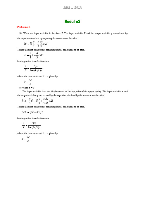
Module3Problem 3.1(a) When the input variable is the force F. The input variable F and the output variable y are related by the equation obtained by equating the moment on the stick:2.233y dy lF lkc l dt=+ Taking Laplace transforms, assuming initial conditions to be zero,433k F Y csY =+leading to the transfer function31(4)Y k F c k s=+ where the time constant τ is given by4c kτ=(b) When F = 0The input variable is x, the displacement of the top point of the upper spring. The input variable x and the output variable y are related by the equation obtained by the moment on the stick:2().2333y y dy k x l kl c l dt-=+Taking Laplace transforms, assuming initial conditions to be zero,3(24)kX k cs Y =+leading to the transfer function321(2)Y X c k s=+ where the time constant τ is given by2c kτ=Problem 3.2 P 54Determine the output of the open-loop systemG(s) =1asT+ to the inputr(t) = tSketch both input and output as functions of time, and determine the steady-state error between the input and output. Compare the result with that given by Fig3.7 . Solution :While the input r(t) = t , use Laplace transforms, Input r(s)=21sOutputc(s) = r(s) G(s) = 2(1)aTs s ⋅+ = 211T T a s s Ts ⎛⎫⎪-+⎪ ⎪+⎝⎭the time-domain response becomes c(t) = ()1t Tat aT e---Problem 3.33.3 The massless bar shown in Fig.P3.3 has been displaced a distance 0x and is subjected to a unit impulse δ in the direction shown. Find the response of the system for t>0 and sketch the result as a function of time. Confirm the steady-state response using the final-value theorem. Solution :The equation obtained by equating the force:00()kx cx t δ+=Taking Laplace transforms, assuming initial condition to be zero,K 0X +Cs 0X =1leading to the transfer function()X F s =1K Cs +=1C1K s C+The time-domain response becomesx(t)=1CC t Ke-The steady-state response using the final-value theorem:lim ()t x t →∞=0lim s →s1K Cs +1s =1K00000()()()1;11111()K t CK x x Cx t Kx X K Cs Kx Kx X C Cs K K s KKx x t eCδ-++=⇒++=--∴==⋅++-=⋅According to the final-value theorem:0001lim ()lim lim01t s s Kx sx t s X C K s K→∞→→-=⋅=⋅=+Problem 3.4 Solution:1.If the input is a unit step, then1()R s s=()()11R s C s sτ−−−→−−−→+leading to,1()(1)C s s sτ=+taking the inverse Laplace transform gives,()1tc t e τ-=-as the steady-state output is said to have been achieved once it is within 1% of the final value, we can solute “t” like this,()199%1tc t e τ-=-=⨯ (the final value is 1)hence,0.014.60546.05te t sττ-==⨯=(the time constant τ=10s) 2.the numerical value of the numerator of the transfer function doesn’t affect the answer. See this equation, If()()()1C s AG s R s sτ==+ then()(1)A C s s sτ=+giving the time-domain response()(1)tc t A e τ-=-as the final value is A, the steady-state output is achieved when,()(1)99%tc t A e A τ-=-=⨯solute the equation, t=4.605τ=46.05sthe result make no different from that above, so we said that the numerical value of the numerator of the transfer function doesn’t affect the answer.If a<1, as the time increase, the two lines won`t cross. In the steady state the output lags the input by a time by more than the time constant T.The steady error will be negative infinite.R(t)C(t)Fig 3.7 tR(t)C(t)tIf a=1, as the time increase, the two lines will be parallel. It is as same as Fig 3.7.R(t)C(t)tIf a>1, as the time increase, the two lines will cross. In the steady state the output lags the input by a time by less than the time constant T.The steady error will be positive infinite.Problem 3.5 Solution: R(s)=261s s +, Y(s)=26(51)s s s +⋅+=229614551s s s -+++ /5()62929t y t t e -∴=-+so the steady-state error is 29(-30). To conform the result:5lim ()lim(62929);tt t y t t -→∞→∞=-+=∞6lim ()lim ()lim ()lim(51)t s s s s y t y s Y s s s →∞→→→+====∞+.20lim ()lim ()lim [()()]161lim [()1]()lim (1)()5130ss t s s s s e e t S E S S Y S R S S G S R S S S S S→∞→→→→==⋅=⋅-=⋅-=⋅-⋅++=- Therefore, the solution is basically correct.Problem 3.623y y x +=since input is of constant amplitude and variable frequency , it can be represented as:j tX eA ω=as we know ,the output should be a sinusoidal signal with the same frequency of the input ,it can also be represented as:R(t)C(t)t0j t y y e ω=hence23j tj tj tj yyeeeA ωωωω+=00132j y Aω=+y2t a n3w ϕ=- Its DC(w→0) value is 003Ay ω==Requirement12w yy==0123A =⨯→32w = while phase lag of the input:1tan 14πϕ-=-=-Problem 3.7One definition of the bandwidth of a system is the frequency range over which the amplitude of the output signal is greater than 70% of the input signal amplitude when a system is subjected to a harmonic input. Find a relationship between the bandwidth and the time constant of a first-order system. What is the phase angle at the bandwidth frequency ? Solution :From the equation 3.4100.7A r =≥ (1)and ω≥0 (2)so 1.020ωτ≤≤so the bandwidth 1.02B ωτ=from the equation 3.43 the phase angle110tan tan 1.024c πωτ--∠=-=-=Problem 3.8 3.8 SolutionAccording to generalized transfer function of First-Order Feedback Systems11C KG K RKGHK sτ==+++the steady state of the output of this system is 2.5V .∴if s →0, 2.51104C R→=. From this ,we can get the value of K, that is 13K =.Since we know that the step input is 10V , taking Laplace transforms,the input is 10S .Then the output is followed1103()113C s S s τ=⨯++Taking reverse Laplace transforms,4/4332.5 2.5 2.5(1)t t C e eττ--=-=-From the figure, we can see that when the time reached 3s,the value of output is 86% of the steady state. So we can know34823(2)*4393τττ-=-⇒-=-⇒=, 4/3310.8642t t e ττ-=-=⇒=The transfer function is3128s +146s+Let 12+8s=0, we can get the pole, that is1.5s =-2/3-Problem 3.9 Page 55 Solution:The transfer function can be represented,()()()()()()()o o m i m i v s v s v s G s v s v s v s ==⋅ While,()1()111//()()11//o m m i v s v s sRCR v s sC sC v s R R sC sC =+⎛⎫+ ⎪⎝⎭=⎡⎤⎛⎫++ ⎪⎢⎥⎝⎭⎣⎦21()13()G s sRC sRC =++ And the reason:the second simple lag compensation network can be regarded as the load of the first one, and according to Load Effect , the load affects the primary relationship; so the transfer function of the combination doesn’t equal the product of the two individual lag transfer functionModule4Problem4.14.1The closed-loop transfer function is10(6)102(6)101610S S S S C RS s +++++==Comparing with the generalized second-order system,we getProblem4.34.3Considering the spring rise x and the mass rise y. Using Newton’s second law of motion..()()d x y m y K x y cdt-=-+ Taking Laplace transforms, assuming zero initial conditions2mYs KX KY csX csY =-+-resulting in the transfer funcition where2Y cs KX ms cs K+=++And51.26*10c ζ== Problem4.4Solution:261n n d W EW E W W =====2121212K C K S S K R S S K S S ∙+==+++∙+ Comparing the closed-loop transfer function with the generalized form,2222n n nCR s s ωξωω=++ it is seen that2n K ω=And that22n ξω= ;ξ=The percentage overshoot is therefore100PO=100=Where10%PO ≤When solved, gives 1.2K ≤(2.86)When K takes the value 1.2, the poles of the system are given by22 1.20s s ++=Which gives10.45s j =-±±s=-1 1.36jReProblem4.54.5 A unity-feedback control system has the forward-path transfer functionG (s) =10)S(s K+Find the closed-loop transfer function, and develop expressions for the damping ratio And damped natural frequency in term of K Plot the closed-loop poles on the complex Plane for K = 0,10,25,50,100.For each value of K calculate the corresponding damping ratio and damped natural frequency. What conclusions can you draw from the plot?Solution: Substitute G(s)=(10)K s s + into the feedback formula : Φ(s)=()1()G S HG S +.And in unit feedback systemH=1.Result in: Φ(s)=210Ks s K++So the damped natural frequencyn ω,damping ratio ζ.The characteristic equation is 2s +10S+K=0.When K ≤25,s=5-±While K>25,s=5-±The value ofn ω and ζ corresponding to K are listed as follows.K 0 10 25 50 100Pole 1 1S 0 5-+ -5 -5+5i 5-+Pole 2 2S -10 5- -5 -5-5i 5--n ω 05 10ζ ∞10.5Plot the complex plane for each value of K:We can conclude from the plot.When k ≤25,poles distribute on the real axis. The smaller value of K is, the farther poles is away from point –5. The larger value of K is, the nearer poles is away from point –5.When k>25,poles distribute away from the real axis. The smaller value of K is, the further (nearer) poles is away from point –5. The larger value of K is, the nearer (farther) poles is away from point –5.And all the poles distribute on a line parallels imaginary axis, intersect real axis on the pole –5.Problem4.61tb bR L C b ov dv i i i i v dt CR Ldt=++=++⎰Taking Laplace transforms, assuming zero initial conditions, reduces this equation to011b I Cs V R Ls ⎛⎫=++ ⎪⎝⎭20b V RLs I Ls R RLCs =++Since the input is a constant current i 0, so01I s=then,()2b RLC s V Ls R RLCs ==++Applying the final-value theorem yields()()0lim lim 0t s c t sC s →∞→==indicating that the steady-state voltage across the capacitor C eventually reaches the zero ,resulting in full error.Problem4.7 4.7 Prove that for an underdamped second-order system subject to a step input, the percentageovershoot above the steady-state output is a function only of the damping ratio .Fig .4.7SolutionThe output can be given by222222()(2)21()(1)n n n n n n C s s s s s s s ωζωωζωζωωζ=+++=-++- (1) the damped natural frequencyd ω can be defined asd ω=ω (2)substituting above results in22221()()()n n n d n d s C s s s s ζωζωζωωζωω+=--++++ (3) taking the inverse transform yields()1)tan n t d c t t where ζωωφφ-=+=(4)the maximum output is()1sin()n t p d p p d e c t t t ζωωφππω-=-+==(5)so the maximum is()1p c t eπζ-=+the percentage overshoot is therefore100PO eπζ-=Problem4.8 Solution to 4.8:Considering the mass m displaced a distance x from its equilibrium position, the free-body diagram of the mass will be as shown as follows.aUsing Newton’s second law of motion,22p k x c x m x m x c x k x p--=++=Taking Laplace transforms, assuming zero initial conditions,2(2)X ms cs k P ++=results in the transfer function2/(1/)/((/)2/)X P m s c m s k m =++ 2(2/)(2/)((/)2/)k k m s c m s k m =++As we see2(2)X m s c s k P ++= As P is constantSo X ∝212ms cs k ++ . When 56.25102cs m-=-=-⨯()25min210mscs k ++=4max5100.110X == This is a second-order transfer function where22/n k m ω=and/2/n c w mc m ζ==The damped natural frequency is given byd ωω===Using the given data,0.2236n ω===42.795010ζ-==⨯0.223100.2236d ω==With these data we can draw a picture14.0501160004.673600p de s e T T πωτζωτ======2222112/1222()2sin (sin cos )0tan 7.030.02n n pp dd n dd n ntd dt t t n d p d d p ddd p p p nX k m c k P ms cs k k m s s s m m cm p x e tm p x e t tm t t x m ζωζωωωζωωωωζζωωωζωωωωωωωζω--===⋅=⋅++++++====∴==-+=∴=⇒=⇒=其中Problem4.10 4.10 solution:The system is similar to the one in the book on PAGE 58 to PAGE 63. The difference is the connection of the spring. So the transfer function is2222l n d n n w s w s w θθζ=++222(),;pa m ld a m p m l m l l m mm l lk k k N RJs RCs R k k N k J N J J C N c c N N N θθωθωθ=+++=+=+===n w =damping ratioζ=But the value of J is different, because there is a spring connected.122s m J J J J N N '=++Because of final-value theorem,2l nd w θθζ=Module5Problem5.45.4 The closed-loop transfer function of the system may be written as2221010(1)610101*********C RK K KS S K KS S K S S +++==+++++++ The closed-loop poles are the solutions of the characteristic equation3n S W ==-±= 26E ==In order to study the stability of the system, the behavior of the closed-loop poles when thegain K increases from zero to infinte will be observed. So when12K =10E =3S =-210K =110E =3S =-± 320K = 70E =3S =-±双击下面可以看到原图ReProblem5.5SolutionThe closed-loop transfer function is2222(1)1(1)KC K KsKR s K as s aKs Kass===+++++∙+Comparing the closed-loop transfer function with the generalized form, 2222nn nCR s sωξωω=++Leading to2nωξ==The percentage overshoot is therefore10040%PO==Producing the result0.869ξ=(0.28)And the peak time4PT s==Leading to1.586nω=(0.82)Problem5.75.7 Prove that the rise time T r of a second-order system with a unit step input is given byT r = d ω1tan -1n d ζωω = d ω1tan -1dωζ21--Plot the rise against the damping ratio.Solution:According to (4.33):c(t)=1-(cos )n t d d e t t ζωωω-. 4.33When t=r T ,c(t)=1.substitue c(t)= 1 into (4.33) Producing the resultr T =d ω1tan -1n d ζωω = d ω1tanPlot the rise time against the damping ratio:Problem5.9Solution to 5.9:As we know that the system is the open-loop transfer function of a unity-feedback control system. So ()()GH S G S = Given as()()()425KGH s s s =-+The close-loop transfer function of the system may be written as()()()()()41254G s C Ks R GH s s s K==+-++ The characteristic equation is()()2254034100s s K s s K -++=⇒++-=According to the Routh’s method, the Routh’s array must be formed as follow20141030410s K s s K --For there is no closed-loop poles to the right of the imaginary axis4100 2.5K K -≥⇒≥Given that 0.5ζ=4.75n K ωζ==⇒= When K=0, the root are s=+2,-5According to the characteristic equation, the solutions are32s =-±while 3.0625K ≤, we have one or two solutions, all are integral number.Or we will have solutions with imaginary number. So we can drawProblem5.10 5.10 solution:0.62/n w rad sζ==according to()11)2n w t d c w t ζφ-=+=1.2sin(1.6)0.4t e t φ-⋅+= 4tan 3φ=finally, t is delay time:1.23t s ≈(0.67)Module6Problem 6.3First we assume the disturbance D to be zero:e R C =-1011C K e s s=⋅⋅⋅+ Hence:(1)10(1)e s s R K s s +=++ Then we set the input R to be zero:10()(1)C K e D e s s =⋅+⋅=-+ ⇒ 1010(1)e D K s s =-++Adding these two results together:(1)1010(1)10(1)s s e R D K s s K s s +=⋅-⋅++++21()R s s= ; 1()D s s = ∴222110910(1)10(1)100(1)s s e Ks s s Ks s s s s s +-=-=++++++ the steady-state error:232200099lim lim lim 0.09100100ss s s s s s s e s e s s s s s →→→--=⋅===-++++Problem 6.4Determine the disturbance rejection ratio(DRR) for the system shown in Fig P.6.4+fig.P.6.4 solution :from the diagram we can know :0.210.05mv K RK c === so we can get that()0.21115()0.05v m m OL n CL K K DRR cR ωω∆⨯==+=+=∆210.10.050.050.025s s =++, so c=0.025, DRR=9Problem 6.5 6.5 SolutionFor the purposes of determining the steady-state error of the system, we should get to know the effect of the input and the disturbance along when the other will be assumed to be zero.First to simplify the block diagram to the following patter:Allowing the transfer function from the input to the output position to be written as01220220d Js s θθ=++ 012222020240*220220(220)dJs s Js s s Js s sθθ===++++++ According to the equation E=R-C:022*******(2)()lim[()()]lim[(1)]lim 0.2220220ssr d s s s Js e s s s s Js s Js s δδδθθ→→→+=-=-==++++问题;1. 系统型为2,对于阶跃输入,稳态误差为0.2. 终值定理写的不对。
自动控制原理第三版

自动控制原理第三版自动控制原理(第三版)1. 引言自动控制是一门研究如何实现系统的稳定和性能优化的学科。
它广泛应用于工业、交通、能源等领域,为提高生产效率、资源利用率和安全性起到重要作用。
2. 控制系统基础2.1 系统建模系统建模是控制系统设计的基础。
它可以将实际系统抽象为数学模型,以便进行分析和设计控制策略。
2.2 信号与系统信号与系统是理解控制系统行为的重要工具。
常用的信号类型有连续时间信号和离散时间信号,而系统可以通过输入输出关系进行描述。
3. 线性控制系统3.1 常见控制器比例控制器、积分控制器和微分控制器是常见的线性控制器。
它们根据系统误差的不同类型,分别进行修正和控制。
3.2 闭环控制系统闭环控制系统通过测量系统输出,并与期望输出进行对比,从而实现误差修正。
闭环控制系统更稳定,但需要合适的设计方案。
4. 非线性控制系统4.1 反馈线性化反馈线性化是一种处理非线性系统的方法。
它通过改变系统输入和输出,使得系统在某种条件下可以近似为线性系统进行控制。
4.2 多变量控制系统多变量控制系统涉及多个输入和输出变量的控制。
它需要考虑各个变量之间的相互影响,以及设计相应的控制策略。
5. 齐次与非齐次系统5.1 齐次系统齐次系统是其输入与输出之间的关系满足齐次性的系统。
它的特点是具有线性、时不变、可加性等性质。
5.2 非齐次系统非齐次系统是不满足齐次性的系统。
它可能由于扰动或非线性因素而引起输出与输入之间的差异。
6. 状态空间法6.1 状态空间模型状态空间模型是一种用状态变量表示系统状态的方法。
它更直观地描述了系统的动态行为,并便于进行分析和控制。
6.2 状态反馈控制状态反馈控制通过测量系统状态,并与期望状态进行对比,从而实现误差修正。
它在系统稳定性和性能优化方面具有重要意义。
7. 控制系统设计7.1 控制系统设计步骤控制系统设计通常包括建模、分析、控制器设计和仿真等步骤。
每一步都需要合理和有效地完成,以确保设计的最终效果。
自动控制原理第3章习题解答

(2) k (t ) = 5t + 10 sin( 4t + 45 )
0
(3) k (t ) = 0.1(1 − e 解: (1) Φ ( s ) =
−t / 3
)
0.0125 s + 1.25
1
胡寿松自动控制原理习题解答第三章
(2) k (t ) = 5t + 10 sin 4t cos 45 + 10 cos 4t sin 45
3s 4 + 10s 3 + 5s 2 + s + 2 = 0
试用劳思稳定判据和赫尔维茨判据确定系统的稳定性。 解: 列劳思表如下:
s4 s3 s2 s1 s0
3 5 2 10 1 47 2 10 1530 0 − 47 2
由劳思表可以得到该系统不稳定。 3-12 已知系统特征方程如下,试求系统在 s 右半平面的根数及虚根值。 (1)
2ξω n = 70
ξ=
7 2 6
根据(3-17)
h(t ) = 1 +
e − t / T1 e − t / T12 + T2 / T1 − 1 T1 / T2 − 1
解:根据公式(3-17)
3
胡寿松自动控制原理习题解答第三章
自动控制原理 习题答案分析第三章 华南理工版
100% 16.3%
3 1 1 1.5秒 , ts 或 ln 1.57秒 2 ςωn ςωn Δ 1 ς
自动控制原理习题分析第三章3-11(1)
已知单位反馈系统的闭 环传递函数 : 7.6(s 2.1) Φ(s) .试估算σ%和t s 2 (s 8)(s 2)(s s 1)
已 知 随 动 系 统 如 图 .当 8时 , 求 : K 试 (1)系 统 的 特 征 参 量和 ω ; ς n (2)系 统 的 动 态 性 能 标 σ %和 t . 指 s
自动控制原理习题分析第三章3-8
8 G( s ) ; s(0.5s 1)
2 G(s) 8 16 ωn Φ(s) 2 2 2 1 G(s) s(0.5s 1) 8 s 2s 16 s 2ςωns ωn 2 ωn 16 ωn 4;2ςωn 2 ςωn 1,ς 0.25;
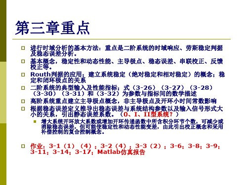
3-3 判断使系统稳定的K的范围:放大系数可否为复数? 3-11(2) 过阻尼系统,求ts(用欠阻尼公式?) 3-11(1) 主导极点分析(偶极子,模比(wn)>5) 计算ts的时候,需指明Δ 是5%还是2% 3-14 计算稳态误差 3-17 计算复合控制
自动控制原理习题分析第三章3-1(1)
已知单位反馈系统的开 传递函数, 环 试用劳思判据判断系统 稳定性. 的 50 G(s) ; s(s 1)(s 5)
ς 0.5 0.0163888 0.0211111 ;式 中: ωn 1 s8 s2
自动控制原理习题分析第三章3-11(1)
c(t) 0.9975(1 1.1547e0 . 5 t sin(0.866t 60)) 0.1139392e
自动控制原理第三章习题答案

第三章习题答案名词解释1.超调量:系统响应的最大值与稳态值之差除以稳态值。
定义为)()(max ∞∞-=c c c σ 2.开环传递函数中含有2个积分因子的系统称为II 型系统。
3.单位阶跃响应达到第一个峰值所需时间。
4.指响应达到并保持在终值5%内所需要的最短时间。
5. 稳态误差:反馈系统误差信号e(t) 的稳态分量(1分),记作e ss (t)。
6.开环传递函数中不含有积分因子的系统。
7.上升时间:○1响应从终值10%上升到终值90%所需的时间;或○2响应从零第一次上升到终值所需的时间。
简答1. 在实际控制系统中,总存在干扰信号。
1) 时域分析:干扰信号变化速率快,而微分器是对输入信号进行求导,因此干扰信号通过微分器之后,会产生较大的输出;2) 频域分析:干扰信号为高频信号,微分器具有较高的高频增益,因此干扰信号易被放大。
这就是实际控制系统中较少使用纯微分器的原因。
2.系统稳定的充分条件为:劳斯阵列第一列所有元素不变号。
若变号,则改变次数代表正实部特征根的数目。
3.二阶临界阻尼系统特征根在负实轴上有两个相等的实根,其单位阶跃响应为单调递增曲线,最后收敛到一个稳态值。
4. 闭环特征根严格位于s 左半平面;或具有负实部的闭环特征根。
5.欠阻尼状态下特征根为一对具有负实部的共轭复数,单位阶跃响应是一个振荡衰减的曲线,最后收敛到一个稳态值。
6.阻尼小于-1的系统,特征根位于正实轴上,单位阶跃响应是一个单调发散的曲线。
7. 无阻尼状态下特征根为一对虚根,响应为等幅振荡过程,永不衰减。
8.图4(a)所示系统稳定,而图4(b)所示系统不稳定。
原因是图4(b)所示系统的小球收到干扰后将不能恢复到原来的平衡状态。
9.不能。
原因是:两个一阶惯性环节串联后的极点为实极点;而二阶振荡环节的极点为复数极点。
计算题1. 解:r(t)=2t.v=1,系统为I 型系统k v =2,e ss =1.2.解:构造Routh 表:25:010:255:03/803/16:25203:35121:012345s s s s s s辅助方程:02552=+s 故纯虚根为:j s 52,1±=;故系统处于临界稳定状态。
自动控制原理第三章
P75 二阶系统的 结构图
20
2019/4/2
《自动控制原理》第三章
1、无阻尼情况 ( 0)
s 1 ct (t ) L [ 2 ] cos nt t 0 2 s n
等幅振 荡
特征方程有一对共轭虚根 s1,2 jn 2、欠阻尼情况 (0 1)
2019/4/2
《自动控制原理》第三章
7
三.劳斯稳定判据的应用
1、判断系统的稳定性 例: a3 s 3 a2 s 2 a1s a0 0 解:
判断稳定性。
s
3
a3 a2 a1a2 a3 a0 a2 a0
a1 a0 0
0 0
s2 s1 s
0
三阶系统稳定的充要条件是: ai
2019/4/2
瞬态ct (t ) e
ct (t )
t
T
, 稳态css (t ) 1(t )
css (t )
dc(t ) 1 e t /T dt t 0 T
c(t )
t 0
1 T
+
=
2019/4/2
《自动控制原理》第三章
18
二.一阶系统的动态性能指标
c(t )
t 3T
(1 e
t /T
)
t 3T
1 e
3T /T
0.95
T0 T 1 K0
ts 3T
ts 是一阶系统的动态性能指标。
增大系统的开环放大系数K0 会使T 减小,使ts 减小。
2019/4/2
《自动控制原理》第三章
19
第四节
二阶系统的动态性能指标
二阶标准型 或称典型二阶系 统传递函数
自动控制原理(全套课件)

自动控制原理(全套课件)一、引言自动控制原理是自动化领域的一门重要学科,它主要研究如何利用各种控制方法,使系统在受到扰动时,能够自动地、准确地、快速地恢复到平衡状态。
本课件将详细介绍自动控制的基本概念、控制系统的类型、数学模型、稳定性分析、控制器设计等内容,帮助学员全面掌握自动控制原理的基本理论和方法。
二、控制系统的基本概念1. 自动控制自动控制是指在没有人直接参与的情况下,利用控制器使被控对象按照预定规律运行的过程。
自动控制的核心在于控制器的设计,它能够根据被控对象的运行状态,自动地调整控制量,使系统达到预期的性能指标。
2. 控制系统控制系统是由被控对象、控制器、传感器和执行器等组成的闭环系统。
被控对象是指需要控制的物理过程或设备,控制器负责产生控制信号,传感器用于测量被控对象的运行状态,执行器则根据控制信号对被控对象进行操作。
三、控制系统的类型1. 按控制方式分类(1)开环控制系统:控制器不依赖于被控对象的运行状态,直接产生控制信号。
开环控制系统简单,但抗干扰能力较差。
(2)闭环控制系统:控制器依赖于被控对象的运行状态,通过反馈环节产生控制信号。
闭环控制系统抗干扰能力强,但设计复杂。
2. 按控制信号分类(1)连续控制系统:控制信号是连续变化的,如模拟控制系统。
(2)离散控制系统:控制信号是离散变化的,如数字控制系统。
四、控制系统的数学模型1. 微分方程模型微分方程模型是描述控制系统动态性能的一种数学模型,它反映了系统输入、输出之间的微分关系。
通过求解微分方程,可以得到系统在不同时刻的输出值。
2. 传递函数模型传递函数模型是描述控制系统稳态性能的一种数学模型,它反映了系统输入、输出之间的频率响应关系。
传递函数可以通过拉普拉斯变换得到,它是控制系统分析、设计的重要工具。
五、控制系统的稳定性分析1. 李雅普诺夫稳定性分析:通过构造李雅普诺夫函数,分析系统的稳定性。
2. 根轨迹分析:通过分析系统特征根的轨迹,判断系统的稳定性。
自动控制原理第三章3_劳斯公式

j1 j1 j
23
2
若代数方程有对称于虚轴的实根 或共轭复根,则一定在劳斯表的 第一列有变号,并可由辅助方程 求出
分析系统参数变化对稳定性的影响 利用劳斯稳定性判据还可以讨论个别参数对稳定性的影响, 从而求得这些参数的取值范围。若讨论的参数为开环放大系数K, Kp 则使系统稳定的最大K称为临界放大系数 。 [例3-7]已知系统的结构图,试确定系统的临界放大系数。
稳定的基本概念: 设系统处于某一起始的平衡状态。在外作用的影响下,离 开了该平衡状态。当外作用消失后,如果经过足够长的时间它 能回复到原来的起始平衡状态,则称这样的系统为稳定的系统 。 否则为不稳定的系统。
稳定的充要条件和属性
线性系统稳定的充要条件: 系统特征方程的根(即传递函数的极点)全为负实数或具 有负实部的共轭复根。或者说,特征方程的根应全部位于s平面 的左半部。
3
要使系统稳定,必须 k 0 ①系数皆大于0, ②劳斯阵第一列皆大于0 120 k 0 k 120 有 8 0 k 120 k 0
所以,临界放大系数 k p 120 确定系统的相对稳定性(稳定裕度) 利用劳斯和胡尔维茨稳定性判据确定的是系统稳定或不稳 定,即绝对稳定性。在实际系统中,往往需要知道系统离临界 稳定有多少裕量,这就是相对稳定性或稳定裕量问题。
2 2 5 4 3 2 ( s 4 )( s 25 )( s 2 ) s 2 s 24 s 48 s 25s 50 例如: 1
2 (s 2 4)
[处理办法]:可将不为零的最后一行的系数组成辅助方程,对 此辅助方程式对s求导所得方程的系数代替全零的行。大小相等, 位置径向相反的根可以通过求解辅助方程得到。辅助方程应为 偶次数的。