统计模拟与R第一讲
R语言数据分析与统计建模入门指南

R语言数据分析与统计建模入门指南Chapter 1: Introduction to R Programming LanguageR is a powerful programming language and software environment for statistical computing and graphics. It provides a wide range of statistical and graphical techniques, making it a popular choice for data analysis and statistical modeling. In this chapter, we will introduce the basics of R programming language and its features.1.1 Installing and Setting up RTo get started with R, you need to install it on your computer. R is available for Windows, macOS, and Linux operating systems. Once installed, you can launch the R console or RStudio, which is an integrated development environment (IDE) for R. RStudio provides a user-friendly interface for writing code, managing files, and visualizing data.1.2 Basic R SyntaxR uses a combination of functions, operators, and variables to perform calculations and manipulate data. The basic syntax of R is similar to other programming languages. For example, you can use the assignment operator ( <- ) to assign a value to a variable, or use arithmetic operators (+, -, *, /) to perform calculations.1.3 Data Types in RR supports various data types, including numeric, character, logical, and complex. Numeric data types represent real numbers, character data types store text, logical data types are used to represent logical values (TRUE or FALSE), and complex data types store complex numbers.1.4 Data Structures in RR provides several built-in data structures for storing and organizing data. These include vectors, matrices, data frames, and lists. Vectors are one-dimensional arrays that can store multiple values of the same data type. Matrices are two-dimensional arrays with rows and columns. Data frames are similar to tables in a relational database, and lists can store different types of objects.Chapter 2: Data Import and Manipulation in RIn this chapter, we will focus on how to import data from different file formats into R and perform data manipulation tasks.2.1 Importing Data from CSV FilesCSV (Comma-Separated Values) files are a common format for storing tabular data. R provides functions like read.csv() and read.csv2() to import data from CSV files. These functions automatically detect the delimiters and create data frames in R.2.2 Working with Data FramesData frames are a popular data structure in R. They are similar to tables in a database, with rows and columns. In this section, we will explore various operations that can be performed on data frames, such as subsetting, merging, and sorting.2.3 Data Cleaning and PreprocessingBefore starting any analysis, it is essential to clean and preprocess the data. R offers a wide range of functions and packages for data cleaning, such as removing missing values, handling outliers, and transforming variables. We will explore some commonly used techniques in this section.Chapter 3: Exploratory Data AnalysisExploratory Data Analysis (EDA) is a crucial step in data analysis. It involves summarizing and visualizing the main characteristics of the data. In this chapter, we will learn different techniques to explore and visualize the data using R.3.1 Descriptive StatisticsDescriptive statistics provide summary measures that describe the central tendency, variability, and distribution of the data. R provides functions like mean(), median(), and sd() to calculate these statistics. We will also cover graphical techniques, such as histograms and box plots.3.2 Data VisualizationR offers a rich set of packages for data visualization. We will explore popular packages like ggplot2, which provides a flexible and powerful grammar for creating elegant graphics. We will cover different types of plots, such as scatter plots, bar plots, and density plots.Chapter 4: Statistical Modeling in RStatistical modeling involves building mathematical models to describe and analyze relationships between variables. In this chapter, we will cover some fundamental statistical modeling techniques using R.4.1 Regression AnalysisRegression analysis is a statistical technique used to model the relationship between a dependent variable and one or more independent variables. R provides various functions for fitting linear regression models, such as lm() and glm(). We will learn how to interpret the regression models and assess their goodness of fit.4.2 Hypothesis TestingHypothesis testing is a statistical method used to make inferences about populations based on sample data. R provides functions liket.test() and prop.test() to perform hypothesis tests for means and proportions, respectively. We will discuss the steps involved in hypothesis testing and interpret the results.4.3 ANOVA and Chi-Square TestANOVA (Analysis of Variance) and Chi-Square tests are commonly used statistical tests in various research areas. R provides functions like aov() and chisq.test() to perform these tests. We will learn how to conduct ANOVA tests for comparing means across groups and Chi-Square tests for testing associations between categorical variables.ConclusionIn this introductory guide to R programming language for data analysis and statistical modeling, we covered the basics of R syntax, data types, data structures, import/export, data manipulation, exploratory data analysis, and statistical modeling techniques. R offers a wide range of capabilities for analyzing and visualizing data, making it an essential tool for data scientists and statisticians. With practice and further exploration of R's vast library of packages, you can deepen your knowledge and become proficient in using R for data analysis and statistical modeling.。
统计建模与R软件课后问题详解
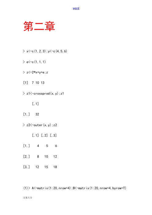
第二章> x<-c(1,2,3);y<-c(4,5,6)> e<-c(1,1,1)> z<-2*x+y+e;z[1] 7 10 13> z1<-crossprod(x,y);z1[,1][1,] 32> z2<-outer(x,y);z2[,1] [,2] [,3][1,] 4 5 6[2,] 8 10 12[3,] 12 15 18(1)> A<-matrix(1:20,nrow=4);B<-matrix(1:20,nrow=4,byrow=T)> C<-A+B;C(2)> D<-A%*%B;D(3)> E<-A*B;E(4)> F<-A[1:3,1:3](5)> G<-B[,-3]> x<-c(rep(1,5),rep(2,3),rep(3,4),rep(4,2));x> H<-matrix(nrow=5,ncol=5)> for (i in 1:5)+ for(j in 1:5)+ H[i,j]<-1/(i+j-1)〔1〕> det(H)〔2〕> solve(H)〔3〕> eigen(H)> studentdata<-data.frame(某某=c('X三','李四','王五','赵六','丁一')+ ,性别=c('女','男','女','男','女'),年龄=c('14','15','16','14','15'),+ 身高=c('156','165','157','162','159'),体重=c('42','49','41.5','52','45.5'))> write.table(studentdata,file='student.txt')> write.csv(studentdata,file='student.csv')count<-function(n){if (n<=0)print('要求输入一个正整数')else{repeat{if (n%%2==0)n<-n/2elsen<-(3*n+1)if(n==1)break}print('运算成功')}}第三章首先将数据录入为x。
统计模拟

11
Monte Carlo方法简史
2、1930年,Enrico Fermi利用Monte Carlo方法研究中 子的扩散,并设计了一个Monte Carlo机械装臵, Fermiac,用于计算核反应堆的临界状态 3、Von Neumann是Monte Carlo方法的正式奠基者,他与 Stanislaw Ulam合作建立了概率密度函数、反累积分布 函数的数学基础,以及伪随机数产生器。在这些工作中 ,Stanislaw Ulam意识到了数字计算机的重要性
合作起源于Manhattan工程:利用 ENIAC(Electronic Numerical Integrator and Computer)计算产额 Nhomakorabea
4、随着计算机和统计技术的快速发展,Monte Carlo方 法不断丰富、应用也越来越广泛
13
Monte Carlo模拟的应用:
自然现象的模拟: 宇宙射线在地球大气中的传输过程; 高能物理实验中的核相互作用过程; 实验探测器的模拟 数值分析: 利用Monte Carlo方法求积分 金融工程: 股票期权的模拟定价 离散事件的模拟 ……
例子: >3+5 >3-5 >3/5 >3^5 >x=5 >?plot >help(plot)
32
向量
向量是R中最为基本的类型 一个向量中元素的类型必须相同,包括
统计模拟
主讲教师:刘洪伟 E-mail: liuhungwei@
1
目录
第一章 第二章 第三章 第四章 第五章 第六章 第七章 第八章
统计建模与R软件假设检验习题答案

04 习题答案解析
习题一答案解析
答案:D
解析:根据题目描述,A、B、C三个选项都是描述数据特征的,而D选项是描述数据来源的,与题目 要求的“数据特征”不符。
习题二答案解析
答案:B
解析:根据题目要求,需要选择一个假设检验的方法。A选项是参数检验,适用于总体分布已知的情况;B选项是非参数检验 ,适用于总体分布未知或不符合正态分布的情况;C选项是回归分析,用于研究变量之间的关系;D选项是聚类分析,用于数 据的分类。根据题目描述,由于总体分布未知且不符合正态分布,所以选择B选项。
模型评估
01
02
03
交叉验证
将数据集分成训练集和测 试集,使用训练集训练模 型,在测试集上评估模型 的性能。
均方误差
衡量预测值与实际值之间 的误差,越小越好。
准确率
衡量分类模型正确预测的 比例,越高越好。
02 R软件基础
R软件介绍
总结词
R软件是一种开源的统计计算和图形绘制软件,广泛应用于数据分析和统计建模 。
解析:根据题目要求,需要选择一个统计量 来描述数据的集中趋势。A选项是平均数, 是最常用的描述集中趋势的统计量;B选项 是中位数,描述数据的中位数位置;C选项 是众数,描述数据中出现次数最多的数;D 选项是标准差,描述数据的离散程度。根据
题目要求,选择A选项。
习题五答案解析
答案:C
解析:根据题目要求,需要选择一个统计量来检验两 个样本是否来自同一个总体。A选项是t检验,适用于 两个正态分布的总体;B选项是卡方检验,适用于分 类数据的比较;C选项是F检验,适用于两个总体方差 的比较;D选项是z检验,适用于总体比例的比较。根 据题目要求,选择C选项。
假设检验的优缺点
统计建模与R软件课程报告

统计建模与R软件课程报告对某地区农业生态经济的发展状况作主成分分析主成分分析的主要目的是希望用较少的变量去解释原来资料中的大部分变异,将我们手中许多相关性很高的变量转化成彼此相关独立或不相关的变量。
通常是选出比原始变量个数少,又能解释大部分资料中的变异的几个新变量,即所谓主成分,并用以解释资料的综合性指标。
也就是说,主成分分析实际上是一种降维方法。
关键词:主成分分析相关矩阵相关R函数1 绪论 (2)1.1主成分方法简介 (2)2总体主成分 (2)2.1主成分的定义与导出 (2)2.2主成分的性质 (3)2.3从相关矩阵出发求主成分 (5)2.4相关的R函数 (6)3数据模拟 (7)4结论及对该模型的评价 (12)参考文献 (12)1.1主成分方法简介主成分分析(principal component analysis )是将多个指标化为少数几个 综合指标的一种统计分析方法,由Pearson( 1901)提出,后来被Hotelling ( 1933) 发展了。
主成分分析是一种通过降维技术把多个变量化成少数几个主成分的方法。
这些主成分能够反映原始变量的绝大部分信息,它们通常表示为原始变量的线性 组合。
主成分分析也称主分量分析, 旨在利用降维的思想,把多指标转化为少数几个综合指标。
在实证问题研究中,为了全面、系统地分析问题,我们必须考虑众多影响因素。
这些涉及的 因素一般称为指标,在多元统计分析中也称为变量。
因为每个变量都在不同程度上反映了所研究问题的某些信息,并且指标之间彼此有一定的相关性,因而所得的统计数据反映的信息在一定程度上有重叠。
在用统计方法研究多变量问题时,变量太多会增加计算量和增加分析 问题的复杂性,人们希望在进行定量分析的过程中,涉及的变量较少,得到的信息量较多。
主成分分析正是适应这一要求产生的,是解决这类题的理想工具。
2总体主成分2.1主成分的定义与导出易见var( ZJ 二 a TZa i , i=1,2,,p,我们希望乙的方差达到最大,即a 1是约束优化问题max a T las.ta T a = 11绪论设x 是p 维随机变量,并假设艺二var(X )。
统计建模与R软件课程报告

统计建模与R软件课程报告Document serial number【UU89WT-UU98YT-UU8CB-UUUT-UUT108】统计建模与R软件课程报告对某地区农业生态经济的发展状况作主成分分析摘要主成分分析的主要目的是希望用较少的变量去解释原来资料中的大部分变异,将我们手中许多相关性很高的变量转化成彼此相关独立或不相关的变量。
通常是选出比原始变量个数少,又能解释大部分资料中的变异的几个新变量,即所谓主成分,并用以解释资料的综合性指标。
也就是说,主成分分析实际上是一种降维方法。
关键词:主成分分析相关矩阵相关R函数目录1 绪论主成分方法简介主成分分析(principal component analysis)是将多个指标化为少数几个综合指标的一种统计分析方法,由Pearson(1901)提出,后来被Hotelling(1933)发展了。
主成分分析是一种通过降维技术把多个变量化成少数几个主成分的方法。
这些主成分能够反映原始变量的绝大部分信息,它们通常表示为原始变量的线性组合。
主成分分析也称主分量分析,旨在利用降维的思想,把多指标转化为少数几个综合指标。
在实证问题研究中,为了全面、系统地分析问题,我们必须考虑众多影响因素。
这些涉及的因素一般称为指标,在多元统计分析中也称为变量。
因为每个变量都在不同程度上反映了所研究问题的某些信息,并且指标之间彼此有一定的相关性,因而所得的统计数据反映的信息在一定程度上有重叠。
在用统计方法研究多变量问题时,变量太多会增加计算量和增加分析问题的复杂性,人们希望在进行定量分析的过程中,涉及的变量较少,得到的信息量较多。
主成分分析正是适应这一要求产生的,是解决这类题的理想工具。
2总体主成分主成分的定义与导出设Χ是p变换T pp Z ⎪⎪=⎩⎭aX()易见()()()成分。
主成分的性质关于主成分有如下性质:(1)主成分的均值和协方差阵。
记由于() 所以有(2)主成分的总方差 由于所以pp方差之和。
R语言统计模拟

只要产生服从(0,1)均匀分布的随机变量x,然后用g作用一下,
再就平均值就可以了
o > integ <- function(h, a, b, n){ x <- runif(n); sum((b-a)*h(a+(b-a)*x))/n; }
例如要求 2 exx2 dx, 利用上述integ函数求解, 2
例如要求 exdx,利用上述integ函数求解, 0
只需要令h(x) ex
• > h <- function(x){ exp(-x);}
• > integ(h, 10000);
o 随机模拟最基本的需要是产生伪随机数,R中已提供了大多数 常用分布的伪随机数函数,可以返回一个伪随机数序列向量。
o 产生伪随机数序列是不重复的,实际上,R在产生伪随机数时从 一个种子出发,不断迭代更新种子,所以产生若干随机数后内部 的随机数种子就已经改变了。有时我们需要模拟结果是可重复的, 这只要我们保存当前的随机数种子,然后在每次产生伪随机数序 列之前把随机数种子置为保存值即可:
随机模拟的基本思想:假设我们有个区域R大小已知,在这个 区域中有一个不规则的区域M(其面积不能通过公式直接计算),请 问如何求M的面积?
R M
方法: Ø1) 把这个不规则的区域M划分成很多个小小的规则的区域,用规则小区域的面积总 和来近似逼近M的面积; Ø2) 抓一把黄豆,均匀地铺在R上,数一数R里面的黄豆数,记为S。再数一数M里的黄 豆数,记为S1,则M的近似面积为S1/S。----这就是采样的方法。
另一种求定积分的方法
根据大数定律:1
n
n i 1
g(Xi)
E(g(X
))
1
b h(t)dt
统计建模与R语言PPT课件

+
sub = G == i)
+ res.mat[i, ] <- residuals(gene.aov)
+ coef.mat[i, ] <- coef(gene.aov)
+}
或
>for(i in 1:1522)
7 3 7 10
第4页/共23页
• 向量的下标(index)与向量子集(元素)的提取 • 正的下标 提取向量中对应的元素 • 负的下标 去掉向量中对应的元素 • 逻辑运算 提出向量中元素的值满足条件的元素 注:R中向量的下标从1开始,这与通常的统计或数学软件一致而象C语言等 计算机高级语言的向量下标则从0开始!
> coef.mat = matrix(0, 1522, 4, byrow = TRUE)
> for(i in 1:1522) {
+ gene.aov = aov(Intensity ~ A + T + A * T,
+
sub = G == i)
+
res.mat[i, ] = residuals(gene.aov) # 保存ANOVA分
> ybar = data.frame(A = factor(a), G = factor(g),
+
T = factor(t), Intensity = y)
> attach(ybar)
> ybar[1:10,] # 查看ybar的前10行
> res.mat = matrix(0, 1522, 8, byrow = TRUE)
>x=c(42,7,64,9)
>length(x)
- 1、下载文档前请自行甄别文档内容的完整性,平台不提供额外的编辑、内容补充、找答案等附加服务。
- 2、"仅部分预览"的文档,不可在线预览部分如存在完整性等问题,可反馈申请退款(可完整预览的文档不适用该条件!)。
- 3、如文档侵犯您的权益,请联系客服反馈,我们会尽快为您处理(人工客服工作时间:9:00-18:30)。
比如计算积分
b
g( x)dx
a
其R程序如下:
也可采用R的内置函数来 计算积分
f1=function(n,a,b,g){
X=runif(n)
integrate(g,a,b)
sum((b-a)*g(a+(ba)*X))/length(X)
}
现举一个具体的例子比较他们的结果:
2
例 估计积分
e x x2 dx
plot(c(0,1,1,0),c(0,0,1,1),xlab=" ",ylab=" ") text(0,1,labels="A",adj=c(0,0)) text(1,1,labels="B",adj=c(1.5,0.5)) text(1,0,labels="C",adj=c(0.3,-0.8)) text(0,0,labels="D",adj=c(-0.5,0.1)) points(0.5,0.5) text(0.5,0.5,labels="o",adj=c(-1,0.3)) delta_t=0.01;n=200 x=matrix(0,nrow=5,ncol=n);x[,1]=c(0,1,1,0,0) y=matrix(0,nrow=5,ncol=n);y[,1]=c(1,1,0,0,1) d=c(0,0,0,0) for(j in 1:(n-1)){
解:建立平面直角坐标系,以时间间隔 t 进行采样,在每一时刻t计算每个人在下一
时刻 t t 时的坐标。不妨假设甲追踪乙,设在时刻t,甲、乙的坐标分别为
( x1 , y1 ), ( x2 , y2 ) 甲在 t t 时刻的坐标为 ( x1 vt cos , y1 vt sin ) d ( x2 x1 )2 ( y2 y1 )2 cos x2 x1 d , sin y2 y1 d ,
00
2.用模拟方法估计 Cov(U , eU ),其中U为(0,1)均匀分布的随机变量,并与其精确值
比较.
3.令 其中
xn 3xn1 5xn2 mod(100), n 3 x1 23, x2 66
求其前14个值.
例:追逐问题,在正方形ABCD的四个顶点各有一人, 在某一时刻,四人同时出发以匀速v走向顺时针方向的 下一个人。如果他们的方向始终保持对准目标,则最终 将按螺旋状曲线汇合于中心点O.试求这种情况下每个人的 轨迹。
}
例: 的估计:
也可以用平均值法:
1
0
1 x2 dx
4
程序
Pi2=function(n){ x=runif(n) 4*sum(sqrt(1-x^2))/n }
练习:1.估计下列积分
(1) 1 eex dx 0
(2) x(1 x2 )2dx 0
1
(3)
1 e( x y)2 dxdy
1, 0 x 1, 0 y 1 f ( x, y) 0, otherwise
则 P{ X 2 Y 2 1}
4
Pi<-function(n){ set.seed(1234579) k<-0; x<-runif(n); y<-runif(n); k <- length(x[x^2+y^2 < 1]) data.frame(Pi=4*k/n)
其中a和m为给定的正整数,每个 xn 均为0,1,2,…,m-1中的一个,
xn / m 称为一个伪随机数,它近似服从(0,1)上的均匀分布。
通常为了避免随机数的重复出现,可选取m为与计算机字长
相当的素数,如 m 231 1
பைடு நூலகம்
(2)混合同余法:利用如下递推公式
xn (axn1 c) mod m
例:对于(0,1)上均匀分布的随机变量 U1,U2,L , 定义
n
N min{n : Ui 1}
通过生成N来估计Ei[N1 ]
程序:f1.R
f1=function(n){ M=numeric(n)
练习:设 Ui , i 1 为随机数,定义N为
for(i in 1:n){ S=0;N=0 while(S<=1){
for(i in 1:4){ d[i]=sqrt((x[i+1,j]-x[i,j])^2+(y[i+1,j]-y[i,j])^2) x[i,j+1]=x[i,j]+delta_t*(x[i+1,j]-x[i,j])/d[i] y[i,j+1]=y[i,j]+delta_t*(y[i+1,j]-y[i,j])/d[i]
用混合同余法产生 xn 的R程序如下:
f=function(x0,a,c,m,n){ x=rep(0,n) x[1]=a*x0+c-m*floor((a*x0+c)/m for(i in 2:n){
x[i]=a*x[i-1]+c-m*floor((a*x[i-1]+c)/m) }
x }
二、利用随机数计算积分
第三章 随机数的产生及应用
一、乘同余法以及混合同余法产生随机数
随机数是指(0,1)上均匀分布随机变量的值,最早是手工 或通过机械方式由手纺车、投掷或洗纸牌等产生,现可由计 算机相继产生伪随机数 (1)乘同余法:一种通常的产生伪随机数的方法为:
从初值或者称为种子 x0 出发,利用公式
xn axn1 mod m
n
N max{n : Ui e3 } i 1
S=S+runif(1) N=N+1
用模拟法求E[N]
}
M[i]=N }
用模拟法求P{N i}, i 0,1, 2, 3,4,5,6
mean(M)
}
例: 的估计:
考虑服从(0,1)区间上均匀分布的独立的随机变量
X ,Y 因此,二维随机变量(X,Y)的联合概率密度为
随机数的最早应用之一就是积分计算。设g(x)是一个函数,计算
1
g(x)dx
0
注意到若U在(0,1)上服从均匀分布,则
E[g(U )]
产生k个随机数 U1,U2 ,L ,Uk 利用强大数定律,我们以概率1有
k g(Ui ) E[g(U )] , k
i1 k
近似计算上述积分的方法称为Monte Carlo方法。
2
> f1(100000,-2,2,g) [1] 92.05593
> integrate(g,-2,2) 93.16275 with absolute error < 0.00062
11
例:估计二重积分 e(x y)2dxdy
00
给出如下算法: X=runif(100000,0,1) Y= runif(100000,0,1) f=function(x,y){exp((x+y)^2)} sum(f(X,Y))/length(X) [1] 4.900897